Light excitations in 5-dimensional gauge theories

Abstract

We consider general five-dimensional gauge theories compactified on on an orbifold $S_{1}/Z_{2}$ with all fields propagating in the bulk. We propose a generalized set of boundary conditions and derive the general features of the low energy-spectrum. The results are illustrated with two simple examples.

I General features

Theories in $n>4$ dimensions are based on solutions (assumed or exhibited) to the $n$-dimensional Einstein equations that contain $n-4$ compact dimensions whose typical size we denote by $L$. These models can be conveniently divided into “large” and “small” extra dimensional theories, subdivided into models containing branes and those that not.

Large extra dimensional theories Arkani-Hamed:1998rs assume $L$ to be of sub-millimeter-size and that all fields but gravity are confined to a 4-dimensional subspace (the “brane”). In these models the electroweak scale $v$ is the only energy scale, and the Planck mass is a derived quantity equal to $M_{\rm Pl}=v(vL)^{(n-4)/2}$. However, $Lv\gg 1$ is also required, which can be maintained only through fine tuning. In addition there is no inclusion of the brane-induced gravitational effects and, finally, there are complications when implementing the confining mechanism.

The simplest model with small extra dimensions containing branes Randall:1999ee is obtained from an explicit solution to the Einstein equations with one or two branes, assuming that the main brane contribution to the energy momentum tensor comes from the brane cosmological constants. This model (and its extensions) have the virtue of relating the Plank and weak scales through a metric-induced exponential conformal factor that naturally implements the hierarchy $G_{F}M_{\rm pl}^{2}\gg 1$ when $L\sim 1\hbox{TeV}^{-1}$. This, however, is achieved at a price: the brane and bulk cosmological constants must be appropriately tuned to achieve this effect. In addition the perturbative expansion around the solutions obtained produces a zero mode, indicating that the obtained configuration is marginally stable.

Finally, the “universal” extra-dimensional models Appelquist:2000nn also assume small extra dimensions ($L\,{\raise-3.0pt\hbox{$\sim$}}\!\!\!\!\!{\raise 2.0pt\hbox{$<$}}\,1\hbox{TeV}^{-1}$) but now without branes; the compact directions are flat and that all fields propagate throughout the $n$-dimensional space. These models avoid phenomenologically unacceptable deviations from low-energy physics because of the absence of vertices containing a single heavy leg (a consequence of momentum conservation) Appelquist:2000nn . Such theories contain dimensional non-renormalizable couplings (as all higher-dimensional theories) which imply the presence of an energy scale $\Lambda$ (the cut-off) beyond which the theory cannot be applied (at least perturbatively). Despite this such models have the virtue of containing scalars whose masses do not suffer form $O(\Lambda)$ corrections, these being instead $O(1/L)$ Hatanaka:1999sx ,Hosotani:1988bm .

In this talk we will consider a 5-dimensional universal model containing only gauge-fields and fermions. We will describe a very general type of behavior for the fields under the symmetries of the compact subspace, and derive some of the associated consequences, concentrating on the possible light spectra present in such models. These features are then illustrated with 2 examples (we do not address the stability of the assumed space-time configuration, nor do we consider any gravitational effects). The ultimate goal of these models is to construct a realistic theory without including fundamental (5-dimensional) scalars; as far as the authors know such model does not yet exist, still, we hope to show that these theories are sufficiently interesting to warrant further study.

II The Lagrangian

The Lagrangian is assumed to have the form

$${\cal L}=-\frac{1}{4}\sum_{a}\frac{1}{g_{a}^{2}}\left(F_{MN}^{a}\right)^{2}+\bar{\Psi}\left(i\gamma^{N}D_{N}-M\right)\Psi,$$ (1)

where all fermions have been lumped in a large multiplet $\Psi$, the covariant derivative equals $D_{N}=\partial_{N}+ig_{5}A_{N}^{a}T_{a}$ where $g_{5}\sim({\rm mass})^{-1/2}$ (which is the dimensional coupling mentioned previously) and the $T_{a}$ generate the (in general reducible) representation carried by the fermions. The gauge coupling constants have been written as $g_{a}g_{5}$ with $g_{a}$ dimensionless, and the gauge fields were then re-scaled appropriately; the $g_{a}$ have the same value for all indices $a$ within the same factor group. $M,~{}N,\ldots=(0,1,2,3,4)$ denote 5-dimensional space-time indices with the first four corresponding to the usual Minkowski space (labeled by Greek letters $\mu,~{}\nu,\ldots$); the last index corresponds to the compact direction and we use $x^{4}=y$.

Considering the most general properties of this model in a compact space it proves convenient to define a fermionic multiplet $\chi$ by

$$\chi=\pmatrix{\Psi\cr-\Psi^{c}},$$ (2)

where $\Psi^{c}=C\bar{\Psi}^{T},~{}C=\gamma_{1}\gamma_{3}$. In terms of $\chi$ we find

$${\cal L}=-\frac{1}{4}\sum_{a}\frac{1}{g_{a}^{2}}\left(F_{MN}^{a}\right)^{2}+\frac{1}{2}\bar{\chi}\left(i\gamma^{N}{\cal D}_{N}-{\cal M}\right)\chi,$$ (3)

where

$${\cal D}_{N}=\partial_{N}+ig_{5}A_{N}^{a}\tau_{a};\quad\tau_{a}=\pmatrix{T_{a}&0\cr 0&-T_{a}^{*}},\quad{\cal M}=\pmatrix{M&0\cr 0&-M^{*}}.$$ (4)

${\cal L}$ is invariant under P and C discrete symmetries defined by 

$${\bf P:} (x^{0},\vec{\bf x},x^{4})\to(x^{0},{\bf-}\vec{\bf x},x^{4});\quad\chi\to\gamma_{0}\gamma_{4}\chi;$$ (5)

$${\bf C:} \chi\to\chi^{c}=-i\sigma_{2}\chi$$ (6)

In writing the Lagrangian in terms of $\chi$ we must insure that no new degrees of freedom are introduced; this is implemented by the constraints $\chi=i\sigma_{2}\chi^{c}$, $\sigma_{1,2}\tau_{a}\sigma_{1,2}=-\tau_{a}^{*}$, $[\sigma_{3},\tau_{a}]=0$, which follow form the definitions .

III The 5-dimensional space time

We consider a space of the form ${\mathbbm{M}}\otimes({\mathbbm{R}}/{\cal Q})$ where ${\mathbbm{M}}$ denotes the 4-dimensional Minkowski space-time and ${\cal Q}$ is a discrete group with two elements ($x^{4}=y$ denotes the coordinate of ${\mathbbm{R}}$): (i) Translation, $y\to y+L$, where $L$ denotes the size of the compact subspace; and (ii) reflection, $y\to-y$. Both of these act trivially on ${\mathbbm{M}}$ Quiros:2003gg .

Under translations we assume that the fields transform according to Grzadkowski:2005rz

$$\Psi(y+L) = \Gamma\Psi(y)+\Upsilon^{*}\Psi^{c}(y)$$ (7)

$$A_{N}^{a}(y+L)T^{a} = A_{N}^{a}(y)\cdot\left\{\begin{array}[]{lr}U_{1}^{\dagger}\left(T_{a}\right)U_{1}&(P1)\cr U_{2}^{\dagger}\left(-T_{a}^{*}\right)U_{2}&(P2)\end{array}\right.$$ (10)

where $\Gamma$ and $\Upsilon$ are constant matrices and $U_{i},~{}i=1,2$ constant gauge transformations. The above expression is a generalization of the usual assumptions which correspond to choosing P1 and $\Upsilon=0$; the possibility of having non-vanishing $\Upsilon$ stems from the charge symmetry of the original theory. It is clear, however, that this matrix can relate only components in $\chi$ that correspond to non-complex representations of the gauge group (else gauge invariance would be compromised). The possibility of having the transformation $P2$ for the gauge fields is suggested by that of the fermions; in contrast with these, however, no linear combination of $P1$ and $P2$ is allowed since it does not leave the $F^{2}$ terms in the Lagrangian invariant.

The observation that one can add transformation rules involving $\Upsilon$ and/or $U_{2}$ is one of the main point of this talk. The presence of these terms allows for a much richer phenomenology in these theories and, in particular, for wide variety of spectra in the low energy theory.

In terms of $\chi$ the above expressions become

$$A_{N}^{a}(y+L)={\mathbbm{V}}_{ab}A_{N}^{b}(y);\qquad\chi(y+L)={\cal A}\chi(y);~{}~{}{\cal A}=\pmatrix{\Gamma&-\Upsilon^{*}\cr\Upsilon&\Gamma^{*}}$$ (11)

where ${\mathbbm{V}}$ (whose sub-index denoting P1 or P2 is suppressed to simplify the notation) is determined by the expression of $U_{i}$ in the adjoint representation. The matrices ${\cal A}$ and ${\mathbbm{V}}$ must satisfy

$${\cal A}\tau_{a}{\cal A}^{\dagger}={\mathbbm{V}}_{ba}\tau_{b},\quad{\cal A}^{\dagger}{\cal A}={\mathbbm{1}},\quad\sigma_{2}{\cal A}\sigma_{2}={\cal A}^{*};$$ (12)

the first two constraints are required to guarantee the invariance of ${\cal L}$ under these transformations, the last constraint follows from the definition of ${\cal A}$.

Similarly, under reflections

$$A_{N}^{a}(-y)=(-1)^{\delta_{N,4}}\tilde{\mathbbm{V}}_{ab}A_{N}^{b}(y);\qquad\chi(-y)=-\gamma_{5}{\cal B}\chi(y),$$ (13)

with the corresponding constraints

$${\cal B}\tau_{a}{\cal B}^{\dagger}=\tilde{\mathbbm{V}}_{ba}\tau_{b},\quad{\cal B}^{\dagger}{\cal B}={\mathbbm{1}},\quad\sigma_{2}{\cal B}\sigma_{2}=-{\cal B}^{*}.$$ (14)

In addition to the above restrictions the transformations (11,13) must provide a representation of ${\cal Q}$. Using the fact that $-y=[-(y+L)]+L$ and that $-(-y)=y$ we find

$${\cal A}{\cal B}{\cal A}={\cal B},~{}~{}{\mathbbm{V}}\tilde{\mathbbm{V}}{\mathbbm{V}}=\tilde{\mathbbm{V}};\qquad{\cal B}^{2}={\mathbbm{1}},~{}~{}\tilde{\mathbbm{V}}^{2}={\mathbbm{1}}.$$ (15)

Finally, under gauge transformations, $\chi\to{\cal O}\chi$, ${\cal O}=\exp[i\omega_{a}\tau_{a}]$ where the ${\cal O}$ must satisfy ${\cal O}(y+L)={\cal A}{\cal O}(y){\cal A}^{\dagger}$ ; ${\cal O}(-y)={\cal B}{\cal O}(y){\cal B}^{\dagger}$.

The fermion mass terms may allow for a phenomenologically realistic low-energy spectrum. The matrix ${\cal M}$ is restricted by requiring invariance under ${\cal Q}$ and under the local symmetry group

$$[{\cal M},{\cal A}]=0,~{}~{}\{{\cal M},{\cal B}\}=0;\qquad[{\cal M},\tau_{a}]=0;$$ (16)

also ${\cal M}={\cal M}^{\dagger}$ and ${\cal M}=-\sigma_{2}{\cal M}^{T}\sigma_{2}$ (form the definition in Eq. 4).

The models we consider are then defined by the Lagrangian ${\cal L}$, which specifies the dynamics, as well as by the matrices ${\mathbbm{V}},~{}\tilde{\mathbbm{V}},~{}{\cal A}$ and ${\cal B}$ that determine the behavior under ${\cal Q}$.

IV Light spectrum

Universal higher-dimensional theories must satisfy the minimum constraint of generating the experimentally observed light spectrum; because of this it is of interest to derive the general properties of these excitations. To this end it proves convenient to expand the various fields in Fourier modes in the compact coordinate $y$, the coefficients are then 4-dimensional fields for which the action of $\partial_{y}$ generates a mass term. It follows that all $y$-dependent modes will be heavy (mass $\sim 1/L$) and that light excitations are associated with $y$-independent modes.

The light gauge bosons will be denoted by $A_{\mu}^{\hat{a}}$ and the light fermions by $\chi^{\left(0\right)}$, the light modes associated with $A_{N=4}$ behave as 4-dimensional scalars and will be denoted by $\phi_{\hat{r}}=A^{\hat{r}}_{N=4}$. Using the $y-$independence of these modes and the behavior of the field under ${\cal Q}$ we find

$$A_{\mu}^{\hat{a}} = {\mathbbm{V}}_{\hat{a}\hat{b}}A_{\mu}^{\hat{b}}=\tilde{\mathbbm{V}}_{\hat{a}\hat{b}}A_{\mu}^{\hat{b}},$$ (17)

$$\phi^{\hat{r}} = {\mathbbm{V}}_{\hat{r}\hat{s}}\phi^{\hat{s}}=-\tilde{\mathbbm{V}}_{\hat{r}\hat{s}}\phi^{\hat{s}},$$ (18)

$$\chi^{\left(0\right)} = {\cal A}\chi^{\left(0\right)}=-\gamma_{5}{\cal B}\chi^{\left(0\right)}.$$ (19)

Light particles are associated with $+1$ eigenvalues of two matrices: $+{\mathbbm{V}}$ and $+\tilde{\mathbbm{V}}$ for the gauge bosons; $+{\mathbbm{V}}$ and $-\tilde{\mathbbm{V}}$ for the scalars; and ${\cal A}$ and $-\gamma_{5}{\cal B}$ for the fermions.

V Simplifying the constraints

The above set of constraints (12,14,15) can be simplified by an appropriate choice of bases. One can then take

$${\cal B}=\pmatrix{{\mathbbm{1}}&0\cr 0&-{\mathbbm{1}}},\quad\tilde{\mathbbm{V}}=\pmatrix{{\mathbbm{1}}&0\cr 0&-{\mathbbm{1}}},$$ (20)

(the $0$ and ${\mathbbm{1}}$ matrices in ${\cal B}$ must have the same dimensions; this is not the case in $\tilde{\mathbbm{V}}$). In this basis we have

$$\tilde{\mathbbm{V}}\to+1:~{}\tau=\pmatrix{\rho&0\cr 0&-\rho^{*}};\qquad\tilde{\mathbbm{V}}\to-1:~{}\tau=\pmatrix{0&\theta\cr\theta^{*}&0},$$ (21)

It follows from (19) that the first of these expressions determines the couplings between light fermions and light gauge bosons; similarly the second type of matrices in (21) determines the Yukawa couplings in the light theory.

For the fermions, using (19,20) and the constraint $\chi^{\left(0\right)}=-i\sigma\chi^{\left(0\right)}{}^{c}$ we find

$$\chi^{\left(0\right)}=\pmatrix{\zeta_{L}\cr-\zeta_{L}^{c}}$$ (22)

Extracting from ${\cal L}$ the terms that contain only light fields, we find the usual gauge terms for the $A^{\hat{a}}$; the gauge-invariant (under the subgroup associated with the $A^{\hat{a}}$) kinetic terms for $\zeta_{L}$ and $\phi$, as well as the $\zeta_{L}-\phi$ Yukawa terms. The mass term in ${\cal L}$ can generate Dirac and/or Majorana terms for the $\zeta_{L}$ depending on the choices of ${\cal A},~{}{\cal B},~{}{\mathbbm{V}}$ and $\tilde{\mathbbm{V}}$. Note however that the form of ${\cal L}$ disallows any tree-level potential for the $\phi$; it follows that at tree-level all 4-dimensional bosons are either massless or have a mass $\sim 1/L$.

If these models are to be phenomenologically viable, they must be able to generate masses for some of the vector bosons at a characteristic scale $v\ll 1/L$. This symmetry breaking step cannot be associated with the behavior of the fields under ${\cal Q}$ which necessarily produces non-zero masses of order $1/L$. But it can result from radiative corrections since these will generate a non-vanishing (effective) potential for the $\phi$ at $\geq 1$ loops. This opens the possibility that these models will undergo two stages of symmetry breaking: the first generated by the behavior under ${\cal Q}$ and the second, at a presumably lower scale, generated radiatively by the scalars. Though we have not yet succeeded in generating a phenomenologically viable theory along these lines, we do have examples where these features are realized.

VI $U(1)$ example

We look for a $U(1)$ gauge theory Grzadkowski:2005rz where the ${\cal Q}$ transformations induce the breaking $U(1)\to$nothing while generating a massless (at tree-level) scalar. We include first a single fermion flavor, then the constraints are all satisfied by the choices ${\mathbbm{V}}=-\tilde{\mathbbm{V}}=1$ and

$${\cal B}=\sigma_{3},\quad{\cal A}=\pmatrix{\cos u&-\sin u\cr\sin u&\cos u},\quad{\cal M}=\bar{\mu}\sigma_{2},\quad\tau=g\sigma_{2},$$ (23)

where $\bar{\mu}$ denotes a mass parameter and $g$ the gauge coupling.

The tree-level light spectrum of this model consists of a Majorana fermion with mass $\sqrt{\bar{\mu}^{2}+(u/L)^{2}}$ and a neutral massless scalar. The 1-loop effective potential is given by Hatanaka:1999sx

$$V_{\rm eff}=\frac{1}{4\pi^{2}L^{4}}\Re\left[{\rm Li}_{5}(\zeta)+3x{\rm Li}_{4}(\zeta)+x^{2}{\rm Li}_{3}(\zeta)\right],$$ (24)

where $x=\bar{\mu}L$ and $\zeta=\exp\left[-x+i\left(u-gL\left\langle\phi\right\rangle\right)\right]$ which is plotted for one and two fermion species in Fig. 1. In the two-flavor case the presence of a heavy fermion can lead to a vacuum expectation value $\left\langle\phi\right\rangle\ll 1/L$.

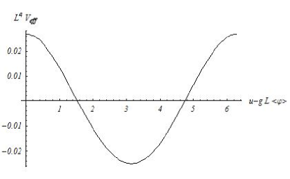
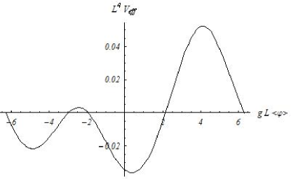
Figure 1: The effective potential for the $U(1)$ model. Left: single fermion species with $\bar{\mu}L=0.01$. Right: two fermion species with $\bar{\mu}_{1}L=0.01,~{}\bar{\mu}_{2}L=0.008$, $u_{1}=2.3,~{}u_{2}=0$ and charges $1$ and $-1/2$; note that for $u_{1}$ the tree-level mass is $\simeq 2.3/L$.

VII ${SU(2)}$ example

We look for an ${SU(2)}$ theory where the light sector is invariant under a $U(1)$ subgroup and contains one complex scalar. We include 2 fermion doublets.

All the constraints are satisfied by the choices

$$\begin{array}[]{ll}{\mathbbm{V}}={\mathbbm{1}}_{3},&\tilde{\mathbbm{V}}={\rm diag}\left(-1,+1,-1\right),\cr&\cr{\cal B}={\rm diag}\left({\mathbbm{1}}_{4},-{\mathbbm{1}}_{4}\right),&{\cal A}={\rm diag}\left({\mathbbm{1}}_{2},-{\mathbbm{1}}_{2},{\mathbbm{1}}_{2},-{\mathbbm{1}}_{2}\right),\cr&\cr{\cal M}=\pmatrix{0&{\bm{\mu}}\cr{\bm{\mu}}&0},&{\bm{\mu}}=\frac{i}{2}\pmatrix{\bar{\mu}_{+}\sigma_{1}&0\cr 0,&\bar{\mu}_{-}\sigma_{1}}\end{array}$$ (30)

(31)

(32)

$$\tau_{1}=\frac{i}{2}\pmatrix{0&-\rho\cr\rho&0},~{}~{}\tau_{2}=\frac{1}{2}\pmatrix{\rho&0\cr 0&-\rho},~{}~{}\tau_{3}=\frac{1}{2}\pmatrix{0&{\mathbbm{1}}_{4}\cr{\mathbbm{1}}_{4}&0},$$ (33)

where $\rho={\rm diag}\left(-1,+1,-1,+1\right)$ and $\bar{\mu}_{\pm}$ are real.

Using (19) these expressions show that the light (tree-level spectrum) consists of a $U(1)$ gauge boson, one Dirac fermion of mass $\bar{\mu}_{+}$ and one charged scalar. The one-loop effective potential has a form similar to (24) and is plotted in fig. 2. This plot seems to indicate that the $U(1)$ symmetry is broken and that there are in fact no massless vector bosons. This is not the case: the masses of the vector Fourier modes are $m_{n}=2\pi n/L+2g\left\langle\phi\right\rangle$; at tree level $\left\langle\phi\right\rangle=0$ so $m_{n}^{\left(\rm tree\right)}=2\pi n/L$ and we identify the $U(1)$ gauge boson with the $n=0$ mode. At one loop $\left\langle\phi\right\rangle=\pm\pi/(Lg)$ so that $m_{n}^{\left(1\rm loop\right)}=2\pi(n\pm 1)/L$ and we identify the $U(1)$ gauge boson with the $n=\mp 1$ mode.

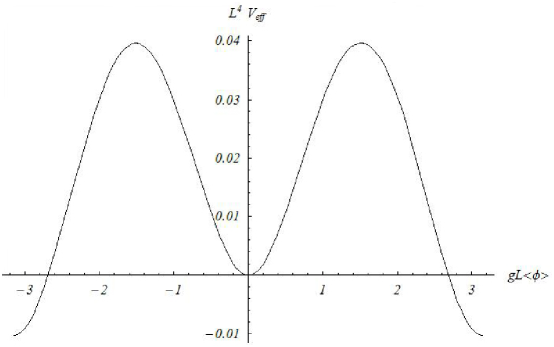
Figure 2: The effective potential for the ${SU(2)}$ model; $\bar{\mu}_{-}L=2.0,~{}\bar{\mu}_{+}L=0.001$.

These results suggest that with the proposed transformation properties (11, 13) these theories could generate the correct low-energy physics. The difficulty lies in constructing an effective potential that has the right value of $\left\langle\phi\right\rangle$. This apparently necessitates the introduction of additional fermion representations which, however, need not be light and would not spoil the light spectrum. These models are currently under investigation.

References

- (1) N. Arkani-Hamed, S. Dimopoulos and G. R. Dvali, Phys. Lett. B 429 (1998) 263 [arXiv:hep-ph/9803315]. I. Antoniadis, N. Arkani-Hamed, S. Dimopoulos and G. R. Dvali, Phys. Lett. B 436 (1998) 257 [arXiv:hep-ph/9804398].
- (2) L. Randall and R. Sundrum, Phys. Rev. Lett. 83 (1999) 3370 [arXiv:hep-ph/9905221]; Phys. Rev. Lett. 83 (1999) 4690 [arXiv:hep-th/9906064].
- (3) T. Appelquist, H. C. Cheng and B. A. Dobrescu, Phys. Rev. D 64 (2001) 035002 [arXiv:hep-ph/0012100].
- (4) H. Hatanaka, Prog. Theor. Phys. 102 (1999) 407 [arXiv:hep-th/9905100]. B. Grzadkowski and J. Wudka, Phys. Rev. Lett. 93, 211603 (2004) [arXiv:hep-ph/0401232].
- (5) For a review see, for example, M. Quiros, arXiv:hep-ph/0302189.
- (6) Y. Hosotani, Annals Phys. 190, 233 (1989); Phys. Lett. B 129 (1983) 193.
- (7) B. Grzadkowski and J. Wudka, arXiv:hep-ph/0501238.