WORKING GROUP I: Parton Distributions
Summary Report for the HERA - LHC Workshop proceedings

Abstract

We provide an assessment of the impact of parton distributions on the determination of LHC processes, and of the accuracy with which parton distributions (PDFs) can be extracted from data, in particular from current and forthcoming HERA experiments. We give an overview of reference LHC processes and their associated PDF uncertainties, and study in detail $W$ and $Z$ production at the LHC. We discuss the precision which may be obtained from the analysis of existing HERA data, tests of consistency of HERA data from different experiments, and the combination of these data. We determine further improvements on PDFs which may be obtained from future HERA data (including measurements of $F_{L}$), and from combining present and future HERA data with present and future hadron collider data. We review the current status of knowledge of higher (NNLO) QCD corrections to perturbative evolution and deep-inelastic scattering, and provide reference results for their impact on parton evolution, and we briefly examine non-perturbative models for parton distributions. We discuss the state-of-the art in global parton fits, we assess the impact on them of various kinds of data and of theoretical corrections, by providing benchmarks of Alekhin and MRST parton distributions and a CTEQ analysis of parton fit stability, and we briefly presents proposals for alternative approaches to parton fitting. We summarize the status of large and small $x$ resummation, by providing estimates of the impact of large $x$ resummation on parton fits, and a comparison of different approaches to small $x$ resummation, for which we also discuss numerical techniques.

1 Introduction

The physics of parton distributions, especially within the context of deep-inelastic scattering (DIS), has been an active subject of detailed theoretical and experimental investigations since the origins of perturbative quantum chromodynamics (QCD), which, thanks to asymptotic freedom, allows one to determine perturbatively their scale dependence [1, 2, 3, 4, 5].

Since the advent of HERA, much progress has been made in determining the Parton Distribution Functions (PDFs) of the proton. A good knowledge of the PDFs is vital in order to make predictions for both Standard Model and beyond the Standard Model processes at hadronic colliders, specifically the LHC. Furthermore, PDFs must be known as precisely as possible in order to maximize the discovery potential for new physics at the LHC. Conversely, LHC data will lead to an imporvement in the knowledge of PDFs.

The main aim of this document is to provide a state-of-the art assessment of the impact of parton distributions on the determination of LHC processes, and of the accuracy with which parton distributions can be extracted from data, in particular current and forthcoming HERA data.

In Section 2 we will set the stage by providing an overview of relevant LHC processes and a discussion of their experimental and theoretical accuracy. In Section 3 we will turn to the experimental determination of PDFs, and in particular examine the improvements to be expected from forthcoming measurements at HERA, as well as from analysis methods which allow one to combine HERA data with each other, and also with data from existing (Tevatron) and forthcoming (LHC) hadron colliders. In Section 4 we will discuss the state of the art in the extraction of parton distributions of the data, by first reviewing recent progress in higher-order QCD corrections and their impact on the extraction of PDFs, and then discussing and comparing the determination of PDFs from global fits. Finally, in Section 5 we will summarize the current status of resummed QCD computations which are not yet used in parton fits, but could lead to an improvement in the theoretical precision of PDF determinations.

Whereas we will aim at summarizing the state of the art, we will also provide several new results, benchmarks and predictions, which have been obtained within the framework of the HERA-LHC workshop.

2 LHC final states and their potential experimental and theoretical accuracies

2.1 Introduction

Cross section calculations and experimental simulations for many LHC reactions, within the Standard Model and for many new physics scenarios have been performed during the last 20 years. These studies demonstrate how various final states might eventually be selected above Standard Model backgrounds and indicate the potential statistical significance of such measurements. In general, these studies assumed that the uncertainties from various sources, like the PDF uncertainties, the experimental uncertainties and the various signal and background Monte Carlo simulations will eventually be controlled with uncertainties small compared to the expected statistical significance. This is the obvious approach for many so called discovery channels with clean and easy signatures and relatively small cross sections.

However, during the last years many new and more complicated signatures, which require more sophisticated selection criteria, have been discussed. These studies indicate the possibility to perform more ambitious searches for new physics and for precise Standard Model tests, which would increase the physics potential of the LHC experiments. Most of these studies concentrate on the statistical significance only and potential systematic limitations are rarely discussed.

In order to close this gap from previous LHC studies, questions related to the systematic limits of cross section measurements from PDF uncertainties, from imperfect Standard Model Monte Carlo simulations, from various QCD uncertainties and from the efficiency and luminosity uncertainties were discussed within the PDF working group of this first HERA-LHC workshop. The goal of the studies presented during the subgroup meetings during the 2004/5 HERA LHC workshop provide some answers to questions related to these systematic limitations. In particular, we have discussed potential experimental and theoretical uncertainties for various Standard Model signal cross sections at the LHC. Some results on the experimental systematics, on experimental and theoretical uncertainties for the inclusive W, Z and for diboson production, especially related to uncertainties from PDF’s and from higher order QCD calculations are described in the following sections.

While it was not possible to investigate the consequences for various aspects of the LHC physics potential in detail, it is important to keep in mind that many of these Standard Model reactions are also important backgrounds in the search for the Higgs and other exotic phenomena. Obviously, the consequences from these unavoidable systematic uncertainties need to be investigated in more detail during the coming years.

2.2 Measuring and interpreting cross sections at the LHC

The LHC is often called a machine to make discoveries. However, after many years of detailed LHC simulations, it seems clear that relatively few signatures exist, which do not involve cross section measurements for signals and the various backgrounds. Thus, one expects that cross section measurements for a large variety of well defined reactions and their interpretation within or perhaps beyond the Standard Model will be one of the main task of the LHC physics program.

While it is relatively easy to estimate the statistical precision of a particular measurement as a function of the luminosity, estimates of potential systematic errors are much more complicated. Furthmore, as almost nobody wants to know about systematic limitations of future experiments, detailed studies are not rewarding. Nevertheless, realistic estimates of such systematic errors are relevant, as they might allow the LHC community to concentrate their efforts on the areas where current systematic errors, like the ones which are related to uncertainties from Parton Distribution Functions (PDF) or the ones from missing higher order QCD calculations, can still be improved during the next years.

In order to address the question of systematics, it is useful to start with the basics of cross section measurements. Using some clever criteria a particular signature is separated from the data sample and the surviving N_observed events can be counted. Backgrounds, N_background, from various sources have to be estimated either using the data or some Monte Carlo estimates. The number of signal events, N_signal, is then obtained from the difference. In order to turn this experimental number of signal events into a measurement one has to apply a correction for the efficiency. This experimental number can now be compared with the product of the theoretical production cross section for the considered process and the corresponding Luminosity. For a measurement at a hadron collider, like the LHC, processes are calculated on the basis of quark and gluon luminosities which are obtained from the proton-proton luminosity “folded” with the PDF’s.

In order to estimate potential systematic errors one needs to examine carefully the various ingredients to the cross section measurement and their interpretation. First, a measurement can only be as good as the impact from of the background uncertainties, which depend on the optimized signal to background ratio. Next, the experimental efficiency uncertainty depends on many subdetectors and their actual real time performance. While this can only be known exactly from real data, one can use the systematic error estimates from previous experiments in order to guess the size of similar error sources for the future LHC experiments. We are furthermore confronted with uncertainties from the PDF’s and from the proton-proton luminosity. If one considers all these areas as essentially experimental, then one should assign uncertainties originating from imperfect knowledge of signal and background cross sections as theoretical.

Before we try to estimate the various systematic errors in the following subsections, we believe that it is important to keep in mind that particular studies need not to be much more detailed than the largest and limiting uncertainty, coming from either the experimental or the theoretical area. Thus, one should not waste too much time, in order to achieve the smalled possible uncertainty in one particular area. Instead, one should try first to reduce the most important error sources and if one accepts the “work division” between experimental and theoretical contributions, then one should simply try to be just a little more accurate than either the theoretical or the experimental colleagues.

2.2.1 Guessing experimental systematics for ATLAS and CMS

In order to guess experimental uncertainties, without doing lengthy and detailed Monte Carlo studies, it seems useful to start with some simple and optimistic assumptions about ATLAS and CMS.

First of all, one should assume that both experiments can actually operate as planned in their proposals. As the expected performance goals are rather similar for both detectors the following list of measurement capabilities looks as a reasonable first guess.

• Isolated electrons, muons and photons with a transverse momentum above 20 GeV and a pseudorapidity $\eta$ with $|\eta|\leq 2.5$ are measured with excellent accuracy and high (perhaps as large as 95% for some reactions) “homogeneous” efficiency. Within the pseudo rapidity coverage one can assume that experimentalists will perhaps be able, using the large statistics from leptonic W and Z decays, to control the efficiency for electrons and muons with a 1% accuracy. For simplicity, one can also assume that these events will allow to control measurements with high energy photons to a similar accuracy. For theoretical studies one might thus assume that high $p_{t}$ electrons, muons and photons and $|\eta|\leq 2.5$ are measured with a systematic uncertainty of $\pm$ 1% for each lepton (photon).

• Jets are much more difficult to measure. Optimistically one could assume that jets can be seen with good efficiency and angular accuracy if the jet transverse momentum is larger than 30 GeV and if their pseudo rapidity fulfills $|\eta|\leq 4.5$. The jet energy resolution is not easy to quantify, but numbers could be given using some “reasonable” assumptions like $\Delta E/E\approx 100-150\%/\sqrt{E}$. For various measurements one want to know the uncertainty of the absolute jet energy scale. Various tools, like the decays of $W\rightarrow q\bar{q}$ in $t\bar{t}$ events or the photon-jet final state, might be used to calibrate either the mean value or the maximum to reasonably good accuracy. We believe that only detailed studies of the particular signature will allow a quantitative estimate of the uncertainties related to the jet energy scale measurements.

• The tagging of b–flavoured jets can be done, but the efficiency depends strongly on the potential backgrounds. Systematic efficiency uncertainties for the b–tagging are difficult to quantify but it seems that, in the absence of a new method, relative b-tagging uncertainties below $\pm$ 5% are almost impossible to achieve.

With this baseline LHC detector capabilities, it seems useful to divide the various high $q^{2}$ LHC reactions into essentially five different non overlapping categories. Such a devision can be used to make some reasonable accurate estimates of the different systematics.

• Drell–Yan type lepton pair final states. This includes on– and off–shell W and Z decays.

• $\gamma$–jet and $\gamma\gamma X$ final states.

• Diboson events of the type $WW,~{}WZ,~{}ZZ,~{}W\gamma$ with leptonic decays of the $W$ and $Z$ bosons. One might consider to include the Standard Model Higgs signatures into this group of signatures.

• Events with top quarks in the final state, identified with at least one isolated lepton.

• Hadronic final states with up to n(=2,3 ..) Jets and different $p_{t}$ and mass.

With this “grouping” of experimental final states, one can now start to analyze the different potential error sources. Where possible, one can try to define and use relative measurements of various reactions such that some systematic errors will simply cancel.

Starting with the resonant W and Z production with leptonic decays, several million of clean events will be collected quickly, resulting in relative statistical errors well below $\pm$1%. Theoretical calculations for these reactions are well advanced and these reactions are among the best understood LHC final states allowing to build the most accurate LHC Monte Carlo generators. Furthermore, some of the experimental uncertainties can be reduced considerably if ratio measurements of cross section, such as $W^{+}/W^{-}$ and $Z/W$, are performed. The similarities in the production mechanism should also allow to reduce theoretical uncertainties for such ratios. The experimental counting accuracy of W and Z events, which includes background and efficiency corrections, might achieve eventually uncertainties of 1% or slightly better for cross section ratios.

Furthermore, it seems that the shape of the $p_{t}$ distribution of the Z, using the decay into electron pairs ($pp\rightarrow ZX\rightarrow e{+}e^{-}X$), can be determined with relative accuracies of much less than 1%. This distribution, shown in figure 1, can be used to tune the Monte Carlo description of this particular process. This tuning of the Monte Carlo can than be used almost directly to predict theoretically also the W $p_{t}$ spectrum, and the $p_{t}$ spectrum for high mass Drell-Yan lepton pair events. Once an accurate model description of these Standard Model reactions is achieved one might use these insights also to predict the $p_{t}$ spectrum of other well defined final states.

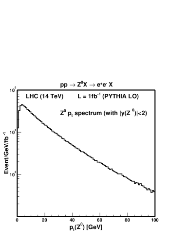
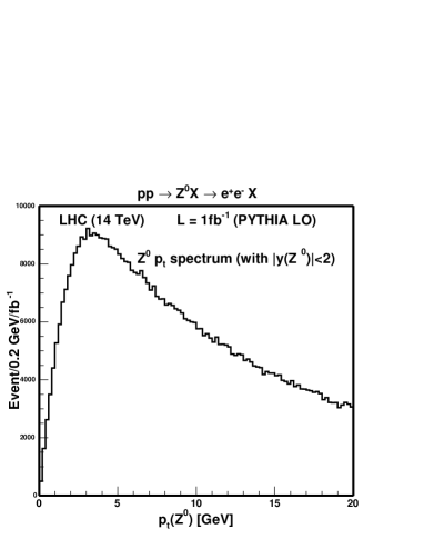
Figure 1: Simple simulation of a potential measurement of the Z $p_{t}$ spectrum, possible with a luminosity of only 1 fb^-1. Who will be able to predict this $p_{t}$ spectrum in all its beauty and with similar accuracy?

From all the various high $q^{2}$ reactions, the inclusive production of W and Z events is known to be the theoretically best understood and best experimentally measurable LHC reaction. Consequently, the idea to use these simple well defined final states as the LHC cross section normalisation tool, or standard candle was described first in reference [6]. This study indicated that the W and Z production might result in a precise and simple parton luminosity monitor. In addition, these reactions can also be used to improve the relative knowledge of the PDF’s. In fact, if one gives up on the idea to measure absolute cross sections, the relative parton luminosity can in principle be determined with relative uncertainties well below $\pm$5%, the previously expected possible limit for any absolut proton-proton luminosity normalisation procdure.

In summary, one can estimate that it should be possible to reduce experimental uncertainties for Drell-Yan processes to systematic uncertainties below $\pm$5%, optimistically one might envisage an event counting accuracy of perhaps $\pm$1%, limited mainly from the lepton identification efficiency.

The next class of final states, which can be measured exclusively with leptons, are the diboson pair events with subsequent leptonic decays. Starting with the ZZ final state, we expect that the statistical accuracy will dominate the measurement for several years. Nevertheless, the systematic uncertainties of the measurement, based on four leptons, should in principle be possible with relative errors of a few % only.

The production of WZ and WW involves unmeasurable neutrinos. Thus, experimentally only an indirect and incomplete determination of the kinematics of the final states is possible and very detailed simulations with precise Monte Carlo generators are required for the interpretation of these final state. It seems that a measurement of the event counting with an accuracy below $\pm$5%, due to efficiency uncertainties from the selection alone, to be highly non trivial. Nevertheless, if the measurements and the interpretations can be done relative to the W and Z resonance production, some uncertainties from the lepton identification efficiency, from the PDF and from the theoretical calculation can perhaps be reduced. Without going into detailed studies for each channel, one could try to assume that a systematic uncertainty of $\pm$5% might be defined as a goal. Similar characteristics and thus limitations can be expected for other diboson signatures.

The production cross section of top antitop quark pairs is large and several million of semileptonic tagged and relatively clean events ($pp\rightarrow t\bar{t}\rightarrow WbWb$ identified with one leptonic $W$ decay) can be expected. However, the signature involves several jets, some perhaps tagged as b–flavoured, and missing transverse momentum from the neutrino(s). The correct association of the various jets to the corresponding top quark is known to be extremely difficult, leading to large combinatorial backgrounds. Thus, it seems that, even if precise Monte Carlo generators will become eventually available, that systematic uncertainties smaller than 5-10% should not be expected. Consequently,we assume that top antitop backgrounds for a wide class of signals can not be determined with uncertainties smaller than 5-10%.

Measurements of so called “single” top quarks are even more difficult, as the cross section is smaller and larger backgrounds exist. Systematic errors will therefore always be larger than the one guessed for top-antitop pair production.

Finally, we can address the QCD jet production. Traditionally one measures and interprets the so called jet cross section as a function of $p_{t}$ jet and the mass of the multi jet system using various rapidity intervals. With the steeply falling $p_{t}$ jet spectrum and essentially no background, one will determine the differential spectrum such that only the slope has to be measured with good relative accuracy. If one is especially interested into the super high mass or high $p_{t}$ events, then we expect that migrations due to jet mis-measurements and non Gaussian tails in the jet energy measurements will limit any measurement. A good guess might be that the LHC experiments can expect absolut normalisation uncertainties similar to the ones achieved with CDF and D0, corresponding to uncertainties of about $\pm$ 10-20%.

Are the above estimated systematic limits for the various measurements pessimistic, optimistic or simply realistic? Of course, only real experiments will tell during the coming LHC years. However, while some of these estimates will need perhaps some small modification, they could be used as a limit waiting to be improved during the coming years. Thus, some people full of ideas might take these numbers as a challenge, and discover and develop new methods that will improve these estimates. This guess of systematic limitations for LHC experiments could thus be considered as a “provocation”, which will stimulate activities to prove them wrong. In fact, if the experimental and theoretical communities could demonstrate why some of these “pessimistic” numbers are wrong the future real LHC measurements will obviously benefit from the required efforts to develope better Monte Carlo programs and better experimental methods.

The following summary from a variety of experimental results from previous high energy collider experiments might help to quantify particular areas of concern for the LHC measurements. These previous measurements can thus be used as a starting point for an LHC experimenter, who can study and explain why the corresponding errors at LHC will be smaller or larger.

2.2.2 Learning from previous collider experiments

It is broadly accepted, due to the huge hadronic interaction rate and the short bunch crossing time, that the experimental conditions at the LHC will be similar or worse than the ones at the Tevatron collider. One experimental answer was to improve the granularity, speed and accuracy of the different detector elements accordingly. Still, no matter how well an experiment can be realized, the LHC conditions to do experiments will be much more difficult than at LEP or any hypothetical future high energy $e^{+}e^{-}$ collider. One important reason is the large theoretical uncertainty, which prevents to make signal and background Monte Carlos with accuracies similar to the ones which were used at LEP.

Thus, we can safely expect that systematic errors at LHC experiments will be larger than the corresponding ones from LEP and that the Tevatron experience can be used as a first guess.

• Measurement of $\sigma\times$BR for W and Z production from CDF[7] and D0[8]:

  The CDF collaboration has presented a high statistics measurement with electrons and muons. Similar systematic errors of about $\pm$ 2% were achieved for efficiency and thus the event counting with electrons and muons. The error was reduced to $\pm$ 1.4% for the ratio measurement where some lepton identification efficiencies cancel. Similar errors about $\times$ 1.5-2 larger have been obtained by the corresponding measurements from the D0 experiment.

• Measurement of the cross section for $p\bar{p}\rightarrow Z\gamma(\gamma)$ from D0[9]:

  A total of 138 $ee\gamma$ and 152 $\mu\mu\gamma$ candidate events were selected. The background was estimated to be about 10% with a systematic uncertainty of $\pm$ 10-15%, mainly from $\gamma$-jet misidentification. Using Monte Carlo and a large sample of inclusive Z events, the efficiency uncertainty has been estimated to be $\approx$ 5% and when the data were used in comparison with the Standard Model prediction another uncertainty of 3.3% originating from PDF’s was added.

• Measurement of the $p\bar{p}\rightarrow t\bar{t}$ production cross section from CDF[10]

  A recent CDF measurement, using 197 pb^-1, obtained a cross section (in pb) of 7.0 +2.4 (-2.1) from statistics. This should be comapred with +1.7 (-1.2) from systematics, which includes $\pm 0.4$ from the luminosity measurement. Thus, uncertainties from efficiency and background are roughly $\pm$20%. It is expected that some of the uncertainties can be reduced with the expected 10 fold luminosity increase such that the systematic error will eventually decrease to about $\pm$ 10%, sufficient to be better than the expected theoretical error of $\pm$ 15%.

• A search for Supersymmetry with b-tagged jets from CDF[11]:

  This study, using single and double b-tagged events was consistent with background only. However, it was claimed that the background uncertainty was dominated by the systematic error, which probably originated mostly from the b tagging efficiency and the misidentification of b-flavoured jets. The numbers given were 16.4$\pm$ 3.7 events (3.15 from systematics) for the single b-tagged events and 2.6$\pm$0.7 events (0.66 from systematics) for the double b-tagged events. These errors originate mainly from the b-tagging efficiency uncertainties, which are found to roughly $\pm$ 20-25% for this study of rare events.

• Some “random” selection of recent $e^{+}e^{-}$ measurements:

  A recent measurement from ALEPH (LEP) of the W branching ratio to $q\bar{q}$ estimated a systematic uncertainty of about $\pm$ 0.2% [12]. This small uncertainty was possible because many additional constraints could be used.

  OPAL has reported a measurement of $R_{b}$ at LEP II energies, with a systematic uncertainty of $\pm$ 3.7%. Even though this uncertainty could in principle be reduced with higher statistics, one can use it as an indication on how large efficiency uncertainties from b-tagging are already with clean experimental conditions[13]

  Recently, ALEPH and DELPHI have presented cross section measurements for $e^{+}e^{-}\rightarrow\gamma\gamma$ with systematic errors between 2.2% (ALEPH)[14] and 1.1% (DELPHI)[15]. In both cases, the efficiency uncertainty, mainly from conversions, for this in principle easy signal was estimated to be roughly 1%. In the case of ALEPH an uncertainty of about $\pm$0.8% was found for the background correction.

Obviously, these measurements can only be used, in absence of anything better, as a most optimistic guess for possible systematic limitations at a hadron collider. One might conclude that the systematics from LEP experiments give (1) an optimistic limit for comparable signatures at the LHC and (2) that the results from CDF and D0 should indicate systematics which might be obtained realistically during the early LHC years.

Thus, in summary the following list might be used as a first order guess on achievable LHC systematics.

• “Isolated” muons, electrons and photons can be measured with a small momentum (energy) uncertainty and with an almost perfect angular resolution. The efficiency for $p_{t}\geq 20$ GeV and $|\eta|\leq 2.5$ will be “high” and can be controlled optimistically to $\pm$ 1%. Some straight forward selection criteria should reduce jet background to small or negligible levels.

• “Isolated” jets with a $p_{t}\geq 30$ GeV and $|\eta|\leq 4.5$ can be seen with high (veto) efficiency and a small uncertainty from the jet direction measurement. However, it will be very difficulty to measure the absolute jet energy scale and Non-Gaussian tails will limit the systematics if the jet energy scale is important.

• Measurements of the missing transverse momentum depend on the final state but will in general be a sum of the errors from the lepton and the jet accuracies.

Using these assumptions, the following “optimistic” experimental systematic errors can be used as a guideline:

1. Efficiency uncertainties for isolated leptons and photons with a $p_{t}$ above 20 GeV can be estimated with a $\pm$1% accuracy.

2. Efficiencies for tagging jets will be accurate to a few percent and the efficiency to tag b-flavoured jets will be known at best within $\pm$5%.

3. Backgrounds will be known, combining theoretical uncertainties and some experimental determinations, at best with a $\pm$5-10% accuracy. Thus, discovery signatures without narrow peaks require signal to background ratios larger than 0.25-0.5, if 5 $\sigma$ discoveries are claimed. Obviously, for accurate cross section measurements, the signal to background ratio should be much larger.

4. In case of ratio measurements with isolated leptons, like $pp\rightarrow W^{+}/pp\rightarrow W^{-}$, relative errors between 0.5-1% should be possible. Furthermore, it seems that the measurement of the shape of Z $p_{t}$ spectrum, using Z$\rightarrow e^{+}e^{-}$, will be possible with a systematic error much smaller than 1%. As the Z cross section is huge and clean we expect that this signature will become the best measurable final state and should allow to test a variety of production models with errors below $\pm$ 1%, thus challenging future QCD calculations for a long time.

2.3 Uncertainties on $W$ and $Z$ production at the LHC

2.3.1 Introduction

At leading order (LO), $W$ and $Z$ production occur by the process, $q\bar{q}\rightarrow W/Z$, and the momentum fractions of the partons participating in this subprocess are given by $x_{1,2}=\frac{M}{\surd{s}}\exp(\pm y)$, where $M$ is the centre of mass energy of the subprocess, $M=M_{W}$ or $M_{Z}$, $\surd{s}$ is the centre of mass energy of the reaction ($\surd{s}=14$ TeV at the LHC) and $y=\frac{1}{2}\ln{\frac{(E+p_{l})}{(E-p_{l})}}$ gives the parton rapidity. The kinematic plane for LHC parton kinematics is shown in Fig. 2. Thus, at central rapidity, the participating partons have small momentum fractions, $x\sim 0.005$. Moving away from central rapidity sends one parton to lower $x$ and one to higher $x$, but over the measurable rapidity range, $|y|<2.5$, $x$ values remain in the range, $10^{-4}<x<0.1$. Thus, in contrast to the situation at the Tevatron, valence quarks are not involved, the scattering is happening between sea quarks. Furthermore, the high scale of the process $Q^{2}=M^{2}\sim 10,000$ GeV² ensures that the gluon is the dominant parton, see Fig. 2, so that these sea quarks have mostly been generated by the flavour blind $g\to q\bar{q}$ splitting process. Thus the precision of our knowledge of $W$ and $Z$ cross-sections at the LHC is crucially dependent on the uncertainty on the momentum distribution of the gluon.

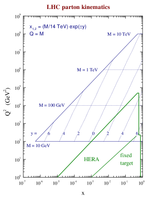
Figure 2: Left plot: The LHC kinematic plane (thanks to James Stirling). Right plot: PDF distributions at $Q^{2}=10,000$ GeV².

HERA data have dramatically improved our knowledge of the gluon, as illustrated in Fig. 3, which shows $W$ and $Z$ rapidity spectra predicted from a global PDF fit which does not include the HERA data, compared to a fit including HERA data. The latter fit is the ZEUS-S global fit [16], whereas the former is a fit using the same fitting analysis but leaving out the ZEUS data. The full PDF uncertainties for both fits are calculated from the error PDF sets of the ZEUS-S analysis using LHAPDF [17] (see the contribution of M.Whalley to these proceedings). The predictions for the $W/Z$ cross-sections, decaying to the lepton decay mode, are summarised in Table 1.

PDF Set $\sigma(W^{+}).B(W^{+}\rightarrow l^{+}\nu_{l})$ $\sigma(W^{-}).B(W^{-}\rightarrow l^{-}\bar{\nu}_{l})$ $\sigma(Z).B(Z\rightarrow l^{+}l^{-})$ ZEUS-S no HERA $10.63\pm 1.73$ nb $7.80\pm 1.18$ nb $1.69\pm 0.23$ nb ZEUS-S $12.07\pm 0.41$ nb $8.76\pm 0.30$ nb $1.89\pm 0.06$ nb CTEQ6.1 $11.66\pm 0.56$ nb $8.58\pm 0.43$ nb $1.92\pm 0.08$ nb MRST01 $11.72\pm 0.23$ nb $8.72\pm 0.16$ nb $1.96\pm 0.03$ nb

Table 1: LHC $W/Z$ cross-sections for decay via the lepton mode, for various PDFs

The uncertainties in the predictions for these cross-sections have decreased from $\sim 16\%$ pre-HERA to $\sim 3.5\%$ post-HERA. The reason for this can be seen clearly in Fig. 4, where the sea and gluon distributions for the pre- and post-HERA fits are shown for several different $Q^{2}$ bins, together with their uncertainty bands. It is the dramatically increased precision in the low-$x$ gluon PDF, feeding into increased precision in the low-$x$ sea quarks, which has led to the increased precision on the predictions for $W/Z$ production at the LHC.

Figure 3: LHC $W^{+},W^{-},Z$ rapidity distributions and their PDF uncertainties (the full line shows the central value and the dashed lines show the spread of the uncertainty): Top Row: from the ZEUS-S global PDF analysis not including HERA data; left plot $W^{+}$; middle plot $W^{-}$; right plot $Z$: Bottom Row: from the ZEUS-S global PDF analysis including HERA data; left plot $W^{+}$; middle plot $W^{-}$; right plot $Z$

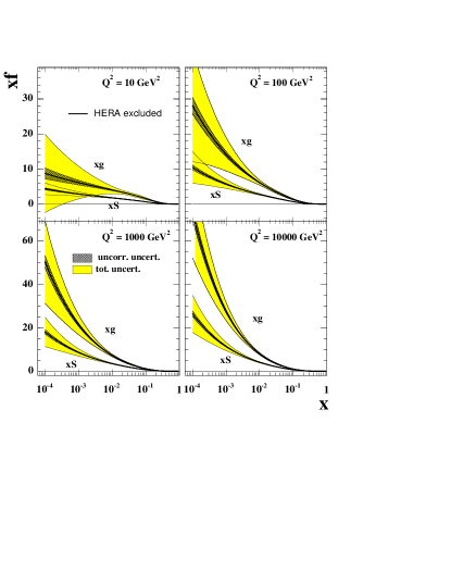
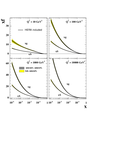
Figure 4: Sea ($xS$) and gluon ($xg$) PDFs at various $Q^{2}$: left plot; from the ZEUS-S global PDF analysis not including HERA data; right plot: from the ZEUS-S global PDF analysis including HERA data. The inner cross-hatched error bands show the statistical and uncorrelated systematic uncertainty, the outer error bands show the total uncertainty including experimental correlated systematic uncertainties, normalisations and model uncertainty.

Further evidence for the conclusion that the uncertainties on the gluon PDF at the input scale ($Q^{2}_{0}=7$ GeV², for ZEUS-S) are the major contributors to the uncertainty on the $W/Z$ cross-sections at $Q^{2}=M_{W}(M_{Z})$, comes from decomposing the predictions down into their contributing eigenvectors. Fig 5 shows the dominant contributions to the total uncertainty from eigenvectors 3, 7, and 11 which are eigenvectors which are dominated by the parameters which control the low-$x$, mid-$x$ and high-$x$, gluon respectively.

Figure 5: LHC $W^{+}$ rapidity distributions and their PDF uncertainties due to the eigenvectors 3,7 and 11 of the ZEUS-S analysis.

The post-HERA level of precision illustrated in Fig. 3 is taken for granted in modern analyses, such that $W/Z$ production have been suggested as ‘standard-candle’ processes for luminosity measurement. However, when considering the PDF uncertainties on the Standard Model (SM) predictions it is necessary not only to consider the uncertainties of a particular PDF analysis, but also to compare PDF analyses. Fig. 6 compares the predictions for $W^{+}$ production for the ZEUS-S PDFs with those of the CTEQ6.1[18] PDFs and the MRST01[19] PDFs. The corresponding $W^{+}$ cross-sections, for decay to leptonic mode are given in Table 1. Comparing the uncertainty at central rapidity, rather than the total cross-section, we see that the uncertainty estimates are rather larger: $~{}5.2\%$ for ZEUS-S; $~{}8.7\%$ for CTEQ6.1M and about $~{}3.6\%$ for MRST01. The difference in the central value between ZEUS-S and CTEQ6.1 is $~{}3.5\%$. Thus the spread in the predictions of the different PDF sets is comparable to the uncertainty estimated by the individual analyses. Taking all of these analyses together the uncertainty at central rapidity is about $~{}8\%$.

Figure 6: LHC $W^{+}$ rapidity distributions and their PDF uncertainties: left plot, ZEUS-S PDFs; middle plot, CTEQ6.1 PDFs; right plot: MRST01 PDFs.

Since the PDF uncertainty feeding into the $W^{+},W^{-}$ and $Z$ production is mostly coming from the gluon PDF, for all three processes, there is a strong correlation in their uncertainties, which can be removed by taking ratios. Fig. 7 shows the $W$ asymmetry

$$A_{W}=(W^{+}-W^{-})/(W^{+}+W^{-}).$$

for CTEQ6.1 PDFs, which have the largest uncertainties of published PDF sets. The PDF uncertainties on the asymmetry are very small in the measurable rapidity range. An eigenvector decomposition indicates that sensitivity to high-$x$ $u$ and $d$ quark flavour distributions is now evident at large $y$. Even this residual flavour sensitivity can be removed by taking the ratio

$$A_{ZW}=Z/(W^{+}+W^{-})$$

as also shown in Fig. 7. This quantity is almost independent of PDF uncertainties. These quantities have been suggested as benchmarks for our understanding of Standard Model Physics at the LHC. However, whereas the $Z$ rapidity distribution can be fully reconstructed from its decay leptons, this is not possible for the $W$ rapidity distribution, because the leptonic decay channels which we use to identify the $W$’s have missing neutrinos. Thus we actually measure the $W$’s decay lepton rapidity spectra rather than the $W$ rapidity spectra. The lower half of Fig. 7 shows the rapidity spectra for positive and negative leptons from $W^{+}$ and $W^{-}$ decay and the lepton asymmetry,

$$A_{l}=(l^{+}-l^{-})/(l^{+}+l^{-}).$$

A cut of, $p_{tl}>25$ GeV, has been applied on the decay lepton, since it will not be possible to trigger on leptons with small $p_{tl}$. A particular lepton rapidity can be fed from a range of $W$ rapidities so that the contributions of partons at different $x$ values is smeared out in the lepton spectra, but the broad features of the $W$ spectra and the sensitivity to the gluon parameters remain. The lepton asymmetry shows the change of sign at large $y$ which is characteristic of the $V-A$ structure of the lepton decay. The cancellation of the uncertainties due to the gluon PDF is not so perfect in the lepton asymmetry as in the $W$ asymmetry. Nevertheless in the measurable rapidity range sensitivity to PDF parameters is small. Correspondingly, the PDF uncertainties are also small ($~{}4\%$) and this quantity provides a suitable Standard Model benchmark.

Figure 7: Predictions for $W,Z$ production at the LHC from the CTEQ6.1 PDFs. Top row: left plot, the $W$ asymmetry, $A_{W}$; right plot, the ratio, $A_{ZW}$: Bottom row: left plot, decay $e^{+}$ rapidity spectrum; middle plot, decay $e^{-}$ rapidity spectrum; right plot, lepton asymmetry, $A_{e}$

In summary, these preliminary investigations indicate that PDF uncertainties on predictions for the $W,Z$ rapidity spectra, using standard PDF sets which describe all modern data, have reached a precision of $\sim 8\%$. This may be good enough to consider using these processes as luminosity monitors. The predicted precision on ratios such as the lepton ratio, $A_{l}$, is better ($\sim 4\%$) and this measurement may be used as a SM benchmark. It is likely that this current level of uncertainty will have improved before the LHC turns on- see the contribution of C. Gwenlan (section 3.2) to these proceedings. The remainder of this contribution will be concerned with the question: how accurately can we measure these quantities and can we use the early LHC data to improve on the current level of uncertainty?

2.3.2 k-factor and PDF re-weighting

To investigate how well we can really measure $W$ production we need to generate samples of Monte-Carlo (MC) data and pass them through a simulation of a detector. Various technical problems arise. Firstly, many physics studies are done with HERWIG (6.505)[20], which generates events at LO with parton showers to account for higher order effects. Distributions can be corrected from LO to NLO by k-factors which are applied as a function of the variable of interest. The use of HERWIG is gradually being superceded by MC@NLO (2.3)[21] but this is not yet implemented for all physics processes. Thus it is necessary to investigate how much bias is introduced by using HERWIG with k-factors. Secondly, to simulate the spread of current PDF uncertainties, it is necessary to run the MC with all of the eigenvector error sets of the PDF of interest. This would be unreasonably time-consuming. Thus the technique of PDF reweighting has been investigated.

One million $W\to e\nu_{e}$ events were generated using HERWIG (6.505). This corresponds to 43 hours of LHC running at low luminosity, $10fb^{-1}$. The events are split into $W^{+}$ and $W^{-}$ events according to their Standard Model cross-section rates, $58\%$: $42\%$ (the exact split depends on the input PDFs). These events are then weighted with k-factors, which are analytically calculated as the ratio of the NLO to LO cross-section as a function of rapidity for the same input PDF [22]. The resultant rapidity spectra for $W^{+},W^{-}$ are compared to rapidity spectra for $\sim 107,700$ events generated using MC@NLO(2.3) in Fig 8. The MRST02 PDFs were used for this investigation. The accuracy of this study is limited by the statistics of the MC@NLO generation. Nevertheless it is clear that HERWIG with k-factors does a good job of mimicking the NLO rapidity spectra. However, the normalisation is too high by $3.5\%$. This is not suprising since, unlike the analytic code, HERWIG is not a purely LO calculation, parton showering is also included. This normalisation difference is not too crucial since in an analysis on real data the MC will only be used to correct data from the detector level to the generator level. For this purpose, it is essential to model the shape of spectra to understand the effect of experimental cuts and smearing but not essential to model the overall normalisation perfectly. However, one should note that HERWIG with k-factors is not so successful in modelling the shape of the $p_{t}$ spectra, as shown in the right hand plot of Fig. 8. This is hardly surprising, since at LO the $W$ have no $p_{t}$ and non-zero $p_{t}$ for HERWIG is generated by parton showering, whereas for MC@NLO non-zero $p_{t}$ originates from additional higher order processes which cannot be scaled from LO, where they are not present.

Figure 8: Top Row: $W$ rapidity and $p_{t}$ spectra for events generated with HERWIG + k-Factors (full line), compared to those generated by MC@NLO (dashed line); left plot $W^{+}$ rapidity; middle plot $W^{-}$ rapidity; right plot $W^{-}$ $p_{t}$. Bottom row: the fractional differences of the spectra generated by HERWIG + k-factors and those generated by MC@NLO. The full line represents the weighted mean of these difference spectra and the dashed lines show its uncertainty

Suppose we generate $W$ events with a particular PDF set: PDF set 1. Any one event has the hard scale, $Q^{2}=M_{W}^{2}$, and two primary partons of flavours $flav_{1}$ and $flav_{2}$, with momentum fractions $x_{1},x_{2}$ according to the distributions of PDF set 1. These momentum fractions are applicable to the hard process before the parton showers are implemented in backward evolution in the MC. One can then evaluate the probability of picking up the same flavoured partons with the same momentum fractions from an alternative PDF set, PDF set 2, at the same hard scale. Then the event weight is given by

$$\rm{PDF(re-weight)}=\frac{f_{PDF_{2}}(x_{1},flav_{1},Q^{2}).f_{PDF_{2}}(x_{2},flav_{2},Q^{2})}{f_{PDF_{1}}(x_{1},flav_{1},Q^{2}).f_{PDF_{1}}(x_{2},flav_{2},Q^{2})}$$ (1)

where $xf_{PDF}(x,flav,Q^{2})$ is the parton momentum distribution for flavour, $flav$, at scale, $Q^{2}$, and momentum fraction, $x$. Fig. 9 compares the $W^{+}$ and $W^{-}$ spectra for a million events generated using MRST02 as PDF set 1 and re-weighting to CTEQ6.1 as PDF set 2, with a million events which are directly generated with CTEQ6.1. Beneath the spectra the fractional difference between these distributions is shown. These difference spectra show that the reweighting is good to better than $1\%$, and there is no evidence of a $y$ dependent bias. This has been checked for reweighting between MRST02, CTEQ6.1 and ZEUS-S PDFs. Since the uncertainties of any one analysis are similar in size to the differences between the analyses it is clear that the technique can be used to produce spectra for the eigenvector error PDF sets of each analysis and thus to simulate the full PDF uncertainties from a single set of MC generated events. Fig. 9 also shows a similar comparison for $p_{t}$ spectra.

Figure 9: Left side: $W^{-}$ (left) and $W^{+}$ (right) rapidity spectra, for events generated with MRST02 PDFs reweighted to CTEQ6.1 PDFs (full line), compared to events generated directly with CTEQ6.1 PDFs (dashed line). The fractional difference between these spectra are also shown beneath the plots. The full line represents the weighted mean of these difference spectra and the dashed lines show its uncertainty. Right side: the same for $p_{t}$ spectra.

2.3.3 Background Studies

To investigate the accuracy with which $W$ events can be measured at the LHC it is necessary to make an estimate of the importance of background processes. We focus on $W$ events which are identified through their decay to the $W\rightarrow e~{}\nu_{e}$ channel. There are several processes which can be misidentified as $W\rightarrow e\nu_{e}$. These are: $W\rightarrow\tau\nu_{\tau}$, with $\tau$ decaying to the electron channel; $Z\rightarrow\tau^{+}\tau^{-}$ with at least one $\tau$ decaying to the electron channel (including the case when both $\tau$’s decay to the electron channel, but one electron is not identified); $Z\rightarrow e^{+}e^{-}$ with one electron not identified. We have generated one million events for each of these background processes, using HERWIG and CTEQ5L, and compared them to one million signal events generated with CTEQ6.1. We apply event selection criteria designed to eliminate the background preferentially. These criteria are:

• ATLFAST cuts (see Sec. 2.3.5)

• pseudorapidity, $|\eta|<2.4$, to avoid bias at the edge of the measurable rapidity range

• $p_{te}>25$ GeV, high $p_{t}$ is necessary for electron triggering

• missing $E_{t}>25$ GeV, the $\nu_{e}$ in a signal event will have a correspondingly large missing $E_{t}$

• no reconstructed jets in the event with $p_{t}>30$ GeV, to discriminate against QCD background

• recoil on the transverse plane $p_{t}^{recoil}<20$ GeV, to discriminate against QCD background

Table 2 gives the percentage of background with respect to signal, calculated using the known relative cross-sections of these processes, as each of these cuts is applied. After, the cuts have been applied the background from these processes is negligible. However, there are limitations on this study from the fact that in real data there will be further QCD backgrounds from $2\rightarrow 2$ processes involving $q,\bar{q},g$ in which a final state $\pi^{0}\rightarrow\gamma\gamma$ decay mimics a single electron. A preliminary study applying the selection criteria to MC generated QCD events suggests that this background is negligible, but the exact level of QCD background cannot be accurately estimated without passing a very large number of events though a full detector simulation, which is beyond the scope of the current contribution.

Table 2: Reduction of signal and background due to cuts

Cut    $W\rightarrow e\nu_{e}$    $Z\rightarrow\tau^{+}\tau^{-}$    $Z\rightarrow e^{+}e^{-}$    $W\rightarrow\tau\nu_{\tau}$ $e^{+}$ $e^{-}$ $e^{+}$ $e^{-}$ $e^{+}$ $e^{-}$ $e^{+}$ $e^{-}$ ATLFAST cuts 382,902 264,415 $5.5\%$ $7.9\%$ $34.7\%$ $50.3\%$ $14.8\%$ $14.9\%$ $|\eta|<2.4$ 367,815 255,514 $5.5\%$ $7.8\%$ $34.3\%$ $49.4\%$ $14.7\%$ $14.8\%$ $p_{te}>25$ GeV 252,410 194,562 $0.6\%$ $0.7\%$ $12.7\%$ $16.2\%$ $2.2\%$ $2.3\%$ $p_{tmiss}>25$ GeV 212,967 166,793 $0.2\%$ $0.2\%$ $0.1\%$ $0.2\%$ $1.6\%$ $1.6\%$ No jets with $P_{t}>30$ GeV 187,634 147,415 $0.1\%$ $0.1\%$ $0.1\%$ $0.1\%$ $1.2\%$ $1.2\%$ $p_{t}^{recoil}<20$ GeV 159,873 125,003 $0.1\%$ $0.1\%$ $0.0\%$ $0.0\%$ $1.2\%$ $1.2\%$

2.3.4 Charge misidentification

Clearly charge misidentification could distort the lepton rapidity spectra and dilute the asymmetry $A_{l}$.

$$A_{true}=\frac{A_{raw}-F^{+}+F^{-}}{1-F^{-}-F^{+}}$$

where $A_{raw}$ is the measured asymmetry, $A_{true}$ is the true asymmetry, $F^{-}$ is the rate of true $e^{-}$ misidentified as $e^{+}$ and $F^{+}$ is the rate of true $e^{+}$ misidentified as $e^{-}$. To make an estimate of the importance of charge misidentification we use a sample of $Z\rightarrow e^{+}e^{-}$ events generated by HERWIG with CTEQ5L and passed through a full simulation of the ATLAS detector. Events with two or more charged electromagnetic objects in the EM calorimeter are then selected and subject to the cuts; $|\eta|<2.5$, $p_{te}>25$ GeV, as usual and, $E/p<2$, for bremsstrahlung rejection. We then look for the charged electromagnetic pair with invariant mass closest to $M_{Z}$ and impose the cut, $60<M_{Z}<120$ GeV. Then we tag the charge of the better reconstructed lepton of the pair and check to see if the charge of the second lepton is the same as the first. Assuming that the pair really came from the decay of the $Z$ this gives us a measure of charge misidentification. Fig 10 show the misidentification rates $F^{+}$, $F^{-}$ as functions of pseudorapidity. These rates are very small. The quantity $A_{l}$, can be corrected for charge misidentification applying Barlow’s method for combining asymmetric errors [23]. The level of correction is $0.3\%$ in the central region and $0.5\%$ in the more forward regions.

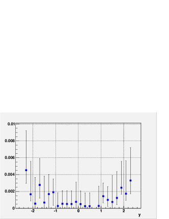
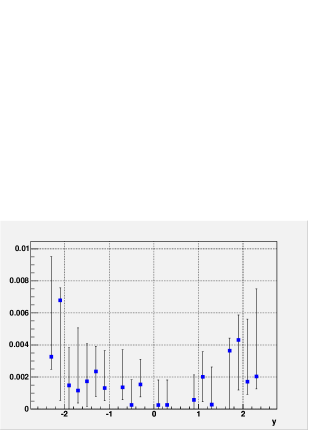
Figure 10: The rates of charge misidentification as a function of rapidity for $e^{-}$ misidentified as $e^{+}$ (left), $e^{+}$ misidentifed as $e^{-}$ (right).

2.3.5 Compare events at the generator level to events at the detector level

We have simulated one million signal, $W\rightarrow e\nu_{e}$, events for each of the PDF sets CTEQ6.1, MRST2001 and ZEUS-S using HERWIG (6.505). For each of these PDF sets the eigenvector error PDF sets have been simulated by PDF reweighting and k-factors have been applied to approximate an NLO generation. The top part of Fig. 11 shows the $e^{\pm}$ and $A_{l}$ spectra at this generator level, for all of the PDF sets superimposed. The events are then passed through the ATLFAST fast simulation of the ATLAS detector. This applies loose kinematic cuts: $|\eta|<2.5$, $p_{te}>5$ GeV, and electron isolation criteria. It also smears the 4-momenta of the leptons to mimic momentum dependent detector resolution. We then apply the selection cuts described in Sec. 2.3.3. The lower half of Fig. 11 shows the $e^{\pm}$ and $A_{l}$ spectra at the detector level after application of these cuts, for all of the PDF sets superimposed. The level of precision of each PDF set, seen in the analytic calculations of Fig. 6, is only slightly degraded at detector level, so that a net level of PDF uncertainty at central rapidity of $\sim 8\%$ is maintained. The anticipated cancellation of PDF uncertainties in the asymmetry spectrum is also observed, within each PDF set, and the spread between PDF sets suggests that measurements which are accurate to better than $\sim 5\%$ could discriminate between PDF sets.

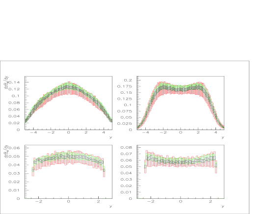
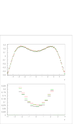
Figure 11: Top row: $e^{-}$, $e^{+}$ and $A_{e}$ rapidity spectra for the lepton from the $W$ decay, generated using HERWIG + k factors and CTEQ6.1 (red), ZEUS-S (green) and MRST2001 (black) PDF sets with full uncertainties. Bottom row: the same spectra after passing through the ATLFAST detector simulation and selection cuts.

2.3.6 Using LHC data to improve precision on PDFs

The high cross-sections for $W$ production at the LHC ensure that it will be the experimental systematic errors, rather than the statistical errors, which are determining. We have imposed a random $4\%$ scatter on our samples of one million $W$ events, generated using different PDFs, in order to investigate if measurements at this level of precision will improve PDF uncertainties at central rapidity significantly if they are input to a global PDF fit. Fig. 12 shows the $e^{+}$ and $e^{-}$ rapidity spectra for events generated from the ZEUS-S PDFs ($|\eta|<2.4$) compared to the analytic predictions for these same ZEUS-S PDFs. The lower half of this figure illustrates the result if these events are then included in the ZEUS-S PDF fit. The size of the PDF uncertainties, at $y=0$, decreases from $5.8\%$ to $4.5\%$. The largest improvement is in the PDF parameter $\lambda_{g}$ controlling the low-$x$ gluon at the input scale, $Q^{2}_{0}$: $xg(x)\sim x^{\lambda_{g}}$ at low-$x$, $\lambda_{g}=-0.199\pm 0.046$, before the input of the LHC pseudo-data, compared to, $\lambda_{g}=-0.196\pm 0.029$, after input. Note that whereas the relative normalisations of the $e^{+}$ and $e^{-}$ spectra are set by the PDFs, the absolute normalisation of the data is free in the fit so that no assumptions are made on our ability to measure luminosity. Secondly, we repeat this procedure for events generated using the CTEQ6.1 PDFs. As shown in Fig. 13, the cross-section for these events is on the lower edge of the uncertainty band of the ZEUS-S predictions. If these events are input to the fit the central value shifts and the uncertainty decreases. The value of the parameter $\lambda_{g}$ becomes, $\lambda_{g}=-0.189\pm 0.029$, after input of these pseudo-data. Finally to simulate the situation which really faces experimentalists we generate events with CTEQ6.1, and pass them through the ATLFAST detector simulation and cuts. We then correct back from detector level to generator level using a different PDF set- in this case the ZEUS-S PDFs- since in practice we will not know the true PDFs. Fig. 14 shows that the resulting corrected data look pleasingly like CTEQ6.1, but they are more smeared. When these data are input to the PDF fit the central values shift and errors decrease just as for the perfect CTEQ6.1 pseudo-data. The value of $\lambda_{g}$ becomes, $\lambda=-0.181\pm 0.030$, after input of these pseudo-data. Thus we see that the bias introduced by the correction procedure from detector to generator level is small compared to the PDF uncertainty.

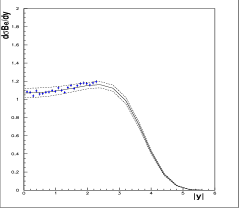
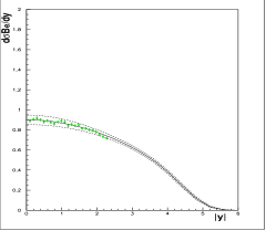
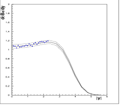
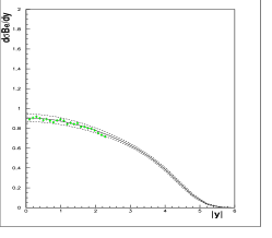
Figure 12: Top row: $e^{+}$ and $e^{-}$ rapidity spectra generated from ZEUS-S PDFs compared to the analytic prediction using ZEUS-S PDFs. Bottom row: the same lepton rapidity spectra compared to the analytic prediction AFTER including these lepton pseudo-data in the ZEUS-S PDF fit.

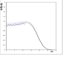
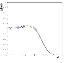
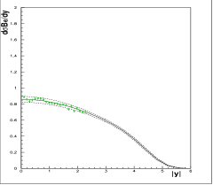
Figure 13: Top row: $e^{+}$ and $e^{-}$ rapidity spectra generated from CTEQ6.1 PDFs compared to the analytic prediction using ZEUS-S PDFs. Bottom row: the same lepton rapidity spectra compared to the analytic prediction AFTER including these lepton pseudo-data in the ZEUS-S PDF fit.

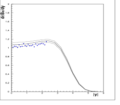
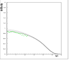
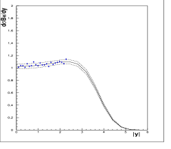
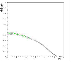
Figure 14: Top row: $e^{+}$ and $e^{-}$ rapidity spectra generated from CTEQ6.1 PDFs, which have been passed through the ATLFAST detector simulation and corrected back to generator level using ZEUS-S PDFs, compared to the analytic prediction using ZEUS-S PDFs. Bottom row: the same lepton rapidity spectra compared to the analytic prediction AFTER including these lepton pseudo-data in the ZEUS-S PDF fit.

2.3.7 Conclusions and a warning: problems with the theoretical predictions at small-$x$?

We have investigated the PDF uncertainty on the predictions for $W$ and $Z$ production at the LHC, taking into account realistic expectations for measurement accuracy and the cuts on data which will be needed to identify signal events from background processes. We conclude that at the present level of PDF uncertainty the decay lepton asymmetry, $A_{l}$, will be a useful standard model benchmark measurement, and that the decay lepton spectra can be used as a luminosity monitor which will be good to $\sim 8\%$. However, we have also investigated the measurement accuracy necessary for early measurements of these decay lepton spectra to be useful in further constraining the PDFs. A systematic measurement error of less than $\sim 4\%$ would provide useful extra constraints.

However, a caveat is that the current study has been performed using standard PDF sets which are extracted using NLO QCD in the DGLAP [24, 25, 26, 27] formalism. The extension to NNLO is straightforward, giving small corrections $\sim 1\%$. PDF analyses at NNLO including full accounting of the PDF uncertainties are not extensively available yet, so this small correction is not pursued here. However, there may be much larger uncertainties in the theoretical calculations because the kinematic region involves low-$x$. There may be a need to account for $ln(1/x)$ resummation (first considered in the BFKL [28, 29, 30] formalism) or high gluon density effects. See reference [31] for a review.

The MRST group recently produced a PDF set, MRST03, which does not include any data for $x<5\times 10^{-3}$. The motivation behind this was as follows. In a global DGLAP fit to many data sets there is always a certain amount of tension between data sets. This may derive from the use of an inappropriate theoretical formalism for the kinematic range of some of the data. Investigating the effect of kinematic cuts on the data, MRST found that a cut, $x>5\times 10^{-3}$, considerably reduced tension between the remaining data sets. An explanation may be the inappropriate use of the DGLAP formalism at small-$x$. The MRST03 PDF set is thus free of this bias BUT it is also only valid to use it for $x>5\times 10^{-3}$. What is needed is an alternative theoretical formalism for smaller $x$. However, the MRST03 PDF set may be used as a toy PDF set, to illustrate the effect of using very different PDF sets on our predictions. A comparison of Fig. 15 with Fig. 3 or Fig. 6 shows how different the analytic predictions are from the conventional ones, and thus illustrates where we might expect to see differences due to the need for an alternative formalism at small-$x$.

Figure 15: LHC $W^{+},W^{-},Z$ rapidity distributions for the MRST03 PDFs: left plot $W^{+}$; middle plot $W^{-}$; right plot $Z$

2.4 $W$ and $Z$ production at the LHC

The study of the production at the LHC of the electroweak bosons $W$ and $Z$ with subsequent decays in leptonic final states will provide several precision measurements of Standard Model parameters such as the mass of the $W$ boson or the weak mixing angle from the $Z$ boson forward-backward asymmetry. Given their large cross section and clean experimental signatures, the bosons will furthermore serve as calibration tool and luminosity monitor. More challenging, differential cross sections in rapidity or transverse momentum may be used to further constrain parton distribution functions. Eventually these measurements for single inclusive boson production may be applied to boson pair production in order to derive precision predictions for background estimates to discovery channels like $H\rightarrow W^{+}W^{-}$.

This contribution is devoted to the estimation of current uncertainties in the calculations for Standard Model cross sections involving $W$ and $Z$ bosons with particular emphasis on the PDF and perturbative uncertainties. All results are obtained at NLO with MCFM [32] version 4.0 interfaced to LHAPDF [17] for a convenient selection of various PDF families and evaluation of their intrinsic uncertainties. The cross sections are evaluated within a typical experimental acceptance and for momentum cuts summarised in Table 3. The electromagnetic decays of $W$ and $Z$ are considered (massless leptons) and the missing transverse energy is assigned to the neutrino momentum sum (in case of $W$ decays).

Table 3: Experimental acceptance cuts used for the calculation of cross-sections.

Observable	cut
$p_{T}^{lept}$	$>25$ GeV
$p_{T}^{jet}$	$>25$ GeV
$|\eta_{lept}|$	$<3.0$
$|\eta_{jet}|$	$<4.0$
$R(lepton-jet)$	$>0.8$
$R(lepton-lepton)$	$>0.2$
$E_{T}^{miss}$	$>$25 GeV

Jets in the processes $W/Z+jets$ are produced in an inclusive mode with at least one jet in the event reconstructed with the $k_{T}$-algorithm. MCFM includes one- and two-jet processes at NLO and three-jet processes at LO. In the case of boson pair production the cuts of Table 3 can only be applied to the two leading leptons, hence a complete acceptance is assumed for additional leptons e.g. from $ZZ$ or $WZ$ decays.

The calculations with MCFM are carried out for a given fixed set of electroweak input parameters using the effective field theory approach [32]. The PDF family CTEQ61 provided by the CTEQ collaboration [33] is taken as nominal PDF input while MRST2001E given by the MRST group [34] is considered for systematic purposes. The difference between CTEQ61 and MRST2001E alone can’t be considered as systematic uncertainty but merely as cross-check. The systematic uncertainty is therefore estimated for each family separately with the family members, 40 for CTEQ61 and 30 for MRST2001E, which are variants of the nominal PDF obtained with different assumptions while maintaining a reasonable fit of the input data. The value of $\alpha_{s}$ is not a free input parameter for the cross section calculation but taken from the corresponding value in the PDF.

Important input parameters are renormalisation and factorisation scales. The central results are obtained with $\mu_{R}=\mu_{F}=M_{V}$, $V=W,Z$ for single boson production and $\mu_{R}=\mu_{F}=M_{V}+M_{V}^{\prime}$ for pair production ($V^{\prime}$ being the second boson in the event). Missing higher orders are estimated by a variation of the scales in the range $1/2\leq x_{\mu R}\leq 2$ and independently $1/2\leq x_{\mu F}\leq 2$ where $\mu=x_{\mu}\cdot M_{V}$, following prescriptions applied to other processes [35], keeping in mind that the range of variation of the scales is purely conventional.

2.4.1 Single $W$ and $Z$ cross sections

Detailed studies of single $W$ and $Z$ production including detector simulation are presented elsewhere in these proceedings, here these channels are mainly studied for comparison with the associated production with explicitly reconstructed jets and with pair production. The selected process is inclusive in the sense that additional jets, present in the NLO calculation, are not explicitly reconstructed. The experimentally required lepton isolation entailing a jet veto in a restricted region of phase space is disregarded at this stage.

As an example the pseudo-rapidity distribution of the lepton from $W$ decays and the $p_{T}$ spectra for $Z$ and $W^{+}$ are shown in fig. 16.

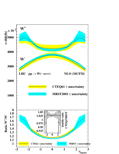
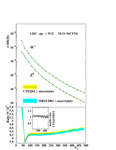
Figure 16: Left: pseudo-rapidity distribution of the decay lepton from inclusive $W$ production and right: $p_{T}$ spectra of $W$ and $Z$. The bands represent the PDF-uncertainty. The lower inserts show on the left side the ratio $W^{+}/W^{-}$ resp. the double-ratio CTEQ/MRST and on the right side the ratios for $W^{+}/Z^{0}$.

The cross section for $W^{+}$ is larger than for $W^{-}$ as a direct consequence of the difference between up- and down-quark PDFs, and this difference survives in the pseudo-rapidity distribution of the decay lepton with a maximum around $|\eta|$=2.5. In the central part the PDF uncertainty, represented by the bands in fig. 16, amounts to about 5$\%$ for CTEQ and 2$\%$ for MRST, and within the uncertainty CTEQ and MRST are fully consistent. Larger differences are visible in the peaks for the $W^{+}$, where at the same time the PDF uncertainty increases. In the ratio $W^{+}/W^{-}$ the PDF uncertainty is reduced to about 1-2$\%$ in the central region and a difference of about 3$\%$ is observed between CTEQ and MRST, as can be seen from the double-ratio CTEQ/MRST. The uncertainty of the double ratio is calculated from the CTEQ uncertainty band alone.

In the case of $Z$ production the rapidity and $p_{T}$ spectra can be fully reconstructed from the $e^{+}e^{-}$ pair. A measurement of the $Z$ $p_{T}$ spectrum may be used to tune the Monte Carlo description of $W$ $p_{T}$, which is relevant for measurements of the $W$ mass. The $p_{T}$ spectra are shown in the right part of fig. 16. The total yield for $W^{+}$ is about six times larger than for $Z^{0}$ but for $p_{T}>150$ GeV the ratio stabilises around 4.5. At small values of $p_{T}$ the fixed-order calculation becomes trustless and should be supplemented by resummed calculations. The PDF uncertainties for the $p_{T}$ spectra themselves are again about 5$\%$ and about 2$\%$ in the ratio, CTEQ and MRST being consistent over the entire $p_{T}$ range.

The perturbative uncertainties are estimated by variations of the renormalisation and factorisation scales in by a factor of two. The scale variation entails a global change in the total cross section of the order of 5$\%$. The $\eta$ distribution of leptons from $W/Z$ decays are shown in fig. 17, comparing the nominal cross section with $x_{\mu R}=x_{\mu F}=1$, to alternative scale settings. The nominal cross section is drawn with its PDF uncertainty band, illustrating that the perturbative uncertainties are of the same size. For $W^{-}$ and $Z^{0}$ the shape of the distribution is essentially unaltered, but for $W^{+}$ the region around the maxima is changed more than the central part, leading to a shape deformation. The scale variation uncertainty is strongly correlated for $W^{-}$ and $Z^{0}$ and cancels in the ratio $W^{-}/Z^{0}$, but for $W^{+}$ it is almost anti-correlated with $W^{-}$ and $Z^{0}$ and partly enhanced in the ratio.

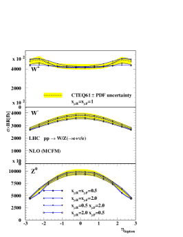
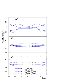
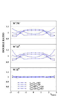
Figure 17: Left: pseudo-rapidity distribution of the decay lepton from inclusive $W/Z$ production for different values of $x_{\mu R}$ and $x_{\mu F}=1$, centre: the ratio of predictions with respect to $x_{\mu}=1$ and right: double ratio $V/V^{\prime}$ of cross sections for actual scale settings normalised to the nominal scale.

Globally the perturbative uncertainty is dominated by the asymmetric scale setting $x_{\mu R}=2,x_{\mu R}=1/2$ for which a change of $-5\%$ is observed, the largest upward shift of $3.5\%$ is obtained for $x_{\mu R}=2,x_{\mu R}=2$, locally the uncertainty for $W^{+}$ can be much different. It can be expected that the perturbative uncertainties are reduced for NNLO calculations to the level of $1\%$.

The integrated cross sections and systematic uncertainties within the experimental acceptance are summarised in Table 4.

Table 4: Total cross-sections and systematic uncertainties within the experimental acceptance.

	$W^{+}$	$W^{-}$	$Z^{0}$
CTEQ61 [pb]	5438	4002	923.9
$\Delta_{PDF}^{CTEQ}$ [pb]	$\pm 282$	$\pm 221$	$\pm 49.1$
$\Delta_{PDF}^{CTEQ}$ [$\%$]	$\pm 5.2$	$\pm 5.5$	$\pm 5.3$
MRST [pb]	5480	4110	951.1
$\Delta_{PDF}^{MRST}$ [pb]	$\pm 103$	$\pm 83.4$	$\pm 17.4$
$\Delta_{PDF}^{MRST}$ [$\%$]	$\pm 1.9$	$\pm 2.1$	$\pm 1.9$
$\Delta_{pert}$ [$\%$]	$+3.5$	$+3.5$	$+3.1$
	$-5.2$	$-5.4$	$-5.5$

2.4.2 $W/Z+jet$ production

In the inclusive production of $W/Z+jet$ at least one jet is requested to be reconstructed, isolated from any lepton by $R>0.8$. Additional jets are in case of overlap eventually merged at reconstruction level by the $k_{T}$-prescription. Given the presence of a relatively hard ($p_{T}>25$ GeV) jet, it can be expected that PDF- and perturbative uncertainties are different than for single boson production. The study of this process at the LHC, other than being a stringent test of perturbative QCD, may in addition contribute to a better understanding of the gluon PDF.

The first difference with respect to single boson production appears in the lepton pseudo-rapidities, shown in fig. 18. The peaks in the lepton spectrum from $W^{+}$ disappeared, the corresponding spectrum from $W^{-}$ is stronger peaked at central rapidity while the ratio $W^{+}/W^{-}$ with jets is essentially the same as without jets. The PDF uncertainties are slightly smaller (4.2-4.4$\%$) compared to single bosons. The jet pseudo-rapidities are shown in the right part of fig. 18, they are much stronger peaked in the central region but the ratio $W^{+}/W^{-}$ for jets is similar to the lepton ratio.

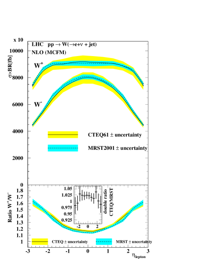
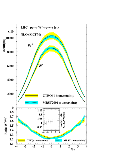
Figure 18: Left: pseudo-rapidity distribution of the decay lepton from inclusive $W$+jet production and right: pseudo-rapidity of the associated leading jet. The bands represent the PDF-uncertainty.

The transverse momenta of associated jets from $W/Z+jet$ production is shown in fig. 19, the spectra are steeply falling and the ratio $W^{+}/W^{-}$ is increasing from $1.3$ at low $p_{T}$ to almost 2 at 500 GeV $p_{T}$.

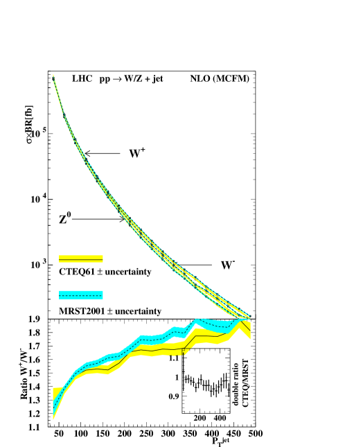
Figure 19: Transverse momentum distribution of the jet from inclusive $W/Z+jet$ production

The perturbative uncertainties are investigated in the same way as for the single boson production and are shown in fig. 20. The scale variation entails here a much larger uncertainty between 8 and 10$\%$, almost twice as large as for single bosons. In contrast to the latter case, the scale variation is correlated for $W$ and $Z$ and cancels in the ratio $W^{+}/W^{-}$, with an exception for $W^{-}$ where a bump appears at $|\eta|=1.8$ for $x_{\mu R}=2$.

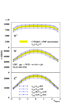
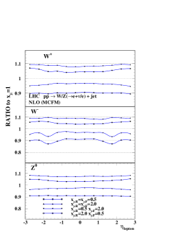
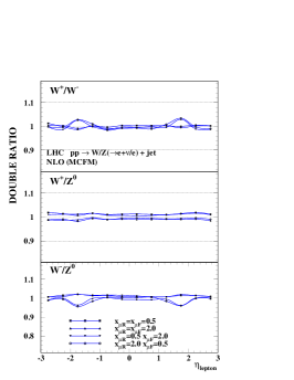
Figure 20: Left: pseudo-rapidity distribution of the decay lepton from inclusive $W/Z+jet$ production for different values of $x_{\mu R}$ and $x_{\mu F}=1$, centre: the ratio of predictions with respect to $x_{\mu}=1$ and right: double ratio $V/V^{\prime}$ of cross sections for actual scale settings normalised to the nominal scale.

The total cross sections and their systematic uncertainties are summarised in Table 5.

Table 5: Total cross-sections and systematic uncertainties within the experimental acceptance for $W/Z+jet$ processes.

	$W^{+}+jet$	$W^{-}+jet$	$Z^{0}+jet$
CTEQ61 [pb]	1041	784.5	208.1
$\Delta_{PDF}^{CTEQ}$ [pb]	$\pm 44.1$	$\pm 34.3$	$\pm 9.01$
$\Delta_{PDF}^{CTEQ}$ [$\%$]	$\pm 4.2$	$\pm 4.4$	$\pm 4.3$
MRST [pb]	1046	797.7	211.3
$\Delta_{PDF}^{MRST}$ [pb]	$\pm 17.6$	$\pm 14.8$	$\pm 3.67$
$\Delta_{PDF}^{MRST}$ [$\%$]	$\pm 1.7$	$\pm 1.9$	$\pm 1.8$
$\Delta_{pert}$ [$\%$]	$+8.7$	$+8.9$	$+7.6$
	$-9.8$	$-10.0$	$-9.1$

2.4.3 Vector Boson pair production

In the Standard Model the non-resonant production of vector bosons pairs in the continuum is suppressed by factors of $10^{4}$-$10^{5}$ with respect to single Boson production. The cross sections for $WW$, $WZ$ and $ZZ$ within the experimental acceptance range from 500 fb ($WW$) to 10 fb ($ZZ$). Given the expected limited statistics for these processes, the main goal of their experimental study is to obtain the best estimate of the background they represent for searches of the Higgs boson or new physics yielding boson pairs.

The selection of boson pairs follows in extension the single boson selection cuts applied to 2, 3 or 4 isolated leptons. Again real gluon radiation and virtual loops have been taken into account at NLO but without applying lepton-jet isolation cuts. Lepton-lepton separation is considered only for the two leading leptons.

The pseudo-rapidity and transverse momentum distributions taking the $e^{+}$ from $W^{+}W^{-}$ production as example are shown in fig.21. The pseudo-rapidity is strongly peaked and the cross section at $\eta=0$ twice as large as at $|\eta|=3$. The PDF uncertainties are smaller than for single bosons, between 3.5 and 4 $\%$.

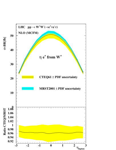
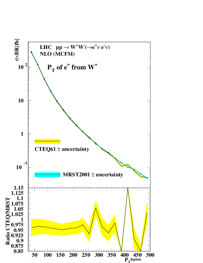
Figure 21: Left: pseudo-rapidity distribution of the decay lepton from inclusive $WW$ production and right: transverse momentum of the decay lepton.

The same shape of lepton distributions is also found for the other lepton and for the other pair production processes, as shown for the $W^{-}Z^{0}$ case in fig.22.

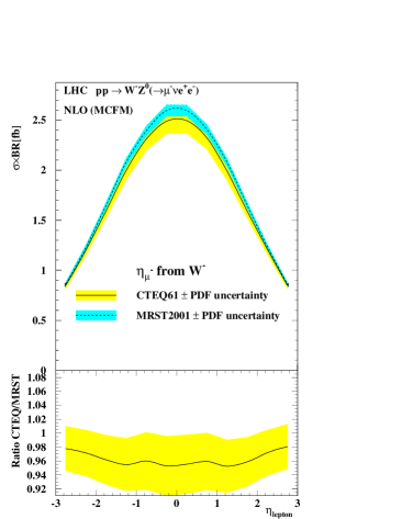
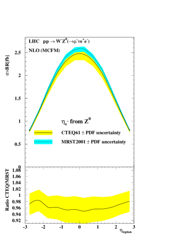
Figure 22: Left: pseudo-rapidity distribution of the decay lepton of the $W^{-}$from inclusive $W^{-}Z^{0}$ production and right: pseudo-rapidity distribution of a decay lepton of the $Z^{0}$.

The rapidity distribution of the leading $Z^{0}$ from $ZZ$ production is shown in the left part of fig.23. With both $Z$’s being fully reconstructed, the invariant mass of the $ZZ$ system can be compared in the right part of fig.23 to the invariant mass spectrum of the Higgs decaying into the same final state for an intermediate mass of $m_{H}=200$ GeV. In this case a clear peak appears at low invariant masses above the continuum, and the mass spectrum is also harder at high masses in presence of the Higgs.

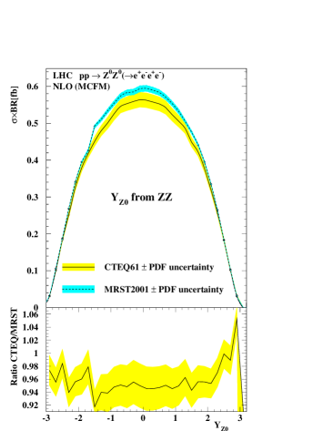
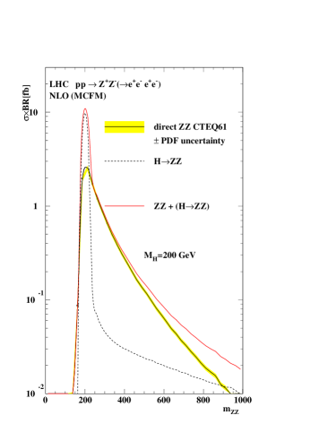
Figure 23: Left: rapidity distribution of the leading $Z$ from inclusive $ZZ$ production and right: invariant mass of the $ZZ$ pair for non-resonant continuum production compared to resonant pair production via the SM Higgs decay.

The perturbative uncertainties, obtained as for the other processes, are shown in fig.24 for the lepton distributions. The systematic uncertainties range from 3.3 to 4.9 $\%$ and are slightly smaller than for single bosons, given the larger scale $\mu=2M_{V}$ and better applicability of perturbative QCD. The perturbative uncertainty is essentially constant across the pseudo-rapidity and largely correlated between different pair production processes.

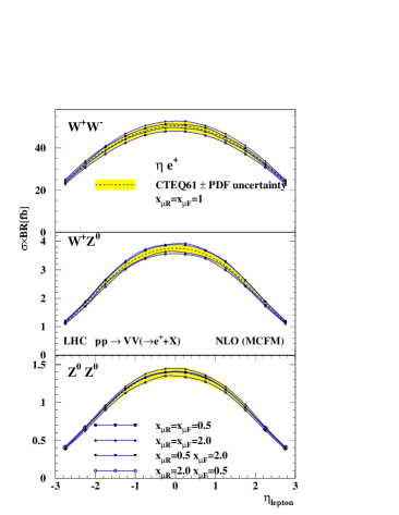
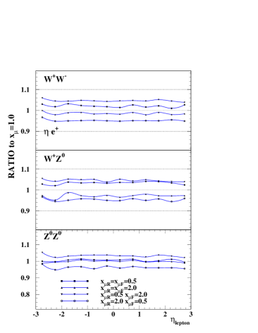
Figure 24: Left: pseudo-rapidity distributions of leptons from various boson pair production processes and different scale settings and right: ratio of predictions relative to $x_{\mu}=1$.

The ratio of boson pair production to single $Z$ production is of particular interest, as similar quark configurations contribute to both process types, though evidently in a somewhat different $x,Q^{2}$ regime. This ratio is shown in fig.25 for the lepton distribution, given the different shapes of pseudo-rapidity is not flat but its PDF uncertainty is reduced to the level of 2 $\%$. The perturbative uncertainties of the $VV/Z$ ratio, however, are only reduced for the $ZZ/Z$ case and even slightly larger for other ratios because the scale variations have partly an opposite effect on the cross sections for $Z$ and e.g. $WW$ production.

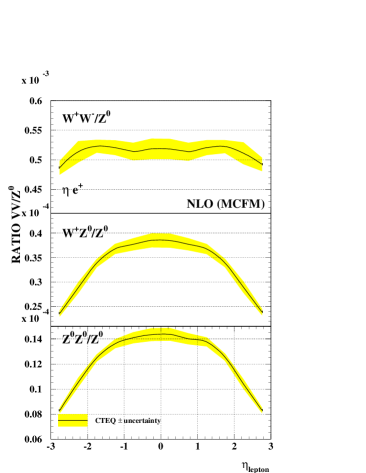
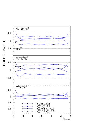
Figure 25: Left: the ratio of pseudo-rapidity distributions of leptons from boson pair production processes normalised to single $Z$ production and right: the double ratio $VV/Z$ of predictions for different scales relative to $x_{\mu}=1$.

The total cross sections and their systematic uncertainties are summarised in Table 6.

Table 6: Total cross-sections and systematic uncertainties within the experimental acceptance for pair production processes.

	$WW$	$ZZ$	$W^{+}Z^{0}$	$W^{-}Z^{0}$
CTEQ61 [fb]	475.7	11.75	31.81	20.77
$\Delta_{PDF}^{CTEQ}$ [fb]	$\pm 17.0$	$\pm 0.48$	$\pm 1.12$	$\pm 0.80$
$\Delta_{PDF}^{CTEQ}$ [$\%$]	$\pm 3.6$	$\pm 4.1$	$\pm 3.5$	$\pm 3.8$
MRST [fb]	494.2	12.34	32.55	21.62
$\Delta_{PDF}^{MRST}$ [fb]	$\pm 6.3$	$\pm 0.19$	$\pm 0.49$	$\pm 0.41$
$\Delta_{PDF}^{MRST}$ [$\%$]	$\pm 1.3$	$\pm 1.6$	$\pm 1.5$	$\pm 1.9$
$\Delta_{pert}$ [$\%$]	$+4.6$	$+3.3$	$+4.6$	$+4.8$
	$-4.9$	$-3.8$	$-4.7$	$-4.7$

2.5 Study of next-to-next-to-leading order QCD predictions for W and Z production at LHC

It has been in 2004 that the first differential next-to-next-to-leading order (NNLO) QCD calculation for vector boson production in hadron collisions was completed by Anastasiou et al. [36]. This group has calculated the rapidity dependence for W and Z production at NNLO. They have shown that the perturbative expansion stabilizes at this order in perturbation theory and that the renormalization and factorization scale uncertainties are drastically reduced, down to the level of one per-cent. It is therefore interesting to perform a more detailed study of these NNLO predictions for various observables which can be measured at LHC, as well as to investigate their systematic uncertainties.

In the study presented here we have calculated both the differential (in rapidity) and inclusive cross sections for W, Z and high-mass Drell-Yan (Z/$\gamma^{*}$) production. Here ”inclusive” refers to the results obtained by integrating the differential cross sections over a rapidity range similar to the experimentally accessible region, which might be more relevant than the complete cross section which also includes the large-rapidity tails.

Such a prediction would then be compared to the experimental measurements at LHC, which will allow for precise tests of the Standard Model as well as to put strong constraints on the parton distribution functions (PDFs) of the proton. It is clear that in the experiment only the rapidity and transverse momenta of the leptons from the vector boson decays will be accessible, over a finite range in phase space. In order to compute the rapidity of the vector boson by taking into account the finite experimental lepton acceptance, Monte Carlo simulations have to be employed which model vector boson production at the best possible precision in QCD, as for example the program MC@NLO [21]. The so computed acceptance corrections will include further systematic uncertainties, which are not discussed here.

2.5.1 Parameters and analysis method

The NNLO predictions have been implemented in the computer code VRAP [37], which has been modified in order to include ROOT [38] support for producing ntuples, histograms and plots. The code allows to specify the collision energy (14 TeV in our case), the exchanged vector boson ($\gamma^{*},\mathrm{Z}$, $\mathrm{Z}/\gamma^{*}$, $\mathrm{W}^{+}$, $\mathrm{W}^{-}$), the scale $Q$ of the exchanged boson ($M_{\mathrm{Z}},M_{\mathrm{W}}$ or off-shell, e.g.  $Q=400\,\mathrm{GeV}$), the renormalization and factorization scales, the invariant mass of the di-lepton system (fixed or integrated over a specified range), the value of the electro-magnetic coupling ($\alpha_{\mathrm{QED}}=1/128$ or $\alpha_{\mathrm{QED}}(Q)$) and the number of light fermions considered. Regarding the choice of pdfs, the user can select a pdf set from the MRST2001 fits [39] or from the ALEKHIN fits [40], consistent at NNLO with variable flavour scheme. We have chosen the MRST2001 NNLO fit, mode 1 with $\alpha_{s}(M_{\mathrm{Z}})=0.1155$ [39], as reference set.

The program is run to compute the differential cross section $d\sigma/dY$, $Y$ being the boson rapidity, at a fixed number of points in $Y$. This result is then parametrized using a spline interpolation, and the thus found function can be integrated over any desired rapidity range, such as $|Y|<2,|Y|<2.5$ or $|Y|<3$, as well as over finite bins in rapidity. For the study of on-shell production the integration range over the di-lepton invariant mass $M_{ll}$ was set to $M_{V}-3\Gamma_{V}<M_{ll}<M_{V}+3\Gamma_{V}$, with $M_{V}$ and $\Gamma_{V}$ the vector boson mass and width. This simulates an experimental selection over a finite signal range.

The systematic uncertainties have been divided into several categories: The PDF uncertainty is estimated by taking the maximum deviation from the reference set when using different PDFs from within the MRST2001 set or the ALEKHIN set. The latter difference is found to give the maximal variation in all of the investigated cases. The renormalization and factorization scales $\mu=\mu_{\mathrm{R}},\mu_{\mathrm{F}}$ have been varied between $0.5<\mu/Q<2$, both simultaneously as well as fixing one to $\mu=Q$ and varying the other. The maximum deviation from the reference setting $\mu=Q$ is taken as uncertainty. The observed difference when using either a fixed or a running electro-magnetic coupling constant is also studied as possible systematic uncertainty due to higher-order QED effects. Since it is below the one per-cent level, it is not discussed further. Finally, in the case of Z production it has been checked that neglecting photon exchange and interference contributions is justified in view of the much larger PDF and scale uncertainties.

2.5.2 Results for W and Z production

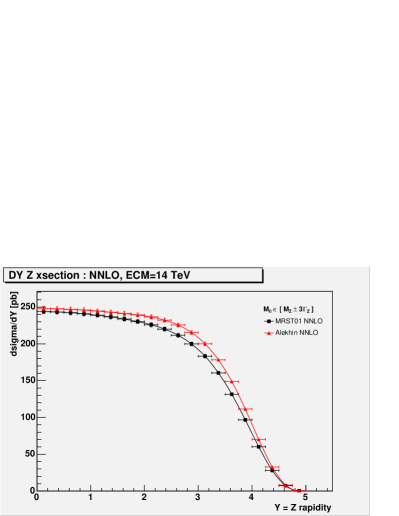
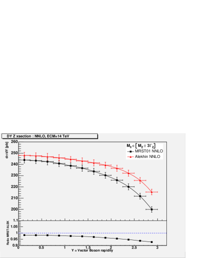
Figure 26: Left : Drell-Yan Z production cross section ($\times$ BR) at LHC energies, as a function of the Z rapidity, for two different PDF choices. Right : Zoom into a restricted rapidity region, with the ratio of the predictions for the two different PDF sets as lower inset. The error bars indicate the scale uncertainties.

In Figure 26 the results for Z production at LHC are shown for two different choices of PDF set, as a function of the boson rapidity. It can be seen that the predictions differ by about 2% at central rapidity, and the difference increases to about 5% at large rapidity. A similar picture is obtained when integrating the differential cross section up to rapidities of 2, 2.5 and 3 (Table 7). The more of the high-rapidity tail is included, the larger the uncertainty due to the PDF choice. From Table 1 it can also be seen that the scale uncertainties are slightly below the one per-cent level. It is worth noting that the choice of the integration range over the di-lepton invariant mass can have a sizeable impact on the cross section. For example, increasing the range from the standard value to $66\,\mathrm{GeV}<M_{\mathrm{Z}}<116\,\mathrm{GeV}$ increases the cross section by 8%.

Channel	Z prod.			W prod.
range	$|Y|<2$	$|Y|<2.5$	$|Y|<3$	$|Y|<2$	$|Y|<2.5$	$|Y|<3$
cross section [nb]	0.955	1.178	1.384	9.388	11.648	13.800
$\Delta$ PDF [%]	2.44	2.95	3.57	5.13	5.47	5.90
$\Delta$ scale [%]	0.85	0.87	0.90	0.99	1.02	1.05

Table 7: NNLO QCD results for W and Z production at the LHC for the integration over different rapidity ranges. Also given are the relative uncertainties due to the choice of the PDFs and of the renormalization and factorization scale. The numbers include the branching ratio $Z(W)\rightarrow ee(e\nu)$.

The results for W production (Table 7) have been obtained by first calculating separately the cross sections for $\mathrm{W}^{+}$ and $\mathrm{W}^{-}$ production, and then adding these up. Again we observe an increase of the PDF uncertainty when going to larger rapidity ranges. Compared to the Z production, here the PDF uncertainties are larger, between 5 and 6%, whereas the scale uncertainties are of the same level, $\approx 1\%$. It is interesting to note that the PDF uncertainty for $\mathrm{W}^{-}$ production is about 10 - 20% (relative) lower than that for $\mathrm{W}^{+}$.

A considerable reduction in systematic uncertainty can be obtained by calculating cross section ratios. Two options have been investigated, namely the ratios $\sigma(\mathrm{W}^{+})/\sigma(\mathrm{W}^{-})$ and $\sigma(\mathrm{W})/\sigma(\mathrm{Z})$. As can be seen from Figure 27, the PDF uncertainties are reduced to the 0.7% level in the former ratio, and to about 2% in the latter. The scale uncertainties are reduced to the 0.15% level in both cases. Taking such ratios has also the potential advantage of reduced experimental systematic uncertainties, such as those related to the acceptance corrections.

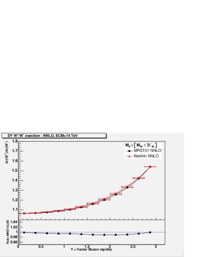
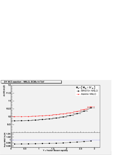
Figure 27: Ratio of the production cross sections for $\mathrm{W}^{+}$, $\mathrm{W}^{-}$ (left), and W, Z (right), as a function of rapidity, for two different PDF sets. The inserts show the ratios of the results for the two PDF choices.

2.5.3 Results for high-mass Drell-Yan processes

Similarly to on-shell W and Z production we have also analyzed the high-mass Drell-Yan process, namely $\mathrm{Z}/\gamma^{*}$ production at a scale of $Q=400$ GeV. In this case the di-lepton invariant mass has been integrated over the range $M_{ll}=400\pm 50$ GeV. Here the PDF uncertainties are found between 3.7% and 5.1% for the various integration ranges over rapidity, somewhat larger than for on-shell production. However, by normalizing the high-mass production cross section to the on-shell case, the PDF uncertainties are considerably reduced, being 1.2 - 1.5%.

The systematic uncertainties related to the renormalization and factorization scale are reduced ($\Delta$ scale $\approx 0.2\%$) when going to the high-mass exchange, as expected from perturbative QCD with a decreasing strong coupling constant. In this case a normalization of the cross section to the on-shell case does not give an improvement. However, since the scale uncertainties are well below the PDF uncertainties, this is less of an issue for the moment.

2.5.4 Summary

We have studied NNLO QCD predictions for W and Z production at LHC energies. We have identified the choice of PDF set as the dominant systematic uncertainty, being between 3 and 6%. The choice of the renormalization and factorization scale leads to much smaller uncertainties, at or below the 1% level. In particular we have shown that the systematic uncertainties can be sizeably reduced by taking ratios of cross sections, such as $\sigma(\mathrm{W}^{+})/\sigma(\mathrm{W}^{-})$, $\sigma(\mathrm{W})/\sigma(\mathrm{Z})$ or $\sigma(\mathrm{Z}/\gamma^{*},Q=400\,\mathrm{GeV})$/$\sigma(\mathrm{Z}/\gamma^{*},Q=M_{\mathrm{Z}})$. For such ratios it can be expected that also part of the experimental uncertainties cancel. With theoretical uncertainties from QCD at the few per-cent level the production of W and Z bosons will most likely be the best-known cross section at LHC.

Concerning the next steps, it should be considered that at this level of precision it might become relevant to include also higher-order electro-weak corrections. In addition, since experimentally the boson rapidity will be reconstructed from the measured lepton momenta, a detailed study is needed to evaluate the precision at which the acceptance correction factors for the leptons from the boson decays can be obtained. For this Monte Carlo programs such as MC@NLO should be employed, which combine next-to-leading-order matrix elements with parton showers and correctly take account of spin correlations.

3 Experimental determination of Parton Distributions

3.1 Introduction

With HERA currently in its second stage of operation, it is possible to assess the potential precision limits of HERA data and to estimate the potential impact of the measurements which are expected at HERA-II, in particular with respect to the PDF uncertainties.

Precision limits of the structure function analyses at HERA are examined in section 3.2. Since large amounts of luminosity are already collected, the systematic uncertainty becomes most important. A detailed study of error sources with particular emphasis on correlated errors for the upcoming precision analysis of the inclusive DIS cross section at low $Q^{2}$ using 2000 data taken by the H1 experiment is presented. A new tool, based on the ratio of cross sections measured by different reconstruction methods, is developed and its ability to qualify and unfold various correlated error sources is demonstrated.

An important issue is the consistency of the HERA data. In section 3.3, the H1 and ZEUS published PDF analyses are compared, including a discussion of the different treatments of correlated systematic uncertainties. Differences in the data sets and the analyses are investigated by putting the H1 data set through both PDF analyses and by putting the ZEUS and H1 data sets through the same (ZEUS) analysis, separately. Also, the HERA averaged data set (section 3.4) is put through the ZEUS PDF analysis and the result is compared to that obtained when putting the ZEUS and H1 data sets through this analysis together, using both the Offset and Hessian methods of treating correlated systematic uncertainties.

The HERA experimental data can not only be cross checked with respect to each other but also combined into one common dataset, as discussed in section 3.4. In this respect, a method to combine measurements of the structure functions performed by several experiments in a common kinematic domain is presented. This method generalises the standard averaging procedure by taking into account point-to-point correlations which are introduced by the systematic uncertainties of the measurements. The method is applied to the neutral and charged current DIS cross section data published by the H1 and ZEUS collaborations. The averaging improves in particular the accuracy due to the cross calibration of the H1 and ZEUS measurements.

The flavour decomposition of the light quark sea is discussed in section 3.6. For low $x$ and thus low $Q^{2}$ domain at HERA only measurement of the photon exchange induced structure functions $F_{2}$ and $F_{L}$ is possible, which is insufficient to disentangle individual quark flavours. A general strategy in this case is to assume flavour symmetry of the sea. Section 3.6 considers PDF uncertainties if this assumption is released. These uncertainties can be significantly reduced if HERA would run in deuteron-electron collision mode.

The impact of projected HERA-II data on PDFs is estimated in section 3.7. In particular, next-to-leading order (NLO) QCD predictions for inclusive jet cross sections at the LHC centre-of-mass energy are presented using the estimated PDFs. A further important measurement which could improve understanding of the gluon density at low $x$ and, at the same time, provide consistency checks of the low $Q^{2}$ QCD evolution is the measurement of the longitudinal structure function $F_{L}$. Perspectives of this measurement are examined in section 3.5, while the impact of this measurement is also estimated in section 3.7.

Further improvements for consistently including final-state observables in global QCD analyses are discussed in section 3.8. There, a method for “a posteriori” inclusion of PDFs, whereby the Monte Carlo run calculates a grid (in $x$ and $Q$) of cross section weights that can subsequently be combined with an arbitrary PDF. The procedure is numerically equivalent to using an interpolated form of the PDF. The main novelty relative to prior work is the use of higher-order interpolation, which substantially improves the tradeoff between accuracy and memory use. An accuracy of about $0.01$% has been reached for the single inclusive cross-section in the central rapidity region $|y|<0.5$ for jet transverse momenta from $100$ to $5000\mathrm{GeV}$. This method will make it possible to consistently include measurements done at HERA, Tevatron and LHC in global QCD analyses.

3.2 Precision Limits for HERA DIS Cross Section Measurement

The published precision low $Q^{2}$ cross section data [41] of the H1 experiment became an important data set in various QCD fit analyses [41, 18, 19, 40]. Following success of these data the H1 experiment plans to analyse a large data sample, taken during 2000 running period, in order to reach precision limits of low $Q^{2}$ inclusive cross sections measurements at HERA. The precision is expected to approach 1% level.

The aim of this contribution is to calculate realistic error tables for 2000 H1 data and pursue paths how to reach such a high precision. Correlated error sources are studied in particular and a new tool, based on the ratio of cross sections measured by different reconstruction methods, is developed. All errors, including correlated errors, are treated in the same manner as in [41]. Error tables are provided and used in QCD fit analysis, see Sec 3.7, in order to study the impact of the new data on PDFs. The new data are expected to reach higher precision level than [41] due to the following reasons

• Larger data statistics - Statistical errors will decrease by factor of $1.5-2$, compared to [41], depending on the kinematic region.

• Very large Monte Carlo simulations (MC) - Due to a progress in computing a number of simulated events can be significantly increased in order to minimise statistical error of MC, to understand uncorrelated errors and to estimate correlated errors more precisely.

• During past years increasing knowledge, arriving from various H1 analyses, enabled better understanding of the detector and its components as well as improving quality of MC.

• Data taking in 2000 was particularly smooth. Both HERA and H1 were running at peak performance for HERA-I running period.

This contribution uses existing 2000 data and MC ntuples along with the full analysis chain. It applies all preliminary technical work done on these data, including calibration, alignment, trigger studies etc. Quoted errors are assumed to be achieved in the final version of analysis yet the analysis has not been finalised, all the numbers in the paper are preliminary and may change in the publication.

The uncertainties of the cross section measurement are divided into a number of different types. Namely, these are statistical uncertainties of the data, uncorrelated systematics and correlated systematics. The term ’correlated’ refers to the fact that cross section measurements in kinematic bins are affected in a correlated way while different correlated systematic error sources are considered uncorrelated among each other. The classification of the systematic errors into types is sometimes straightforward (MC statistics is uncorrelated error source) but sometimes is rather arbitrary (radiative corrections are assumed to be uncorrelated error source). The main goal of this classification is to preserve correlation between data points while keeping the treatement as simple as possible.

The cross section uncertainties depend on the method used to reconstruct event kinematics. There are various methods existing, involving a measurement of the scattered electron as well as of the hadronic finale state. In the following two of them, so called electron method and sigma method, are employed [42]. The electron method uses only the measurement of the scattered electron, namely its energy and polar angle, while the sigma method uses both the scattered electron and the hadronic final state. An advantage of the sigma method is a proper treatment of QED radiation from the incoming beam electron (ISR).

The statistical uncertainty of the data is typically 0.5-1%, depending on the kinematic region analysed and the definition of the kinematic bins. In the following we adapt the bin definition used in [41], apart from merging bins at low $y$ which was done in the published data in order to increase statistics.

The uncorrelated systematics consists from various contributions. A cross section uncertainty due to the Monte Carlo statistics is the one with very good potential to be minimised. In the following we assume 100 million simulated events to be used in analysis of 2000 data. Estimates were calculated with available 12 million simulated events and corresponding statistical errors scaled by a factor of $\sqrt{100/12}$. As a result the uncertainty is very small and typically on the level of few permile.

Additional contributions to the uncorrelated systematics are efficiencies. We assume for trigger efficiency 0.3% and backward tracker tracker efficiency 0.3% uncertainty. Radiative corrections are expected to affect the final cross section by 0.4%.

Effect of correlated uncertainties on the cross section measurement is studied in the following manner. Particular source of correlated uncertainty, for instance the scattered electron energy measurement, is varied by assumed error and the change of the measured cross section is quoted as the corresponding cross section measurement error. An example of cross section change on various correlated error source is shown in Fig. 28 for bin of $Q^{2}=45\,{\rm GeV}^{2}$ and $x=0.005$. The kinematics of events was reconstructed with the sigma method (a) and the electron method (b). Errors are calculated as so called standard errors of the mean in calculation of which the available Monte Carlo sample was split into nine sub-samples. It is clearly seen that the cross section measurement with the sigma method in this kinematic bin is particularly sensitive to the electron energy measurement (top-left) and to noise description in LAr calorimeter (bottom-right). On the contrary, the electron polar angle measurement and the calibration of the hadronic final state play a little role. The electron method is mainly sensitive to the electron energy measurement. The importance of the systematic sources vary from bin to bin.

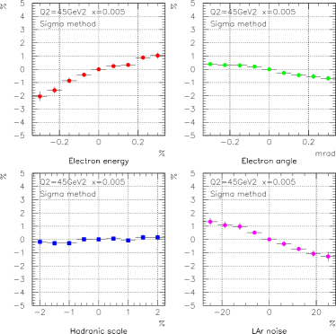
a)       b)

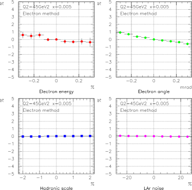
Figure 28: A scan of the cross section measurement change in % depending on a variation of (from top-left) electron energy, electron polar angle, hadronic final state calibration scale and noise level in LAr calorimeter (bottom-right). The sigma method (a) and the electron method (b) were used to reconstruct kinematics of events.

There are five individual sources contributing to the correlated cross section uncertainties:

• Uncertainties of 0.15% at $E_{e}=27\,$GeV and 1% at 7 GeV are assigned to the electron energy scale for the backward calorimeter. The uncertainty is treated as a linear function of $E_{e}$ interpolating between the results at 27 GeV and 7 GeV.

• The uncertainty on the scattered electron polar angle measurement is 0.3 mrad . The corresponding error on the cross section measurement is typically well below 1% but may be larger at lowest values of $Q^{2}$.

• The uncertainty on the hadronic energy scale comprises a number of systematic error sources corresponding to the $E-p_{z}$ decomposition: an uncertainty of the hadronic energy scale calibration of 2% for the central and forward calorimeter, an uncertainty of 3% for the fraction carried by tracks and a 5% uncertainty of the hadronic energy scale measured in backward calorimeter.

• The uncertainty on the hadronic energy scale is further affected by the subtracted noise in the calorimetery. The noise is described to the level of 10% and the corresponding error is propagated to the cross section uncertainty. The largest influence is in the low $y$ region, which is measured with the sigma method.

• The uncertainty due to the photoproduction background at large $y$ is estimated from the normalisation error of the PHOJET simulations to about 10%. At low and medium values of $y\lesssim 0.5$ it is negligible.

The total systematic error is calculated from the quadratic summation over all sources of the uncorrelated and correlated systematic uncertainties. The total error of the DIS cross section measurement is obtained from the statistical and systematical errors added in quadrature.

Table 8: An example of the error table for $Q^{2}=25\,{\rm GeV}^{2}$ for 2000 data, large Monte Carlo sample and suppressed systematic errors compared to [1], see text for details. Absolute errors are shown. The table format is identical to the one published in [1].

Table 9: An example of the full error table for $Q^{2}=25\,{\rm GeV}^{2}$, published H1 data. The definition of kinematic bins is not identical to that in Table 8, some bins were merged to enlarge statistics.

An example of the full error table for kinematic bin of $Q^{2}=25\,{\rm GeV}^{2}$ is shown in Table 8. For a comparison the corresponding part of the published data from [41] is presented in Table 9. One can see that precision about 1% can be reached especially in four lowest $x$ bins, where the electron method was used to reconstruct the event kinematics. The key contributions to the seen improvement in the cross section measurement precision are the electron energy measurement, very large Monte Carlo statistics, well understood noise in LAr calorimeter and precisely controlled efficiencies entering the analysis.

Full error table, covering the kinematic region of $5\leq Q^{2}\leq 150\,{\rm GeV}^{2}$ and $0.01\leq y\leq 0.6$ was produced. The electron method was applied for kinematic bins at $y>0.1$ while the sigma method otherwise. The measurement of the proton structure function $F_{2}$ was simulated using fractal parametrisation [43] for central values, accounting for all sources of correlated and uncorrelated errors. This table was used to estimate effect of precise low $Q^{2}$ data on the determination of proton PDFs from QCD fits.

The fact that different kinematics reconstruction methods are affected differently by the correlated systematic uncertainties may be employed as a tool to estimate these uncertainties. We define

$$R_{i}=\frac{\sigma_{r}^{el,i}}{\sigma_{r}^{\Sigma,i}}$$ (2)

to be the cross section measurement ratio, where the reduced cross section $\sigma_{r}^{el,i}$ and $\sigma_{r}^{\Sigma,i}$ is measured using the electron method and the sigma method, respectively. Kinematic bins, indexed by $i$, cover a region of the analysis phase space where both reconstruction methods are applicable for the measurement. The statistical error of $R_{i}$ measurement is again evaluated by splitting the sample to a number of sub-samples and calculating the standard error of the mean. An example of a scan of the cross section ratio $R_{i}$ dependence on the hadronic final state calibration variation in a bin of $Q^{2}=25\,{\rm GeV}^{2}$ and various inelasticity $y$ is shown in Fig. 29.

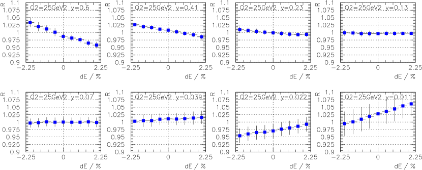
Figure 29: A scan of the cross section ratio R in bins of $Q^{2}$ and $y$ as a function of the hadronic final state calibration variation.

An error of a particular correlated uncertainty source $j$ can be estimated by searching for lowest $\chi^{2}=\sum_{i}(R_{i}(\alpha_{j})-1)^{2}/\sigma^{2}_{i}$, where summation runs over kinematic bins, $\sigma_{i}$ is the error of $R_{i}$ measurement and $\alpha_{j}$ is the variation of the source $j$. However, since there is a number of correlated error sources the correct way to find correlated uncertainties is account for all of them.

Unfolding of the correlated error sources can be linearised and directly solved by minimising the following function:

$${\cal L}=\sum_{i}\frac{1}{\sigma_{i}^{2}}(R_{i}+\sum_{j}\alpha_{j}\frac{\partial R_{i}}{\partial\alpha_{j}}-1)^{2}.$$ (3)

The partial derivatives $\frac{\partial R_{i}}{\partial\alpha_{j}}$ for systematic source $\alpha_{j}$ are obtained from linear fits to distributions as shown in Fig. 29. Parameters $\alpha_{j}$ and their respective errors are obtained by matrix inversion technique.

The procedure was tested on available Monte Carlo sample for 2000 H1 data. Half of the sample, six million events, was used to simulate data. Full analysis chain was applied to measure the cross section and thus $R_{i}$. Kinematic bins were selected according to $15\leq Q^{2}\leq 60\,{\rm GeV}^{2}$ and $0.011\leq y\leq 0.6$, i.e. in the main region of the data. The results are shown in Fig. 30. Closed points correspond to unfolded errors of the electron energy measurement (top-left), hadronic final state calibration and noise in the LAr calorimeter (bottom-left). There is no sensitivity observed to the electron polar angle measurement. All values are within statistical errors compatible with zero, as expected. For the final analysis the statistical errors are expected to be approximately three times smaller due to the significantly larger statistics than used for the presented study. This will enable the method to gain sufficient control over systematic correlated errors. Apart from being able to evaluate calibration of the scattered electron and of the hadronic final state, it gives a very good handle on the LAr calorimeter noise.

For a comparison, open points in Fig. 30 correspond to a $\chi^{2}$ scan in one correlated error source. The statistical errors are smaller, as expected, and compatible with zero. However, the unfolding method is preferred since it takes into account all correlated error sources correctly.

In summary, a study of the DIS cross section uncertainties realistically achievable at HERA has been performed. For $x\in 0.001-0.01$ a precision of $1\%$ can be reached across for a wide range of $Q^{2}\in 5-150$ GeV², allowing improved estimate of $W,Z$ production cross section in the central rapidity region of LHC. The accuracy of the DIS cross section measurement can be verified using different kinematic reconstruction methods available at the HERA collider.

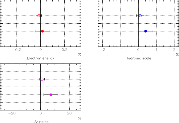
Figure 30: Errors on the electron energy measurement (top-left), hadronic scale calibration (top-right) and noise in LAr calorimeter (bottom-left). Open points correspond to $\chi^{2}$ scan in one correlated error source. Closed points show the result of complete unfolding, taking into account correlations.

3.3 Comparison and combination of ZEUS and H1 PDF analyses

Parton Density Function (PDF) determinations are usually global fits [19, 18, 45], which use fixed target DIS data as well as HERA data. In such analyses the high statistics HERA NC $e^{+}p$ data, which span the range $6.3\times 10^{-5}<x<0.65,2.7<Q^{2}<30,000$GeV², have determined the low-$x$ sea and gluon distributions, whereas the fixed target data have determined the valence distributions and the higher-$x$ sea distributions. The $\nu$-Fe fixed target data have been the most important input for determining the valence distributions, but these data suffer from uncertainties due to heavy target corrections. Such uncertainties are also present for deuterium fixed target data, which have been used to determine the shape of the high-$x$ $d$-valence quark.

HERA data on neutral and charged current (NC and CC) $e^{+}p$ and $e^{-}p$ inclusive double differential cross-sections are now available, and have been used by both the H1 and ZEUS collaborations [46, 47] in order to determine the parton distributions functions (PDFs) using data from within a single experiment. The HERA high $Q^{2}$ cross-section data can be used to determine the valence distributions, thus eliminating uncertainties from heavy target corrections. The PDFs are presented with full accounting for uncertainties from correlated systematic errors (as well as from statistical and uncorrelated sources). Peforming an analysis within a single experiment has considerable advantages in this respect, since the global fits have found significant tensions between different data sets, which make a rigorous statistical treatment of uncertainties difficult.

Fig. 31 compares the results of the H1 and ZEUS analyses. Whereas the extracted PDFs are broadly compatible within errors, there is a noticeable difference in the shape of the gluon PDFs.

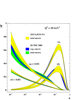
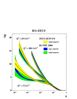
Figure 31: Left plot: Comparison of PDFs from ZEUS and H1 analyses at $Q^{2}=10$GeV². Right plot: Comparison of gluon from ZEUS and H1 analyses, at various $Q^{2}$. Note that the ZEUS analysis total uncertainty includes both experimental and model uncertainties.

Full details of the analyses are given in the relevant publications, in this contribution we examine the differences in the two analyses, recapping only salient details.

3.3.1 Comparing ZEUS and H1 published PDF analyses

The kinematics of lepton hadron scattering is described in terms of the variables $Q^{2}$, the invariant mass of the exchanged vector boson, Bjorken $x$, the fraction of the momentum of the incoming nucleon taken by the struck quark (in the quark-parton model), and $y$ which measures the energy transfer between the lepton and hadron systems. The differential cross-section for the NC process is given in terms of the structure functions by

$$\frac{d^{2}\sigma(e^{\pm}p)}{dxdQ^{2}}=\frac{2\pi\alpha^{2}}{Q^{4}x}\left[Y_{+}\,F_{2}(x,Q^{2})-y^{2}\,F_{L}(x,Q^{2})\mp Y_{-}\,xF_{3}(x,Q^{2})\right],$$ (4)

where $\displaystyle Y_{\pm}=1\pm(1-y)^{2}$. The structure functions $F_{2}$ and $xF_{3}$ are directly related to quark distributions, and their $Q^{2}$ dependence, or scaling violation, is predicted by pQCD. At $Q^{2}\leq 1000$ GeV² $F_{2}$ dominates the charged lepton-hadron cross-section and for $x\leq 10^{-2}$, $F_{2}$ itself is sea quark dominated but its $Q^{2}$ evolution is controlled by the gluon contribution, such that HERA data provide crucial information on low-$x$ sea-quark and gluon distributions. At high $Q^{2}$, the structure function $xF_{3}$ becomes increasingly important, and gives information on valence quark distributions. The CC interactions enable us to separate the flavour of the valence distributions at high-$x$, since their (LO) cross-sections are given by,

$$\frac{d^{2}\sigma(e^{+}p)}{dxdQ^{2}}=\frac{G_{F}^{2}M_{W}^{4}}{(Q^{2}+M_{W}^{2})^{2}2\pi x}x\left[(\bar{u}+\bar{c})+(1-y)^{2}(d+s)\right],$$

$$\frac{d^{2}\sigma(e^{-}p)}{dxdQ^{2}}=\frac{G_{F}^{2}M_{W}^{4}}{(Q^{2}+M_{W}^{2})^{2}2\pi x}x\left[(u+c)+(1-y)^{2}(\bar{d}+\bar{s})\right].$$

For both HERA analyses the QCD predictions for the structure functions are obtained by solving the DGLAP evolution equations [25, 24, 26, 27] at NLO in the $\overline{\rm{MS}}$ scheme with the renormalisation and factorization scales chosen to be $Q^{2}$. These equations yield the PDFs at all values of $Q^{2}$ provided they are input as functions of $x$ at some input scale $Q^{2}_{0}$. The resulting PDFs are then convoluted with coefficient functions, to give the structure functions which enter into the expressions for the cross-sections. For a full explanation of the relationships between DIS cross-sections, structure functions, PDFs and the QCD improved parton model see ref. [31].

The HERA data are all in a kinematic region where there is no sensitivity to target mass and higher twist contributions but a minimum $Q^{2}$ cut must be imposed to remain in the kinematic region where perturbative QCD should be applicable. For ZEUS this is $Q^{2}>2.5$ GeV², and for H1 it is $Q^{2}>3.5$ GeV². Both collaborations have included the sensitivity to this cut as part of their model errors.

In the ZEUS analysis, the PDFs for $u$ valence, $xu_{v}(x)$, $d$ valence, $xd_{v}(x)$, total sea, $xS(x)$, the gluon, $xg(x)$, and the difference between the $d$ and $u$ contributions to the sea, $x(\bar{d}-\bar{u})$, are each parametrized by the form

$$p_{1}x^{p_{2}}(1-x)^{p_{3}}P(x),$$ (5)

where $P(x)=1+p_{4}x$, at $Q^{2}_{0}=7$GeV². The total sea $xS=2x(\bar{u}+\bar{d}+\bar{s}+\bar{c}+\bar{b})$, where $\bar{q}=q_{sea}$ for each flavour, $u=u_{v}+u_{sea},d=d_{v}+d_{sea}$ and $q=q_{sea}$ for all other flavours. The flavour structure of the light quark sea allows for the violation of the Gottfried sum rule. However, there is no information on the shape of the $\bar{d}-\bar{u}$ distribution in a fit to HERA data alone and so this distribution has its shape fixed consistent with the Drell-Yan data and its normalisation consistent with the size of the Gottfried sum-rule violation. A suppression of the strange sea with respect to the non-strange sea of a factor of 2 at $Q^{2}_{0}$, is also imposed consistent with neutrino induced dimuon data from CCFR. Parameters are further restricted as follows. The normalisation parameters, $p_{1}$, for the $d$ and $u$ valence and for the gluon are constrained to impose the number sum-rules and momentum sum-rule. The $p_{2}$ parameter which constrains the low-$x$ behaviour of the $u$ and $d$ valence distributions is set equal, since there is no information to constrain any difference. When fitting to HERA data alone it is also necessary to constrain the high-$x$ sea and gluon shapes, because HERA-I data do not have high statistics at large-$x$, in the region where these distributions are small. The sea shape has been restricted by setting $p_{4}=0$ for the sea, but the gluon shape is constrained by including data on jet production in the PDF fit. Finally the ZEUS analysis has 11 free PDF parameters. ZEUS have included reasonable variations of these assumptions about the input parametrization in their analysis of model uncertainties. The strong coupling constant was fixed to $\alpha_{s}(M_{Z}^{2})=0.118$ [48]. Full account has been taken of correlated experimental systematic errors by the Offset Method, as described in ref [45, 49].

For the H1 analysis, the value of $Q^{2}_{0}=4$GeV², and the choice of quark distributions which are parametrized is different. The quarks are considered as $u$-type and $d$-type with different parametrizations for, $xU=x(u_{v}+u_{sea}+c)$, $xD=x(d_{v}+d_{sea}+s)$, $x\bar{U}=x(\bar{u}+\bar{c})$ and $x\bar{D}=x(\bar{d}+\bar{s})$, with $q_{sea}=\bar{q}$, as usual, and the the form of the quark and gluon parametrizations given by Eq. 5. For $x\bar{D}$ and $x\bar{U}$ the polynomial, $P(x)=1.0$, for the gluon and $xD$, $P(x)=(1+p_{4}x)$, and for $xU$, $P(x)=(1+p_{4}x+p_{5}x^{3})$. The parametrization is then further restricted as follows. Since the valence distributions must vanish as $x\to 0$, the low-$x$ parameters, $p_{1}$ and $p_{2}$ are set equal for $xU$ and $x\bar{U}$, and for $xD$ and $x\bar{D}$. Since there is no information on the flavour structure of the sea it is also necessary to set $p_{2}$ equal for $x\bar{U}$ and $x\bar{D}$. The normalisation, $p_{1}$, of the gluon is determined from the momentum sum-rule and the $p_{4}$ parameters for $xU$ and $xD$ are determined from the valence number sum-rules. Assuming that the strange and charm quark distributions can be expressed as $x$ independent fractions, $f_{s}$ and $f_{c}$, of the $d$ and $u$ type sea, gives the further constraint $p_{1}(\bar{U})=p_{1}(\bar{D})(1-f_{s})/(1-f_{c})$. Finally there are 10 free parameters. H1 has also included reasonable variations of these assumptions in their analysis of model uncertainties. The strong coupling constant was fixed to $\alpha_{s}(M_{Z}^{2})=0.1185$ and this is sufficiently similar to the ZEUS choice that we can rule it out as a cause of any significant difference. Full account has been taken of correlated experimental systematic errors by the Hessian Method, see ref. [49].

For the ZEUS analysis, the heavy quark production scheme used is the general mass variable flavour number scheme of Roberts and Thorne [50]. For the H1 analysis, the zero mass variable flavour number scheme is used. It is well known that these choices have a small effect on the steepness of the gluon at very small-$x$, such that the zero-mass choice produces a slightly less steep gluon. However, there is no effect on the more striking differences in the gluon shapes at larger $x$.

There are two differences in the analyses which are worth further investigation. The different choices for the form of the PDF parametrization at $Q^{2}_{0}$ and the different treatment of the correlated experimental uncertainties.

3.3.2 Comparing different PDF analyses of the same data set and comparing different data sets using the same PDF analysis.

So far we have compared the results of putting two different data sets into two different analyses. Because there are many differences in the assumptions going into these analyses it is instructive to consider:(i) putting both data sets through the same analysis and (ii) putting one of the data sets through both analyses. For these comparisons, the ZEUS analysis does NOT include the jet data, so that the data sets are more directly comparable, involving just the inclusive double differential cross-section data. Fig. 32 compares the sea and gluon PDFs, at $Q^{2}=10$GeV², extracted from H1 data using the H1 PDF analysis with those extracted from H1 data using the ZEUS PDF analysis. These alternative analyses of the same data set give results which are compatible within the model dependence error bands. Fig. 32 also compares the sea and gluon PDFs extracted from ZEUS data using the ZEUS analysis with those extracted from H1 data using the ZEUS analysis. From this comparison we can see that the different data sets lead to somewhat different gluon shapes even when put through exactly the same analysis. Hence the most of the difference in shape of the ZEUS and H1 PDF analyses can be traced back to a difference at the level of the data sets.

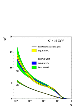
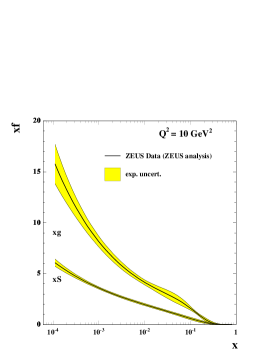
Figure 32: Sea and gluon distributions at $Q^{2}=10$GeV² extracted from different data sets and different analyses. Left plot: H1 data put through both ZEUS and H1 analyses. Middle plot: ZEUS data put through ZEUS analysis. Right plot: H1 data put through ZEUS analysis.

3.3.3 Comparing the Offset and Hessian method of assessing correlated experimental uncertainties

Before going further it is useful to discuss the treatment of correlated systematic errors in the ZEUS and H1 analyses. A full discussion of the treatment of correlated systematic errors in PDF analyses is given in ref [31], only salient details are recapped here. Traditionally, experimental collaborations have evaluated an overall systematic uncertainty on each data point and these have been treated as uncorrelated, such that they are simply added to the statistical uncertainties in quadrature when evaluating $\chi^{2}$. However, modern deep inelastic scattering experiments have very small statistical uncertainties, so that the contribution of systematic uncertainties becomes dominant and consideration of point to point correlations between systematic uncertainties is essential.

For both ZEUS and H1 analyses the formulation of the $\chi^{2}$ including correlated systematic uncertainties is constructed as follows. The correlated uncertainties are included in the theoretical prediction, $F_{i}(p,s)$, such that

$$F_{i}(p,s)=F_{i}^{\rm NLOQCD}(p)+\sum_{\lambda}s_{\lambda}\Delta^{\rm sys}_{i\lambda}$$

where, $F_{i}^{\rm NLOQCD}(p)$, represents the prediction from NLO QCD in terms of the theoretical parameters $p$, and the parameters $s_{\lambda}$ represent independent variables for each source of systematic uncertainty. They have zero mean and unit variance by construction. The symbol $\Delta^{\rm sys}_{i\lambda}$ represents the one standard deviation correlated systematic error on data point $i$ due to correlated error source $\lambda$. The $\chi^{2}$ is then formulated as

$$\chi^{2}=\sum_{i}\frac{\left[F_{i}(p,s)-F_{i}(\rm meas)\right]^{2}}{\sigma_{i}^{2}}+\sum_{\lambda}s^{2}_{\lambda}$$ (6)

where, $F_{i}(\rm meas)$, represents a measured data point and the symbol $\sigma_{i}$ represents the one standard deviation uncorrelated error on data point $i$, from both statistical and systematic sources. The experiments use this $\chi^{2}$ in different ways. ZEUS uses the Offset method and H1 uses the Hessian method.

Traditionally, experimentalists have used ‘Offset’ methods to account for correlated systematic errors. The $\chi^{2}$ is formluated without any terms due to correlated systematic errors ($s_{\lambda}=0$ in Eq. 6) for evaluation of the central values of the fit parameters. However, the data points are then offset to account for each source of systematic error in turn (i.e. set $s_{\lambda}=+1$ and then $s_{\lambda}=-1$ for each source $\lambda$) and a new fit is performed for each of these variations. The resulting deviations of the theoretical parameters from their central values are added in quadrature. (Positive and negative deviations are added in quadrature separately.) This method does not assume that the systematic uncertainties are Gaussian distributed. An equivalent (and much more efficient) procedure to perform the Offset method has been given by Pascaud and Zomer [51], and this is what is actually used. The Offset method is a conservative method of error estimation as compared to the Hessian method. It gives fitted theoretical predictions which are as close as possible to the central values of the published data. It does not use the full statistical power of the fit to improve the estimates of $s_{\lambda}$, since it choses to mistrust the systematic error estimates, but it is correspondingly more robust.

The Hessian method is an alternative procedure in which the systematic uncertainty parameters $s_{\lambda}$ are allowed to vary in the main fit when determining the values of the theoretical parameters. Effectively, the theoretical prediction is not fitted to the central values of the published experimental data, but these data points are allowed to move collectively, according to their correlated systematic uncertainties. The theoretical prediction determines the optimal settings for correlated systematic shifts of experimental data points such that the most consistent fit to all data sets is obtained. Thus, in a global fit, systematic shifts in one experiment are correlated to those in another experiment by the fit. In essence one is allowing the theory to calibrate the detectors. This requires great confidence in the theory, but more significantly, it requires confidence in the many model choices which go into setting the boundary conditions for the theory (such as the parametrization at $Q^{2}_{0}$).

The ZEUS analysis can be performed using the Hessian method as well as the Offset method and Fig. 33 compares the PDFs, and their uncertainties, extracted from ZEUS data using these two methods.

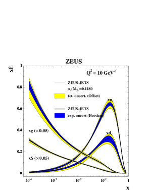
Figure 33: PDFs at $Q^{2}=10$GeV², for the ZEUS analysis of ZEUS data performed by the Offset and the Hessian methods.

The central values of the different methods are in good agreement but the use of the Hessian method results in smaller uncertainties, for a the standard set of model assumptions, since the input data can be shifted within their correlated systematic uncertainties to suit the theory better. However, model uncertainties are more significant for the Hessian method than for the Offset method. The experimental uncertainty band for any one set of model choices is set by the usual $\chi^{2}$ tolerance, $\Delta\chi^{2}=1$, but the acceptability of a different set of choices is judged by the hypothesis testing criterion, such that the $\chi^{2}$ should be approximately in the range $N\pm\surd(2N)$, where $N$ is the number of degrees of freedom. The PDF parameters obtained for the different model choices can differ by much more than their experimental uncertainties, because each model choice can result in somewhat different values of the systematic uncertainty parameters, $s_{\lambda}$, and thus a different estimate of the shifted positions of the data points. This results in a larger spread of model uncertainty than in the Offset method, for which the data points cannot move. Fig 31 illustrates the comparability of the ZEUS (Offset) total uncertainty estimate to the H1 (Hessian) experimental plus model uncertainty estimate.

Another issue which arises in relation to the Hessian method is that the data points should not be shifted far outside their one standard deviation systematic uncertainties. This can indicate inconsistencies between data sets, or parts of data sets, with respect to the rest of the data. The CTEQ collaboration have considered data inconsistencies in their most recent global fit [18]. They use the Hessian method but they increase the resulting uncertainty estimates, by increasing the $\chi^{2}$ tolerance to $\Delta\chi^{2}=100$, to allow for both model uncertainties and data inconsistencies. In setting this tolerance they have considered the distances from the $\chi^{2}$-minima of individual data sets to the global minimum for all data sets. These distances by far exceed the range allowed by the $\Delta\chi^{2}=1$ criterion. Strictly speaking such variations can indicate that data sets are inconsistent but the CTEQ collaboration take the view that all of the current world data sets must be considered acceptable and compatible at some level, even if strict statistical criteria are not met, since the conditions for the application of strict criteria, namely Gaussian error distributions, are also not met. It is not possible to simply drop “inconsistent” data sets, as then the partons in some regions would lose important constraints. On the other hand the level of “inconsistency” should be reflected in the uncertainties of the PDFs. This is achieved by raising the $\chi^{2}$ tolerance. This results in uncertainty estimates which are comparable to those achieved by using the Offset method [49].

3.3.4 Using both H1 and ZEUS data in the same PDF analysis

Using data from a single experiment avoids questions of data consistency, but to get the most information from HERA it is necessary to put ZEUS and H1 data sets into the same analysis together, and then questions of consistency arise. Fig 34 compares the sea and gluon PDFs and the $u$ and $d$ valence PDFs extracted from the ZEUS PDF analysis of ZEUS data alone, to those extracted from the ZEUS PDF analysis of both H1 and ZEUS data.

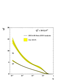
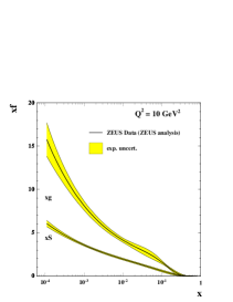
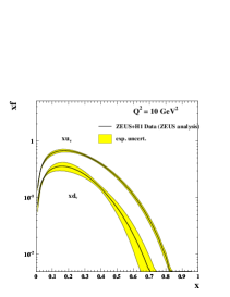
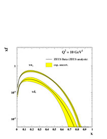
Figure 34: Top plots: Sea and gluon distributions at $Q^{2}=10$GeV² extracted from H1 and ZEUS data using the ZEUS analysis (left) compared to those extracted from ZEUS data alone using the ZEUS analysis (right). Bottom Plots: Valence distributions at $Q^{2}=10$GeV², extracted from H1 and ZEUS data using the ZEUS analysis (left) compared to those extracted from ZEUS data alone using the ZEUS analysis (right).

It is noticeable that, for the low-$x$ sea and gluon PDFs, combining the data sets does not bring a reduction in uncertainty equivalent to doubling the statistics. This is because the data which determine these PDFs are systematics limited. In fact there is some degree of tension between the ZEUS and the H1 data sets, such that the $\chi^{2}$ per degree of freedom rises for both data sets when they are fitted together. The Offset method of treating the systematic errors reflects this tension such that the overall uncertainty is not much improved when H1 data are added to ZEUS data. However, the uncertainty on the high-$x$ valence distributions is reduced by the input of H1 data, since the data are still statistics limited at high $x$.

3.3.5 Combining the H1 and ZEUS data sets before PDF analysis

Thus there could be an advantage in combining ZEUS and H1 data in a PDF fit if the tension between the data sets could be resolved. It is in this context the question of combining these data into a single data set arises. The procedure for combination is detailed in the contribution of S. Glazov to these proceedings (section 3.4). Essentially, since ZEUS and H1 are measuring the same physics in the same kinematic region, one can try to combine them using a ’theory-free’ Hessian fit in which the only assumption is that there is a true value of the cross-section, for each process, at each $x,Q^{2}$ point. The systematic uncertainty parameters, $s_{\lambda}$, of each experiment are fitted to determine the best fit to this assumption. Thus each experiment is calibrated to the other. This works well because the sources of systematic uncertainty in each experiment are rather different. Once the procedure has been performed the resulting systematic uncertainties on each of the combined data points are significantly smaller than the statistical errors. Thus one can legitimately make a fit to the combined data set in which these statistical and systematic uncertainties are simply combined in quadrature. The result of making such a fit, using the ZEUS analysis, is shown in Fig. 35.

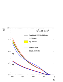
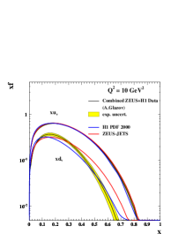
Figure 35: Left plot: Sea and gluon distributions at $Q^{2}=10$GeV², extracted from the combined H1 and ZEUS data set using the ZEUS analysis. Right plot: Valence distributions at $Q^{2}=10$GeV², extracted from the combined H1 and ZEUS data set using the ZEUS analysis.

The central values of the ZEUS and H1 published analyses are also shown for comparison. Looking back to Fig. 34 one can see that there has been a dramatic reduction in the level of uncertainty compared to the ZEUS Offset method fit to the separate ZEUS and H1 data sets. This result is very promising. A preliminary study of model dependence, varying the form of the polynomial, $P(x)$, used in the PDF paremtrizations at $Q^{2}_{0}$, also indicates that model dependence is relatively small.

The tension between ZEUS and H1 data could have been resolved by putting them both into a PDF fit using the Hessian method to shift the data points. That is, rather than calibrating the two experiments to each other in the ’theory-free’ fit, we could have used the theory of pQCD to calibrate each experiment. Fig. 36 shows the PDFs extracted when the ZEUS and H1 data sets are put through the ZEUS PDF analysis procedure using the Hessian method.

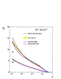
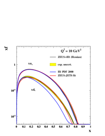
Figure 36: Left plot: Sea and gluon distributions at $Q^{2}=10$GeV², extracted from the H1 and ZEUS data sets using the ZEUS analysis done by Hessian method. Right plot: Valence distributions at $Q^{2}=10$GeV², extracted from the H1 and ZEUS data sets using the ZEUS analysis done by Hessian method.

The uncertainties on the resulting PDFs are comparable to those found for the fit to the combined data set, see Fig. 35. However, the central values of the resulting PDFs are rather different- particularly for the less well known gluon and $d$ valence PDFs. For both of the fits shown in Figs. 35, 36 the values of the systematic error parameters, $s_{\lambda}$, for each experiment have been allowed to float so that the data points are shifted to give a better fit to our assumptions, but the values of the systematic error parameters chosen by the ’theory-free’ fit and by the PDF fit are rather different. A representaive sample of these values is given in Table 10. These discrepancies might be somewhat alleviated by a full consideration of model errors in the PDF fit, or of appropriate $\chi^{2}$ tolerance when combining the ZEUS and H1 experiments in a PDF fit, but these differences should make us wary about the uncritical use of the Hessian method.

Syatematic uncertainty $s_{\lambda}$	in PDF fit	in Theory-free fit
ZEUS electron efficiency	1.68	0.31
ZEUS electron angle	-1.26	-0.11
ZEUS electron energy scale	-1.04	0.97
ZEUS hadron calorimeter energy scale	1.05	-0.58
H1 electron energy scale	-0.51	0.61
H1 hadron energy scale	-0.26	-0.98
H1 calorimeter noise	1.00	-0.63
H1 photoproduction background	-0.36	0.97

Table 10: Systematic shifts for ZEUS and H1 data as determine by a joint pQCD PDF fit, and as determined by the theory-free data combination fit

3.4 Averaging of DIS Cross Section Data

The QCD fit procedures (Alekhin [40], CTEQ [18], MRST [19], H1 [47], ZEUS [45]) use data from a number of individual experiments directly to extract the parton distribution functions (PDF). All programs use both the central values of measured cross section data as well as information about the correlations among the experimental data points.

The direct extraction procedure has several shortcomings. The number of input datasets is large containing several individual publications. The data points are correlated because of common systematic uncertainties, within and also across the publications. Handling of the experimental data without additional expert knowledge becomes difficult. Additionally, as it is discussed in Sec. 3.3, the treatment of the correlations produced by the systematic errors is not unique. In the Lagrange Multiplier method [51] each systematic error is treated as a parameter and thus fitted to QCD. Error propogation is then used to estimate resulting uncertainties on PDFs. In the so-called “offset” method (see e.g. [45]) the datasets are shifted in turn by each systematic error before fitting. The resulting fits are used to form an envelope function to estimate the PDF uncertainty. Each method has its own advantages and shortcomings, and it is difficult to select the standard one. Finally, some global QCD analyses use non-statistical criteria to estimate the PDF uncertainties ($\Delta\chi^{2}\gg 1$). This is driven by the apparent discrepancy between different experiments which is often difficult to quantify. Without a model independent consistency check of the data it might be the only safe procedure.

These drawbacks can be significantly reduced by averaging of the input structure function data in a model independent way before performing a QCD analysis of that data. One combined dataset of deep inelastic scattering (DIS) cross section measurements is much easier to handle compared to a scattered set of individual experimental measurements, while retaining the full correlations between data points. The averaging method proposed here is unique and removes the drawback of the offset method, which fixes the size of the systematic uncertainties. In the averaging procedure the correlated systematic uncertainties are floated coherently allowing in some cases reduction of the uncertainty. In addition, study of a global $\chi^{2}/dof$ of the average and distribution of the pulls allows a model independent consistency check between the experiments. In case of discrepancy between the input datasets, localised enlargement of the uncertainties for the average can be performed.

A standard way to represent a cross section measurement of a single experiment is given in the case of the $F_{2}$ structure function by:

$$\begin{array}[]{lcl}\chi^{2}_{exp}(\left\{F^{i,true}_{2}\right\},\left\{\alpha_{j}\right\})&=&\sum_{i}\frac{\textstyle\left[F_{2}^{i,true}-\left(F^{i}_{2}+\sum_{j}\frac{\partial F^{i}_{2}}{\partial\alpha_{j}}\alpha_{j}\right)\right]^{2}}{\textstyle\sigma^{2}_{i}}+\sum_{j}\frac{\textstyle\alpha^{2}_{j}}{\textstyle\sigma^{2}_{\alpha_{j}}}.\end{array}$$ (7)

Here $F^{i}_{2}$ ($\sigma^{2}_{i}$) are the measured central values (statistical and uncorrelated systematic uncertainties) of the $F_{2}$ structure function, $\alpha_{j}$ are the correlated systematic uncertainty sources and $\partial F^{i}_{2}/\partial\alpha_{j}$ are the sensitivities of the measurements to these systematic sources. Eq. 7 corresponds to the correlated probability distribution functions for the structure function $F^{i,true}_{2}$ and for the systematic uncertainties $\alpha_{j}$. Eq. 7 resembles Eq. 6 where the theoretical predictions for $F_{2}$ are substituted by $F^{i,true}_{2}$.

The $\chi^{2}$ function Eq. 7 by construction has a minimum $\chi^{2}=0$ for $F^{i,true}_{2}=F^{i}_{2}$ and $\alpha_{j}=0$. One can show that the total uncertainty for $F^{i,true}_{2}$ determined from the formal minimisation of Eq. 7 is equal to the sum in quadrature of the statistical and systematic uncertainties. The reduced covariance matrix $cov(F^{i,true}_{2},F^{j,true}_{2})$ quantifies the correlation between experimental points.

In the analysis of data from more than one experiment, the $\chi^{2}_{tot}$ function is taken as a sum of the $\chi^{2}$ functions Eq. 7 for each experiment. The QCD fit is then performed in terms of parton density functions which are used to calculate predictions for $F^{i,true}_{2}$.

Before performing the QCD fit, the $\chi^{2}_{tot}$ function can be minimised with respect to $F^{i,true}_{2}$ and $\alpha_{j}$. If none of correlated sources is present, this minimisation is equivalent to taking an average of the structure function measurements. If the systematic sources are included, the minimisation corresponds to a generalisation of the averaging procedure which contains correlations among the measurements.

Being a sum of positive definite quadratic functions, $\chi^{2}_{tot}$ is also a positive definite quadratic and thus has a unique minimum which can be found as a solution of a system of linear equations. Although this system of the equations has a large dimension it has a simple structure allowing fast and precise solution.

A dedicated program has been developed to perform this averaging of the DIS cross section data (http://www.desy.de/~glazov/f2av.tar.gz). This program can calculate the simultaneous averages for neutral current (NC) and charged current (CC) electron- and positron-proton scattering cross section data including correlated systematic sources. The output of the program includes the central values and uncorrelated uncertainties of the average cross section data. The correlated systematic uncertainties can be represented in terms of (i) covariance matrix, (ii) dependence of the average cross section on the original systematic sources together with the correlation matrix for the systematic sources, (iii) and finally the correlation matrix of the systematic sources can be diagonalised, in this case the form of $\chi^{2}$ for the average data is identical to Eq. 7 but the original systematic sources are not preserved.

Figure 37: $Q^{2}$ dependence of the NC reduced cross section for $x=0.002$ and $x=0.25$ bins. H1 data is shown as open circles, ZEUS data is shown as open squares and the average of H1 and ZEUS data is shown as filled circles. The line represents the expectation from the H1 PDF 2000 QCD fit.

The first application of the averaging program has been a determination of the average of the published H1 and ZEUS data [47, 41, 52, 53, 54, 55, 56, 57, 58, 59]. Nine individual NC and CC cross section measurements are included from H1 and seven are included from ZEUS. Several sources of systematic uncertainties are correlated between datasets, the correlations among H1 and ZEUS datasets are taken from [47] and [46], respectively. No correlations are assumed between H1 and ZEUS systematic uncertainties apart from a common $0.5\%$ luminosity measurement uncertainty. The total number of data points is 1153 (552 unique points) and the number of correlated systematic sources, including normalisation uncertainties, is 43.

The averaging can take place only if most of the data from the experiments are quoted at the same $Q^{2}$ and $x$ values. Therefore, before the averaging the data points are interpolated to a common $Q^{2},x$ grid. This interpolation is based on the H1 PDF 2000 QCD fit [47]. The interpolation of data points in principle introduces a model dependency. For H1 and ZEUS structure function data both experiments employ rather similar $Q^{2},x$ grids. About $20\%$ of the input points are interpolated, for most of the cases the correction factors are small (few percent) and stable if different QCD fit parametrizations [18, 19] are used.

The cross section data have also been corrected to a fixed center of mass energy squared $S=101570$ GeV². This has introduced a small correction for the data taken at $S=90530$ GeV². The correction is based on H1-2000 PDFs, it is only significant for high inelasticity $y>0.6$ and does not exceed $6\%$.

The HERA data sets agree very well: $\chi^{2}/dof$ for the average is $521/601$. The distribution of pulls does not show any significant tensions across the kinematic plane. Some systematic trends can be observed at low $Q^{2}<50$ GeV², where ZEUS NC data lie systematically higher than the H1 data, although this difference is within the normalisation uncertainty. An example of the resulting average DIS cross section is shown in Fig. 37, where the data points are displaced in $Q^{2}$ for clarity.

A remarkable side feature of the averaging is a significant reduction of the correlated systematic uncertainties. For example the uncertainty on the scattered electron energy measurement in the H1 backward calorimeter is reduced by a factor of three. The reduction of the correlated systematic uncertainties thus leads to a significant reduction of the total errors, especially for low $Q^{2}<100$ GeV², where systematic uncertainties limit the measurement accuracy. For this domain the total errors are often reduced by a factor two compared to the total errors of the individual H1 and ZEUS measurements.

The reduction of the correlated systematic uncertainties is achieved since the dependence of the measured cross section on the systematic sources is significantly different between H1 and ZEUS experiments. This difference is due mostly to the difference in the kinematic reconstruction methods used by the two collaborations, and to a lesser extent to the individual features of the H1 and ZEUS detectors. For example, the cross section dependence on the scattered electron energy scale has a very particular behaviour for H1 data which relies on kinematic reconstruction using only the scattered electron in one region of phase space. ZEUS uses the double angle reconstruction method where the pattern of this dependence is completely different leading to a measurement constraint.

In summary, a generalised averaging procedure to include point-to-point correlations caused by the systematic uncertainties has been developed. This averaging procedure has been applied to H1 and ZEUS DIS cross section data. The data show good consistency. The averaging of H1 and ZEUS data leads to a significant reduction of the correlated systematic uncertainties and thus a large improvement in precision for low $Q^{2}$ measurements. The goal of the averaging procedure is to obtain HERA DIS cross section set which takes into account all correlations among the experiments.

3.5 The longitudinal structure function $F_{L}$

3.5.1 Introduction

At low $x$ the sea quarks are determined by the accurate data on $F_{2}(x,Q^{2})\>$. The charm contribution to $F_{2}\,$is directly measured while there is no separation of up and down quarks at low $x$ which are assumed to have the same momentum distribution, see Sect. 3.6. Within this assumption, and setting the strange sea to be a fraction of the up/down sea, the proton quark content at low $x$ is determined. The gluon distribution $xg(x,Q^{2})\,$, however, is determined only by the derivative $\partial F_{2}/\partial\ln Q^{2}\,$ which is not well measured [41]. It is thus not surprising that rather different gluon distributions are obtained in global NLO analyses, as is illustrated in Figure 38. The figure displays the result of recent fits by MRST and CTEQ on the gluon distribution at low and high $Q^{2}$. It can be seen that there are striking differences at the initial scale, $Q^{2}=5$ GeV², which at high $Q^{2}$ get much reduced due to the evolution mechanism. The ratio of these distributions, however, exhibits differences at lower $x$ at the level of 10% even in the LHC Higgs and $W$ production kinematic range, see Figure 39. One also observes a striking problem at large $x$ which is beyond the scope of this note, however. In a recent QCD analysis it was observed [41] that the dependence of the gluon distribution at low $x$, $xg\propto x^{b_{G}}$, is correlated to the value of $\alpha_{s}(M_{Z}^{2})\,$, see Figure 40.

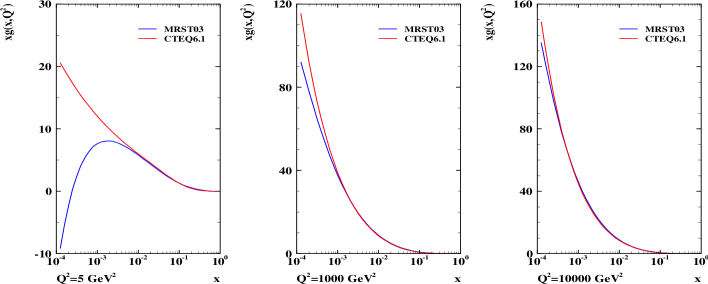
Figure 38: Gluon momentum distributions determined by MRST and CTEQ in NLO QCD, as a function of $x$ for $Q^{2}=5$ GeV², close to the initial scale of the fits, and at higher $Q^{2}$ as the result of the DGLAP evolution.

In the Quark-Parton Model the longitudinal structure function $F_{L}(x,Q^{2})\>$is zero [60]. In DGLAP QCD, to lowest order, $F_{L}\,$is given by [61]

$$F_{L}(x,Q^{2})=\frac{\alpha_{s}}{4\pi}x^{2}\int_{x}^{1}\frac{dz}{z^{3}}\cdot\left[\frac{16}{3}F_{2}(z,Q^{2})+8\sum e_{q}^{2}\left(1-\frac{x}{z}\right)zg(z,Q^{2})\right]$$ (8)

with contributions from quarks and from gluons. Approximately this equation can be solved [62] and the gluon distribution appears as a measurable quantity,

$$xg(x)=1.8[\frac{3\pi}{2\alpha_{s}}F_{L}(0.4x)-F_{2}(0.8x]\simeq\frac{8.3}{\alpha_{s}}F_{L},$$ (9)

determined by measurements of $F_{2}\,$and $F_{L}\,$. Since $F_{L}\,$, at low $x$, is not much smaller than $F_{2}\,$, to a good approximation $F_{L}\,$is a direct measure for the gluon distribution at low $x$.

Figure 39: Ratio of the gluon distributions of CTEQ to MRST as a function of $x$ for low and large $Q^{2}$.

Apart from providing a very useful constraint to the determination of the gluon distribution, see also Sect. 3.7, a measurement of $F_{L}(x,Q^{2})\>$is of principal theoretical interest. It provides a crucial test of QCD to high orders. A significant departure of an $F_{L}\,$measurement from the prediction which is based on the measurement of $F_{2}(x,Q^{2})\>$and $\partial F_{2}/\partial\ln Q^{2}\,$ only, would require theory to be modified. There are known reasons as to why the theoretical description of gluon radiation at low $x$ may differ from conventional DGLAP evolution: the neglect of $\ln(1/x)$, in contrast to BFKL evolution, or the importance of NLL resummation effects on the gluon splitting function (see Sect. 5.3). Furthermore recent calculations of deep inelastic scattering to NNLO predict very large effects from the highest order on $F_{L}\,$contrary to $F_{2}\,$[63].

Within the framework of the colour dipole model there exists a testable prediction for $F_{L}(x,Q^{2})\>$, and the longitudinal structure function, unlike $F_{2}\,$, may be subject to large higher twist effects [64].

Figure 40: Correlation of the low $x$ behaviour of the gluon distribution, characterised by the power $x^{-b_{g}}$, with the strong coupling constant $\alpha_{s}$ as obtained in the H1 NLO QCD fit to H1 and BCDMS data.

3.5.2 Indirect Determinations of $F_{L}$ at Low $x$

So far first estimates on $F_{L}(x,Q^{2})\>$at low $x$ have been obtained by the H1 Collaboration. These result from data on the inclusive $ep\rightarrow eX$ scattering cross section

$$\frac{Q^{4}x}{2\pi\alpha^{2}Y_{+}}\cdot\frac{d^{2}\sigma}{dxdQ^{2}}=[F_{2}(x,Q^{2})-f(y)\cdot F_{L}(x,Q^{2})]=\sigma_{r}$$ (10)

obtained at fixed, large energy, $s=4E_{e}E_{p}$. The cross section is defined by the two proton structure functions, $F_{2}\,$and $F_{L}\,$, with $Y_{+}=1+(1-y)^{2}$ and $f(y)=y^{2}/Y_{+}$. At fixed $s$ the inelasticity $y$ is fixed by $x$ and $Q^{2}$ as $y=Q^{2}/sx$. Thus one can only measure a combination $F_{2}-f(y)F_{L}$. Since HERA accesses a large range of $y$, and $f(y)$ is large only at large $y>0.4$, assumptions have been made on $F_{L}\,$to extract $F_{2}\,$at larger $y$. Since the cross section measurement accuracy has reached the few per cent level [41], the effect of the $F_{L}\,$assumption on $F_{2}\,$at lowest $x$ has been non-negligible. The determination of $F_{2}(x,Q^{2})\>$has thus been restricted to a region in which $y<0.6$. The proton structure function $F_{2}(x,Q^{2})\>$is known over a few orders of magnitude in $x$ rather well, from HERA and at largest $x$ from fixed target data. Thus H1 did interpret the cross section at higher $y$ as a determination of $F_{L}(x,Q^{2})\>$imposing assumptions about the behaviour of $F_{2}(x,Q^{2})\>$at lowest $x$. These were derived from QCD fits to the H1 data [65] or at lower $Q^{2}$, where QCD could not be trusted, from the derivative of $F_{2}\,$[66]. Recently, with the established $x$ behaviour [67] of $F_{2}(x,Q^{2})=c(Q^{2})x^{-\lambda(Q^{2})}$, a new method [66] has been used to determine $F_{L}\,$. This “shape method” is based on the observation that the shape of $\sigma_{r}$, Eq. 10, at high $y$ is driven by $f\propto y^{2}$ and sensitivity to $F_{L}\,$is restricted to a very narrow range of $x$ corresponding to $y=0.3-0.9$. Assuming that $F_{L}(x,Q^{2})\>$in this range, for each bin in $Q^{2}$, does not depend on $x$, one obtains a simple relation, $\sigma_{r}=cx^{-\lambda}-fF_{L}$. which has been used to determine $F_{L}(x,Q^{2})\>$.

Figure 41: Data on the longitudinal structure function obtained using assumptions on the behaviour of the other structure function $F_{2}$ in comparison with NLO QCD fit predictions. The data labeled svtx00 and mb99 data are preliminary.

Figure 41 shows the existing, preliminary data on $F_{L}(x,Q^{2})\>$at low $Q^{2}$ from the H1 Collaboration in comparison with predictions from NLO DGLAP QCD fits to HERA and further cross section data. One can see that the accuracy and the $x$ range of these $F_{L}(x,Q^{2})\>$determinations are rather limited although the data have some discriminative power already.

3.5.3 Backgrounds and Accuracy

The longitudinal structure function contribution to $\sigma_{r}$ represents a small correction of the cross section in a small part of the kinematic range only. The demands for the $F_{L}\,$measurement are extremely high: the cross section needs to be measured at the per cent level and the scattered electron be uniquely identified up to high $y$. The method of unfolding $F_{2}\,$and $F_{L}\,$consists in a measurement of $\sigma_{r}$ at fixed $x$ and $Q^{2}$ with varying $s$. This allows both structure functions to be determined from a straight line variation of $\sigma_{r}$ as a function of $f(y)$, see [68].

At large $y$, corrresponding to low $x$, and low $Q^{2}$ the scattering kinematics at HERA resembles that of a fixed target scattering experiment: the electron scattered off quarks at very low $x$ (“at rest”) is going in the backward detector region, i.e. in the direction of the electron beam. The scattered electron is accompanied by part of the hadronic final state which is related to the struck quark. High inelasticities $y\simeq 1-E_{e}^{\prime}/E_{e}$ demand to identify scattered electrons down to a few GeV of energy $E_{e}^{\prime}$. Thus a considerable background is to be isolated and removed which stems from hadrons or photons, from the $\pi_{0}\rightarrow\gamma\gamma$ decay. These particles may originate both from a genuine DIS event but to a larger extent stem from photoproduction processes, in which the scattered electron escapes mostly non recognised in electron beam direction. Removal of this background in H1 is possible by requiring a track associated to the Spacal cluster, which rejects photons, and by measuring its charge which on a statistical basis removes the remaining part of the background as was demonstrated before [41, 66].

The scattered electron kinematics, $E_{e}^{\prime}$ and $\theta_{e}$, can be accurately reconstructed using the high resolution Spacal calorimeter energy determination and the track measurements in the Backward Silicon Tracker (BST) and the Central Jet Drift Chamber (CJC). Reconstruction of the hadronic final state allows the energy momentum constraint to be imposed, using the “$E-p_{z}$” cut, which removes radiative corrections, and the Spacal energy scale to be calibrated at large $E_{e}^{\prime}$ using the double angle method. At low energies $E_{e}^{\prime}$ the Spacal energy scale can be calibrated to a few % using the $\pi_{0}$ mass constraint and be cross checked with the BST momentum measurement and with QED Compton events. The luminosity is measured to 1-2%. Any common normalisation uncertainty may be removed, or further constrained, by comparing cross section data at very low $y$ where the contribution of $F_{L}\,$is negligible.

Subsequently two case studies are presented which illustrate the potential of measuring $F_{L}\,$directly in unfolding it from the large $F_{2}\,$contribution to the cross section, a study using a set of 3 low proton beam energies and a simulation for just one low $Ep$ data set combined with standard 920 GeV data. Both studies use essentially the same correlated systematic errors and differ slightly in the assumptions on the background and efficiency uncertainties which regard the errors on cross section ratios. The following assumptions on the correlated systematics are used: $\delta E_{e}^{\prime}/E_{e}^{\prime}=0.003$ at large $E_{e}$ linearly rising to $0.03$ at 3 GeV; $\delta\theta_{e}=0.2$ mrad in the BST acceptance region and 1 mrad at larger angles; $\delta E_{h}/E_{h}=0.02$. These and further assumed systematic uncertainties represent about the state of analysis reached so far in inclusive low $Q^{2}$ cross section measurements of H1.

3.5.4 Simulation Results

A simulation has been performed for $E_{e}=27.6$ GeV and for four different proton beam energies, $E_{p}=920,\,575,\,465$ and $400\,$GeV assuming luminosities of 10, 5, 3 and 2 pb${}^{-1}\,$, respectively. The beam energies are chosen such that the cross section data are equidistant in $f(y)$. If the luminosity scales as expected as $E_{p}^{2}$, the low $E_{p}$ luminosities are equivalent to 35 pb${}^{-1}\,$at standard HERA settings. Further systematic errors regard the residual radiative corrections, assumed to be 0.5%, and the photoproduction background, 1-2% depending on $y$. This assumption on the background demands an improvement by a factor of about two at high $y$ which can be expected from a high statistics subtraction of background using the charge assignment of the electron scattering candidate. An extra uncorrelated efficiency correction is assumed of 0.5%. The resulting cross section measurements are accurate to 1-2%. For each $Q^{2}$ and $x$ point this choice provides up to four cross section measurements. The two structure functions are then obtained from a fit to $\sigma_{r}=F_{2}+f(y)F_{L}$ taking into account the correlated systematics. This separation provides also accurate data of $F_{2}$, independently of $F_{L}\,$. The simulated data on $F_{L}\,$span nearly one order of magnitude in $x$ and are shown in Figure 42. For the chosen luminosity the statistical and systematic errors on $F_{L}\,$are of similar size. The overall accuracy on $F_{L}(x,Q^{2})\>$, which may be obtained according to the assumed experimental uncertainties, is thus estimated to be of the order of 10-20%.

Figure 42: Simulated measurement of the longitudinal structure function $F_{L}(x,Q^{2})$ using the H1 backward apparatus to reconstruct the scattered electron up to maximum inelasticities of $y=0.9$ corresponding to a mimimum electron energy of $E_{e}^{\prime}$ of about 3 GeV. The inner error bar is the statistical error. The full error bar denotes the statistical and systematic uncertainty added in quadrature.

Based on recent information about aspects of the machine conditions in a low proton beam energy mode, a further case study was performed [69] for only one reduced proton beam energy. In this simulation, for the standard electron beam energy of $E_{e}=27.6$ GeV, proton beam energies of $E_{p}=920$ and 460 GeV were chosen with luminosities of 30 and 10 $pb^{-1}$, respectively. According to [70] it would take about three weeks to change the configuration of the machine and to tune the luminosity plus 10 weeks to record 10 $pb^{-1}$ of good data with High Voltage of trackers on. Uncertainties besides the correlated errors specified above are assumed for photo-production background subtraction varying from 0% at y=0.65 to 4% at y = 0.9, and of 0.5% for the residual radiative corrections. An overall uncertainty of 1% is assumed on the measurement of the cross section at low beam energy settings, which covers relative uncertainties on electron identification, trigger efficiency, vertex efficiency, and relative luminosity.

To evaluate the errors two independent methods have been considered an analytic calculation and a fast Monte-Carlo simulation technique. The two methods provide statistical and systematic errors which are in excellent agreement. The overall result of this simulation of $F_{L}\,$is displayed in Figure 43. In many bins the overall precision on $F_{L}(x,Q^{2})\>$is around or below 20%. It is remarkable that the overall precision would stay below 25% even if the statistical error or the larger source of systematic uncertainty would turn out to be twice larger than assumed to be in this study.

Figure 43: Simulated measurement of the longitudinal structure function $F_{L}(x,Q^{2})$ for data at 920 GeV (30 $pb^{-1}$) and 460 GeV (10 $pb^{-1}$). The inner error bar is the statistical error. The full error bar denotes the statistical and systematic uncertainty added in quadrature.

3.5.5 Summary

It has been demonstrated with two detailed studies that a direct measurement of the longitudinal structure function $F_{L}(x,Q^{2})\>$may be performed at HERA at the five sigma level of accuracy, in the $x$ range from $10^{-4}$ to $10^{-3}$ in four bins of $Q^{2}$. This measurement requires about three months of running and tuning time at reduced proton beam energy. In addition it would provide the first measurement of the diffractive longitudinal structure function at the three sigma level (see the contribution of P. Newman in the summary of Working Group 4). The exact choice of the parameters of such a measurement are subject to further studies. In conclusion an accurate measurement of $F_{L}(x,Q^{2})\>$is feasible, it requires efficient detectors, dedicated beam time and analysis skills. It would be the right sign of completion to have measured $F_{2}\,$first, in 1992 and onwards, and to conclude the HERA data taking with a dedicated measurement of the second important structure function $F_{L}(x,Q^{2})\>$, which is related to the gluon density in the low $x$ range of the LHC.

3.6 Determination of the Light Quark Momentum Distributions at Low $x$ at HERA

Based on the data taken in the first phase of HERA’s operation (1993-2000), the HERA collider experiments have measured a complete set of neutral (NC) and charged (CC) current double differential $e^{\pm}p$ inclusive scattering cross sections, based on about 120 pb^-1 of positron-proton and 15 pb^-1 of electron-proton data. The NC and CC deep inelastic scattering (DIS) cross sections for unpolarised $e^{\pm}p$ scattering are determined by structure functions and quark momentum distributions in the proton as follows:

$$\sigma_{NC}^{\pm}\sim Y_{+}F_{2}\mp Y_{-}xF_{3},~{}~{}$$ (11)

$$F_{2}\simeq e_{u}^{2}x(U+\overline{U})+e_{d}^{2}x(D+\overline{D}),~{}~{}$$ (12)

$$xF_{3}\simeq 2x[a_{u}e_{u}(U-\overline{U})+a_{d}e_{d}(D-\overline{D})],~{}~{}$$ (13)

$$\sigma_{CC}^{+}\sim x\overline{U}+(1-y)^{2}xD,~{}~{}$$ (14)

$$\sigma_{CC}^{-}\sim xU+(1-y)^{2}x\overline{D}.~{}~{}$$ (15)

Here $y=Q^{2}/sx$ is the inelasticity, $s=4E_{e}E_{p}$ and $Y_{\pm}=1\pm(1-y)^{2}$. The parton distribution $U=u+c+b$ is the sum of the momentum distributions of the up-type quarks with charge $e_{u}=2/3$ and axial vector coupling $a_{u}=1/2$, while $D=d+s$ is the sum of the momentum distributions of the down type quarks with charge $e_{d}=-1/3$, $a_{d}=-1/2$. Similar relationships hold for the anti-quark distributions $\overline{U}$ and $\overline{D}$.

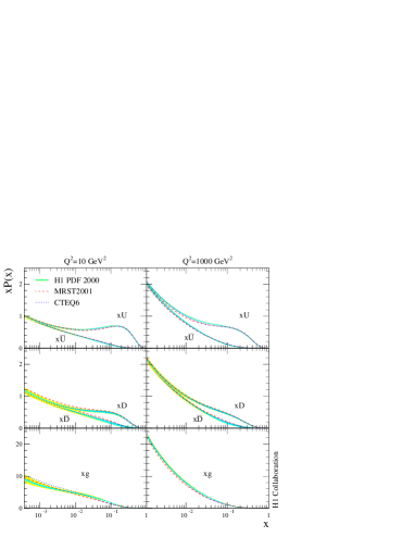
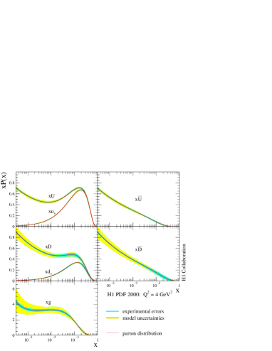
Figure 44: Determination of the sum of up, anti-up, down and anti-downquark distributions and of the gluon distribution in the proton based on the H1 neutral and charged current cross section data. Left: for $Q^{2}$ of 10 and 1000 GeV² compared with results from MRST and CTEQ; Right: the parton distributions with their experimental and model uncertainties as determined by H1 at the starting scale $Q^{2}_{0}=4$ GeV².

As is illustrated in Fig. 44 the H1 experiment [47] has determined all four quark distributions and the gluon distribution $xg$. The accuracy achieved so far by H1, for $x=0.01,0.4$ and $0.65$, is $1\%,\,3\%,7\%$ for the sum of up quark distributions and $2\%,\,10\%,30\%$ for the sum of down quark distributions, respectively. The extracted parton distributions are in reasonable agreement with the results obtained in global fits by the MRST [19] and CTEQ [18] collaborations. The H1 result is also consistent with the pdfs determined by the ZEUS Collaboration [46] which uses jet data to improve the accuracy for the gluon distribution and imports a $\overline{d}-\overline{u}$ asymmetry fit result from MRST. New data which are being taken (HERA II) will improve the accuracy of these determinations further. At the time this is written, the available data per experiment have been grown to roughly 150 pb^-1 for both $e^{+}p$ and $e^{-}p$ scattering, and more is still to come. These data will be particularly important to improve the accuracy at large $x$, which at HERA is related to high $Q^{2}$.

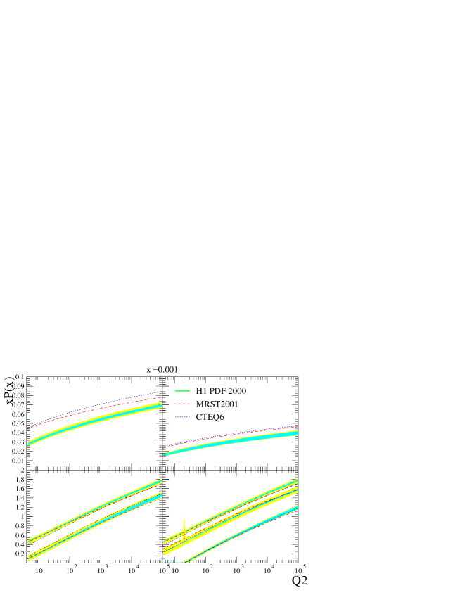
Figure 45: Parton distributions and their uncertainties as determined by H1 extrapolated to the region of the LHC, for $x=0.001$ near to the rapidity plateau. Top left: $u$ valence; top right: $d$ valence; bottom left: $\overline{u}$ and below $c$; bottom right, in decreasing order: $\overline{d}$, $s$, $b$. The results are compared with recent fits to global data by MRST and CTEQ. Note that at such small $x$ the valence quark distributions are very small. With increasing $Q^{2}$ the relative importance of the heavy quarks compared to the light quarks increases while the absolute difference of the quark distributions is observed to be rather independent of $Q^{2}$. The beauty contribution to the cross section thus becomes sizeable, amounting to about 5% for $pp\rightarrow HW$.

As is clear from the above equations, the NC and CC cross section data are sensitive directly to only these four quark distribution combinations. Disentangling the individual quark flavours (up, down, strange, charm and beauty) requires additional assumptions. While informations on the $c$ and $b$ densities are being obtained from measurements of $F_{2}^{c\overline{c}}$ and $F_{2}^{b\overline{b}}$ of improving accuracy, the determination of the strange quark density at HERA is less straightforward and may rest on $sW^{+}\rightarrow c$ and strange ($\Phi$) particle production [71]. The relative contributions from the heavy quarks become increasingly important with $Q^{2}$, as is illustrated in Fig. 45.

The larger $x$ domain is dominated by the valence quarks. At HERA the valence quark distributions are not directly determined but extracted from the differences $u_{v}=U-\overline{U}$ and $d_{v}=D-\overline{D}$. Note that this implies the assumption that sea and anti-quarks are equal which in non-perturbative QCD models may not hold. A perhaps more striking assumption is inherent in these fits and regards the sea quark asymmetries at low $x$ which is the main subject of the subsequent discussion.

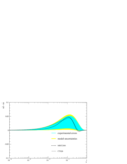
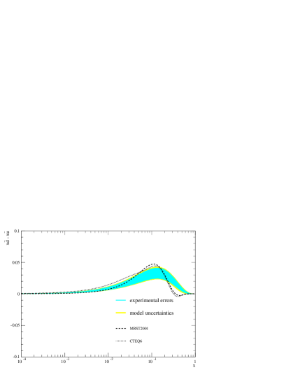
Figure 46: Determination of the difference $x(\overline{d}-\overline{u})$ in the H1 PDF 2000 fit to the H1 data (left) and the H1 and the BCDMS $\mu p$ and $\mu D$ data (right). The sea quark difference is enforced to tend to zero at low $x$. The global fit results of MRST and CTEQ include Drell Yan data which suggest a sea quark asymmetry at $x\sim 0.1$.

Fig. 46 shows the difference $x\overline{d}-x\overline{u}$ as determined in the H1 PDF 2000 fit based on the H1 data alone (left) and using in addition the BCDMS proton and deuteron data (right). One observes a trend of these fits to reproduce the asymmetry near $x\sim 0.1$ which in the MRST and CTEQ fits, shown in Fig. 46, is due to fitting the Drell Yan data from the E866/NuSea experiment [72]. While this enhancement is not very stable in the H1 fit [73] and not significant either, with the BCDMS data an asymmetry is observed which reflects the violation of the Gottfried sum rule.

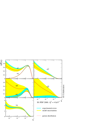
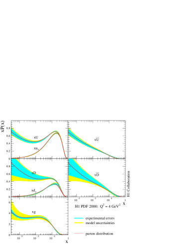
Figure 47: Determinations of the quark and gluon momentum distributions releasing the constraint $x\overline{d}=x\overline{u}$ at low $x$, from the H1 NC and CC data alone (left) and from the H1 $ep$ and the BCDMS $\mu p$ and $\mu D$ data (right). Since at low $x<0.01$ there is no further constraint than that given from $F_{2}$ the uncertainties of $\overline{U}$ and in particular of $\overline{D}$ become sizeable.

In the H1 fit [47] the parton distributions at the initial scale $Q^{2}=4$ GeV² are parameterised as $xP=A_{p}x^{B_{P}}(1-x)^{C_{P}}\cdot f_{P}(x)$. The function $f_{P}$ is a polynomial in $x$ which is determined by requiring “$\chi^{2}$ saturation” of the fits, i.e. starting from $f_{P}=1$ additional terms $D_{P}x$, $E_{P}x^{2}$ etc. are added and only considered if they cause a significant improvement in $\chi^{2}$, half integer powers were considered in [73]. The result for fitting the H1 data has been as follows: $f_{g}=(1+D_{g}x)$, $f_{U}=(1+D_{U}x+F_{U}x^{3})$, $f_{D}=(1+D_{D}x)$ and $f_{\overline{U}}=f_{\overline{D}}=1$. The parton distributions at low $x$ are thus parameterised as $xP\rightarrow A_{P}x^{B_{P}}$. The strange (charm) anti-quark distribution is coupled to the total amount of down (up) anti-quarks as $\overline{s}=f_{c}\overline{D}$ ($\overline{c}=f_{c}\overline{U}$). Two assumptions have been made on the behaviour of the quark and anti-quark distributions at low $x$. It has been assumed that quark and anti-quark distributions are equal and, moreover, that the sea is flavour symmetric. This implies that the slopes $B$ of all four quark distributions are set equal $B_{U}=B_{D}=B_{\overline{U}}=B_{\overline{D}}$. Moreover, the nomalisations of up and down quarks are the same, i.e. $A_{\overline{U}}(1-f_{c})=A_{\overline{D}}(1-f_{s})$, which ensures that $\overline{d}/\overline{u}\rightarrow 1$ as $x$ tends to zero. The consequence of this assumption is illustrated in Fig. 46. While the DIS data suggest some asymmetry at larger $x$, the up-down quark asymmetry is enforced to vanish at lower $x$. This results in a rather fake high accuracy in the determination of the four quark distributions at low $x$, despite the fact that at low $x$ there is only one combination of them measured, which is $F_{2}=x[4(U+\overline{U})+(D+\overline{D})]/9$. If one relaxes both the conditions on the slopes and normalisations, the fit to the H1 data decides to completely remove the down quark contributions as is seen in Fig. 47 (left plot).

In DIS the up and down quark asymmetry can be constrained using deuteron data because the nucleon structure function determines a different linear combination according to $F_{2}^{N}=5x(U+\overline{U}+D+\overline{D})/18+x(c+\overline{c}-s-\overline{s})/6$ with $N=(p+n)/2$. Unfortunately, there are only data at rather large $x$ available. The effect of including the BCDMS data on the low $x$ behaviour of the parton distributions is illustrated in Fig. 47 (right plot). It restores some amount of down quarks at low $x$ , the errors, however, in particular of the down quarks, are still very large. The result is a large sea quark asymmetry uncertainty, which is shown in Fig. 48. At HERA a proposal had been made [74] to operate the machine in electron-deuteron mode. Measuring the behaviour at low $x$ would not require high luminosity. Such data would constrain a possible sea quark asymmetry with very high accuracy, as is also shown in Fig. 48.

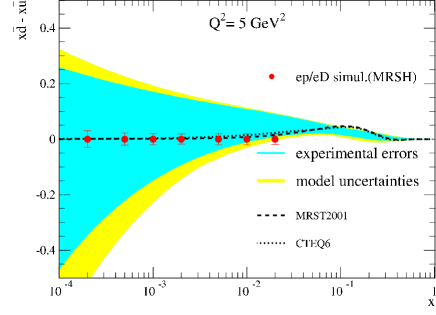
Figure 48: Simulation of the difference of sea quark distributions, here assumed to be zero, at low $x$ based on additional 20 pb^-1 of electron-deuteron data at HERA. The error band represents the uncertainty of the H1 NLO QCD fit to the H1 $ep$ and the BCDMS $\mu p$ and $\mu d$ data without the constraint $\overline{d}=\overline{u}$ at low $x$. The dashed curves represent calculations using recent global fits by MRST and by CTEQ.

Deuterons at HERA would require a new source and modest modifications to the preaccelerators. The H1 apparatus could be used in its standard mode with a forward proton detector added to take data at half the beam energy. Tagging the spectator protons with high accuracy at HERA, for the first time in DIS, one could reconstruct the electron-neutron scattering kinematics essentially free of nuclear corrections [74]. Since the forward scattering amplitude is related to diffraction one would also be able to constrain shadowing to the per cent level [80]. The low $x$ measurements would require small luminosity amounts, of less than 50 pb^-1. Long awaited constraints of the $d/u$ ratio at large $x$ and $Q^{2}$ would require extended running, as would CC data. Besides determining the parton distributions better, the measurement of the singlet $F_{2}^{N}$ structure function would give important constraints on the evolution and theory at low $x$ [81]. It would also result in an estimated factor of two improvement on the measurement of $\alpha_{s}$ at HERA [82]. For the development of QCD, of low $x$ physics in particular, but as well for understanding physics at the LHC and also for superhigh energy neutrino astrophysics, HERA $eD$ data remain to be important.

3.7 Impact of future HERA data on the determination of proton PDFs using the ZEUS NLO QCD fit

3.7.1 PDF fits to HERA data

Recently, the ZEUS Collaboration have performed a combined NLO QCD fit to inclusive neutral and charged current DIS data [54, 56, 58, 55, 57, 59] as well as high precision jet data in DIS [83] and $\gamma p$ scattering [84]. This is called the ZEUS-JETS PDF fit [46]. The use of only HERA data eliminates the uncertainties from heavy-target corrections and removes the need for isospin symmetry assumptions. It also avoids the difficulties that can sometimes arise from combining data-sets from several different experiments, thereby allowing a rigorous statistical treatment of the PDF uncertainties. Furthermore, PDF uncertainties from current global fits are, in general, limited by (irreducible) experimental systematics. In contrast, those from fits to HERA data alone, are largely limited by the statistical precision of existing measurements. Therefore, the impact of future data from HERA is likely to be most significant in fits to only HERA data.

		HERA-I	HERA-II
data sample	kinematic coverage	$\mathcal{L}$ (${\rm pb}^{-1}$)	$\mathcal{L}$ (${\rm pb}^{-1}$)
			(assumed)
96-97 NC $e^{+}p$ [54]	$2.7<Q^{2}<30000$ ${\rm GeV}^{2}$; $6.3\cdot 10^{-5}<x<0.65$	30	30
94-97 CC $e^{+}p$ [55]	$280<Q^{2}<17000$ ${\rm GeV}^{2}$; $6.3\cdot 10^{-5}<x<0.65$	48	48
98-99 NC $e^{-}p$ [56]	$200<Q^{2}<30000$ ${\rm GeV}^{2}$; $0.005<x<0.65$	16	350
98-99 CC $e^{-}p$ [57]	$280<Q^{2}<17000$ ${\rm GeV}^{2}$; $0.015<x<0.42$	16	350
99-00 NC $e^{+}p$ [58]	$200<Q^{2}<30000$ ${\rm GeV}^{2}$; $0.005<x<0.65$	63	350
99-00 CC $e^{+}p$ [59]	$280<Q^{2}<17000$ ${\rm GeV}^{2}$; $0.008<x<0.42$	61	350
96-97 inc. DIS jets [83]	$125<Q^{2}<30000$ ${\rm GeV}^{2}$; $E_{\rm T}^{Breit}>8$ GeV	37	500
96-97 dijets in $\gamma p$ [84]	$Q^{2}\lesssim 1$ ${\rm GeV}^{2}$; $E_{\rm T}^{jet1,2}>14,11$ ${\rm GeV}$	37	500
optimised jets [85]	$Q^{2}\lesssim 1$ ${\rm GeV}^{2}$; $E_{\rm T}^{jet1,2}>20,15$ ${\rm GeV}$	-	500

Table 11: The data-sets included in the ZEUS-JETS and HERA-II projected PDF fits. The first column lists the type of data and the second gives the kinematic coverage. The third column gives the integrated luminosities of the HERA-I measurements included in the ZEUS-JETS fit. The fourth column gives the luminosities assumed in the HERA-II projection. Note that the 96-97 NC and the 94-97 CC measurements have not had their luminosity scaled for the HERA-II projection.

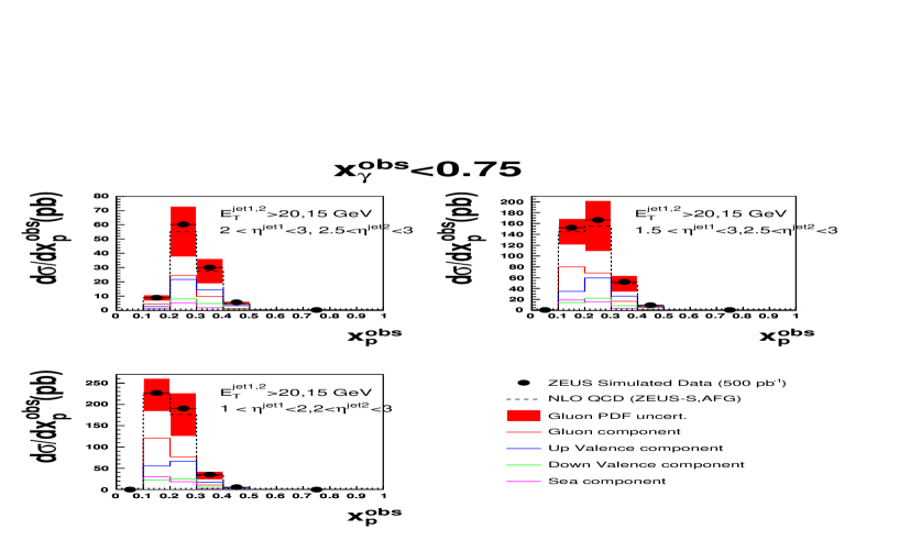
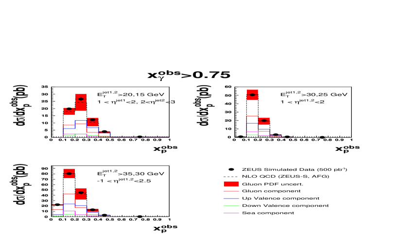
Figure 49: The optimised jet cross sections included in the HERA-II projected fit. The solid points show the simulated data generated using the NLO QCD programme of Frixione-Ridolfi, using the CTEQ5M1 proton and the AFG photon PDFs. The error bars show the statistical uncertainties, which correspond to $500$ ${\rm pb}^{-1}$ of HERA data. Systematic uncertainties have been neglected. The dashed line shows the NLO QCD prediction using the ZEUS-S proton and AFG photon PDFs. The shaded band shows the contribution to the cross section uncertainty arising from the uncertainty in the gluon distribution in the proton.

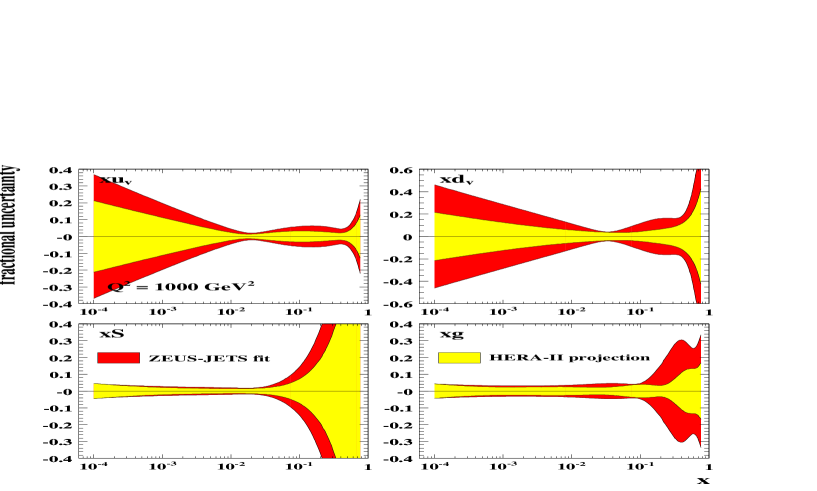
Figure 50: The fractional PDF uncertainties, as a function of $x$, for the $u$-valence, $d$-valence, sea-quark and gluon distributions at $Q^{2}=$ 1000 ${\rm GeV}^{2}$. The red shaded bands show the results of the ZEUS-JETS fit and the yellow shaded bands show the results of the HERA-II projected fit.

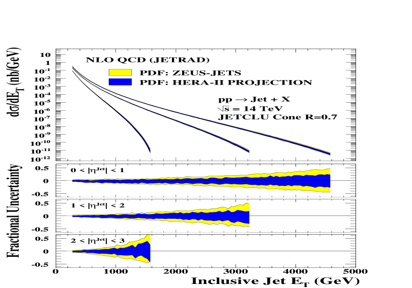
Figure 51: NLO QCD inclusive jet cross section predictions at $\sqrt{s}$=14 TeV in three regions of pseudo-rapidity. The yellow and blue bands show the PDF uncertainties from the ZEUS-JETS and HERA-II projected fits, respectively.

3.7.2 The ZEUS NLO QCD fit

The ZEUS-JETS PDF fit has been used as the basis for all results shown in this contribution. The most important details of the fit are summarised here. A full description may be found elsewhere [46]. The fit includes the full set of ZEUS inclusive neutral and charged current $e^{\pm}p$ data from HERA-I (1994-2000), as well as two sets of high precision jet data in $e^{+}p$ DIS ($Q^{2}>>1$ ${\rm GeV}^{2}$) and $\gamma p$ ($Q^{2}\sim 0$) scattering. The inclusive data used in the fit, span the kinematic range $6.3\times 10^{-5}<x<0.65$ and $2.7<Q^{2}<30000$ ${\rm GeV}^{2}$.

The PDFs are obtained by solving the NLO DGLAP equations within the $\overline{{\rm MS}}$ scheme. These equations yield the PDFs at all values of $Q^{2}$ provided they are input as functions of $x$ at some starting scale $Q_{0}^{2}$. The resulting PDFs are convoluted with coefficient functions to give predictions for structure functions and, hence, cross sections. In the ZEUS fit, the $xu_{v}(x)$ ($u$-valence), $xd_{v}(x)$ ($d$-valence), $xS(x)$ (total sea-quark), $xg(x)$ (gluon) and $x(\bar{d}(x)-\bar{u}(x))$ PDFs are parameterised at a starting scale of $Q_{0}^{2}=7$ ${\rm GeV}^{2}$ by the form,

$$xf(x)=p_{1}x^{p_{2}}(1-x)^{p_{3}}P(x),$$ (16)

where $P(x)=(1+p_{4}x)$. No advantage in the $\chi^{2}$ results from using more complex polynomial forms. The normalisation parameters, $p_{1}(u_{v})$ and $p_{1}(d_{v})$, are constrained by quark number sum rules while $p_{1}(g)$ is constrained by the momentum sum rule. Since there is no information to constrain any difference in the low-$x$ behaviour of the $u$- and $d$-valence quarks, $p_{2}(u_{v})$ has been set equal to $p_{2}(d_{v})$. The data from HERA are currently less precise than the fixed target data in the high-$x$ regime. Therefore, the high-$x$ sea and gluon distributions are not well constrained in current fits to HERA data alone. To account for this, the sea shape has been restricted by setting $p_{4}(S)=0$. The high-$x$ gluon shape is constrained by the inclusion of HERA jet data. In fits to only HERA data, there is no information on the shape of $\bar{d}-\bar{u}$. Therefore, this distribution has its shape fixed consistent with Drell-Yan data and its normalisation set consistent with the size of the Gottfried sum rule violation. A suppression of the strange sea with respect to the non-strange sea of a factor of 2 at $Q_{0}^{2}$ is also imposed, consistent with neutrino induced dimuon data from CCFR. The value of the strong coupling has been fixed to $\alpha_{s}(M_{\rm Z})=0.1180$. After all constraints, the ZEUS-JETS fit has 11 free parameters. Heavy quarks were treated in the variable flavour number scheme of Thorne & Roberts [50]. Full account was taken of correlated experimental systematic uncertainties, using the Offset Method [45, 49].

The results of two separate studies are presented. The first study provides an estimate of how well the PDF uncertainties may be known by the end of HERA-II, within the currently planned running scenario, while the second study investigates the impact of a future HERA measurement of ${F_{L}}$ on the gluon distribution. All results presented, are based on the recent ZEUS-JETS PDF analysis [46].

3.7.3 PDF uncertainty estimates for the end of HERA running

The data from HERA-I are already very precise and cover a wide kinematic region. However, HERA-II is now running efficiently and is expected to provide a substantial increase in luminosity. Current estimates suggest that, by the end of HERA running (in mid-2007), an integrated luminosity of $700$ ${\rm pb}^{-1}$ should be achievable. This will allow more precise measurements of cross sections that are curently statistically limited: in particular, the high-$Q^{2}$ NC and CC data, as well as high-$Q^{2}$ and/or high-$E_{\rm T}$ jet data. In addition to the simple increase in luminosity, recent studies [85] have shown that future jet cross section measurements, in kinematic regions optimised for sensitivity to PDFs, should have a significant impact on the gluon uncertainties. In this contribution, the effect on the PDF uncertainties, of both the higher precision expected from HERA-II and the possibility of optimised jet cross section measurements, has been estimated in a new QCD fit. This fit will be referred to as the “HERA-II projection”.

In the HERA-II projected fit, the statistical uncertainties on the currently available HERA-I data have been reduced. For the high-$Q^{2}$ inclusive data, a total integrated luminosity of $700$ ${\rm pb}^{-1}$ was assumed, equally divided between $e^{+}$ and $e^{-}$. For the jet data, an integrated luminosity of $500$ ${\rm pb}^{-1}$ was assumed. The central values and systematic uncertainties were taken from the published data in each case. In addition to the assumed increase in precision of the measurements, a set of optimised jet cross sections were also included, for forward dijets in $\gamma p$ collisions, as defined in a recent study [85]. Since no real data are yet available, simulated points were generated using the NLO QCD program of Frixione-Ridolfi [86], using the CTEQ5M1 [18] proton and AFG [87] photon PDFs. The statistical uncertainties were taken to correspond to $500$ ${\rm pb}^{-1}$. For this study, systematic uncertainties on the optimised jet cross sections were ignored. The simulated optimised jet cross section points, compared to the predictions of NLO QCD using the ZEUS-S proton PDF [45], are shown in Fig. 49.

Table 11 lists the data-sets included in the ZEUS-JETS and HERA-II projected fits. The luminosities of the (real) HERA-I measurements and those assumed for the HERA-II projection are also given.

The results are summarised in Fig. 50, which shows the fractional PDF uncertainties, for the $u$- and $d$-valence, sea-quark and gluon distributions, at $Q^{2}=1000$ ${\rm GeV}^{2}$. The yellow bands show the results of the ZEUS-JETS fit while the red bands show those for the HERA-II projection. Note that the same general features are observed for all values of $Q^{2}$. In fits to only HERA data, the information on the valence quarks comes from the high-$Q^{2}$ NC and CC cross sections. The increased statistical precision of the high-$Q^{2}$ data, as assumed in the HERA-II projected fit, gives a significant improvement in the valence uncertainties over the whole range of $x$. For the sea quarks, a significant improvement in the uncertainties at high-$x$ is also observed. In contrast, the low-$x$ uncertainties are not visibly reduced. This is due to the fact that the data constraining the low-$x$ region tends to be at lower-$Q^{2}$, which are already systematically limited. This is also the reason why the low-$x$ gluon uncertainties are not significantly reduced. However, the mid-to-high-$x$ gluon, which is constrained by the jet data, is much improved in the HERA-II projected fit. Note that about half of the observed reduction in the gluon uncertainties is due to the inclusion of the simulated optimised jet cross sections.

Inclusive jet cross sections at the LHC

The improvement to the high-$x$ partons, observed in the HERA-II projection compared to the ZEUS-JETS fit, will be particularly relevant for high-scale physics at the LHC. This is illustrated in Fig. 51, which shows NLO QCD predictions from the JETRAD [88] programme for inclusive jet production at $\sqrt{s}=14$ TeV. The results are shown for both the ZEUS-JETS and the HERA-II projected PDFs. The uncertainties on the cross sections, resulting from the PDFs, have been calculated using the LHAPDF interface [89]. For the ZEUS-JETS PDF, the uncertainty reaches $\sim 50\%$ at central pseudo-rapidities, for the highest jet transverse energies shown. The prediction using the HERA-II projected PDF shows a marked improvement at high jet tranverse energy.

3.7.4 Impact of a future HERA measurement of $F_{L}$ on the gluon PDF

The longitudinal structure function, ${F_{L}}$, is directly related to the gluon density in the proton. In principle, ${F}_{L}$ can be extracted by measuring the NC DIS cross section at fixed $x$ and $Q^{2}$, for different values of $y$ (see Eqn. 4). A precision measurement could be achieved by varying the centre-of-mass energy, since $s=Q^{2}/xy\approx 4E_{e}E_{p}$, where $E_{e}$ and $E_{p}$ are the electron and proton beam energies, respectively. Studies [68] (Sec. 3.5) have shown that this would be most efficiently achieved by changing the proton beam energy. However, such a measurement has not yet been performed at HERA.

There are several reasons why a measurement of ${F_{L}}$ at low-$x$ could be important. The gluon density is not well known at low-$x$ and so different PDF parameterisations can give quite different predictions for ${F_{L}}$ at low-$x$. Therefore, a precise measurement of the longitudinal sturcture function could both pin down the gluon PDF and reduce its uncertainties. Furthermore, predictions of ${F_{L}}$ also depend upon the nature of the underlying theory (e.g. order in QCD, resummed calculation etc). Therefore, a measurement of ${F_{L}}$ could also help to discriminate between different theoretical models.

Impact on the gluon PDF uncertainties

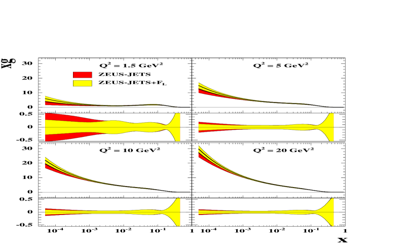
Figure 52: The gluon PDFs, showing also the fractional uncertainty, for fits with and without inclusion of the simulated ${F_{L}}$ data, for $Q^{2}=$ 1.5, 5, 10 and 20 ${\rm GeV}^{2}$. The red shaded bands show the results of the ZEUS-JETS fit and the yellow shaded band show the results of the ZEUS-JETS+${F_{L}}$ fit.

The impact of a possible future HERA measurement of ${F_{L}}$ on the gluon PDF uncertainties has been investigated, using a set of simulated ${F_{L}}$ data-points [68]. (see Sec. 3.5). The simulation was performed using the GRV94 [90] proton PDF for the central values, and assuming $E_{e}=27.6$ GeV and $E_{p}=920,575,465$ and $400$ GeV, with luminosities of 10, 5, 3 and 2 ${\rm pb}^{-1}$, respectively. Assuming that the luminosity scales simply as $E_{p}^{2}$, this scenario would nominally cost $35$ ${\rm pb}^{-1}$ of luminosity under standard HERA conditions. However, this estimate takes no account of time taken for optimisation of the machine with each change in $E_{p}$, which could be considerable. The systematic uncertainties on the simulated data-points were calculated assuming a $\sim 2\%$ precision on the inclusive NC cross section measurement. A more comprehensive description of the simulated data is given in contribution for this proceedings, see Sec. 3.5.

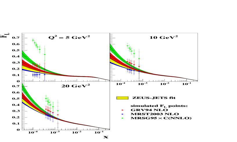
Figure 53: The distribution of the longitudinal structure function ${F_{L}}$ at $Q^{2}=$5, 10 and 20 ${\rm GeV}^{2}$. The blue, red and green points show the simulated ${F_{L}}$ data-points, respectively labelled maximum, middle and minimum in Table 12. The blue, red and green shaded bands show the NLO QCD predictions, in the case where the data-points of the corresponding colour have been included in the fit. For comparison, the yellow shaded band shows the prediction of the ZEUS-JETS fit.

The simulated data were included in the ZEUS-JETS fit. Figure 52 shows the gluon distribution and fractional uncertainties for fits with and without inclusion of the simulated ${F_{L}}$ data. The results indicate that the gluon uncertainties are reduced at low-$x$, but the improvement is only significant at relatively low $Q^{2}\lesssim 20$ ${\rm GeV}^{2}$.

Discrimination between theoretical models

In order to assess whether a HERA measurement of ${F_{L}}$ could discriminate between theoretical models, two more sets of ${F_{L}}$ data-points have been simulated [91], using different theoretical assumptions. The first of the two sets was generated using the MRSG95 [92] proton PDF, which has a large gluon density. The PDFs were then convoluted with the NNLO order coefficient functions, which are large and positive. This gives the “maximum” set of ${F_{L}}$ data-points. In contrast, the second set has been generated using the MRST2003 [93] proton PDF, which has a negative gluon at low-$x$ and low-$Q^{2}$, thus providing a “minimum” set of ${F_{L}}$ data. The original set of ${F_{L}}$ points described in the previous subsection lies between these two extremes. The details of all three sets are summarised in Tab. 12.

Figure 53 shows the results of including, individually, each set of simulated ${F_{L}}$ data into the ZEUS NLO QCD fit. The results show that the NLO fit is relatively stable to the inclusion of the extreme sets of data. This indicates that a measurement of ${F_{L}}$ could discriminate between certain theoretical models. However, it should be noted that the maximum and minimum models studied here were chosen specifically to give the widest possible variation in ${F_{L}}$. There are many other alternatives that would lie between these extremes and the ability of an ${F_{L}}$ measurement to discriminate between them would depend both on the experimental precision of the measurement itself, as well as the theoretical uncertainties on the models being tested.

	PDF	QCD order of coefficient functions
Maximum ${F_{L}}$	MRSG95	NNLO
Middle ${F_{L}}$	GRV94	NLO
Minimum ${F_{L}}$	MRST2003	NLO

Table 12: Summary of the PDFs used to generate the simulated ${F_{L}}$ data-points. The extreme maximum $F_{L}$ points were generated using the MRSG95 PDF, and convoluted with NNLO coefficient functions. The middle points were generated using the GRV94 PDF, and the extreme minimum points were generated using the MRST2003 PDF, which has a negative gluon at low-$x$.

3.8 A Method to Include Final State Cross-sections Measured in Proton-Proton Collisions to Global NLO QCD Analysis

The Large Hadron Collider (LHC), currently under construction at CERN, will collide protons on protons with an energy of $7$ TeV. Together with its high collision rate the high available centre-of-mass energy will make it possible to test new interactions at very short distances that might be revealed in the production cross-sections of Standard Model (SM) particles at very high transverse momentum ($P_{T}$) as deviation from the SM theory.

The sensitivity to new physics crucially depends on experimental uncertainties in the measurements and on theoretical uncertainties in the SM predictions. It is therefore important to work out a strategy to minimize both the experimental and theoretical uncertainties from LHC data. For instance, one could use single inclusive jet or Drell-Yan cross-sections at low $P_{T}$ to constrain the PDF uncertainties at high $P_{T}$. Typical residual renormalisation and factorisation scale uncertainties in next-to-leading order (NLO) calculations for single inclusive jet-cross-section are about $5-10\%$ and should hopefully be reduced as NNLO calculations become available. The impact of PDF uncertainties on the other hand can be substantially larger in some regions, especially at large $P_{T}$, and for example at $P_{T}=2000$ GeV dominate the overall uncertainty of $20\%$. If a suitable combination of data measured at the Tevatron and LHC can be included in global NLO QCD analyses, the PDF uncertainties can be constrained.

The aim of this contribution is to propose a method for consistently including final-state observables in global QCD analyses.

For inclusive data like the proton structure function $F_{2}$ in deep-inelastic scattering (DIS) the perturbative coefficients are known analytically. During the fit the cross-section can therefore be quickly calculated from the strong coupling ($\alpha_{\rm s}$) and the PDFs and can be compared to the measurements. However, final state observables, where detector acceptances or jet algorithms are involved in the definition of the perturbative coefficients (called “weights” in the following), have to be calculated using NLO Monte Carlo programs. Typically such programs need about one day of CPU time to calculate accurately the cross-section. It is therefore necessary to find a way to calculate the perturbative coefficients with high precision in a long run and to include $\alpha_{\rm s}$ and the PDFs “a posteriori”.

To solve this problem many methods have been proposed in the past [94, 95, 96, 41, 97, 46]. In principle the highest efficiencies can be obtained by taking moments with respect to Bjorken-$x$ [94, 95], because this converts convolutions into multiplications. This can have notable advantages with respect to memory consumption, especially in cases with two incoming hadrons. On the other hand, there are complications such as the need for PDFs in moment space and the associated inverse Mellin transforms.

Methods in $x$-space have traditionally been somewhat less efficient, both in terms of speed (in the ‘a posteriori’ steps — not a major issue here) and in terms of memory consumption. They are, however, somewhat more transparent since they provide direct information on the $x$ values of relevance. Furthermore they can be used with any PDF. The use of $x$-space methods can be further improved by using methods developed originally for PDF evolution [98, 99].

3.8.1 PDF-independent representation of cross-sections

Representing the PDF on a grid

We make the assumption that PDFs can be accurately represented by storing their values on a two-dimensional grid of points and using $n^{\mathrm{th}}$-order interpolations between those points. Instead of using the parton momentum fraction $x$ and the factorisation scale $Q^{2}$, we use a variable transformation that provides good coverage of the full $x$ and $Q^{2}$ range with uniformly spaced grid points:

$$y(x)=\ln\frac{1}{x}\;\;\;{\rm and}\;\;\;\tau(Q^{2})=\ln\ln\frac{Q^{2}}{\Lambda^{2}}.$$ (17)

The parameter $\Lambda$ is to be chosen of the order of $\Lambda_{\mathrm{QCD}}$, but not necessarily identical. The PDF $q(x,Q^{2})$ is then represented by its values $q_{i_{y},i_{\tau}}$ at the 2-dimensional grid point $(i_{y}\,\delta y,i_{\tau}\,\delta\tau)$, where $\delta y$ and $\delta\tau$ denote the grid spacings, and obtained elsewhere by interpolation:

$$q(x,Q^{2})=\sum_{i=0}^{n}\sum_{\iota=0}^{n^{\prime}}q_{k+i,\kappa+\iota}\,\,I_{i}^{(n)}\left(\frac{y(x)}{\delta y}-k\right)\,I_{\iota}^{(n^{\prime})}\left(\frac{\tau(Q^{2})}{\delta\tau}-\kappa\right),$$ (18)

where $n$, $n^{\prime}$ are the interpolation orders. The interpolation function $I_{i}^{(n)}(u)$ is 1 for $u=i$ and otherwise is given by:

$$I_{i}^{(n)}(u)=\frac{(-1)^{n-i}}{i!(n-i)!}\frac{u(u-1)\ldots(u-n)}{u-i}\,.$$ (19)

Defining $\mathrm{int}(u)$ to be the largest integer such that $\mathrm{int}(u)\leq u$, $k$ and $\kappa$ are defined as:

$$k(x)= \mathrm{int}\left(\frac{y(x)}{\delta y}-\frac{n-1}{2}\right), \kappa(x)=\mathrm{int}\left(\frac{\tau(Q^{2})}{\delta\tau}-\frac{n^{\prime}-1}{2}\right).$$ (20)

Given finite grids whose vertex indices range from $0\ldots N_{y}-1$ for the $y$ grid and $0\ldots N_{\tau}-1$ for the $\tau$ grid, one should additionally require that eq. (18) only uses available grid points. This can be achieved by remapping $k\to\max(0,\min(N_{y}-1-n,k))$ and $\kappa\to\max(0,\min(N_{\tau}-1-n^{\prime},\kappa))$.

Representing the final state cross-section weights on a grid (DIS case)

Suppose that we have an NLO Monte Carlo program that produces events $m=1\dots N$. Each event $m$ has an $x$ value, $x_{m}$, a $Q^{2}$ value, $Q^{2}_{m}$, as well as a weight, $w_{m}$, and a corresponding order in $\alpha_{\rm s}$, $p_{m}$. Normally one would obtain the final result $W$ of the Monte Carlo integration from:

$$W=\sum_{m=1}^{N}\,w_{m}\,\left(\frac{\alpha_{s}(Q_{m}^{2})}{2\pi}\right)^{p_{m}}\,q(x_{m},Q^{2}_{m}).$$ (21)

Instead one introduces a weight grid $W_{i_{y},i_{\tau}}^{(p)}$ and then for each event updates a portion of the grid with:
$i=0\dots n,\;\iota=0\dots n^{\prime}:$

$$W_{k+i,\kappa+\iota}^{(p_{m})}\to W_{k+i,\kappa+\iota}^{(p_{m})}+w_{m}\,I_{i}^{(n)}\left(\frac{y(x_{m})}{\delta y}-k\right)I_{\iota}^{(n^{\prime})}\left(\frac{\tau(Q^{2}_{m})}{\delta\tau}-\kappa\right),$$ (22)

$$\;\;\;{\rm where}\;\;\;k\equiv k(x_{m}),\;\kappa\equiv\kappa(Q^{2}_{m}).$$

The final result for $W$, for an arbitrary PDF, can then be obtained subsequent to the Monte Carlo run:

$$W=\sum_{p}\sum_{i_{y}}\sum_{i_{\tau}}W_{i_{y},i_{\tau}}^{(p)}\,\left(\frac{\alpha_{s}\left({Q^{2}}^{(i_{\tau})}\right)}{2\pi}\right)^{p}q\!\left(x^{(i_{y})},{Q^{2}}^{(i_{\tau})}\right)\,,$$ (23)

where the sums index with $i_{y}$ and $i_{\tau}$ run over the number of grid points and we have have explicitly introduced $x^{(i_{y})}$ and ${Q^{2}}^{(i_{\tau})}$ such that:

$$y(x^{(i_{y})})=i_{y}\,\delta y\quad{\rm and}\quad\tau\left({Q^{2}}^{(i_{\tau})}\right)=i_{\tau}\,\delta\tau.$$ (24)

Including renormalisation and factorisation scale dependence

If one has the weight matrix $W_{i_{y},i_{\tau}}^{(p)}$ determined separately order by order in $\alpha_{\rm s}$, it is straightforward to vary the renormalisation $\mu_{R}$ and factorisation $\mu_{F}$ scales a posteriori (we assume that they were kept equal in the original calculation).

It is helpful to introduce some notation relating to the DGLAP evolution equation:

$$\frac{dq(x,Q^{2})}{d\ln Q^{2}}=\frac{\alpha_{s}(Q^{2})}{2\pi}(P_{0}\otimes q)(x,Q^{2})+\left(\frac{\alpha_{s}(Q^{2})}{2\pi}\right)^{2}(P_{1}\otimes q)(x,Q^{2})+\ldots,$$ (25)

where the $P_{0}$ and $P_{1}$ are the LO and NLO matrices of DGLAP splitting functions that operate on vectors (in flavour space) $q$ of PDFs. Let us now restrict our attention to the NLO case where we have just two values of $p$, $p_{\mathrm{LO}}$ and $p_{\mathrm{NLO}}$. Introducing $\xi_{R}$ and $\xi_{F}$ corresponding to the factors by which one varies $\mu_{R}$ and $\mu_{F}$ respectively, for arbitrary $\xi_{R}$ and $\xi_{F}$ we may then write:

$$W(\xi_{R},\xi_{F})=\sum_{i_{y}}\sum_{i_{\tau}}\left(\frac{\alpha_{s}\left(\xi_{R}^{2}{Q^{2}}^{(i_{\tau})}\right)\,}{2\pi}\right)^{p_{\mathrm{LO}}}W_{i_{y},i_{\tau}}^{(p_{\mathrm{LO}})}q\!\left(x^{(i_{y})},\xi_{F}^{2}{Q^{2}}^{(i_{\tau})}\right)+$$

$$\left(\frac{\alpha_{s}\left(\xi_{R}^{2}{Q^{2}}^{(i_{\tau})}\right)\,}{2\pi}\right)^{p_{\mathrm{NLO}}}\left[\left(W_{i_{y},i_{\tau}}^{(p_{\mathrm{NLO}})}+2\pi\beta_{0}p_{\mathrm{LO}}\ln\xi_{R}^{2}\,W_{i_{y},i_{\tau}}^{(p_{\mathrm{LO}})}\right)q\!\left(x^{(i_{y})},\xi_{F}^{2}{Q^{2}}^{(i_{\tau})}\right)\right.$$ (26)

$$\left.-\ln\xi_{F}^{2}\,W_{i_{y},i_{\tau}}^{(p_{\mathrm{LO}})}(P_{0}\otimes q)\!\left(x^{(i_{y})},\xi_{F}^{2}{Q^{2}}^{(i_{\tau})}\right)\right]\,,$$

where $\beta_{0}=(11N_{c}-2n_{f})/(12\pi)$ and $N_{c}$ ($n_{f}$) is the number of colours (flavours). Though this formula is given for $x$-space based approach, a similar formula applies for moment-space approaches. Furthermore it is straightforward to extend it to higher perturbative orders.

Representing the weights in the case of two incoming hadrons

In hadron-hadron scattering one can use analogous procedures with one more dimension. Besides $Q^{2}$, the weight grid depends on the momentum fraction of the first ($x_{1}$) and second ($x_{2}$) hadron.

In the case of jet production in proton-proton collisions the weights generated by the Monte Carlo program as well as the PDFs can be organised in seven possible initial state combinations of partons:

$$\mathrm{gg}:\;\;F^{(0)}(x_{1},x_{2};Q^{2}) = G_{1}(x_{1})G_{2}(x_{2})$$ (27)

$$\mathrm{qg}:\;\;F^{(1)}(x_{1},x_{2};Q^{2}) = \left(Q_{1}(x_{1})+\overline{Q}_{1}(x_{1})\right)G_{2}(x_{2})$$ (28)

$$\mathrm{gq}:\;\;F^{(2)}(x_{1},x_{2};Q^{2}) = G_{1}(x_{1})\left(Q_{2}(x_{2})+\overline{Q}_{2}(x_{2})\right)$$ (29)

$$\mathrm{qr}:\;\;F^{(3)}(x_{1},x_{2};Q^{2}) = Q_{1}(x_{1})Q_{2}(x_{2})+\overline{Q}_{1}(x_{1})\overline{Q}_{2}(x_{2})-D(x_{1},x_{2})$$ (30)

$$\mathrm{qq}:\;\;F^{(4)}(x_{1},x_{2};Q^{2}) = D(x_{1},x_{2})$$ (31)

$$\mathrm{q\bar{q}}:\;\;F^{(5)}(x_{1},x_{2};Q^{2}) = \overline{D}(x_{1},x_{2})$$ (32)

$$\mathrm{q\bar{r}}:\;\;F^{(6)}(x_{1},x_{2};Q^{2}) = Q_{1}(x_{1})\overline{Q}_{2}(x_{2})+\overline{Q}_{1}(x_{1})Q_{2}(x_{2})-\overline{D}(x_{1},x_{2}),$$ (33)

where $g$ denotes gluons, $q$ quarks and $r$ quarks of different flavour $q\neq r$ and we have used the generalized PDFs defined as:

$$G_{H}(x)=f_{0/H}(x,Q^{2}), Q_{H}(x)=\sum_{i=1}^{6}f_{i/H}(x,Q^{2}),\;\;\overline{Q}_{H}(x)=\sum_{i=-6}^{-1}f_{i/H}(x,Q^{2}),$$

$$D(x_{1},x_{2}) = \mathop{\sum_{i=-6}^{6}}_{i\neq 0}f_{i/H_{1}}(x_{1},Q^{2})f_{i/H_{2}}(x_{2},Q^{2}),$$ (34)

$$\overline{D}(x_{1},x_{2},\mu^{2}_{F}) = \mathop{\sum_{i=-6}^{6}}_{i\neq 0}f_{i/H_{1}}(x_{1},Q^{2})f_{-i/H_{2}}(x_{2},Q^{2}),\;\;$$

where $f_{i/H}$ is the PDF of flavour $i=-6\dots 6$ for hadron $H$ and $H_{1}$ ($H_{2}$) denotes the first or second hadron.

The analogue of eq. 23 is then given by:

$$W=\sum_{p}\sum_{l=0}^{6}\sum_{i_{y_{1}}}\sum_{i_{y_{2}}}\sum_{i_{\tau}}W_{i_{y_{1}},i_{y_{2}},i_{\tau}}^{(p)(l)}\,\left(\frac{\alpha_{s}\left({Q^{2}}^{(i_{\tau})}\right)}{2\pi}\right)^{p}F^{(l)}\left(x_{1}^{(i_{y_{1}})},x_{2}^{(i_{y_{1}})},{Q^{2}}^{(i_{\tau})}\right).$$ (35)

Including scale depedence in the case of two incoming hadrons

It is again possible to choose arbitrary renormalisation and factorisation scales, specifically for NLO accuracy:

$$W(\xi_{R},\xi_{F})=\sum_{l=0}^{6}\sum_{i_{y_{1}}}\sum_{i_{y_{2}}}\sum_{i_{\tau}}\left(\frac{\alpha_{s}\left(\xi_{R}^{2}{Q^{2}}^{(i_{\tau})}\right)\,}{2\pi}\right)^{p_{\mathrm{LO}}}W_{i_{y_{1}},i_{y_{2}},i_{\tau}}^{(p_{\mathrm{LO}})(l)}F^{(l)}\left(x_{1}^{(i_{y_{1}})},x_{2}^{(i_{y_{1}})},\xi_{F}^{2}{Q^{2}}^{(i_{\tau})}\right)+$$

$$\left(\frac{\alpha_{s}\left(\xi_{R}^{2}{Q^{2}}^{(i_{\tau})}\right)\,}{2\pi}\right)^{p_{\mathrm{NLO}}}\left[\left(W_{i_{y_{1}},i_{y_{2}},i_{\tau}}^{(p_{\mathrm{NLO}})(l)}+2\pi\beta_{0}p_{\mathrm{LO}}\ln\xi_{R}^{2}\,W_{i_{y_{1}},i_{y_{2}},i_{\tau}}^{(p_{\mathrm{LO}})(l)}\right)F^{(l)}\left(x_{1}^{(i_{y_{1}})},x_{2}^{(i_{y_{1}})},\xi_{F}^{2}{Q^{2}}^{(i_{\tau})}\right)\right.$$ (36)

$$\left.-\ln\xi_{F}^{2}\,W_{i_{y_{1}},i_{y_{2}},i_{\tau}}^{(p_{\mathrm{LO}})(l)}\left(F^{(l)}_{q_{1}\to P_{0}\otimes q_{1}}\left(x_{1}^{(i_{y_{1}})},x_{2}^{(i_{y_{1}})},\xi_{F}^{2}{Q^{2}}^{(i_{\tau})}\right)+F^{(l)}_{q_{2}\to P_{0}\otimes q_{2}}\left(x_{1}^{(i_{y_{1}})},x_{2}^{(i_{y_{1}})},\xi_{F}^{2}{Q^{2}}^{(i_{\tau})}\right)\right)\right]\,,$$

where $F^{(l)}_{q_{1}\to P_{0}\otimes q_{1}}$ is calculated as $F^{(l)}$, but with $q_{1}$ replaced wtih $P_{0}\otimes q_{1}$, and analogously for $F^{(l)}_{q_{2}\to P_{0}\otimes q_{2}}$.

3.8.2 Technical implementation

To test the scheme discussed above we use the NLO Monte Carlo program NLOJET++ [100] and the CTEQ6 PDFs [18]. The grid $W_{i_{y_{1}},i_{y_{2}},i_{\tau}}^{(p)(l)}$ of eq. 35 is filled in a NLOJET++ user module. This module has access to the event weight and parton momenta and it is here that one specifies and calculates the physical observables that are being studied (e.g. jet algorithm).

Having filled the grid we construct the cross-section in a small standalone program which reads the weights from the grid and multiplies them with an arbitrary $\alpha_{\rm s}$ and PDF according to eq. 35. This program runs very fast (in the order of seconds) and can be called in a PDF fit.

The connection between these two programs is accomplished via a C++ class, which provides methods e.g. for creating and optimising the grid, filling weight events and saving it to disk. The classes are general enough to be extendable for the use with other NLO calculations.

The complete code for the NLOJET++ module, the C++ class and the standalone job is available from the authors. It is still in a development, testing and tuning stage, but help and more ideas are welcome.

The C++ class

The main data members of this class are the grids implemented as arrays of three-dimensional ROOT histograms, with each grid point at the bin centers:

$${\rm TH3D[p][l][iobs](x_{1},x_{2},Q^{2})},$$ (37)

where the $l$ and $p$ are explained in eq. 35 and $iobs$ denotes the observable bin, e.g. a given $P_{T}$ range.

The C++ class initialises, stores and fills the grid using the following main methods:

• Default constructor: Given the pre-defined kinematic regions of interest, it initializes the grid.

• Optimizing method: Since in some bins the weights will be zero over a large kinematic region in $x_{1},x_{2},Q^{2}$, the optimising method implements an automated procedure to adapt the grid boundaries for each observable bin. These boundaries are calculated in a first (short) run. In the present implementation, the optimised grid has a fixed number of grid points. Other choices, like a fixed grid spacing, might be implemented in the future.

• Loading method: Reads the saved weight grid from a ROOT file

• Saving method: Saves the complete grid to a ROOT file, which will be automatically compressed.

The user module for NLOJET++

The user module has to be adapted specifically to the exact definition of the cross-section calculation. If a grid file already exists in the directory where NLOJET++ is started, the grid is not started with the default constructor, but with the optimizing method (see 3.8.2). In this way the grid boundaries are optimised for each observable bin. This is necessary to get very fine grid spacings without exceeding the computer memory. The grid is filled at the same place where the standard NLOJET++ histograms are filled. After a certain number of events, the grid is saved in a root-file and the calculation is continued.

The standalone program for constructing the cross-section

The standalone program calculates the cross-section in the following way:

1. Load the weight grid from the ROOT file

2. Initialize the PDF interface, load $q(x,Q^{2})$ on a helper PDF-grid (to increase the performance)

3. For each observable bin, loop over $i_{y_{1}},i_{y_{2}},i_{\tau},l,p$ and calculate $F^{l}(x_{1},x_{2},Q^{2})$ from the appropriate PDFs $q(x,Q^{2})$, multiply $\alpha_{\rm s}$ and the weights from the grid and sum over the initial state parton configuration $l$, according to eq. 35.

3.8.3 Results

We calculate the single inclusive jet cross-section as a function of the jet transverse momentum ($P_{T}$) for jets within a rapidity of $|y|<0.5$. To define the jets we use the seedless cone jet algorithm as implemented in NLOJET++ using the four-vector recombination scheme and the midpoint algorithm. The cone radius has been put to $R=0.7$, the overlap fraction was set to $f=0.5$. We set the renormalisation and factorization scale to $Q^{2}=P_{T,max}^{2}$, where $P_{T,max}$ is the $P_{T}$ of the highest $P_{T}$ jet in the required rapidity region.

In our test runs, to be independent from statistical fluctuations (which can be large in particular in the NLO case), we fill in addition to the grid a reference histogram in the standard way according to eq. 21.

The choice of the grid architecture depends on the required accuracy, on the exact cross-section definition and on the available computer resources. Here, we will just sketch the influence of the grid architecture and the interpolation method on the final result. We will investigate an example where we calculate the inclusive jet cross-section in $N_{\mathrm{obs}}=100$ bins in the kinematic range $100\,\leq P_{T}\leq 5000\,\mathrm{GeV}$. In future applications this can serve as guideline for a user to adapt the grid method to his/her specific problem. We believe that the code is transparent and flexible enough to adapt to many applications.

As reference for comparisons of different grid architectures and interpolation methods we use the following:

• Grid spacing in $y(x)$: $10^{-5}\leq x_{1},x_{2}\leq 1.0$ with $N_{y}=30$

• Grid spacing in $\tau(Q^{2})$: $100\,\mathrm{GeV}\leq Q\leq 5000\,\mathrm{GeV}$ with $N_{\tau}=30$

• Order of interpolation: $n_{y}=3,\,n_{\tau}=3$

The grid boundaries correspond to the user setting for the first run which determines the grid boundaries for each observable bin. In the following we call this grid architecture $30^{2}$x$30$x$100(3,3)$. Such a grid takes about $300$ Mbyte of computer memory. The root-file where the grid is stored has about $50$ Mbyte.

The result is shown in Fig. 54a). The reference cross-section is reproduced everywhere to within $0.05\%$. The typical precision is about $0.01\%$. At low and high $P_{T}$ there is a positive bias of about $0.04\%$. Also shown in Fig. 54a) are the results obtained with different grid architectures. For a finer $x$ grid ($50^{2}$x$30$x$100(3,3)$) the accuracy is further improved (within $0.005\%$) and there is no bias. A finer ($30^{2}$x$60$x$100(3,3)$) as well as a coarser ($30^{2}$x$10$x$100(3,3)$) binning in $Q^{2}$ does not improve the precision.

Fig. 54b) and Fig. 54c) show for the grid ($30^{2}$x$30$x$100$) different interpolation methods. With an interpolation of order $n=5$ the precision is $0.01\%$ and the bias at low and high $P_{T}$ observed for the $n=3$ interpolation disappears. The result is similar to the one obtained with finer $x$-points. Thus by increasing the interpolation order the grid can be kept smaller. An order $n=1$ interpolation gives a systematic negative bias of about $1\%$ becoming even larger towards high $P_{T}$.

Depending on the available computer resources and the specific problem, the user will have to choose a proper grid architecture. In this context, it is interesting that a very small grid $10^{2}$x$10$x$100(5,5)$ that takes only about $10$ Mbyte computer memory reaches still a precision of $0.5\%$, if an interpolation of order $n=5$ is used (see Fig. 54d)).

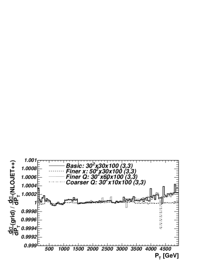
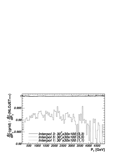
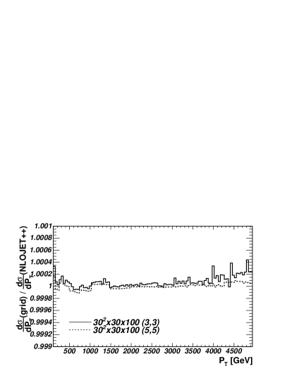
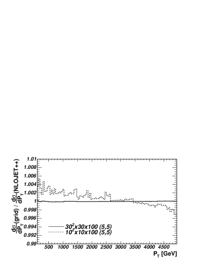
Figure 54: Ratio between the single inclusive jet cross-section with $100$ $P_{T}$ bins calculated with the grid technique and the reference cross-section calculated in the standard way. Shown are the standard grid, grids with finer $x$ and $Q^{2}$ sampling (a) with interpolation of order $1$, $3$ and $5$ (b) (and on a finer scale in c)) and a small grid (d).

We have developed a technique to store the perturbative coefficients calculated by an NLO Monte Carlo program on a grid allowing for a-posteriori inclusion of an arbitrary parton density function (PDF) set. We extended a technique that was already successfully used to analyse HERA data to the more demanding case of proton-proton collisions at LHC energies.

The technique can be used to constrain PDF uncertainties, e.g. at high momentum transfers, from data that will be measured at LHC and allows the consistent inclusion of final state observables in global QCD analyses. This will help increase the sensitivity of LHC to find new physics as deviations from the Standard Model predictions.

Even for the large kinematic range for the parton momentum fractions $x_{1}$ and $x_{2}$ and of the squared momentum transfer $Q^{2}$ accessible at LHC, grids of moderate size seem to be sufficient. The single inclusive jet cross-section in the central region $|y|<0.5$ can be calculated with a precision of $0.01\%$ in a realistic example with $100$ bins in the transverse jet energy range $100\,\leq P_{T}\leq 5000\,\mathrm{GeV}$. In this example, the grid occupies about $300$ Mbyte computer memory. With smaller grids of order $10$ Mbyte the reachable accuracy is still $0.5\%$. This is probably sufficient for all practical applications.

4 GLAP evolution and parton fits

4.1 Introduction

The high-precision data from HERA and the anticipated data from LHC open the possibility for a precise determination of parton distributions. This, however, requires an improvement in the theoretical description of DIS and hard hadronic scattering processes, as well as an improvement of the techniques used to extract parton distributions from the data.

The determination of perturbative QCD corrections has undergone substantial progress recently. The key ingredient of a complete next-to-next-to-leading order (NNLO) prediction in perturbative QCD are the recently calculated three-loop splitting functions which govern the scale dependence of PDFs. Extensions in the accuracy of the perturbative predictions yet beyond NNLO are given by the three-loop coefficient functions for $F_{2}$, while the coefficient functions for $F_{L}$ at this order are actually required to complete the NNLO predictions. Section 4.2 briefly discusses the recent results and their phenomenological implications. Certain mathematical aspects, which are important in the calculation of higher order corrections in massless QCD are presented in section 4.3. In particular, algebraic relations in Mellin-$N$ space are pointed out, which are of importance for harmonic sums, harmonic polylogarithms and multiple $\zeta$-values.

These calculation of the PDF evolution to NNLO in perturbative QCD are used in section 4.4 to provide an update and extension of a set of benchmark tables for the evolution of parton distributions of hadrons. These benchmark tables were first presented in the report of the QCD/SM working group at the 2001 Les Houches workshop, but based on approximate NNLO splitting functions, which are superseded by the exact results which are now available. In addition, section 4.4 now includes also reference tables for the case of polarized PDF evolution.

Whereas in principle the $x$-shapes of PDFs at low scales can be determined from first principles using non-perturbative methods, in practice at present this is only possible using models (briefly touched in in section 4.5). Therefore, an accurate determination of PDFs requires a global QCD fit to the data, which is the subject of sections 4.6–59.

Section 4.6 discusses in particular the impact on parton fits of NNLO corrections on the one hand, and of the inclusion of Drell-Yan data and future LHC data on the other hand. It then presents values for a benchmark fit together with a table of correlation coefficients for the parameter obtained in the fit. This benchmark fit is then re-examined in sec. 4.7, along with a comparison between PDFs and the associated uncertainty obtained using the approaches of Alekhin and the MRST group. The differences between these benchmark partons and the actual global fit partons are also discussed, and used to explore complications inherent in extracting PDFs with uncertainties. Finally, in section 59 the stability of PDF determinations in NLO global analyses is re-investigated and the results of the CTEQ PDF group on this issue are summarized.

An alternative approach to a completely bias-free parameterization of PDFs is presented in section 4.9. There, a neural network approach to global fits of parton distribution functions is introduced and work on unbiased parameterizations of deep-inelastic structure functions with faithful estimation of their uncertainties is reviewed together with a summary of the current status of neural network parton distribution fits.

4.2 Precision Predictions for Deep-Inelastic Scattering

With high-precision data from HERA and in view of the outstanding importance of hard scattering processes at the LHC, a quantitative understanding of deep-inelastic processes is indispensable, necessitating calculations beyond the standard next-to-leading order of perturbative QCD.

In this contribution we review recent results for the complete next-to-next-to-leading order (NNLO, N²LO) approximation of massless perturbative QCD for the structure functions $F_{\,1}$, $F_{\,2}$, $F_{\,3}$ and $F_{L}$ in DIS. These are based on the second-order coefficient functions [103, 104, 105, 106, 107], the three-loop splitting functions which govern the evolution of unpolarized parton distributions of hadrons [108, 109] and the three-loop coefficient functions for $F_{L}=F_{\,2}-2xF_{1}$ in electromagnetic (photon-exchange) DIS [63, 110]. Moreover we discuss partial N³LO results for $F_{2}$, based on the corresponding three-loop coefficient functions also presented in Ref. [110]. For the splitting functions $P$ and coefficient functions $C$ we employ the convention

$$P(\alpha_{\rm s})\,=\,\sum_{n=0}\,\left(\frac{\alpha_{\rm s}}{4\pi}\right)^{n+1}P^{(n)}\,,\quad\quad\quad C(\alpha_{\rm s})\,=\,\sum_{n=0}\,\left(\frac{\alpha_{\rm s}}{4\pi}\right)^{n}C^{(n)}$$ (38)

for the expansion in the running coupling constant $\alpha_{\rm s}$. For the longitudinal structure function $F_{L}$ the third-order corrections are required to complete the NNLO predictions, since the leading contribution to the coefficient function $C_{L}$ is of first order in the strong coupling constant $\alpha_{\rm s}$.

In the following we briefly display selected results to demonstrate the quality of precision predictions for DIS and their effect on the evolution. The exact (analytical) results to third order for the quantities in Eq. (38) are too lengthy, about ${\cal O}(100)$ pages in normalsize fonts and will not be reproduced here. Also the method of calculation is well documented in the literature [107, 111, 108, 109, 110, 112]. In particular, it proceeds via the Mellin transforms of the functions of the Bjorken variable $x$,

$$A(N) = \int\limits_{0}^{1}\!dx\>x^{N-1}A(x)\,.$$ (39)

Selected mathematical aspects of Mellin transforms are discussed in section 4.3.

4.2.1 Parton evolution

The well-known $2n_{f}-1$ scalar non-singlet and $2\times 2$ singlet evolution equations for $n_{f}$ flavors read

$$\frac{d}{d\ln\mu_{f}^{\,2}}\>q_{\rm ns}^{\>i}\>=\>P_{\rm ns}^{\,i}\,\otimes\,q_{\rm ns}^{\,i}\,,\,\,\,\,\,\,\,\,\,\,\,\,\,\,\,\,\,i=\pm,\mbox{v}\>,$$ (40)

for the quark flavor asymmetries $q_{\rm ns}^{\pm}$ and the valence distribution $q_{\rm ns}^{\rm v}$, and

$$\frac{d}{d\ln\mu_{f}^{\,2}}\left(\begin{array}[]{c}\!q_{\rm s}\!\\ g\end{array}\right)\>=\>\left(\begin{array}[]{cc}P_{\rm qq}&P_{\rm qg}\\ P_{\rm gq}&P_{\rm gg}\end{array}\right)\otimes\left(\begin{array}[]{c}\!q_{\rm s}\!\\ g\end{array}\right)$$ (41)

for the singlet quark distribution $q_{\rm s}$ and the gluon distribution $g$, respectively. Eqs. (40) and (41) are governed by three independent types of non-singlet splitting functions, and by the $2\times 2$ matrix of singlet splitting functions. Here $\otimes$ stands for the Mellin convolution. We note that benchmark numerical solutions to NNLO accuracy of Eqs. (40) and (41) for a specific set of input distributions are given in section 4.4. Phenomenological QCD fits of parton distributions in data analyses are extensively discussed in sections 4.6–59. An approach based on neural networks is described in section 4.9.

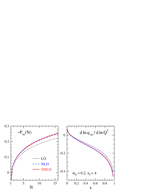
Figure 55: On the left we show the perturbative expansion of $P_{\,\rm ns}^{\,\rm v}(N)$, and on the right the resulting perturbative expansion of the logarithmic scale derivative $\,d\ln q_{\,\rm ns}/d\ln\mu_{f}^{\,2}\,$ is displayed for a model input. See the text for details.

Let us start the illustration of the precision predictions by looking at the parton evolution and at large Mellin-$N$ (large Bjorken-$x$) behavior. Fig. 55 shows the stability of the perturbative expansion which is very benign and indicates, for $\alpha_{\rm s}\raisebox{-1.9919pt}{$\>\>\stackrel{{\scriptstyle<}}{{{\scriptstyle\sim}}}\>\>$}0.2$, corrections of less than 1% beyond NNLO. On the left we show the results for the perturbative expansion of $P_{\rm ns}$ in Mellin space, cf. Eqs. (38), (39). We employ four active flavors, $n_{f}=4$, and an order-independent value for the strong coupling constant,

$$\alpha_{\rm s}(\mu_{0}^{\,2})\>=\>0.2\>\>,$$ (42)

which corresponds to $\mu_{0}^{\,2}\,\simeq\,25\ldots 50$ GeV² for $\alpha_{\rm s}(M_{Z}^{\,2})=0.114\ldots 0.120$ beyond the leading order. On the right of Fig. 55 the perturbative expansion of the logarithmic derivative, cf. Eqs. (38), (40), is illustrated at the standard choice $\mu_{r}=\mu_{f}$ of the renormalization scale. We use the schematic, but characteristic model distribution,

$$xq_{\,\rm ns}(x,\mu_{0}^{\,2}) = x^{\,0.5}(1-x)^{3}\,.$$ (43)

The normalization of $q_{\,\rm ns}$ is irrelevant at this point, as we consider the logarithmic scale derivative only.

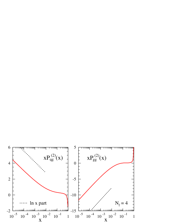
Figure 56: The three-loop gluon-quark (left) and gluon-gluon (right) splitting functions together with the leading small-$x$ contribution (dotted line).

Next, let us focus on the three-loop splitting functions at small momentum fractions $x$, where the splitting functions $P_{\,\rm ig}$ in the lower row of the $2\times 2$ matrix in Eq. (41), representing $\rm g\!\rightarrow\!i$ splittings, are most important. In Fig. 56 we show, again for $n_{f}=4$, the three-loop splitting functions $P^{(2)}_{\,\rm qg}$ and $P^{(2)}_{\,\rm gg}$ together with the leading small-$x$ term indicated separately for $x<0.01$. In the present singlet case the leading logarithmic small-$x$ limits $\sim x^{\,-1}\ln x$ of Refs. [113, 114] are confirmed together with the general structure of the BFKL limit [29, 30, 115]. The same holds for the leading small-$x$ terms $\ln^{4}x$ in the non-singlet sector [116, 117], with the qualification that a new, unpredicted leading logarithmic contribution is found for the color factor $d^{abc}d_{abc}$ entering at three loops for the first time.

It is obvious from Fig. 56 (see also Refs. [107, 108, 109, 112]) that the leading $\>x\!\rightarrow 0$-terms alone are insufficient for collider phenomenology at HERA or the LHC as they do not provide good approximations of the full results at experimentally relevant small values of $x$. Resummation of the small-$x$ terms and various phenomenological improvements are discussed in detail in section 5.

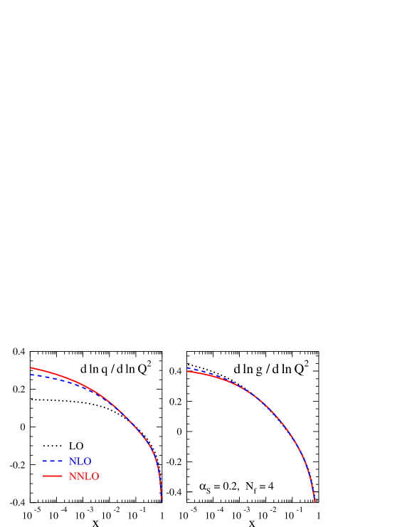
Figure 57: The perturbative expansion of the scale derivatives (41) of the singlet distributions (4.2.1).

In the same limit of small $x$, it is instructive to look at the evolution of parton distributions. Again, we choose the reference scale of Eq. (42), $n_{f}=4$ and the sufficiently realistic model distributions

$$xq_{\rm s}(x,\mu_{0}^{\,2}) \!=\! 0.6\>x^{\,-0.3}(1-x)^{3.5}\,(1+5.0\>x^{\,0.8\,})$$

$$xg(x,\mu_{0}^{\,2})\>\> \!=\! 1.6\>x^{\,-0.3}(1-x)^{4.5}\,(1-0.6\>x^{\,0.3\,})$$ (44)

irrespective of the order of the expansion to facilitate direct comparisons of the various contributions. Of course, this order-independence does not hold for actual data-fitted parton distributions like those in sections 4.6–59. In Fig. 57 we display the perturbative expansion of the scale derivative for the singlet quark and gluon densities at $\,\mu_{f}^{\,2}\>=\>\mu_{0}^{\,2\,}$ for the initial conditions specified in Eqs. (42) and (4.2.1). For the singlet quark distribution the total NNLO corrections, while reaching 10% at $x=10^{\,-4}$, remain smaller than the NLO results by a factor of eight or more over the full $x$-range. For the gluon distribution already the NLO corrections are small and the NNLO contribution amounts to only 3% for $x$ as low as $10^{\,-4}$. Thus, we see in Fig. 57 that the perturbative expansion is very stable. It appears to converge rapidly at $x>~{}10^{-3}$, while relatively large third-order corrections are found for very small momenta $\>x\raisebox{-1.9919pt}{$\>\>\stackrel{{\scriptstyle<}}{{{\scriptstyle\sim}}}\>\>$}10^{-4}$.

4.2.2 Coefficient functions

While the previous considerations were addressing the evolution of parton distributions, we now turn to the further improvements of precision predictions due to the full third-order coefficient functions for the structure functions $F_{2}$ and $F_{L}$ in electromagnetic DIS [63, 110]. The results for $F_{L}$ complete the NNLO description of unpolarized electromagnetic DIS, and the third-order coefficient functions for $F_{\,2}$ form, at not too small values of the Bjorken variable $x$, the dominant part of the next-to-next-to-next-to-leading order (N³LO) corrections. Thus, they facilitate improved determinations of the strong coupling $\alpha_{\rm s}$ from scaling violations.

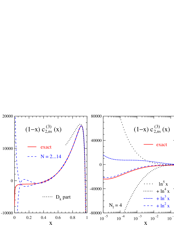
Figure 58: The three-loop non-singlet coefficient function $c_{\,2,\rm ns}^{\,(3)}(x)$ in the large-$x$ (left) and the small-$x$ (right) region, multiplied by $(1\!-\!x)$ for display purposes.

Let us start with the three-loop coefficient functions for $F_{2}$ in the non-singlet case. In Fig. 58 we display the three-loop non-singlet coefficient function $c_{\,2,\rm ns}^{\,(3)}(x)$ for $n_{f}=4$ flavors. We also show the soft-gluon enhanced terms ${\cal D}_{k}$ dominating the large-$x$ limit,

$${\cal D}_{k} = {\ln^{\,2k-1}(1-x)\over(1-x)_{+}}\,,$$ (45)

and the small-$x$ approximations obtained by successively including enhanced logarithms $\ln^{k}x$. However the latter are insufficient for an accurate description of the exact result. The dashed band in Fig. 58 shows the uncertainty of previous estimates [118] mainly based on the calculation of fixed Mellin moments [119, 120, 121]. For a detailed discussion of the soft-gluon resummation of the the ${\cal D}_{k}$ terms, we refer to section 5.

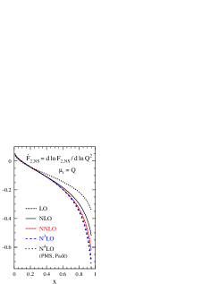
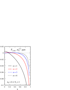
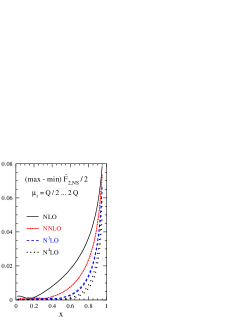
Figure 59: The perturbative expansion of the logarithmic scale derivative of the non-singlet structure function $F_{2,\rm ns}$. The results up to NNLO are exact, while those at N³LO are very good approximations. The N⁴LO corrections have been estimated by various methods.

Building on the coefficient functions, it is interesting to study the perturbative expansion of the logarithmic scale derivative for the non-singlet structure function $F_{2,\rm ns}$. To that end we use in Fig. 59 again the input shape Eq. (43) (this time for $F_{2,\rm ns}$ itself) irrespective of the order of the expansion, $n_{f}=4$ flavors and the reference scale of Eq. (42). The N⁴LO approximation based on Padé summations of the perturbation series can be expected to correctly indicate at least the rough size of the four-loop corrections, see Ref. [110] for details. From Fig. 59 we see that the three-loop results for $F_{\,2}$ can be employed to effectively extend the main part of DIS analyses to the N³LO at $x>10^{-2}$ where the effect of the unknown fourth-order splitting functions is expected to be very small. This has, for example, the potential for a ‘gold-plated’ determination of $\alpha_{\rm s}(M_{Z})$ with an error of less than 1% from the truncation of the perturbation series. On the right hand side of Fig. 59 the scale uncertainty which is conventionally estimated by

$$\Delta\dot{f} \equiv {1\over 2}\,\left(\max\,[\dot{f}(x,\mu_{r}^{2})]-\min\,[\dot{f}(x,\mu_{r}^{2})]\right)\,,$$ (46)

is plotted, where the scale varies $\mu_{r}\in[Q/2,2Q]$.

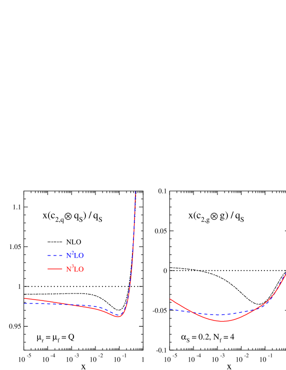
Figure 60: The perturbative expansion up to three loops (N³LO) of the quark (left) and gluon (right) contributions to singlet structure function $F_{2}$.

In the singlet case, we can study the quark and gluon contributions to the structure function $F_{2}$. In Fig. 60 we plot the perturbative expansion up to N³LO of the quark and gluon contributions to structure function $F_{2,\rm s}$ at the scale (42) using the distributions (4.2.1). All curves have been normalized to the leading-order result $\,F_{2,\rm s}^{\,\rm LO}=\langle e^{2}\rangle\>q_{\rm s}\,$. Fig. 60 nicely illustrates the perturbative stability of the structure function $F_{2}$.

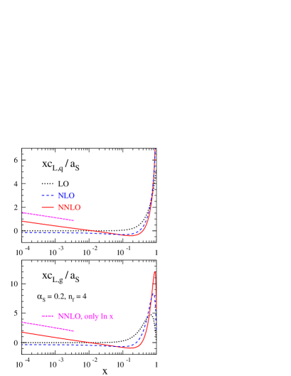
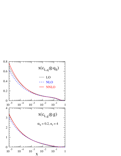
Figure 61: The perturbative expansion to N²LO of the longitudinal singlet-quark and gluon coefficient functions to third order multiplied by $x$ for display purposes (left) and of the quark and gluon contributions to singlet structure function $F_{L}$ (right).

Finally, we address the longitudinal structure function $F_{L}$ at three loops. In the left part of Fig. 61 we plot the singlet-quark and gluon coefficient functions $c_{L,\rm q}$ and $c_{L,\rm g}$ for $F_{L}$ up to the third order for four flavors and the $\alpha_{\rm s}$-value of Eq. (42). The curves have been divided by $a_{\rm s}=\alpha_{s}/(4\pi)$ to account for the leading contribution being actually of first order in the strong coupling constant $\alpha_{\rm s}$. Both the second-order and the third-order contributions are rather large over almost the whole $x$-range. Most striking, however, is the behavior at very small values of $x$, where the anomalously small one-loop parts are negligible against the (negative) constant two-loop terms, which in turn are completely overwhelmed by the (positive) new three-loop corrections $xc_{L,a}^{(3)}\sim\ln x\,+\,$const , which we have indicated in Fig. 61.

To assess the effect for longitudinal structure function $F_{L}$, we convolute in Fig. 61 on the right the coefficient functions with the input shapes Eq. (4.2.1) for $n_{f}=4$ flavors and the reference scale of Eq. (42). A comparison of the left and right plots in Fig. 61 clearly reveals the smoothening effect of the Mellin convolutions. For the chosen input conditions, the (mostly positive) NNLO corrections to the flavor-singlet $F_{L}$ amount to less than 20% for $5\cdot 10^{-5}<x<0.3$. In data fits we expect that the parton distributions, in particular the gluon distribution, will further stabilize the overall NNLO/NLO ratio. Thus, at not too small scales, $F_{L}$ is a quantity of good perturbative stability, for the $x$-values accessible at HERA, see Ref. [63] for more details.

4.3 Mathematical Structure of Higher Order Corrections

The QCD anomalous dimensions and Wilson coefficients for structure functions are single scale quantities and may be expressed in simple form in Mellin space in terms of polynomials of harmonic sums and ration functions of the Mellin variable. Unlike the case in various calculations using representations in momentum-fraction ($z$-) space the use of multiple nested harmonic sums leads to a synchronization in language. Furthermore, significant simplifications w.r.t. the number of functions needed can be achieved. This is due to algebraic [122, 123] relations between these quantities, which in a similar way are also present between harmonic polylogarithms [124] and multiple $\zeta$-values [125]. These relations result from the the specific index pattern of the objects considered and their multiplication relation and do not refer to further more specific properties. In Table 13 we illustrate the level of complexity which one meets in case of harmonic sums. To three–loop order weight w=6 harmonic sums occur. The algebraic relations for the whole class of harmonic sums lead to a reduction by a factor of $\sim 4$ (column 3). As it turns out, physical pseudo-observables, as anomalous dimensions and Wilson-coefficients in the $\overline{\rm MS}$ scheme, to 2– resp. 3–loop order depend on harmonic sums only, in which the index $\{-1\}$ never occurs. The algebraic reduction for this class is illustrated in column 5. We also compare the complexity of only non-alternating harmonic sums and their algebraic reduction, which is much lower. This class of sums is, however, not wide enough to describe the above physical quantities. In addition to the algebraic relations of harmonic sums structural relations exist, which reduces the basis further [126].

Table 13: Number of alternating and non-alternating harmonic sums in dependence of their weight, [126].

Using all these relations one finds that 5 basic functions are sufficient to describe all 2–loop Wilson coefficients for deep–inelastic scattering [127] and further 8 [128] for the 3–loop anomalous dimensions. Their analytic continuations to complex values of the Mellin variable are given in [129, 130]. These functions are the (regularized) Mellin transforms of :

$$\frac{\ln(1+x)}{1+x},\hskip 28.45274pt\frac{{\rm Li}_{2}(x)}{1\pm x},\hskip 28.45274pt\frac{S_{1,2}(x)}{1\pm x},\hskip 28.45274pt\frac{{\rm Li}_{4}(x)}{x\pm 1},$$

$$\frac{S_{1,3}(x)}{1+x},\hskip 28.45274pt\frac{S_{2,2}(x)}{x\pm 1},\hskip 39.83368pt\frac{{\rm Li}_{2}^{2}(x)}{1+x},\hskip 28.45274pt\frac{S_{2,2}(-x)-{\rm Li}_{2}^{2}(-x)/2}{x\pm 1}~{}.$$ (47)

It is remarkable, that the numerator–functions in (4.3) are Nielsen integrals [131] and polynomials thereof, although one might expect harmonic polylogarithms [124] outside this class in general. The representation of the Wilson coefficients and anomalous dimensions in the way described allows for compact expressions and very fast and precise numerical evaluation well suited for fitting procedures to experimental data.

4.3.1 Two–loop Processes at LHC in Mellin Space

Similar to the case of the Wilson coefficients in section 4.3 one may consider the Wilson coefficients for inclusive hard processes at hadron colliders, as the Drell–Yan process to $O(\alpha_{s}^{2})$ [132, 133, 134], scalar or pseudoscalar Higgs–boson production to $O(\alpha_{s}^{3})$ in the heavy–mass limit [135, 136, 137, 138, 139, 140], and the 2–loop time–like Wilson coefficients for fragmentation [141, 142, 143]. These quantities have been analyzed in [144, 145] w.r.t. their general structure in Mellin space. The cross section for the Drell–Yan process and Higgs production is given by

$$\sigma\left(\frac{\hat{s}}{s},Q^{2}\right)=\int_{x}^{1}\frac{dx_{1}}{x_{1}}\int_{x/x_{1}}^{1}\frac{dx_{2}}{x_{2}}f_{a}(x_{1},\mu^{2})f_{b}(x_{2},\mu^{2})\hat{\sigma}\left(\frac{x}{x_{1}x_{2}},\frac{Q^{2}}{\mu^{2}}\right)~{},$$ (4.48)

with $x=\hat{s}/s$. Here, $f_{c}(x,\mu^{2})$ are the initial state parton densities and $\mu^{2}$ denotes the factorization scale. The Wilson coefficient of the process is $\hat{\sigma}$ and $Q^{2}$ is the time–like virtuality of the $s$–channel boson. Likewise, for the fragmentation process of final state partons into hadrons in $pp$–scattering one considers the double differential final state distribution

$$\frac{d^{2}\sigma^{H}}{dxd\cos\theta}=\frac{3}{8}(1+\cos^{2}\theta)\frac{d\sigma_{T}^{H}}{dx}+\frac{3}{4}\sin^{2}\theta\frac{d\sigma_{L}^{H}}{dx}~{}.$$ (4.49)

Here,

$$\frac{d\sigma^{H}_{k}}{dx} = \int_{x}^{1}\frac{dz}{z}\Biggl{[}\sigma_{\rm tot}^{(0)}\left\{D_{S}^{H}\left(\frac{x}{z},M^{2}\right)C_{k,q}^{\rm S}(z,Q^{2}/M^{2})+D_{g}^{H}\left(\frac{x}{z},M^{2}\right)C_{k,q}^{\rm S}(z,Q^{2}/M^{2})\right\}$$ (4.50)

$$+\sum_{p=1}^{N_{f}}\sigma_{p}^{(0)}D_{{\rm NS},p}^{H}\left(\frac{x}{z},M^{2}\right)C_{k,q}^{\rm NS}(z,Q^{2}/M^{2})\Biggr{]}~{}.$$

In the subsystem cross-sections $\sigma$ the initial state parton distributions are included. $D_{k}^{H}$ denote the non–perturbative fragmentation functions and $C_{k,i}^{\rm S,NS}(z,Q^{2}/M^{2})$ the respective time–like Wilson coefficients describing the fragmentaion process for a parton $i$ into the hadron $H$.

Although these Wilson coefficients are not directly related to the 2–loop Wilson coefficients for deeply inelastic scattering, one finds for these functions at most the same set of basic functions as given above. Again one obtains very fast and concise numerical programs also for these processes working in Mellin space, which will be well suited for inclusive analyses of experimental collider data at LHC in the future.

4.3.2 Non–Singlet Parton Densities at $O(\alpha_{s}^{3})$

The precision determination of the QCD–scale $\Lambda_{\rm QCD}$ and of the idividual parton densities is an important issue for the whole physics programme at LHC since all measurements rely on the detailed knwoledge of this parameter and distribution functions. In Ref. [146] first results were reported of a world data analysis for charged lepton-$p(d)$ scattering w.r.t. the flavor non–singlet sector at $O(\alpha_{s}^{3})$ accuracy. The flavor non–singlet distributions $xu_{v}(x,Q^{2})$ and $xd_{v}(x,Q^{2})$ were determined along with fully correlated error bands giving parameterizations both for the values and errors of these distributions for a wide range in $x$ and $Q^{2}$. In Figure 62 these distributions including their error are shown. The value of the strong coupling constant $\alpha_{s}(M_{Z}^{2})$ was determined as $0.1135+0.0023-0.0026~{}(\rm exp.)$ The full analysis is given in [147], including the determination of higher twist contributions in the large $x$ region both for $F_{2}^{p}(x,Q^{2})$ and $F_{2}^{d}(x,Q^{2})$.

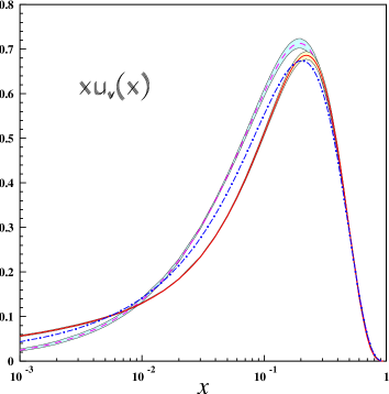
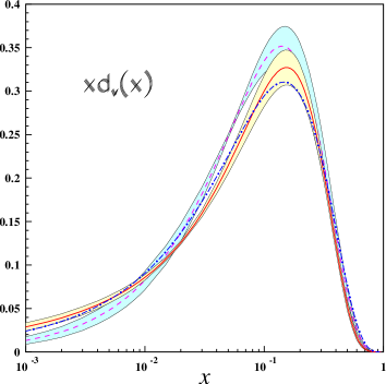
Figure 62: $xu_{v}$ and $xd_{v}$ at $Q_{0}^{2}=4{\rm GeV}^{2}$ (full lines) [146]; dashed lines [148]; dash-dotted lines [39].

4.3.3 Scheme-invariant evolution for unpolarzed DIS structure functions

The final HERA-II data on unpolarized DIS structure functions, combined with the present world data from other experiments, will allow to reduce the experimental error on the strong coupling constant, $\alpha_{s}(M_{Z}^{2})$, to the level of $1\%$ [149]. On the theoretical side the NLO analyzes have intrinsic limitations which allow no better than $5$% accuracy in the determination of $\alpha_{s}$ [150]. In order to match the expected experimental accuracy, analyzes of DIS structure functions need then to be carried out at the NNLO–level. To perform a full NNLO analysis the knowledge of the 3-loop $\beta$-function coefficient, $\beta_{2}$, the 2– resp. 3–loop Wilson coefficients and the 3-loop anomalous dimensions is required. With the calculation of the latter [108, 109], the whole scheme–independent set of quantities is known, thus allowing a complete NNLO study of DIS structure functions.

Besides the standard approach solving the QCD evolution equations for parton densities in the $\overline{\rm MS}$ scheme it appears appealing to study scheme–invariant evolution equations [151]. Within this approach the input distributions at a scale $Q^{2}_{0}$ are measured experimentally. The only parameter to be determined by a fit to data is the QCD–scale $\Lambda_{\rm QCD}$. To perform an analysis in the whole kinematic region the non–singlet [146] contribution has to be separated from the singlet terms of two measured observables. In practice these can be chosen to be $F_{2}(x,Q^{2})$ and $\partial F_{2}(x,Q^{2})/\partial\ln(Q^{2})$ or $F_{2}(x,Q^{2})$ and $F_{L}(x,Q^{2})$ if the latter structure function is measured well enough. Either $\partial F_{2}(x,Q^{2})/\partial\ln(Q^{2})$ or $F_{L}(x,Q^{2})$ play a role synonymous to the gluon distribution while $F_{2}(x,Q^{2})$ takes the role of the singlet–quark distribution compared to the standard analysis. These equations do no longer describe the evolution of universal quantities depending on the choice of a scheme but of process–dependent quantities which are observables and thus factorization scheme–indedependent. Since the respective evolution kernels are calculated in perturbation theory the dependence on the renormalization scale remains and becomes smaller with the order in the coupling constant included.

Physical evolution kernels have been studied before in [152, 153, 154]. The 3–loop scheme–invariant evolution equations were solved in the massless case in [151]. This analysis is extended including the heavy flavor contributions at present [147]. The large complexity of the evolution kernels can only be handeled in Mellin space since in $z$–space various inverse and direct Mellin convolutions would be required numerically, causing significant accuracy and run–time problems. The inclusion of the heavy flavor contributions is possible using the parameterizations [155].

In Fig. 62 we present the scheme invariant evolution for the structure functions $F_{2}$ and $\partial F_{2}/\partial t$ to NNLO with $t=-2/\beta_{0}\ln(\alpha_{s}(Q^{2})/\alpha_{s}(Q_{0}^{2}))$. The input distribution at the reference scale are not extracted from data, but rather built up as a convolution of Wilson coefficients and PDFs, the latter being parametrised according to [156].

Figure 63: NNLO scheme invariant evolution for the singlet part of the structure function $F_{2}$ and its slope $\partial F_{2}/\partial t$ for four massless flavours, [151].

Scheme–invariant evolution equations allow a widely un–biased approach to determine the initial conditions for QCD evolution, which in general is a source of systematic effects which are difficult to control. On the other hand, their use requires to consider all correlations of the input measurements in a detailed manner experimentally. At any scale $Q^{2}$ mappings are available to project the observables evolved onto the quark–singlet and the gluon density in whatever scheme. In this way the question whether sign changes in the unpolarized gluon distribution in the $\overline{\rm MS}$ scheme do occur or do not occur in the small $x$ region can be answered uniquely. As in foregoing analyses [157, 146] correlated error propagation throughout the evolution is being performed.

4.4 Updated reference results for the evolution of parton distributions 

In this contribution we update and extend our benchmark tables, first presented in the report of the QCD/SM working group at the 2001 Les Houches workshop [156], for the evolution of parton distributions of hadrons in perturbative QCD. Since then the complete next-to-next-to-leading order (NNLO) splitting functions have been computed [108, 109], see also section 4.2. Thus we can now replace the NNLO results of 2001 which were based on the approximate splitting functions of Ref. [158]. Furthermore we now include reference tables for the polarized case treated in neither Ref. [156] nor the earlier study during the 1995/6 HERA workshop [159]. Since the spin-dependent NNLO splitting functions are still unknown, we have to restrict ourselves to the polarized leading-order (LO) and next-to-leading-order (NLO) evolution.

As in Ref. [156], we employ two entirely independent and conceptually different Fortran programs. At this point, the $x$-space code of G.S. is available from the author upon request, while the Mellin-space program of A.V. has been published in Ref. [160]. The results presented below correspond to a direct iterative solution of the N^mLO evolution equations for the parton distributions $f_{p}(x,\mu_{\rm f}^{2})\equiv p(x,\mu_{\rm f}^{2})$, where $p=q_{i},\,\bar{q}_{i}\,,g$ with $i=1,\,\ldots,N_{\rm f}$,

$$\frac{d\>\!f_{p}(x,\mu_{\rm f}^{2})}{d\ln\mu_{\rm f}^{2}}\>=\>\sum_{l=0}^{m}\,a_{\rm s}^{\,l+1}(\mu_{\rm r}^{2})\int_{x}^{1}\!\frac{dy}{y}\,\sum_{p^{\prime}}\>\!P_{pp^{\prime}}^{(l)}\bigg{(}\frac{x}{y},\frac{\mu_{\rm f}^{2}}{\mu_{\rm r}^{2}}\bigg{)}\,f_{p^{\prime}}(y,\mu_{\rm f}^{2})$$ (4.51)

with the strong coupling, normalized as $a_{\rm s}\equiv\alpha_{\rm s}/(4\pi)$, given in terms of

$$\frac{d\,a_{\rm s}}{d\ln\mu_{r}^{2}}\>=\>\beta_{\rm N^{m}LO}(a_{\rm s})\>=\>-\sum_{l=0}^{m}\,a_{\rm s}^{\,l+2}\,\beta_{\>\!l}$$ (4.52)

with $\,\beta_{0}=11-2/3\,N_{\rm f}\,$ etc. $\mu_{\rm r}$ and $\mu_{\rm f}$ represent the renormalization and mass-factorization scales in the $\overline{\mbox{MS}}$ scheme. The reader is referred to Refs. [156, 160] for the scale dependence of the splitting functions $P^{(l)}$ and a further discussion of our solutions of Eqs. (4.51) and (4.52).

For the unpolarized case we retain the initial conditions as set up at the Les Houches meeting: The evolution is started at

$$\mu_{\rm f,0}^{2}\>=\>2\mbox{ GeV}^{2}\>\>.$$ (4.53)

Roughly along the lines of the CTEQ5M parametrization [161], the input distributions are chosen as

$$xu_{\rm v}(x,\mu_{\rm f,0}^{2}) \!=\! 5.107200\>x^{0.8}\>(1-x)^{3}$$

$$xd_{\rm v}(x,\mu_{\rm f,0}^{2}) \!=\! 3.064320\>x^{0.8}\>(1-x)^{4}$$

$$xg\,(x,\mu_{\rm f,0}^{2}) \!=\! 1.700000\,x^{-0.1}(1-x)^{5}$$ (4.54)

$$x\bar{d}\,(x,\mu_{\rm f,0}^{2}) \!=\! .1939875\,x^{-0.1}(1-x)^{6}$$

$$x\bar{u}\,(x,\mu_{\rm f,0}^{2}) \!=\! (1-x)\>x\bar{d}\,(x,\mu_{\rm f,0}^{2})$$

$$xs\,(x,\mu_{\rm f,0}^{2}) \!=\! x\bar{s}\,(x,\mu_{\rm f,0}^{2})\>=\>0.2\,x(\bar{u}+\bar{d}\,)(x,\mu_{\rm f,0}^{2})$$

where, as usual, $q_{i,\rm v}\equiv q_{i}-\bar{q}_{i}$. The running couplings are specified by Eq. (4.52) and

$$\alpha_{\rm s}(\mu_{\rm r}^{2}\!=\!2\mbox{ GeV}^{2})\>=\>0.35\>\>.$$ (4.55)

For simplicity initial conditions (4.4) and (4.55) are employed regardless of the order of the evolution and the (fixed) ratio of the renormalization and factorization scales.

For the evolution with a fixed number $N_{\rm f}>3$ of quark flavours the quark distributions not specified in Eq. (4.4) are assumed to vanish at $\mu_{\rm f,0}^{2}$, and Eq. (4.55) is understood to refer to the chosen value of $N_{\rm f}$. For the evolution with a variable $N_{\rm f}=3\ldots 6$, Eqs. (4.53) and (4.4) always refer to three flavours. $N_{\rm f}$ is then increased by one unit at the heavy-quark pole masses taken as

$$m_{\rm c}\>=\>\mu_{\rm f,0}\>,\quad m_{\rm b}\>=\>4.5\mbox{ GeV}^{2}\>,\quad m_{\rm t}\>=\>175\mbox{ GeV}^{2}\>\>,$$ (4.56)

i.e., Eqs. (4.51) and (4.52) are solved for a fixed number of flavours between these thresholds, and the respective matching conditions are invoked at $\mu_{\rm f}^{2}=m_{\rm h\,}^{2}$, $\,h=c,\,b,\,t$. The matching conditions for the unpolarized parton distributions have been derived at NNLO in Ref. [162], and were first implemented in an evolution program in Ref. [163]. Note that, while the parton distributions are continuous up to NLO due to our choice of the matching scales, $\alpha_{\rm s}$ is discontinuous at these flavour thresholds already at this order for $\mu_{\rm r}\neq\mu_{\rm f}$, see Refs. [164, 165]. Again the reader is referred to Refs. [156, 160] for more details.

Since the exact NNLO splitting functions $P^{(2)}$ are rather lengthy and not directly suitable for use in a Mellin-space program (see, however, Ref. [130]), the reference tables shown below have been computed using the parametrizations (4.22) – (4.24) of Ref. [108] and (4.32) – (4.35) of Ref. [109]. Likewise, the operator matrix element $\widetilde{A}_{\rm hg}^{\rm S,2}$ entering the NNLO flavour matching is taken from Eq. (3.5) of Ref. [160]. The relative error made by using the parametrized splitting functions is illustrated in Fig. 64. It is generally well below $10^{-4}$, except for the very small sea quark distributions at very large $x$.

Figure 64: Relative effects of using the parametrized three-loop splitting functions of Refs. [108, 109], instead of the exact expressions from the same source, on the NNLO evolution for the input (4.53) – (4.55) at two representative values of $\mu=\mu_{\rm r}=\mu_{\rm f}$.

Figure 65: Relative errors made by using the previous average approximations [158] for the three-loop splitting functions (used, e.g., in Refs. [39, 40]) instead of the full results [108, 109], on the NNLO evolution of the input (4.53) – (4.55) at $\,\mu_{\rm r}=\mu_{\rm f}$.

Eqs. (4.53), (4.55) and (4.56) are used for the (longitudinally) polarized case as well, where Eq. (4.4) replaced by the sufficiently realistic toy input [160]

$$xu_{\rm v} \!=\! +1.3\>x^{0.7}\>(1-x)^{3}\>(1+3x)$$

$$xd_{\rm v} \!=\! -0.5\>x^{0.7}\>(1-x)^{4}\>(1+4x)$$

$$xg\> \!=\! +1.5\>x^{0.5}\>(1-x)^{5}$$

$$x\bar{d}\> \!=\! x\bar{u}\>=\>-0.05\>x^{0.3}\>(1-x)^{7}$$

$$xs\> \!=\! x\bar{s}\>=\>+0.5\>x\bar{d}\>\>.$$ (4.57)

As Eq. (4.4) in the unpolarized case, this input is employed regardless of the order of the evolution.

As in Ref. [156], we have compared the results of our two evolution programs, under the conditions specified above, at 500 $x$-$\mu_{\rm f}^{2}$ points covering the range $10^{-8}\leq x\leq 0.9$ and $2\mbox{ GeV}^{2}\leq\mu_{\rm f}^{2}\leq 10^{6}\mbox{ GeV}^{2}$. A representative subset of our results at $\mu_{\rm f}^{2}=10^{4}\mbox{ GeV}^{4}$, a scale relevant to high-$E_{T}$ jets and close to $m_{\rm W}^{2}$, $m_{\rm Z}^{2}$ and, possibly, $m_{\rm Higgs}^{2}$, is presented in Tables 14 – 18. These results are given in terms of the valence distributions, defined below Eq. (4.4), $L_{\pm}\equiv\bar{d}\pm\bar{u}$, and the quark-antiquark sums $\,q_{+}\!\equiv q\!-\!\bar{q}\,$ for $\,q=s,\,c$ and, for the variable-$N_{\rm f}$ case, $b$.

For compactness an abbreviated notation is employed throughout the tables, i.e., all numbers $a\cdot 10^{b}$ are written as $a^{b}$. In the vast majority of the $x$-$\mu_{\rm f}^{2}$ points our results are found to agree to all five figures displayed, except for the tiny NLO and NNLO sea-quark distributions at $x=0.9$, in the tables. Entries where the residual offsets between our programs lead to a different fifth digit after rounding are indicated by the subscript ‘$*$’. In these cases the number with the smaller modulus is given in the tables.

The approximate splitting functions [158], as mentioned above employed in the previous version [156] of our reference tables, have been used in (global) NNLO fits of the unpolarized parton distributions [39, 40], which in turn have been widely employed for obtaining NNLO cross sections, in particular for $W$ and Higgs production. The effect of replacing the approximate results by the full splitting functions [108, 109] is illustrated in Figure 65. Especially at scales relevant to the above-mentioned processes, the previous approximations introduce an error of less than 0.2% for $x\!\raisebox{-1.9919pt}{$\>\>\stackrel{{\scriptstyle>}}{{{\scriptstyle\sim}}}\>\>$}\!10^{-3}$, and less than 1% even down to $\,x\simeq 10^{-5}$. Consequently the splitting-function approximations used for the evolution the parton distributions of Refs. [39, 40] are confirmed to a sufficient accuracy for high-scale processes at the LHC.

The unchanged unpolarized LO and NLO reference tables of Ref. [156] are not repeated here. Note that the one digit of the first (FFN) $\alpha_{\rm s}$ value was mistyped in the header of Table 1 in that report , the correct value can be found in Table 3 below.

Table 14: Reference results for the $N_{\rm f}\!=\!4$ next-next-to-leading-order evolution for the initial conditions (4.53) – (4.55). The corresponding value of the strong coupling is $\alpha_{\rm s}(\mu_{\rm r}^{2}\!=\!10^{4}\mbox{ GeV}^{2})=0.110141$. The valence distributions $s_{v}$ and $c_{v}$ are equal for the input (4.4). The notation is explained below Eq. (4.4) and in the paragraph below Eq. (4.4).

NNLO, $\,N_{\rm f}=4\,$, $\,\mu_{\rm f}^{2}=10^{4}\mbox{ GeV}^{2}$
$x$	$xu_{v}$	$xd_{v}$	$xL_{-}$	$2xL_{+}$	$xs_{v}$	$xs_{+}$	$xc_{+}$	$xg$
$\mu_{\rm r}^{2}=\mu_{\rm f}^{2}$
$\!10^{-7}\!$	$\!1.5287^{-4}\!$	$\!1.0244^{-4}\!$	$\!5.7018^{-6}\!$	$\!1.3190^{+2}\!$	$\!3.1437^{-5}\!$	$\!6.4877^{+1}\!$	$\!6.4161^{+1}\!$	$\!9.9763^{+2}\!$
$\!10^{-6}\!$	$\!6.9176^{-4}\!$	$\!4.4284^{-4}\!$	$\!2.5410^{-5}\!$	$\!6.8499^{+1}\!$	$\!9.4279^{-5}\!$	$\!3.3397^{+1}\!$	$\!3.2828^{+1}\!$	$\!4.9124^{+2}\!$
$\!10^{-5}\!$	$\!3.0981^{-3}\!$	$\!1.8974^{-3}\!$	$\!1.0719^{-4}\!$	$\!3.3471^{+1}\!$	$\!2.2790^{-4}\!$	$\!1.6059^{+1}\!$	$\!1.5607^{+1}\!$	$\!2.2297^{+2}\!$
$\!10^{-4}\!$	$\!1.3722^{-2}\!$	$\!8.1019^{-3}\!$	$\!4.2558^{-4}\!$	$\!1.5204^{+1}\!$	$\!3.6644^{-4}\!$	$\!7.0670^{+0}\!$	$\!6.7097^{+0}\!$	$\!9.0668^{+1}\!$
$\!10^{-3}\!$	$\!5.9160^{-2}\!$	$\!3.4050^{-2}\!$	$\!1.6008^{-3}\!$	$\!6.3230^{+0}\!$	$\!1.4479^{-4}\!$	$\!2.7474^{+0}\!$	$\!2.4704^{+0}\!$	$\!3.1349^{+1}\!$
$\!10^{-2}\!$	$\!2.3078^{-1}\!$	$\!1.2919^{-1}\!$	$\!5.5688^{-3}\!$	$\!2.2752^{+0}\!$	$\!-5.7311^{-4}\!$	$\!8.5502^{-1}\!$	$\!6.6623^{-1}\!$	$\!8.1381^{+0}\!$
$\!0.1\!$	$\!5.5177^{-1}\!$	$\!2.7165^{-1}\!$	$\!1.0023^{-2}\!$	$\!3.9019^{-1}\!$	$\!-3.0627^{-4}\!$	$\!1.1386^{-1}\!$	$\!5.9773^{-2}\!$	$\!9.0563^{-1}\!$
$\!0.3\!$	$\!3.5071^{-1}\!$	$\!1.3025^{-1}\!$	$\!3.0098^{-3}\!$	$\!3.5358^{-2}\!$	$\!-3.1891^{-5}\!$	$\!9.0480^{-3}\!$	$\!3.3061^{-3}\!$	$\!8.4186^{-2}\!$
$\!0.5\!$	$\!1.2117^{-1}\!$	$\!3.1528^{-2}\!$	$\!3.7742^{-4}\!$	$\!2.3867^{-3}\!$	$\!-2.7215^{-6}\!$	$\!5.7965^{-4}\!$	$\!1.7170^{-4}\!$	$\!8.1126^{-3}\!$
$\!0.7\!$	$\!2.0077^{-2}\!$	$\!3.0886^{-3}\!$	$\!1.3434^{-5}\!$	$\!5.4244^{-5}\!$	$\!-1.0106^{-7}\!$	$\!1.2936^{-5}\!$	$\!3.5304^{-6}\!$	$\!3.8948^{-4}\!$
$\!0.9\!$	$\!3.5111^{-4}\!$	$\!1.7783^{-5}\!$	$\!8.651^{-9}\!$	$\!2.695^{-8}\!$	$\!-1.476^{-10}\!$	$\!7.132^{-9}\!$	$\!2.990^{-9}\!$	$\!1.2136^{-6}\!$
$\mu_{\rm r}^{2}=2\,\mu_{\rm f}^{2}$
$\!10^{-7}\!$	$\!1.3416^{-4}\!$	$\!8.7497^{-5}\!$	$\!4.9751^{-6}\!$	$\!1.3020^{+2}\!$	$\!2.1524^{-5}\!$	$\!6.4025^{+1}\!$	$\!6.3308^{+1}\!$	$\!1.0210^{+3}\!$
$\!10^{-6}\!$	$\!6.2804^{-4}\!$	$\!3.9406^{-4}\!$	$\!2.2443^{-5}\!$	$\!6.6914^{+1}\!$	$\!6.5149^{-5}\!$	$\!3.2602^{+1}\!$	$\!3.2032^{+1}\!$	$\!4.9626^{+2}\!$
$\!10^{-5}\!$	$\!2.9032^{-3}\!$	$\!1.7575^{-3}\!$	$\!9.6205^{-5}\!$	$\!3.2497^{+1}\!$	$\!1.5858^{-4}\!$	$\!1.5570^{+1}\!$	$\!1.5118^{+1}\!$	$\!2.2307^{+2}\!$
$\!10^{-4}\!$	$\!1.3206^{-2}\!$	$\!7.7673^{-3}\!$	$\!3.9093^{-4}\!$	$\!1.4751^{+1}\!$	$\!2.5665^{-4}\!$	$\!6.8388^{+0}\!$	$\!6.4807^{+0}\!$	$\!9.0162^{+1}\!$
$\!10^{-3}\!$	$\!5.8047^{-2}\!$	$\!3.3434^{-2}\!$	$\!1.5180^{-3}\!$	$\!6.1703^{+0}\!$	$\!1.0388^{-4}\!$	$\!2.6695^{+0}\!$	$\!2.3917^{+0}\!$	$\!3.1114^{+1}\!$
$\!10^{-2}\!$	$\!2.2930^{-1}\!$	$\!1.2857^{-1}\!$	$\!5.4626^{-3}\!$	$\!2.2492^{+0}\!$	$\!-3.9979^{-4}\!$	$\!8.4058^{-1}\!$	$\!6.5087^{-1}\!$	$\!8.0993^{+0}\!$
$\!0.1\!$	$\!5.5428^{-1}\!$	$\!2.7326^{-1}\!$	$\!1.0072^{-2}\!$	$\!3.9297^{-1}\!$	$\!-2.1594^{-4}\!$	$\!1.1439^{-1}\!$	$\!5.9713^{-2}\!$	$\!9.0851^{-1}\!$
$\!0.3\!$	$\!3.5501^{-1}\!$	$\!1.3205^{-1}\!$	$\!3.0557^{-3}\!$	$\!3.6008^{-2}\!$	$\!-2.2632^{-5}\!$	$\!9.2227^{-3}\!$	$\!3.3771^{-3}\!$	$\!8.5022^{-2}\!$
$\!0.5\!$	$\!1.2340^{-1}\!$	$\!3.2166^{-2}\!$	$\!3.8590^{-4}\!$	$\!2.4459^{-3}\!$	$\!-1.9420^{-6}\!$	$\!5.9487^{-4}\!$	$\!1.7699^{-4}\!$	$\!8.2293^{-3}\!$
$\!0.7\!$	$\!2.0597^{-2}\!$	$\!3.1751^{-3}\!$	$\!1.3849^{-5}\!$	$\!5.5722^{-5}\!$	$\!-7.2616^{-8}\!$	$\!1.3244^{-5}\!$	$\!3.5361^{-6}\!$	$\!3.9687^{-4}\!$
$\!0.9\!$	$\!3.6527^{-4}\!$	$\!1.8544^{-5}\!$	$\!9.050^{-9}\!$	$\!2.663^{-8}\!$	$\!-1.075^{-10}\!$	$\!6.713^{-9}\!$	$\!2.377^{-9}\!$	$\!1.2489^{-6}\!$
$\mu_{\rm r}^{2}=1/2\,\mu_{\rm f}^{2}$
$\!10^{-7}\!$	$\!1.7912^{-4}\!$	$\!1.2521^{-4}\!$	$\!6.4933_{*}^{-6}\!$	$\!1.2714^{+2}\!$	$\!4.9649^{-5}\!$	$\!6.2498^{+1}\!$	$\!6.1784^{+1}\!$	$\!9.2473^{+2}\!$
$\!10^{-6}\!$	$\!7.7377^{-4}\!$	$\!5.1222^{-4}\!$	$\!2.8719^{-5}\!$	$\!6.7701^{+1}\!$	$\!1.4743^{-4}\!$	$\!3.2999^{+1}\!$	$\!3.2432^{+1}\!$	$\!4.6863^{+2}\!$
$\!10^{-5}\!$	$\!3.3184^{-3}\!$	$\!2.0760^{-3}\!$	$\!1.1977^{-4}\!$	$\!3.3644^{+1}\!$	$\!3.5445^{-4}\!$	$\!1.6147^{+1}\!$	$\!1.5696^{+1}\!$	$\!2.1747^{+2}\!$
$\!10^{-4}\!$	$\!1.4184^{-2}\!$	$\!8.4455^{-3}\!$	$\!4.6630^{-4}\!$	$\!1.5408^{+1}\!$	$\!5.6829^{-4}\!$	$\!7.1705^{+0}\!$	$\!6.8139^{+0}\!$	$\!8.9820_{*}^{+1}\!$
$\!10^{-3}\!$	$\!5.9793^{-2}\!$	$\!3.4418^{-2}\!$	$\!1.6996^{-3}\!$	$\!6.4042^{+0}\!$	$\!2.2278^{-4}\!$	$\!2.7892^{+0}\!$	$\!2.5128^{+0}\!$	$\!3.1336^{+1}\!$
$\!10^{-2}\!$	$\!2.3106^{-1}\!$	$\!1.2914^{-1}\!$	$\!5.7016^{-3}\!$	$\!2.2876^{+0}\!$	$\!-8.9125^{-4}\!$	$\!8.6205^{-1}\!$	$\!6.7377^{-1}\!$	$\!8.1589^{+0}\!$
$\!0.1\!$	$\!5.5039^{-1}\!$	$\!2.7075^{-1}\!$	$\!1.0031^{-2}\!$	$\!3.8850^{-1}\!$	$\!-4.7466^{-4}\!$	$\!1.1332^{-1}\!$	$\!5.9489^{-2}\!$	$\!9.0795^{-1}\!$
$\!0.3\!$	$\!3.4890^{-1}\!$	$\!1.2949^{-1}\!$	$\!2.9943^{-3}\!$	$\!3.5090^{-2}\!$	$\!-4.9304^{-5}\!$	$\!8.9667^{-3}\!$	$\!3.2670^{-3}\!$	$\!8.4309^{-2}\!$
$\!0.5\!$	$\!1.2026^{-1}\!$	$\!3.1269^{-2}\!$	$\!3.7428^{-4}\!$	$\!2.3729^{-3}\!$	$\!-4.1981^{-6}\!$	$\!5.7783^{-4}\!$	$\!1.7390^{-4}\!$	$\!8.1099_{*}^{-3}\!$
$\!0.7\!$	$\!1.9867^{-2}\!$	$\!3.0534^{-3}\!$	$\!1.3273^{-5}\!$	$\!5.4635^{-5}\!$	$\!-1.5541^{-7}\!$	$\!1.3275^{-5}\!$	$\!3.9930^{-6}\!$	$\!3.8824^{-4}\!$
$\!0.9\!$	$\!3.4524^{-4}\!$	$\!1.7466^{-5}\!$	$\!8.489^{-9}\!$	$\!3.030^{-8}\!$	$\!-2.255^{-10}\!$	$\!8.863^{-9}\!$	$\!4.803^{-9}\!$	$\!1.2026^{-6}\!$

Table 15: As Table 14, but for the variable-$N_{\rm f}$ evolution using the flavour matching conditions of Ref. [162, 164, 165]. The corresponding values for the strong coupling $\alpha_{\rm s}(\mu_{\rm r}^{2}\!=\!10^{4}\mbox{ GeV}^{2})$ are given by $0.115818$, $0.115605$ and $0.115410$ for $\mu_{\rm r}^{2}/\mu_{\rm f}^{2}=0.5$, $1$ and $2$, respectively. For brevity the small, but non-vanishing valence distributions $s_{v}$, $c_{v}$ and $b_{v}$ are not displayed.

NNLO, $\,N_{\rm f}=3\,\ldots 5\,$, $\,\mu_{\rm f}^{2}=10^{4}\mbox{ GeV}^{2}$
$x$	$xu_{v}$	$xd_{v}$	$xL_{-}$	$2xL_{+}$	$xs_{+}$	$xc_{+}$	$xb_{+}$	$xg$
$\mu_{\rm r}^{2}=\mu_{\rm f}^{2}$
$\!10^{-7}\!$	$\!1.5978^{-4}\!$	$\!1.0699^{-5}\!$	$\!6.0090^{-6}\!$	$\!1.3916^{+2}\!$	$\!6.8509^{+1}\!$	$\!6.6929^{+1}\!$	$\!5.7438^{+1}\!$	$\!9.9694^{+3}\!$
$\!10^{-6}\!$	$\!7.1787^{-4}\!$	$\!4.5929^{-4}\!$	$\!2.6569^{-5}\!$	$\!7.1710^{+1}\!$	$\!3.5003^{+1}\!$	$\!3.3849^{+1}\!$	$\!2.8332^{+1}\!$	$\!4.8817^{+2}\!$
$\!10^{-5}\!$	$\!3.1907^{-3}\!$	$\!1.9532^{-3}\!$	$\!1.1116^{-4}\!$	$\!3.4732^{+1}\!$	$\!1.6690^{+1}\!$	$\!1.5875^{+1}\!$	$\!1.2896^{+1}\!$	$\!2.2012^{+2}\!$
$\!10^{-4}\!$	$\!1.4023^{-2}\!$	$\!8.2749^{-3}\!$	$\!4.3744^{-4}\!$	$\!1.5617^{+1}\!$	$\!7.2747^{+0}\!$	$\!6.7244^{+0}\!$	$\!5.2597^{+0}\!$	$\!8.8804^{+1}\!$
$\!10^{-3}\!$	$\!6.0019^{-2}\!$	$\!3.4519^{-2}\!$	$\!1.6296^{-3}\!$	$\!6.4173^{+0}\!$	$\!2.7954^{+0}\!$	$\!2.4494^{+0}\!$	$\!1.8139^{+0}\!$	$\!3.0404^{+1}\!$
$\!10^{-2}\!$	$\!2.3244^{-1}\!$	$\!1.3000^{-1}\!$	$\!5.6100^{-3}\!$	$\!2.2778^{+0}\!$	$\!8.5749^{-1}\!$	$\!6.6746^{-1}\!$	$\!4.5073^{-1}\!$	$\!7.7912^{+0}\!$
$\!0.1\!$	$\!5.4993^{-1}\!$	$\!2.7035^{-1}\!$	$\!9.9596^{-3}\!$	$\!3.8526^{-1}\!$	$\!1.1230^{-1}\!$	$\!6.4466^{-2}\!$	$\!3.7280^{-2}\!$	$\!8.5266^{-1}\!$
$\!0.3\!$	$\!3.4622^{-1}\!$	$\!1.2833^{-1}\!$	$\!2.9572^{-3}\!$	$\!3.4600^{-2}\!$	$\!8.8410^{-3}\!$	$\!4.0134^{-3}\!$	$\!2.1047^{-3}\!$	$\!7.8898^{-2}\!$
$\!0.5\!$	$\!1.1868^{-1}\!$	$\!3.0811^{-2}\!$	$\!3.6760^{-4}\!$	$\!2.3198^{-3}\!$	$\!5.6309^{-4}\!$	$\!2.3752^{-4}\!$	$\!1.2004^{-4}\!$	$\!7.6398^{-3}\!$
$\!0.7\!$	$\!1.9486^{-2}\!$	$\!2.9901^{-3}\!$	$\!1.2957^{-5}\!$	$\!5.2352^{-5}\!$	$\!1.2504^{-5}\!$	$\!5.6038^{-6}\!$	$\!2.8888^{-6}\!$	$\!3.7080^{-4}\!$
$\!0.9\!$	$\!3.3522^{-4}\!$	$\!1.6933^{-5}\!$	$\!8.209^{-9}\!$	$\!2.574^{-8}\!$	$\!6.856^{-9}\!$	$\!4.337^{-9}\!$	$\!2.679^{-9}\!$	$\!1.1721^{-6}\!$
$\mu_{\rm r}^{2}=2\,\mu_{\rm f}^{2}$
$\!10^{-7}\!$	$\!1.3950^{-4}\!$	$\!9.0954^{-5}\!$	$\!5.2113^{-6}\!$	$\!1.3549^{+2}\!$	$\!6.6672^{+1}\!$	$\!6.5348^{+1}\!$	$\!5.6851^{+1}\!$	$\!1.0084^{+3}\!$
$\!10^{-6}\!$	$\!6.4865^{-4}\!$	$\!4.0691^{-4}\!$	$\!2.3344^{-5}\!$	$\!6.9214^{+1}\!$	$\!3.3753^{+1}\!$	$\!3.2772^{+1}\!$	$\!2.7818^{+1}\!$	$\!4.8816^{+2}\!$
$\!10^{-5}\!$	$\!2.9777^{-3}\!$	$\!1.8020^{-3}\!$	$\!9.9329^{-5}\!$	$\!3.3385^{+1}\!$	$\!1.6015^{+1}\!$	$\!1.5306^{+1}\!$	$\!1.2601^{+1}\!$	$\!2.1838^{+2}\!$
$\!10^{-4}\!$	$\!1.3452^{-2}\!$	$\!7.9078^{-3}\!$	$\!4.0036^{-4}\!$	$\!1.5035^{+1}\!$	$\!6.9818^{+0}\!$	$\!6.4880^{+0}\!$	$\!5.1327^{+0}\!$	$\!8.7550^{+1}\!$
$\!10^{-3}\!$	$\!5.8746^{-2}\!$	$\!3.3815^{-2}\!$	$\!1.5411^{-3}\!$	$\!6.2321^{+0}\!$	$\!2.7012^{+0}\!$	$\!2.3747^{+0}\!$	$\!1.7742^{+0}\!$	$\!3.0060^{+1}\!$
$\!10^{-2}\!$	$\!2.3063^{-1}\!$	$\!1.2923^{-1}\!$	$\!5.4954^{-3}\!$	$\!2.2490^{+0}\!$	$\!8.4141^{-1}\!$	$\!6.5083^{-1}\!$	$\!4.4354^{-1}\!$	$\!7.7495^{+0}\!$
$\!0.1\!$	$\!5.5279^{-1}\!$	$\!2.7222^{-1}\!$	$\!1.0021^{-2}\!$	$\!3.8897^{-1}\!$	$\!1.1312^{-1}\!$	$\!6.2917^{-2}\!$	$\!3.7048^{-2}\!$	$\!8.5897^{-1}\!$
$\!0.3\!$	$\!3.5141^{-1}\!$	$\!1.3051^{-1}\!$	$\!3.0134^{-3}\!$	$\!3.5398^{-2}\!$	$\!9.0559^{-3}\!$	$\!3.8727^{-3}\!$	$\!2.0993^{-3}\!$	$\!8.0226^{-2}\!$
$\!0.5\!$	$\!1.2140^{-1}\!$	$\!3.1590^{-2}\!$	$\!3.7799^{-4}\!$	$\!2.3919^{-3}\!$	$\!5.8148^{-4}\!$	$\!2.2376^{-4}\!$	$\!1.1918^{-4}\!$	$\!7.8098^{-3}\!$
$\!0.7\!$	$\!2.0120^{-2}\!$	$\!3.0955^{-3}\!$	$\!1.3462^{-5}\!$	$\!5.4194^{-5}\!$	$\!1.2896^{-5}\!$	$\!5.0329^{-6}\!$	$\!2.8153^{-6}\!$	$\!3.8099^{-4}\!$
$\!0.9\!$	$\!3.5230^{-4}\!$	$\!1.7849^{-5}\!$	$\!8.687^{-9}\!$	$\!2.568^{-8}\!$	$\!6.513^{-9}\!$	$\!3.390^{-9}\!$	$\!2.407^{-9}\!$	$\!1.2188^{-6}\!$
$\mu_{\rm r}^{2}=1/2\,\mu_{\rm f}^{2}$
$\!10^{-7}\!$	$\!1.8906^{-4}\!$	$\!1.3200^{-4}\!$	$\!6.9268^{-6}\!$	$\!1.3739^{+2}\!$	$\!6.7627^{+1}\!$	$\!6.5548^{+1}\!$	$\!5.5295^{+1}\!$	$\!9.4403^{+2}\!$
$\!10^{-6}\!$	$\!8.1001^{-4}\!$	$\!5.3574^{-4}\!$	$\!3.0345^{-5}\!$	$\!7.2374^{+1}\!$	$\!3.5337^{+1}\!$	$\!3.3846^{+1}\!$	$\!2.7870^{+1}\!$	$\!4.7444^{+2}\!$
$\!10^{-5}\!$	$\!3.4428^{-3}\!$	$\!2.1524^{-3}\!$	$\!1.2531^{-4}\!$	$\!3.5529^{+1}\!$	$\!1.7091^{+1}\!$	$\!1.6065^{+1}\!$	$\!1.2883^{+1}\!$	$\!2.1802^{+2}\!$
$\!10^{-4}\!$	$\!1.4580^{-2}\!$	$\!8.6744^{-3}\!$	$\!4.8276^{-4}\!$	$\!1.6042^{+1}\!$	$\!7.4886^{+0}\!$	$\!6.8276^{+0}\!$	$\!5.3044^{+0}\!$	$\!8.9013^{+1}\!$
$\!10^{-3}\!$	$\!6.0912^{-2}\!$	$\!3.5030^{-2}\!$	$\!1.7393^{-3}\!$	$\!6.5544^{+0}\!$	$\!2.8656^{+0}\!$	$\!2.4802^{+0}\!$	$\!1.8362^{+0}\!$	$\!3.0617^{+1}\!$
$\!10^{-2}\!$	$\!2.3327^{-1}\!$	$\!1.3022^{-1}\!$	$\!5.7588^{-3}\!$	$\!2.2949^{+0}\!$	$\!8.6723^{-1}\!$	$\!6.7688^{-1}\!$	$\!4.5597^{-1}\!$	$\!7.8243_{*}^{+0}\!$
$\!0.1\!$	$\!5.4798^{-1}\!$	$\!2.6905^{-1}\!$	$\!9.9470^{-3}\!$	$\!3.8192^{-1}\!$	$\!1.1124^{-1}\!$	$\!6.7091^{-2}\!$	$\!3.7698^{-2}\!$	$\!8.4908^{-1}\!$
$\!0.3\!$	$\!3.4291^{-1}\!$	$\!1.2693^{-1}\!$	$\!2.9239^{-3}\!$	$\!3.4069^{-2}\!$	$\!8.6867^{-3}\!$	$\!4.3924^{-3}\!$	$\!2.1435^{-3}\!$	$\!7.8109^{-2}\!$
$\!0.5\!$	$\!1.1694^{-1}\!$	$\!3.0310^{-2}\!$	$\!3.6112^{-4}\!$	$\!2.2828^{-3}\!$	$\!5.5537^{-4}\!$	$\!2.7744^{-4}\!$	$\!1.2416^{-4}\!$	$\!7.5371^{-3}\!$
$\!0.7\!$	$\!1.9076^{-2}\!$	$\!2.9217^{-3}\!$	$\!1.2635^{-5}\!$	$\!5.2061^{-5}\!$	$\!1.2677^{-5}\!$	$\!7.2083^{-6}\!$	$\!3.0908^{-6}\!$	$\!3.6441^{-4}\!$
$\!0.9\!$	$\!3.2404^{-4}\!$	$\!1.6333^{-5}\!$	$\!7.900^{-9}\!$	$\!2.850^{-8}\!$	$\!8.407^{-9}\!$	$\!6.795^{-9}\!$	$\!3.205^{-9}\!$	$\!1.1411^{-6}\!$

Table 16: Reference results for the $N_{\rm f}=4$ (FFN) and the variable-$N_{\rm f}$ (VFN) polarized leading-order evolution of the initial distributions (4.4), shown together with these boundary conditions. The respective values for $\alpha_{\rm s}(\mu_{\rm r}^{2}\!=\!\mu_{\rm f}^{2}\!=\!10^{4}\mbox{ GeV}^{2})$ read $0.117574$ (FFN) and $0.122306$ (VFN). The notation is the same as for the unpolarized case.

$x$	$xu_{v}$	$-xd_{v}$	$-xL_{-}$	$-2xL_{+}$	$xs_{+}$	$xc_{+}$	$xb_{+}$	$xg$
Pol. input, $\,\mu_{\rm f}^{2}=2\mbox{ GeV}^{2}$
$\!10^{-7}\!\!$	$\!1.6366^{-5}\!$	$\!6.2946^{-6}\!$	$\!7.9433^{-5}\!$	$\!1.5887^{-3}\!$	$\!-3.9716^{-4}\!$	$\!0.0^{+0}\!$	$\!0.0^{+0}\!$	$\!4.7434^{-4}\!$
$\!10^{-6}\!\!$	$\!8.2024^{-5}\!$	$\!3.1548^{-5}\!$	$\!1.5849^{-4}\!$	$\!3.1698^{-3}\!$	$\!-7.9244^{-4}\!$	$\!0.0^{+0}\!$	$\!0.0^{+0}\!$	$\!1.5000^{-3}\!$
$\!10^{-5}\!\!$	$\!4.1110^{-4}\!$	$\!1.5811^{-4}\!$	$\!3.1621^{-4}\!$	$\!6.3241^{-3}\!$	$\!-1.5810^{-3}\!$	$\!0.0^{+0}\!$	$\!0.0^{+0}\!$	$\!4.7432^{-3}\!$
$\!10^{-4}\!\!$	$\!2.0604^{-3}\!$	$\!7.9245^{-4}\!$	$\!6.3052^{-4}\!$	$\!1.2610^{-2}\!$	$\!-3.1526^{-3}\!$	$\!0.0^{+0}\!$	$\!0.0^{+0}\!$	$\!1.4993^{-2}\!$
$\!10^{-3}\!\!$	$\!1.0326^{-2}\!$	$\!3.9716^{-3}\!$	$\!1.2501^{-3}\!$	$\!2.5003^{-2}\!$	$\!-6.2507^{-3}\!$	$\!0.0^{+0}\!$	$\!0.0^{+0}\!$	$\!4.7197^{-2}\!$
$\!10^{-2}\!\!$	$\!5.1723^{-2}\!$	$\!1.9886^{-2}\!$	$\!2.3412^{-3}\!$	$\!4.6825^{-2}\!$	$\!-1.1706^{-2}\!$	$\!0.0^{+0}\!$	$\!0.0^{+0}\!$	$\!1.4265^{-1}\!$
$\!0.1\!\!$	$\!2.4582^{-1}\!$	$\!9.1636^{-2}\!$	$\!2.3972^{-3}\!$	$\!4.7943^{-2}\!$	$\!-1.1986^{-2}\!$	$\!0.0^{+0}\!$	$\!0.0^{+0}\!$	$\!2.8009^{-1}\!$
$\!0.3\!\!$	$\!3.6473^{-1}\!$	$\!1.1370^{-1}\!$	$\!5.7388^{-4}\!$	$\!1.1478^{-2}\!$	$\!-2.8694^{-3}\!$	$\!0.0^{+0}\!$	$\!0.0^{+0}\!$	$\!1.3808^{-1}\!$
$\!0.5\!\!$	$\!2.5008^{-1}\!$	$\!5.7710^{-2}\!$	$\!6.3457^{-5}\!$	$\!1.2691^{-3}\!$	$\!-3.1729^{-4}\!$	$\!0.0^{+0}\!$	$\!0.0^{+0}\!$	$\!3.3146^{-2}\!$
$\!0.7\!\!$	$\!8.4769^{-2}\!$	$\!1.1990^{-2}\!$	$\!1.9651^{-6}\!$	$\!3.9301^{-5}\!$	$\!-9.8254^{-6}\!$	$\!0.0^{+0}\!$	$\!0.0^{+0}\!$	$\!3.0496^{-3}\!$
$\!0.9\!$	$\!4.4680^{-3}\!$	$\!2.1365^{-4}\!$	$\!9.689^{-10}\!$	$\!1.9378^{-8}\!$	$\!-4.8444^{-9}\!$	$\!0.0^{+0}\!$	$\!0.0^{+0}\!$	$\!1.4230^{-5}\!$
LO, $\,N_{\rm f}=4\,$, $\,\mu_{\rm f}^{2}=10^{4}\mbox{ GeV}^{2}$
$\!10^{-7}\!\!$	$\!4.8350_{*}^{-5}\!$	$\!1.8556^{-5}\!$	$\!1.0385^{-4}\!$	$\!3.5124^{-3}\!$	$\!\!-1.2370^{-3}\!$	$\!\!-7.1774^{-4}\!$	$\!0.0^{+0}\!$	$\!1.4116^{-2}\!$
$\!10^{-6}\!\!$	$\!2.3504^{-4}\!$	$\!9.0090^{-5}\!$	$\!2.0700^{-4}\!$	$\!7.7716^{-3}\!$	$\!\!-2.8508^{-3}\!$	$\!\!-1.8158^{-3}\!$	$\!0.0^{+0}\!$	$\!4.2163^{-2}\!$
$\!10^{-5}\!\!$	$\!1.1220^{-3}\!$	$\!4.2916^{-4}\!$	$\!4.1147^{-4}\!$	$\!1.6007^{-2}\!$	$\!\!-5.9463^{-3}\!$	$\!\!-3.8889^{-3}\!$	$\!0.0^{+0}\!$	$\!1.0922^{-1}\!$
$\!10^{-4}\!\!$	$\!5.1990^{-3}\!$	$\!1.9818^{-3}\!$	$\!8.0948^{-4}\!$	$\!2.8757^{-2}\!$	$\!\!-1.0331^{-2}\!$	$\!\!-6.2836^{-3}\!$	$\!0.0^{+0}\!$	$\!2.4069^{-1}\!$
$\!10^{-3}\!\!$	$\!2.2900^{-2}\!$	$\!8.6763^{-3}\!$	$\!1.5309^{-3}\!$	$\!4.0166^{-2}\!$	$\!\!-1.2428^{-2}\!$	$\!\!-4.7739^{-3}\!$	$\!0.0^{+0}\!$	$\!4.2181^{-1}\!$
$\!10^{-2}\!\!$	$\!9.1489^{-2}\!$	$\!3.4200^{-2}\!$	$\!2.4502^{-3}\!$	$\!3.3928^{-2}\!$	$\!\!-4.7126^{-3}\!$	$\!7.5385^{-3}\!$	$\!0.0^{+0}\!$	$\!4.9485^{-1}\!$
$\!0.1\!\!$	$\!2.6494^{-1}\!$	$\!9.1898^{-2}\!$	$\!1.5309^{-3}\!$	$\!8.5427^{-3}\!$	$\!3.3830^{-3}\!$	$\!1.1037^{-2}\!$	$\!0.0^{+0}\!$	$\!2.0503^{-1}\!$
$\!0.3\!\!$	$\!2.2668^{-1}\!$	$\!6.2946^{-2}\!$	$\!2.1104^{-4}\!$	$\!6.6698^{-4}\!$	$\!7.2173^{-4}\!$	$\!1.7769^{-3}\!$	$\!0.0^{+0}\!$	$\!3.3980^{-2}\!$
$\!0.5\!\!$	$\!9.7647^{-2}\!$	$\!1.9652^{-2}\!$	$\!1.4789^{-5}\!$	$\!\!-1.8850^{-5}\!$	$\!8.3371^{-5}\!$	$\!1.5732^{-4}\!$	$\!0.0^{+0}\!$	$\!4.3802^{-3}\!$
$\!0.7\!\!$	$\!1.9545^{-2}\!$	$\!2.3809^{-3}\!$	$\!2.7279^{-7}\!$	$\!\!-4.1807^{-6}\!$	$\!3.4543^{-6}\!$	$\!4.8183^{-6}\!$	$\!0.0^{+0}\!$	$\!2.6355^{-4}\!$
$\!0.9\!\!$	$\!4.1768^{-4}\!$	$\!1.7059^{-5}\!$	$\!5.494^{-11}\!$	$\!\!-7.6712^{-9}\!$	$\!4.1103^{-9}\!$	$\!4.3850^{-9}\!$	$\!0.0^{+0}\!$	$\!9.8421^{-7}\!$
LO, $\,N_{\rm f}=3\ldots 5\,$, $\,\mu_{\rm f}^{2}=10^{4}\mbox{ GeV}^{2}$
$\!10^{-7}\!\!$	$\!4.9026^{-5}\!$	$\!1.8815^{-5}\!$	$\!1.0422^{-4}\!$	$\!3.5315^{-3}\!$	$\!\!-1.2447^{-3}\!$	$\!\!-7.2356^{-4}\!$	$\!-6.2276^{-4}\!$	$\!1.3726^{-2}\!$
$\!10^{-6}\!\!$	$\!2.3818^{-4}\!$	$\!9.1286^{-5}\!$	$\!2.0774^{-4}\!$	$\!7.8108^{-3}\!$	$\!\!-2.8667^{-3}\!$	$\!\!-1.8280^{-3}\!$	$\!-1.5301^{-3}\!$	$\!4.1011^{-2}\!$
$\!10^{-5}\!\!$	$\!1.1359^{-3}\!$	$\!4.3445^{-4}\!$	$\!4.1289^{-4}\!$	$\!1.6070^{-2}\!$	$\!\!-5.9705^{-3}\!$	$\!\!-3.9060^{-3}\!$	$\!-3.1196^{-3}\!$	$\!1.0615^{-1}\!$
$\!10^{-4}\!\!$	$\!5.2567^{-3}\!$	$\!2.0035^{-3}\!$	$\!8.1206^{-4}\!$	$\!2.8811^{-2}\!$	$\!\!-1.0345^{-2}\!$	$\!\!-6.2849^{-3}\!$	$\!-4.5871^{-3}\!$	$\!2.3343^{-1}\!$
$\!10^{-3}\!\!$	$\!2.3109^{-2}\!$	$\!8.7537^{-3}\!$	$\!1.5345^{-3}\!$	$\!4.0125^{-2}\!$	$\!\!-1.2390^{-2}\!$	$\!\!-4.7174^{-3}\!$	$\!-2.4822^{-3}\!$	$\!4.0743^{-1}\!$
$\!10^{-2}\!\!$	$\!9.2035^{-2}\!$	$\!3.4391^{-2}\!$	$\!2.4501^{-3}\!$	$\!3.3804^{-2}\!$	$\!\!-4.6512^{-3}\!$	$\!\!7.5994^{-3}\!$	$\!6.4665^{-3}\!$	$\!4.7445^{-1}\!$
$\!0.1\!\!$	$\!2.6478^{-1}\!$	$\!9.1762^{-2}\!$	$\!1.5206^{-3}\!$	$\!8.5181^{-3}\!$	$\!3.3438^{-3}\!$	$\!1.0947^{-2}\!$	$\!6.5223^{-3}\!$	$\!1.9402^{-1}\!$
$\!0.3\!\!$	$\!2.2495^{-1}\!$	$\!6.2376^{-2}\!$	$\!2.0811^{-4}\!$	$\!6.6195^{-4}\!$	$\!7.0957^{-4}\!$	$\!1.7501^{-3}\!$	$\!9.2045^{-4}\!$	$\!3.1960^{-2}\!$
$\!0.5\!\!$	$\!9.6318^{-2}\!$	$\!1.9353^{-2}\!$	$\!1.4496^{-5}\!$	$\!\!-1.8549^{-5}\!$	$\!8.1756^{-5}\!$	$\!1.5424^{-4}\!$	$\!7.8577^{-5}\!$	$\!4.1226^{-3}\!$
$\!0.7\!\!$	$\!1.9147^{-2}\!$	$\!2.3281^{-3}\!$	$\!2.6556^{-7}\!$	$\!\!-4.0936^{-6}\!$	$\!3.3746^{-6}\!$	$\!4.7024^{-6}\!$	$\!2.4901^{-6}\!$	$\!2.4888^{-4}\!$
$\!0.9\!\!$	$\!4.0430^{-4}\!$	$\!1.6480^{-5}\!$	$\!5.285^{-11}\!$	$\!\!-7.4351^{-9}\!$	$\!3.9818^{-9}\!$	$\!4.2460^{-9}\!$	$\!2.6319^{-9}\!$	$\!9.2939^{-7}\!$

Table 17: Reference results for the polarized next-to-leading-order polarized evolution of the initial distributions (4.4) with $N_{\rm f}\!=\!4$ quark flavours. The corresponding value of the strong coupling is $\alpha_{\rm s}(\mu_{\rm r}^{2}\!=\!10^{4}\mbox{ GeV}^{2})=0.110902$. As in the leading-order case, the valence distributions $s_{v}$ and $c_{v}$ vanish for the input (4.4).

Pol. NLO, $\,N_{\rm f}=4$, $\,\mu_{\rm f}^{2}=10^{4}\mbox{ GeV}^{2}$
$x$	$xu_{v}$	$xd_{v}$	$xL_{-}$	$2xL_{+}$	$xs_{+}$	$xc_{+}$	$xg$
$\mu_{\rm r}^{2}=\mu_{\rm f}^{2}$
$\!10^{-7}\!$	$\!6.7336^{-5}\!$	$\!-2.5747^{-5}\!$	$\!-1.1434^{-4}\!$	$\!-5.2002^{-3}\!$	$\!-2.0528^{-3}\!$	$\!-1.5034^{-3}\!$	$\!2.6955^{-2}\!$
$\!10^{-6}\!$	$\!3.1280^{-4}\!$	$\!-1.1938^{-4}\!$	$\!-2.3497^{-4}\!$	$\!-1.0725^{-2}\!$	$\!-4.2774^{-3}\!$	$\!-3.1845^{-3}\!$	$\!6.5928^{-2}\!$
$\!10^{-5}\!$	$\!1.4180^{-3}\!$	$\!-5.3982^{-4}\!$	$\!-4.8579^{-4}\!$	$\!-1.9994^{-2}\!$	$\!-7.8594^{-3}\!$	$\!-5.6970^{-3}\!$	$\!1.4414^{-1}\!$
$\!10^{-4}\!$	$\!6.2085^{-3}\!$	$\!-2.3546^{-3}\!$	$\!-9.8473^{-4}\!$	$\!-3.1788^{-2}\!$	$\!-1.1749^{-2}\!$	$\!-7.5376^{-3}\!$	$\!2.7537^{-1}\!$
$\!10^{-3}\!$	$\!2.5741^{-2}\!$	$\!-9.7004^{-3}\!$	$\!-1.8276^{-3}\!$	$\!-3.8222^{-2}\!$	$\!-1.1427^{-2}\!$	$\!-3.6138^{-3}\!$	$\!4.3388^{-1}\!$
$\!10^{-2}\!$	$\!9.6288^{-2}\!$	$\!-3.5778^{-2}\!$	$\!-2.6427^{-3}\!$	$\!-2.6437^{-2}\!$	$\!-1.2328^{-3}\!$	$\!1.0869^{-2}\!$	$\!4.8281^{-1}\!$
$\!0.1\!$	$\!2.5843^{-1}\!$	$\!-8.9093^{-2}\!$	$\!-1.4593^{-3}\!$	$\!-7.5546^{-3}\!$	$\!3.4258^{-3}\!$	$\!1.0639^{-2}\!$	$\!2.0096^{-1}\!$
$\!0.3\!$	$\!2.1248^{-1}\!$	$\!-5.8641^{-2}\!$	$\!-1.9269^{-4}\!$	$\!-1.2210^{-3}\!$	$\!3.5155^{-4}\!$	$\!1.3138^{-3}\!$	$\!3.4126^{-2}\!$
$\!0.5\!$	$\!8.9180^{-2}\!$	$\!-1.7817^{-2}\!$	$\!-1.3125^{-5}\!$	$\!-9.1573^{-5}\!$	$\!1.9823^{-5}\!$	$\!8.5435^{-5}\!$	$\!4.5803^{-3}\!$
$\!0.7\!$	$\!1.7300^{-2}\!$	$\!-2.0885^{-3}\!$	$\!-2.3388^{-7}\!$	$\!-1.9691^{-6}\!$	$\!1.8480^{-7}\!$	$\!1.3541^{-6}\!$	$\!2.9526^{-4}\!$
$\!0.9\!$	$\!3.4726^{-4}\!$	$\!-1.4028^{-5}\!$	$\!-4.407^{-11}\!$	$\!-4.247^{-9}\!$	$\!-1.903^{-9}\!$	$\!-1.683^{-9}\!$	$\!1.2520^{-6}\!$
$\mu_{\rm r}^{2}=2\,\mu_{\rm f}^{2}$
$\!10^{-7}\!$	$\!6.1781^{-5}\!$	$\!-2.3641^{-5}\!$	$\!-1.1137^{-4}\!$	$\!-4.6947^{-3}\!$	$\!-1.8092^{-3}\!$	$\!-1.2695^{-3}\!$	$\!2.2530^{-2}\!$
$\!10^{-6}\!$	$\!2.8974^{-4}\!$	$\!-1.1068^{-4}\!$	$\!-2.2755^{-4}\!$	$\!-9.8528^{-3}\!$	$\!-3.8580^{-3}\!$	$\!-2.7838^{-3}\!$	$\!5.7272_{*}^{-2}\!$
$\!10^{-5}\!$	$\!1.3281^{-3}\!$	$\!-5.0612^{-4}\!$	$\!-4.6740^{-4}\!$	$\!-1.8799^{-2}\!$	$\!-7.2908^{-3}\!$	$\!-5.1629^{-3}\!$	$\!1.2975^{-1}\!$
$\!10^{-4}\!$	$\!5.8891^{-3}\!$	$\!-2.2361^{-3}\!$	$\!-9.4412^{-4}\!$	$\!-3.0787^{-2}\!$	$\!-1.1292^{-2}\!$	$\!-7.1363^{-3}\!$	$\!2.5644^{-1}\!$
$\!10^{-3}\!$	$\!2.4777^{-2}\!$	$\!-9.3502^{-3}\!$	$\!-1.7632^{-3}\!$	$\!-3.8610^{-2}\!$	$\!-1.1658^{-2}\!$	$\!-3.9083^{-3}\!$	$\!4.1725^{-1}\!$
$\!10^{-2}\!$	$\!9.4371^{-2}\!$	$\!-3.5129^{-2}\!$	$\!-2.6087^{-3}\!$	$\!-2.8767^{-2}\!$	$\!-2.3430_{*}^{-3}\!$	$\!9.7922_{*}^{-3}\!$	$\!4.7804^{-1}\!$
$\!0.1\!$	$\!2.6008^{-1}\!$	$\!-8.9915^{-2}\!$	$\!-1.4923^{-3}\!$	$\!-8.3806^{-3}\!$	$\!3.1932^{-3}\!$	$\!1.0585^{-2}\!$	$\!2.0495^{-1}\!$
$\!0.3\!$	$\!2.1837^{-1}\!$	$\!-6.0497^{-2}\!$	$\!-2.0143^{-4}\!$	$\!-1.2157^{-3}\!$	$\!3.9810^{-4}\!$	$\!1.4042^{-3}\!$	$\!3.5366^{-2}\!$
$\!0.5\!$	$\!9.3169^{-2}\!$	$\!-1.8699^{-2}\!$	$\!-1.3954^{-5}\!$	$\!-7.9331^{-5}\!$	$\!3.0091^{-5}\!$	$\!9.9849^{-5}\!$	$\!4.7690^{-3}\!$
$\!0.7\!$	$\!1.8423^{-2}\!$	$\!-2.2357^{-3}\!$	$\!-2.5360^{-7}\!$	$\!-1.0062^{-6}\!$	$\!7.6483^{-7}\!$	$\!2.0328^{-6}\!$	$\!3.0796^{-4}\!$
$\!0.9\!$	$\!3.8293^{-4}\!$	$\!-1.5559^{-5}\!$	$\!-4.952^{-11}\!$	$\!-1.955^{-9}\!$	$\!-7.298^{-10}\!$	$\!-4.822^{-10}\!$	$\!1.3247^{-6}\!$
$\mu_{\rm r}^{2}=1/2\,\mu_{\rm f}^{2}$
$\!10^{-7}\!$	$\!7.4443^{-5}\!$	$\!-2.8435^{-5}\!$	$\!-1.1815^{-4}\!$	$\!-5.7829^{-3}\!$	$\!-2.3341^{-3}\!$	$\!-1.7739^{-3}\!$	$\!3.2071^{-2}\!$
$\!10^{-6}\!$	$\!3.4143^{-4}\!$	$\!-1.3016^{-4}\!$	$\!-2.4482^{-4}\!$	$\!-1.1668^{-2}\!$	$\!-4.7305^{-3}\!$	$\!-3.6168^{-3}\!$	$\!7.5123^{-2}\!$
$\!10^{-5}\!$	$\!1.5256^{-3}\!$	$\!-5.8002^{-4}\!$	$\!-5.1085^{-4}\!$	$\!-2.1193^{-2}\!$	$\!-8.4295^{-3}\!$	$\!-6.2295_{*}^{-3}\!$	$\!1.5788^{-1}\!$
$\!10^{-4}\!$	$\!6.5726^{-3}\!$	$\!-2.4891^{-3}\!$	$\!-1.0409^{-3}\!$	$\!-3.2697^{-2}\!$	$\!-1.2166^{-2}\!$	$\!-7.8952^{-3}\!$	$\!2.9079^{-1}\!$
$\!10^{-3}\!$	$\!2.6766^{-2}\!$	$\!-1.0070^{-2}\!$	$\!-1.9171^{-3}\!$	$\!-3.7730^{-2}\!$	$\!-1.1160^{-2}\!$	$\!-3.2890_{*}^{-3}\!$	$\!4.4380^{-1}\!$
$\!10^{-2}\!$	$\!9.8073^{-2}\!$	$\!-3.6370^{-2}\!$	$\!-2.6942^{-3}\!$	$\!-2.4056^{-2}\!$	$\!-1.2354_{*}^{-4}\!$	$\!1.1929^{-2}\!$	$\!4.8272^{-1}\!$
$\!0.1\!$	$\!2.5628^{-1}\!$	$\!-8.8133^{-2}\!$	$\!-1.4304^{-3}\!$	$\!-6.9572^{-3}\!$	$\!3.5561^{-3}\!$	$\!1.0604^{-2}\!$	$\!1.9831^{-1}\!$
$\!0.3\!$	$\!2.0709^{-1}\!$	$\!-5.6988^{-2}\!$	$\!-1.8541^{-4}\!$	$\!-1.3308^{-3}\!$	$\!2.5993^{-4}\!$	$\!1.1855^{-3}\!$	$\!3.3524^{-2}\!$
$\!0.5\!$	$\!8.5835^{-2}\!$	$\!-1.7089^{-2}\!$	$\!-1.2463^{-5}\!$	$\!-1.1920^{-4}\!$	$\!2.6972_{*}^{-6}\!$	$\!6.4995^{-5}\!$	$\!4.5044^{-3}\!$
$\!0.7\!$	$\!1.6405^{-2}\!$	$\!-1.9723^{-3}\!$	$\!-2.1859_{*}^{-7}\!$	$\!-3.6817^{-6}\!$	$\!-7.4795_{*}^{-7}\!$	$\!3.4496^{-7}\!$	$\!2.9100^{-4}\!$
$\!0.9\!$	$\!3.2011^{-4}\!$	$\!-1.2870^{-5}\!$	$\!-4.000^{-11}\!$	$\!-8.173^{-9}\!$	$\!-3.886^{-9}\!$	$\!-3.686^{-9}\!$	$\!1.2230^{-6}\!$

Table 18: As Table 17, but for the variable-$N_{\rm f}$ evolution using Eqs. (4.53), (4.4) and (4.4). The corresponding values for the strong coupling $\alpha_{\rm s}(\mu_{\rm r}^{2}\!=\!10^{4}\mbox{ GeV}^{2})$ are given by $0.116461$, $0.116032$ and $0.115663$ for $\mu_{\rm r}^{2}/\mu_{\rm f}^{2}=0.5$, $1$ and $2$, respectively.

Pol. NLO, $\,N_{\rm f}=3\,\ldots 5\,$, $\,\mu_{\rm f}^{2}=10^{4}\mbox{ GeV}^{2}$
$x$	$xu_{v}$	$-xd_{v}$	$-xL_{-}$	$-2xL_{+}$	$xs_{+}$	$xc_{+}$	$xb_{+}$	$xg$
$\mu_{\rm r}^{2}=\mu_{\rm f}^{2}$
$\!10^{-7}\!\!$	$\!6.8787_{*}^{-5}\!$	$\!2.6297^{-5}\!$	$\!1.1496^{-4}\!$	$\!5.2176^{-3}\!$	$\!-2.0592^{-3}\!$	$\!-1.5076^{-3}\!$	$\!-1.2411^{-3}\!$	$\!2.5681^{-2}\!$
$\!10^{-6}\!\!$	$\!3.1881^{-4}\!$	$\!1.2165^{-4}\!$	$\!2.3638^{-4}\!$	$\!1.0770^{-2}\!$	$\!-4.2953^{-3}\!$	$\!-3.1979^{-3}\!$	$\!-2.4951^{-3}\!$	$\!6.3021^{-2}\!$
$\!10^{-5}\!\!$	$\!1.4413^{-3}\!$	$\!5.4856^{-4}\!$	$\!4.8893^{-4}\!$	$\!2.0077^{-2}\!$	$\!-7.8934^{-3}\!$	$\!-5.7228^{-3}\!$	$\!-4.1488^{-3}\!$	$\!1.3809^{-1}\!$
$\!10^{-4}\!\!$	$\!6.2902^{-3}\!$	$\!2.3849^{-3}\!$	$\!9.9100^{-4}\!$	$\!3.1883^{-2}\!$	$\!-1.1785^{-2}\!$	$\!-7.5596^{-3}\!$	$\!-4.8420^{-3}\!$	$\!2.6411^{-1}\!$
$\!10^{-3}\!\!$	$\!2.5980^{-2}\!$	$\!9.7872^{-3}\!$	$\!1.8364^{-3}\!$	$\!3.8224^{-2}\!$	$\!-1.1416^{-2}\!$	$\!-3.5879^{-3}\!$	$\!-1.1723^{-3}\!$	$\!4.1601^{-1}\!$
$\!10^{-2}\!\!$	$\!9.6750^{-2}\!$	$\!3.5935^{-2}\!$	$\!2.6452^{-3}\!$	$\!2.6306^{-2}\!$	$\!-1.1774^{-3}\!$	$\!1.0917^{-2}\!$	$\!8.1196^{-3}\!$	$\!4.6178^{-1}\!$
$\!0.1\!$	$\!2.5807^{-1}\!$	$\!8.8905^{-2}\!$	$\!1.4509^{-3}\!$	$\!7.4778^{-3}\!$	$\!3.4207^{-3}\!$	$\!1.0591^{-2}\!$	$\!6.1480^{-3}\!$	$\!1.9143^{-1}\!$
$\!0.3\!$	$\!2.1104^{-1}\!$	$\!5.8186^{-2}\!$	$\!1.9054^{-4}\!$	$\!1.2026^{-3}\!$	$\!3.4999^{-4}\!$	$\!1.3015^{-3}\!$	$\!7.2795^{-4}\!$	$\!3.2621^{-2}\!$
$\!0.5\!$	$\!8.8199^{-2}\!$	$\!1.7601^{-2}\!$	$\!1.2924^{-5}\!$	$\!8.9668^{-5}\!$	$\!1.9771^{-5}\!$	$\!8.4378^{-5}\!$	$\!5.2125^{-5}\!$	$\!4.4207^{-3}\!$
$\!0.7\!$	$\!1.7027^{-2}\!$	$\!2.0531^{-3}\!$	$\!2.2921^{-7}\!$	$\!1.9243^{-6}\!$	$\!1.8384^{-7}\!$	$\!1.3298^{-6}\!$	$\!1.2157^{-6}\!$	$\!2.8887^{-4}\!$
$\!0.9\!$	$\!3.3898^{-4}\!$	$\!1.3676^{-5}\!$	$\!4.284^{-11}\!$	$\!4.260^{-9}\!$	$\!-1.916^{-9}\!$	$\!-1.701^{-9}\!$	$\!-7.492^{-11}\!$	$\!1.2435^{-6}\!$
$\mu_{\rm r}^{2}=2\,\mu_{\rm f}^{2}$
$\!10^{-7}\!\!$	$\!6.2819_{*}^{-5}\!$	$\!2.4035^{-5}\!$	$\!1.1180^{-4}\!$	$\!4.6896^{-3}\!$	$\!-1.8050^{-3}\!$	$\!-1.2637^{-3}\!$	$\!-1.0544^{-3}\!$	$\!2.1305^{-2}\!$
$\!10^{-6}\!\!$	$\!2.9408^{-4}\!$	$\!1.1232^{-4}\!$	$\!2.2855^{-4}\!$	$\!9.8538^{-3}\!$	$\!-3.8554^{-3}\!$	$\!-2.7780^{-3}\!$	$\!-2.2077^{-3}\!$	$\!5.4411^{-2}\!$
$\!10^{-5}\!\!$	$\!1.3450^{-3}\!$	$\!5.1245^{-4}\!$	$\!4.6965^{-4}\!$	$\!1.8815^{-2}\!$	$\!-7.2936^{-3}\!$	$\!-5.1597^{-3}\!$	$\!-3.8359^{-3}\!$	$\!1.2368^{-1}\!$
$\!10^{-4}\!\!$	$\!5.9485^{-3}\!$	$\!2.2582^{-3}\!$	$\!9.4866^{-4}\!$	$\!3.0816^{-2}\!$	$\!-1.1297^{-2}\!$	$\!-7.1323^{-3}\!$	$\!-4.7404^{-3}\!$	$\!2.4503^{-1}\!$
$\!10^{-3}\!\!$	$\!2.4951^{-2}\!$	$\!9.4134^{-3}\!$	$\!1.7698^{-3}\!$	$\!3.8618^{-2}\!$	$\!-1.1654^{-2}\!$	$\!-3.8925^{-3}\!$	$\!-1.5608^{-3}\!$	$\!3.9912^{-1}\!$
$\!10^{-2}\!\!$	$\!9.4706^{-2}\!$	$\!3.5243^{-2}\!$	$\!2.6108^{-3}\!$	$\!2.8761^{-2}\!$	$\!-2.3471^{-3}\!$	$\!9.7827^{-3}\!$	$\!7.5188^{-3}\!$	$\!4.5698^{-1}\!$
$\!0.1\!$	$\!2.5982^{-1}\!$	$\!8.9780^{-2}\!$	$\!1.4862^{-3}\!$	$\!8.3807^{-3}\!$	$\!3.1615^{-3}\!$	$\!1.0522^{-2}\!$	$\!6.1973^{-3}\!$	$\!1.9561^{-1}\!$
$\!0.3\!$	$\!2.1732^{-1}\!$	$\!6.0165^{-2}\!$	$\!1.9984^{-4}\!$	$\!1.2086^{-3}\!$	$\!3.9371^{-4}\!$	$\!1.3919^{-3}\!$	$\!7.6929^{-4}\!$	$\!3.3906^{-2}\!$
$\!0.5\!$	$\!9.2445^{-2}\!$	$\!1.8539^{-2}\!$	$\!1.3804^{-5}\!$	$\!7.8411^{-5}\!$	$\!2.9799^{-5}\!$	$\!9.8805^{-5}\!$	$\!5.7333^{-5}\!$	$\!4.6166^{-3}\!$
$\!0.7\!$	$\!1.8219^{-2}\!$	$\!2.2090^{-3}\!$	$\!2.5004_{*}^{-7}\!$	$\!9.8927_{*}^{-7}\!$	$\!7.5552^{-7}\!$	$\!2.0057^{-6}\!$	$\!1.4438^{-6}\!$	$\!3.0231^{-4}\!$
$\!0.9\!$	$\!3.7653^{-4}\!$	$\!1.5285^{-5}\!$	$\!4.855^{-11}\!$	$\!2.005^{-9}\!$	$\!-7.599^{-10}\!$	$\!-5.171^{-10}\!$	$\!3.809^{-10}\!$	$\!1.3232^{-6}\!$
$\mu_{\rm r}^{2}=1/2\,\mu_{\rm f}^{2}$
$\!10^{-7}\!\!$	$\!7.6699^{-5}\!$	$\!2.9289^{-5}\!$	$\!1.1912^{-4}\!$	$\!5.8548^{-3}\!$	$\!-2.3667^{-3}\!$	$\!-1.8030^{-3}\!$	$\!-1.4521^{-3}\!$	$\!3.1009^{-2}\!$
$\!10^{-6}\!\!$	$\!3.5067^{-4}\!$	$\!1.3364^{-4}\!$	$\!2.4707^{-4}\!$	$\!1.1806^{-2}\!$	$\!-4.7934^{-3}\!$	$\!-3.6731^{-3}\!$	$\!-2.7846^{-3}\!$	$\!7.2690^{-2}\!$
$\!10^{-5}\!\!$	$\!1.5611^{-3}\!$	$\!5.9329^{-4}\!$	$\!5.1593^{-4}\!$	$\!2.1406^{-2}\!$	$\!-8.5248^{-3}\!$	$\!-6.3125^{-3}\!$	$\!-4.4072^{-3}\!$	$\!1.5274^{-1}\!$
$\!10^{-4}\!\!$	$\!6.6957^{-3}\!$	$\!2.5346^{-3}\!$	$\!1.0509^{-3}\!$	$\!3.2903^{-2}\!$	$\!-1.2252^{-2}\!$	$\!-7.9608^{-3}\!$	$\!-4.8402^{-3}\!$	$\!2.8097^{-1}\!$
$\!10^{-3}\!\!$	$\!2.7125^{-2}\!$	$\!1.0200^{-2}\!$	$\!1.9310^{-3}\!$	$\!3.7698^{-2}\!$	$\!-1.1127^{-2}\!$	$\!-3.2334^{-3}\!$	$\!-7.5827^{-4}\!$	$\!4.2756^{-1}\!$
$\!10^{-2}\!\!$	$\!9.8758^{-2}\!$	$\!3.6602^{-2}\!$	$\!2.6980^{-3}\!$	$\!2.3675^{-2}\!$	$\!5.1386^{-5}\!$	$\!1.2092^{-2}\!$	$\!8.6053^{-3}\!$	$\!4.6241^{-1}\!$
$\!0.1\!$	$\!2.5572^{-1}\!$	$\!8.7847^{-2}\!$	$\!1.4179^{-3}\!$	$\!6.7523^{-3}\!$	$\!3.5944^{-3}\!$	$\!1.0578^{-2}\!$	$\!6.0904^{-3}\!$	$\!1.8838^{-1}\!$
$\!0.3\!$	$\!2.0497^{-1}\!$	$\!5.6318^{-2}\!$	$\!1.8228^{-4}\!$	$\!1.2965^{-3}\!$	$\!2.6142^{-4}\!$	$\!1.1713^{-3}\!$	$\!6.8941^{-4}\!$	$\!3.1884^{-2}\!$
$\!0.5\!$	$\!8.4404^{-2}\!$	$\!1.6775^{-2}\!$	$\!1.2174^{-5}\!$	$\!1.1604^{-4}\!$	$\!2.8309^{-6}\!$	$\!6.3682^{-5}\!$	$\!4.7009^{-5}\!$	$\!4.3221^{-3}\!$
$\!0.7\!$	$\!1.6013^{-2}\!$	$\!1.9215^{-3}\!$	$\!2.1196_{*}^{-7}\!$	$\!3.6047^{-6}\!$	$\!-7.4260^{-7}\!$	$\!3.1714^{-7}\!$	$\!9.6419^{-7}\!$	$\!2.8268^{-4}\!$
$\!0.9\!$	$\!3.0848^{-4}\!$	$\!1.2377^{-5}\!$	$\!3.829^{-11}\!$	$\!8.129^{-9}\!$	$\!-3.873^{-9}\!$	$\!-3.681^{-9}\!$	$\!-6.816^{-10}\!$	$\!1.2009^{-6}\!$

4.5 Non-perturbative $x$-shape of PDFs

The $x$-shape of parton density functions at a low scale $Q_{0}^{2}$ is due to the dynamics of the bound state proton and is hence an unsolved problem of non-perturbative QCD. Usually this is described by parameterizations of data using more or less arbitrary functional forms. More understanding can be obtained by a recently developed physical model [166], which is phenomenologically successful in describing data.

The model gives the four-momentum $k$ of a single probed valence parton (Fig. 66a) by assuming that, in the nucleon rest frame, the shape of the momentum distribution for a parton of type $i$ and mass $m_{i}$ can be taken as a Gaussian $f_{i}(k)=N(\sigma_{i},m_{i})\exp\left\{-\left[(k_{0}-m_{i})^{2}+k_{x}^{2}+k_{y}^{2}+k_{z}^{2}\right]/2\sigma_{i}^{2}\right\}$, which may be motivated as a result of the many interactions binding the parton in the nucleon. The width of the distribution should be of order hundred MeV from the Heisenberg uncertainty relation applied to the nucleon size, i.e. $\sigma_{i}=1/d_{N}$. The momentum fraction $x$ of the parton is then defined as the light-cone fraction $x=k_{+}/p_{+}$ and is therefore invariant under longitudinal boosts (e.g. to the infinite momentum frame). Constraints are imposed on the final-state momenta to obtain a kinematically allowed final state, which also ensures that $0<x<1$ and $f_{i}(x)\to 0$ for $x\to 1$.

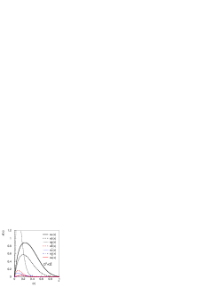
Figure 66: Probing (a) a valence parton in the proton and (b) a sea parton in a hadronic fluctuation (letters are four-momenta) resulting in (c) parton distributions at the starting scale $Q_{0}^{2}$.

The sea partons are obtained using a hadronic basis for the non-perturbative dynamics of the bound state proton and considering hadronic fluctuations

$$|p\rangle=\alpha_{0}|p_{0}\rangle+\alpha_{p\pi^{0}}|p\pi^{0}\rangle+\alpha_{n\pi^{+}}|n\pi^{+}\rangle+\ldots+\alpha_{\Lambda K}|\Lambda K^{+}\rangle+\ldots$$ (4.58)

Probing a parton $i$ in a hadron $H$ of a baryon-meson fluctuation $|BM\rangle$ (Fig. 66b) gives a sea parton with light-cone fraction $x=x_{H}\,x_{i}$ of the target proton. The momentum of the probed hadron is given by a similar Gaussian, but with a separate width parameter $\sigma_{H}$. Also here, kinematic constraints ensure physically allowed final states.

Using a Monte Carlo method the resulting valence and sea parton $x$-distributions are obtained without approximations. These apply at a low scale $Q_{0}^{2}$ and the distributions at higher $Q^{2}$ are obtained using perturbative QCD evolution at next-to-leading order. To describe all parton distributions (Fig. 66c), the model has only four shape parameters and three normalization parameters, plus the starting scale:

$$\begin{array}[]{c}\sigma_{u}=230\;\mathrm{MeV}\quad\sigma_{d}=170\;\mathrm{MeV}\quad\sigma_{g}=77\;\mathrm{MeV}\quad\sigma_{H}=100\;\mathrm{MeV}\\ \alpha_{\mathrm{p\pi^{0}}}^{2}=0.45\quad\alpha_{n\pi^{+}}^{2}=0.14\quad\alpha_{\Lambda K}^{2}=0.05\quad Q_{0}=0.75\;\mathrm{GeV}\end{array}$$ (4.59)

These are determined from fits to data as detailed in [166] and illustrated in Fig. 67. The model reproduces the inclusive proton structure function and gives a natural explanation of observed quark asymmetries, such as the difference between the up and down valence distributions and between the anti-up and anti-down sea quark distributions. Moreover, its asymmetry in the momentum distribution of strange and anti-strange quarks in the nucleon is large enough to reduce the NuTeV anomaly to a level which does not give a significant indication of physics beyong the Standard Model.

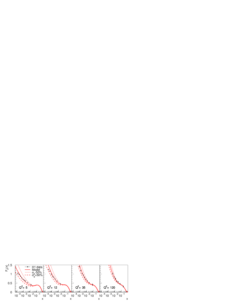
Figure 67: $F_{2}(x,Q^{2})$ from H1 compared to the model with $\pm 50\%$ variation of the width parameter $\sigma_{g}$ of the gluon distribution.

Recent fits of PDF’s at very low $x$ and $Q^{2}$ have revealed problems with the gluon density, which in some cases even becomes negative. The reason for this is that the DGLAP evolution, driven primarily by the gluon at small $x$, otherwise gives too large parton densities and thereby a poor fit to $F_{2}$ in the genuine DIS region at larger $Q^{2}$. It has been argued [168] that the root of the problem is the application of the formalism for DIS also in the low-$Q^{2}$ region, where the momentum transfer is not large enough that the parton structure of the proton is clearly resolved. The smallest distance that can be resolved is basically given by the momentum transfer of the exchanged photon through $d=0.2/\sqrt{Q^{2}}$, where $d$ is in Fermi if $Q^{2}$ is in GeV². This indicates that partons are resolved only for $Q^{2}\raisebox{-1.9919pt}{$\>\>\stackrel{{\scriptstyle>}}{{{\scriptstyle\sim}}}\>\>$}1\,\rm{GeV}^{2}$. For $Q^{2}\raisebox{-1.9919pt}{$\>\>\stackrel{{\scriptstyle<}}{{{\scriptstyle\sim}}}\>\>$}1\,\rm{GeV}^{2}$, there is no hard scale involved and a parton basis for the description is not justified. Instead, the interaction is here of a soft kind between the nearly on-shell photon and the proton. The cross section is then dominated by the process where the photon fluctuates into a virtual vector meson state which then interacts with the proton in a strong interaction. The quantum state of the photon can be expressed as $|\gamma\rangle=C_{0}|\gamma_{0}\rangle+\sum_{V}\frac{e}{f_{V}}|V\rangle+\int_{m_{0}}dm(\cdots)$. The sum is over $V=\rho^{0},\omega,\phi\ldots$ as in the original vector meson dominance model (VDM), whereas the generalised vector meson dominance model (GVDM) also includes the integral over a continuous mass spectrum (not written out explicitly here).

Applied to $ep$ at low $Q^{2}$ this leads to the expression [168]

$$F_{2}(x,Q^{2}) = \frac{(1-x)Q^{2}}{4\pi^{2}\alpha}\left\{\sum_{V=\rho,\omega,\phi}r_{V}\left(\frac{m_{V}^{2}}{Q^{2}+m_{V}^{2}}\right)^{2}\left(1+\xi_{V}\frac{Q^{2}}{m_{V}^{2}}\right)\right.$$ (4.60)

$$\left.+\;r_{C}\left[(1-\xi_{C})\frac{m_{0}^{2}}{Q^{2}+m_{0}^{2}}+\xi_{C}\frac{m_{0}^{2}}{Q^{2}}\ln{(1+\frac{Q^{2}}{m_{0}^{2}})}\right]\right\}A_{\gamma}\frac{Q^{2\epsilon}}{x^{\epsilon}}$$

where the hadronic cross-section $\sigma(ip\rightarrow X)=A_{i}s^{\epsilon}+B_{i}s^{-\eta}\approx A_{i}s^{\epsilon}\approx A_{i}(Q^{2}/x)^{\epsilon}$ has been used for the small-$x$ region of interest. The parameters involved are all essentially known from GVDM phenomenology. With $\epsilon=0.091$, $\xi=0.34$, $m_{0}=1.5$ GeV and $A_{\gamma}=71\,\mu\rm{b}$, this GVDM model gives a good fit ($\chi^{2}/\rm{d.o.f.}=87/66=1.3$) as illustrated in Fig. 68. Using this model at very low $Q^{2}$ in combination with the normal parton density approach at larger $Q^{2}$ it is possible to obtain a good description of data over the full $Q^{2}$ range [168]. This involves, however, a phenomenological matching of these two approaches, since a theoretically well justified combination is an unsolved problem.

Neglecting the GVDM component when fitting PDF’s to data at small $Q^{2}$ may thus lead to an improper gluon distribution, which is not fully universal and therefore may give incorrect results when used for cross section calculations at LHC.

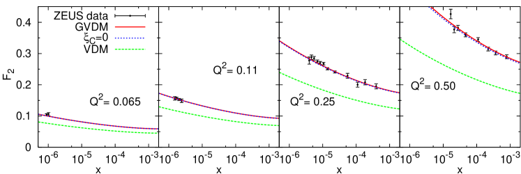
Figure 68: $F_{2}$ data at low $Q^{2}$ from ZEUS compared to the full GVDM in eq. (4.60) (full curves), when excluding the longitudinal contribution of the continuum ($\xi_{C}=0$) and excluding the continuous contribution altogether (setting $r_{C}=0$) giving VDM.

4.6 Towards precise determination of the nucleon PDFs

The nucleon parton distribution functions (PDFs) available to the moment are extracted from the rather limited set of experimental distributions (the deep-inelastic scattering (DIS) structure functions, the Drell-Yan (DY) and jet production cross sections). Other high-energy processes potentially could provide additional constraints on PDFs, however insufficient theoretical understanding does not allow to use those data without risk of having uncontrolled theoretical inaccuracies. Even for the case of the existing global fits of the PDFs performed by the MRST and CTEQ groups missing next-to-next-to-leading (NNLO) order QCD corrections to the Drell-Yan and jet production cross sections are not small as compared to the accuracy of the corresponding data used and therefore might give non-negligible effect. In this section we outline progress in the QCD fits with consistent account of the NNLO corrections.

4.6.1 Impact of the NNLO evolution kernel fixation on PDFs

In order to allow account of the NNLO corrections in the fit of PDFs one needs analytical expressions for the 3-loop corrections to the QCD evolution kernel. Until recent times these expressions were known only in the approximate form of Ref. [158] derived from the partial information about the kernel, including the set of its Mellin moments and the low-$x$ asymptotics [120, 121, 113] However with the refined calculations of Ref. [108, 109] the exact expression for the NNLO kernel has been available. These improvement is of particular importance for analysis of the low-$x$ data including the HERA ones due to general rise of the high-order QCD correction at low $x$. We illustrate impact of the NNLO evolution kernel validation on PDFs using the case of fit to the global DIS data [169, 170, 171, 172, 41, 54]. The exact NNLO corrections to the DIS coefficient functions are know [173, 106] that allowed to perform approximate NNLO fit of PDFs to these data [40] using the approximate NNLO corrections to the evolution kernel of Ref. [158]. Taking into account exact NNLO evolution kernel the analysis of Ref. [40] was updated recently to the exact NNLO case [174].

The gluon distributions at small $x$ obtained in these two variants of the fit are compared in Fig.69. With the exact NNLO corrections the QCD evolution of gluon distribution at small $x$ gets weaker and as a result at small $x/Q$ the gluon distribution obtained using the precise NNLO kernel is quite different from the approximate one. In particular, the approximate NNLO gluon distribution is negative at $Q^{2}\lesssim 1.3~{}{\rm GeV}^{2}$, while the precise one remains positive even below $Q^{2}=1~{}{\rm GeV}^{2}$. For the NLO case the positivity of gluons at small $x/Q$ is even worse than for the approximate NNLO case due to the approximate NNLO corrections dampen the gluon evolution at small $x$ too, therefore account of the NNLO corrections is crucial in this respect. (cf. discussion of Ref. [175]). Positivity of the PDFs is not mandatory beyond the QCD leading order, however it allows probabilistic interpretation of the parton model and facilitates modeling of the soft processes, such as underlying events in the hadron-hadron collisions at LHC. The change of gluon distribution at small $x/Q$ as compared to the fit with approximate NNLO evolution is rather due the change in evolution kernel than due to shift in the fitted parameters of PDFs. This is clear from comparison of the exact NNLO gluon distribution to one obtained from the approximate NNLO fit and evolved to low $Q$ using the exact NNLO kernel (see Fig.69). In the vicinity of crossover in the gluon distribution to the negative values its relative change due to variation of the evolution kernel is quite big and therefore further fixation of the kernel at small $x$ discussed in Ref. [176] might be substantial for validation of the PDFs at low $x/Q$. For the higher-mass kinematics at LHC numerical impact of the NNLO kernel update is not dramatic. Change in the Higgs and $W/Z$ bosons production cross sections due to more precise definition of the NNLO PDFs is comparable to the errors coming from the PDFs uncertainties, i.e. at the level of several percent.

Figure 69: The gluon distributions obtained in the different variants of PDFs fit to the DIS data (solid: the fit with exact NNLO evolution; dashes: the fit with approximate NNLO evolution; dots: the approximate NNLO gluons evolved with the exact NNLO kernel; dashed-dots: the NLO fit).

4.6.2 NNLO fit of PDFs to the combined DIS and Drell-Yan data

The DIS process provide very clean source of information about PDFs both from experimental and theoretical side, however very poorly constrains the gluon and sea distributions at $x\gtrsim 0.3$. The well known way to improve precision of the sea distributions is to combine DIS data with the Drell-Yan ones. The cross section of process $NN\rightarrow l^{+}l^{-}$ reads

$$\sigma_{DY}\propto\sum_{i}\left[q_{i}(x_{1})\bar{q}_{i}(x_{2})+q_{i}(x_{2})\bar{q}_{i}(x_{1})\right]+{\rm higher{{}^{{}_{\_}}}order~{}terms},$$

where $q(\bar{q})_{i}$ are the quarks(antiquarks) distribution and $x_{1,2}$ give the momentum fractions carried by each of the colliding partons. The quark distributions are determined by the DIS data with the precision of several percent in the wide region of $x$ and therefore precision of the sea distribution extracted from the combined fit to the DIS and DY data is basically determined by the latter. The Fermilab fixed-target experiments provide measurements of the DY cross sections for the isoscalar target [177] and the ratio of cross sections for the deuteron and proton targets [72] with the accuracy better than 20% at $x\lesssim 0.6$. Fitting PDFs to these data combined with the global DIS data of Ref. [169, 170, 171, 172, 41, 54] we can achieve comparable precision in the sea distributions. Recent calculations of Ref. [178] allow to perform this fit with full account of the NNLO correction. Using these calculations the DY data of Refs. [177, 72] were included into the NNLO fit of Ref. [174] that leads to significant improvement in the precision of sea distributions (see Fig. 70). Due to the DY data on the deuteron/proton ratio the isospin asymmetry of sea is also improved. It is worth to note that the precision achieved for the total sea distribution is in good agreement to the rough estimates given above. The value of $\chi^{2}/{\rm NDP}$ obtained in the fit is 1.1 and the spread of $\chi^{2}/{\rm NDP}$ over separate experiments used in the fit is not dramatic, its biggest value is 1.4. We rescaled the errors in data for experiments with $\chi^{2}/{\rm NDP}>1$ in order to bring $\chi^{2}/{\rm NDP}$ for this experiments to 1 and found that overall impact of this rescaling on the PDFs errors is marginal. This proofs sufficient statistical consistency of the data sets used in the fit and disfavors huge increase in the value of $\Delta\chi^{2}$ criterion suggested by the CTEQ collaboration for estimation of errors in the global fit of PDFs. A particular feature of the PDFs obtained is good stability with respect to the choice of factorization/renormalization scale in the DY cross section: Variation of this scale from $M_{\mu^{+}\mu^{-}}/2$ to $2M_{\mu^{+}\mu^{-}}$ leads to variation of PDFs comparable to their uncertainties due to errors in data.

Figure 70: Uncertainties in the non-strange sea distributions obtained from NNLO QCD fit to the DIS data combined with the fixed target Drell-Yan data (solid curves). The same uncertainties obtained in fit to the DIS data only [8] are given for comparison by dashes.

4.6.3 LHC data and flavor separation of the sea at small $x$

Combination of the existing DIS and fixed-target DY data provide good constraint on the total sea quarks distribution and allows separation of the $\bar{u}$- and $\bar{d}$-quark distributions up to the values of $x$ sufficient for most practical applications at the LHC. At small $x$ the total sea is also well constrained by the precise HERA data on the inclusive structure functions, however $\bar{u}/\bar{d}$ separation is poor in this region due to lack of the deuteron target data at HERA. The problem of the sea flavor separation is regularly masked due to additional constraints imposed on PDFs. In particular, most often the Regge-like behavior of the sea isospin asymmetry $x(\bar{d}-\bar{u})\propto x^{a_{ud}}$ is assumed with $a_{ud}$ selected around value of 0.5 motivated by the intercept of the meson trajectories. This assumption automatically provides constraint $\bar{d}=\bar{u}$ at $x\rightarrow 0$ and therefore leads to suppression of the uncertainties both in $\bar{u}$ and $\bar{d}$ at small $x$. If we do not assume the Regge-like behavior of $x(\bar{d}-\bar{u})$ its precision determined from the NNLO fit to the combined DIS and DY data of Section 1.2 is about 0.04 at $x=10^{-4}$ furthermore this constraint is defined rather by assumption about the shape of PDFs at small $x$ than by data used in the fit. The strange sea distribution is known much worse than the non-strange ones. It is essentially defined only by the CCFR experiment from the cross section of dimuon production in the neutrino nucleus collisions [179]. In this experiment the strange sea distribution was probed at $x=0.01\div 0.2$ and the shape obtained is similar to one of the non-strange sea with the strangeness suppression factor about 0.5. This is in clear disagreement with the Regge-like constraint on $x(\bar{d}-\bar{s})$ or $x(\bar{u}-\bar{s})$ and therefore we cannot use even this assumption to predict the strange sea at small $x$.

Figure 71: The $1\sigma$ error band for $x(\bar{d}-\bar{u})$ (upper panel) and $x(\bar{d}-\bar{s})$ (lower panel) expected for the fit of PDFs to the LHC data combined with the global DIS ones. Dashed curves correspond to the case of $Z/\gamma*$-production, dots are for the combination $Z/\gamma*$- with the $W^{+}/W^{-}$-production. Solid curves are for the central values obtained from the reference fit to the global DIS data

.

The LHC data on $\mu^{+}\mu^{-}$ production cross section can be used for further validation of the sea distributions at small $x$. Study of this process at the lepton pair masses down to 15 GeV will allow to probe PDFs at $x$ down to $10^{-4}$, while with both leptons detected full kinematics can be reliably reconstructed. In order to check impact of the foreseen LHC data on the sea flavor separation we generated sample of pseudo-data for the process $pp\rightarrow\mu^{+}\mu^{-}X$ at $\sqrt{s}=14~{}{\rm TeV}$ with integral luminosity of 10 1/fb corresponding to the first stage of the LHC operation. In order to meet typical limitations of the LHC detectors only events with the lepton pair absolute rapidity less than 2.5 were accepted; other detector effects were not taken into account. For generation of these pseudo-data we used PDFs obtained in the dedicated version of fit [174] with the sea distributions parameterized as $xS_{u,d,s}=\eta_{u,d,s}x^{a}(1-x)^{b_{u,d,s}}$ with the constraints $\eta_{u}=\eta_{d}=\eta_{s}$ and $b_{s}=(b_{u}+b_{d})/2$ imposed. These constraints are necessary for stability of the fit in view of limited impact of the DIS data on the flavor separation and, besides, the former one guarantees SU(3) symmetry in the sea distributions at small $x$. The generated pseudo-data were added to the basic DIS data sample and the errors in PDFs parameters were re-estimated with no constraints on the sea distributions imposed at this stage. Since dimuon data give extra information about the PDFs products they allow to disentangle the strange distribution, if an additional constraint on the non-strange sea distributions is set. The dashed curves in the lower panel of Fig.71 give the $1\sigma$ bands for $x(\bar{d}-\bar{s})$ as they are defined by the LHC simulated data combined with the global DIS ones given $(\bar{d}-\bar{u})$ is fixed. One can see that $\bar{d}/\bar{s}$ (and $\bar{u}/\bar{s}$) separation at the level of several percents would be feasible down to x=$10^{-4}$ in this case. The supplementary constraint on $(\bar{d}-\bar{u})$ can be obtained from study of the $W$-boson charge asymmetry. To estimate impact of this process we simulated the single $W^{+}$- and $W^{-}$-production data similarly to the case of the $\mu^{+}\mu^{-}$-production and took into account this sample too. In this case one can achieve separation of all three flavors with the precision better than 0.01 (see Fig.71). Note that strange sea separation is also improved due to certain sensitivity of the $W$-production cross section to the strange sea contribution. The estimates obtained refer to the ideal case of full kinematical reconstruction of the $W$-bosons events. For the case of using the charge asymmetry of muons produced from the $W$-decays the precision of the PDFs would be worse. Account of the backgrounds and the detector effects would also deteriorate it, however these losses can be at least partially compensated by rise of the LHC luminosity at the second stage of operation.

Valence	$a_{u}$	$0.718\pm 0.085$
	$b_{u}$	$3.81\pm 0.16$
	$\epsilon_{u}$	$-1.56\pm 0.46$
	$\gamma_{u}$	$3.30\pm 0.49$
	$a_{d}$	$1.71\pm 0.20$
	$b_{d}$	$10.00\pm 0.97$
	$\epsilon_{d}$	$-3.83\pm 0.23$
	$\gamma_{d}$	$4.64\pm 0.41$
Sea	$A_{S}$	$0.211\pm 0.016$
	$a_{s}$	$-0.048\pm 0.039$
	$b_{s}$	$2.20\pm 0.20$
Glue	$a_{G}$	$0.356\pm 0.095$
	$b_{G}$	$10.9\pm 1.4$
	$\alpha_{\rm s}(M_{\rm Z})$	$0.1132\pm 0.0015$

Table 19: Values of the parameters obtained in the benchmark fit.

4.6.4 Benchmarking of the PDFs fit

For the available nucleon PDFs the accuracy at percent level is reached in some kinematical regions. For this reason benchmarking of the codes used in these PDFs fits is becoming important issue. A tool for calibration of the QCD evolution codes was provided by Les Houches workshop [156]. To allow benchmarking of the PDFs errors calculation we performed a test fit suggested in Les Houches workshop too. This fit reproduces basic features of the existing global fits of PDFs, but is simplified a lot to facilitate its reproduction. We use for the analysis data on the proton DIS structure functions $F_{2}$ obtained by the BCDMS, NM, H1, and ZEUS collaborations and ratio of the deuteron and proton structure functions $F_{2}$ obtained by the NMC. The data tables with full description of experimental errors taken into account are available online. Cuts for the momentum transferred $Q^{2}>9~{}{\rm GeV}^{2}$ and for invariant mass of the hadronic system $W^{2}>15~{}{\rm GeV}^{2}$ are imposed in order to avoid influence of the power corrections and simplify calculations. The contribution of the $Z$-boson exchange at large $Q$ is not taken into account for the same purpose. The PDFs are parameterized in the form

$$xp_{i}(x,1~{}{GeV})=N_{i}x^{a_{i}}(1-x)^{b_{i}}(1+\epsilon_{i}\sqrt{x}+\gamma_{i}x),$$

to meet choice common for many popular global fits of PDFs. Some of the parameters $\epsilon_{i}$ and $\gamma_{i}$ are set to zero since they were found to be consistent to zero within the errors. We assume isotopic symmetry for sea distribution and the strange sea is the same as the non-strange ones suppressed by factor of 0.5. Evolution of the PDFs is performed in the NLO QCD approximation within the $\overline{\rm MS}$ scheme. The heavy quarks contribution is accounted in the massless scheme with the variable number of flavors (the thresholds for $c$- and $b$-quarks are 1.5 GeV and 4.5 GeV correspondingly). All experimental errors including correlated ones are taken into account for calculation of the errors in PDFs using the covariance matrix approach [180] and assuming linear propagation of errors. The results of the benchmark fit obtained with the code used in analysis of Refs.[40, 174] are given in Tables 19 and 20. The total number of the fitted PDF parameters left is 14. The normalization parameters $N_{i}$ for the gluon and valence quark distributions are calculated from the momentum and fermion number conservation. The remaining normalization parameter $A_{S}$ gives the total momentum carried by the sea distributions. Important note is that in view of many model assumptions made in the fit these results can be used mainly for the purposes of benchmarking rather for the phenomenological studies.

	$a_{u}$	$b_{u}$	$\epsilon_{u}$	$\gamma_{u}$	$a_{d}$	$b_{d}$	$\epsilon_{d}$	$\gamma_{d}$	$A_{S}$	$a_{s}$	$b_{s}$	$a_{G}$	$b_{G}$	$\alpha_{\rm s}(M_{\rm Z})$
$a_{u}$	1.000	0.728	-0.754	-0.708	0.763	0.696	-0.444	0.215	-0.216	-0.473	-0.686	0.593	0.777	-0.006
$b_{u}$	0.728	1.000	-0.956	-0.088	0.377	0.620	-0.420	0.387	0.175	-0.182	-0.713	0.067	0.505	-0.337
$\epsilon_{u}$	-0.754	-0.956	1.000	0.105	-0.388	-0.662	0.503	-0.485	-0.229	0.059	0.600	-0.047	-0.503	0.276
$\gamma_{u}$	-0.708	-0.088	0.105	1.000	-0.741	-0.390	0.219	0.107	0.597	0.591	0.310	-0.716	-0.675	-0.088
$a_{d}$	0.763	0.377	-0.388	-0.741	1.000	0.805	-0.622	0.248	-0.367	-0.509	-0.528	0.652	0.664	0.101
$b_{d}$	0.696	0.620	-0.662	-0.390	0.805	1.000	-0.904	0.728	0.017	-0.193	-0.512	0.272	0.576	-0.136
$\epsilon_{d}$	-0.444	-0.420	0.503	0.219	-0.622	-0.904	1.000	-0.896	-0.132	-0.019	0.245	-0.038	-0.362	0.173
$\gamma_{d}$	0.215	0.387	-0.485	0.107	0.248	0.728	-0.896	1.000	0.346	0.240	-0.107	-0.241	0.120	-0.228
$A_{S}$	-0.216	0.175	-0.229	0.597	-0.367	0.017	-0.132	0.346	1.000	0.708	0.127	-0.375	-0.026	0.047
$a_{s}$	-0.473	-0.182	0.059	0.591	-0.509	-0.193	-0.019	0.240	0.708	1.000	0.589	-0.595	-0.241	-0.011
$b_{s}$	-0.686	-0.713	0.600	0.310	-0.528	-0.512	0.245	-0.107	0.127	0.589	1.000	-0.508	-0.402	-0.109
$a_{G}$	0.593	0.067	-0.047	-0.716	0.652	0.272	-0.038	-0.241	-0.375	-0.595	-0.508	1.000	0.565	0.587
$b_{G}$	0.777	0.505	-0.503	-0.675	0.664	0.576	-0.362	0.120	-0.026	-0.241	-0.402	0.565	1.000	-0.138
$\alpha_{\rm s}(M_{\rm Z})$	-0.006	-0.337	0.276	-0.088	0.101	-0.136	0.173	-0.228	0.047	-0.011	-0.109	0.587	-0.138	1.000

Table 20: Correlation coefficients for the parameters obtained in the benchmark fit.

4.7 Benchmark Partons from DIS data and a Comparison with Global Fit Partons

In this article I consider the uncertainties on partons arising from the errors on the experimental data that are used in a parton analysis. Various groups [181],[182],[40],[18],[41], [34],[45] have concentrated on the experimental errors and have obtained estimates of the uncertainties on parton distributions within a NLO QCD framework, using a variety of competing procedures. Here the two analyses, performed by myself and S. Alekhin (see Sec. 4.6) minimise the differences one obtains for the central values of the partons and the size of the uncertainties by fitting to exactly the same data sets with the same cuts, and using the same theoretical prescription. In order to be conservative we use only DIS data – BCDMS proton [170] and deuterium [171] fixed target data, NMC data on proton DIS and on the ratio $F_{2}^{n}(x,Q^{2})/F_{2}^{p}(x,Q^{2})$ [172], and H1 [41] and ZEUS [54] DIS data. We also apply cuts of $Q^{2}=9{\rm GeV}^{2}$ and $W^{2}=15{\rm GeV}^{2}$ in order to avoid the influence of higher twist. We each use NLO perturbative QCD in the ${\overline{\rm MS}}$ renormalization and factorization scheme, with the zero-mass variable flavour number scheme and quark masses of $m_{c}=1.5{\rm GeV}$ and $m_{b}=4.5{\rm GeV}$. There is a very minor difference between $\alpha_{S}(\mu^{2})$ used in the two fitting programs due to the different methods of implementing heavy quark thresholds (the differences being formally of higher order), as observed in the study by M. Whalley for this workshop [184]. If the couplings in the two approaches have the same value at $\mu^{2}=M_{Z}^{2}$, then the MRST value is $\sim 1\%$ higher for $Q^{2}\sim 20{\rm GeV}^{2}$.

We each input our parton distributions at $Q_{0}^{2}=1{\rm GeV}^{2}$ with a parameterization of the form

$$xf_{i}(x,Q_{0}^{2})=A_{i}(1-x)^{b_{i}}(1+\epsilon_{i}x^{0.5}+\gamma_{i}x)x^{a_{i}}.$$ (4.61)

The input sea is constrained to be $40\%$ up and anti-up quarks, $40\%$ down and anti-down quarks, and $20\%$ strange and antistrange. No difference between $\bar{u}$ and $\bar{d}$ is input. There is no negative term for the gluon, as introduced in [34], since this restricted form of data shows no strong requirement for it in order to obtain the best fit. Similarly we are able to set $\epsilon_{g}$, $\gamma_{g}$, $\epsilon_{S}$ and $\gamma_{S}$ all equal to zero. $A_{g}$ is set by the momentum sum rule and $A_{u_{V}}$ and $A_{d_{V}}$ are set by valence quark number. Hence, there are nominally 13 free parton parameters. However, the MRST fitting program exhibited instability in the error matrix due to a very high correlation between $u_{V}$ parameters, so $\epsilon_{u}$ was set at its best fit value of $\epsilon_{u}=-1.56$, while 12 parameters were free to vary. The coupling was also allowed to vary in order to obtain the best fit. The treatment of the errors on the data was exactly as for the published partons with uncertainties for each group, i.e. as in [40] and [19]. This means that all detail on correlations between errors is included for the Alekhin fit (see Sec. 4.6), assuming that these errors are distributed in the Gaussian manner. The errors in the MRST fit are treated as explained in the appendix of [19], and the correlated errors are not allowed to move the central values of the data to as great an extent for the HERA data, and cannot do so at all for the fixed target data, where the data used are averaged over the different beam energies. The Alekhin approach is more statistically rigorous. The MRST approach is more pragmatic, reducing the ability of the data to move relative to the theory comparison by use of correlated errors (other than normalization), and is in some ways similar to the offset method [45]. The danger of this movement of data relative to theory has been suggested by the joint analysis of H1 and ZEUS data at this workshop (see Sec. 3.3), where letting the joint data sets determine the movement due to correlated errors gives different results from when the data sets are compared to theoretical results.

4.7.1 Comparison Between the Benchmark Parton Distributions.

I compare the results of the two approaches to fitting the restricted data chosen for the benchmarking. The input parameters for the Alekhin fit are presented in Sec. 4.6. Those for the MRST type fit are similar, but there are some differences which are best illustrated by comparing the partons at a typical $Q^{2}$ for the data, e.g. $Q^{2}=20{\rm GeV}^{2}$. A comparison is shown for the $d_{V}$ quarks and the gluon in Fig. 72.

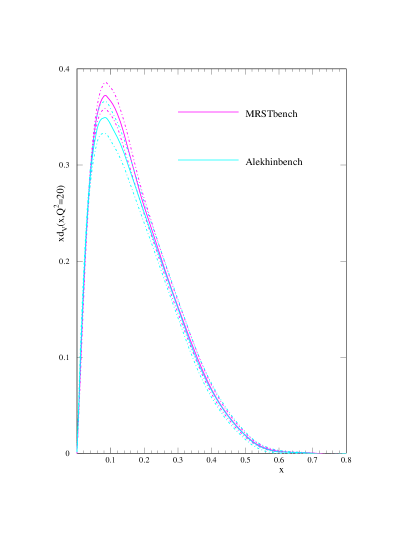
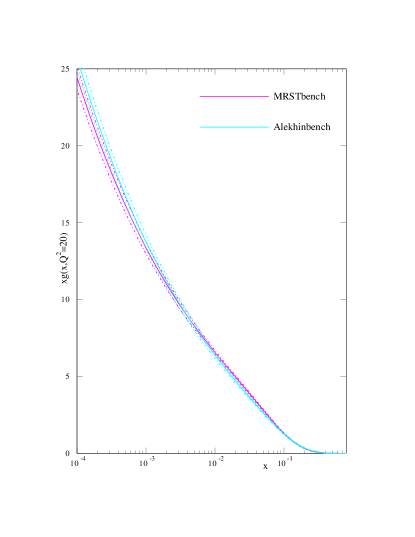
Figure 72: Left plot: $xd_{V}(x,20)$ from the MRST benchmark partons compared to that from the Alekhin benchmark partons. Right plot: $xg(x,20)$ from the MRST benchmark partons compared to that from the Alekhin benchmark partons.

From the plots it is clear that there is generally good agreement between the parton distributions. The central values are usually very close, and nearly always within the uncertainties. The difference in the central values is mainly due to the different treatment of correlated errors, and partially due to the difference in the coupling definition. The uncertainties are similar in the two sets, but are generally about $1.2-1.5$ times larger for the Alekhin partons, due to the increased freedom in the use of the correlated experimental errors. The values of $\alpha_{S}(M_{Z}^{2})$ are quite different, $\alpha_{S}(M_{Z}^{2})=0.1132\pm 0.0015$ compared to $0.1110\pm 0.0012$. However, as mentioned earlier, one expects a $1\%$ difference due to the different threshold prescriptions – the MRST $\alpha_{S}$ would be larger at $Q^{2}\sim 20{\rm GeV}^{2}$, where the data are concentrated, so correspondingly to fit the data it receives a $1\%$ shift downwards for $Q^{2}=M_{Z}^{2}$. Once this systematic effect is taken into account, the values of $\alpha_{S}(M_{Z}^{2})$ are very compatible. Hence, there is no surprising inconsistency between the two sets of parton distributions.

4.7.2 Comparison of the Benchmark Parton Distributions and Global Fit Partons.

It is also illuminating to show the comparison between the benchmark partons and the published partons from a global fit. This is done below for the MRST01 partons. For example, $u_{V}(x,Q^{2})$ and $\bar{u}(x,Q^{2})$ are shown in Fig. 73. It is striking that the uncertainties in the two sets are rather similar. This is despite the fact that the uncertainty on the benchmark partons is obtained from allowing $\Delta\chi^{2}=1$ in the fit while that for the MRST01 partons is obtained from $\Delta\chi^{2}=50$. This illustrates the great improvement in precision which is obtained due to the increase in data from the relaxation of the cuts and the inclusion of types of data other than DIS. For the $u_{V}$ partons, which are those most directly constrained by the DIS data in the benchmark fit, the comparison between the two sets of partons is reasonable, but hardly perfect – the central values differing by a few standard deviations. This is particularly important given that in this comparison the treatment of the data in the fit has been exactly the same in both cases. There is a minor difference in theoretical approach because of the simplistic treatment of heavy flavours in the benchmark fit. However, this would influence the gluon and sea quarks rather than valence quarks. Moreover, the region sensitive to this simplification would be $Q^{2}\sim m_{c}^{2}$ (the lower charge weighting for bottom quarks greatly reducing the effect near $Q^{2}=m_{b}^{2}$) which is removed by the $Q^{2}$ cut of $9{\rm GeV}^{2}$. Indeed, introducing the variable flavour number scheme usually used for the MRST partons modifies the benchmark partons only very minimally. Hence, if the statistical analysis is correct, the benchmark partons should agree with the global partons within their uncertainties (or at most 1.5 times their uncertainties, allowing for the effect of the correlated errors), which they do not. For the $\bar{u}$ partons the comparison is far worse, the benchmark partons being far larger at high $x$.

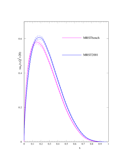
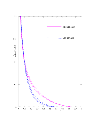
Figure 73: Left plot: $xu_{V}(x,20)$ from the MRST benchmark partons compared to that from the MRST01 partons. Right plot: $x\bar{u}(x,20)$ from the MRST benchmark partons compared to that from the MRST01 partons with emphasis on large $x$.

This disagreement in the high-$x$ $\bar{u}$ partons can be understood better if one also looks at the high-$x$ $d_{V}$ distribution shown in Fig. 74. Here the benchmark distribution is very much smaller than for MRST01. However, the increase in the sea distribution, which is common to protons and neutrons, at high-$x$ has allowed a good fit to the high-$x$ BCDMS deuterium data even with the very small high-$x$ $d_{V}$ distribution. In fact it is a better fit than in [19]. However, the fit can be shown to break down with the additional inclusion of high-$x$ SLAC data [169] on the deuterium structure function. More dramatically, the shape of the $\bar{u}$ is also completely incompatible with the Drell-Yan data usually included in the global fit, e.g. [177, 185]. Also in Fig. 74 we see that the $d_{V}$ distributions are very different at smaller $x$. The benchmark set is markedly inconsistent with NMC data on $F_{2}^{n}(x,Q^{2})/F_{2}^{p}(x,Q^{2})$ which is at small $x$, but below the cut of $Q^{2}=9{\rm GeV}^{2}$.

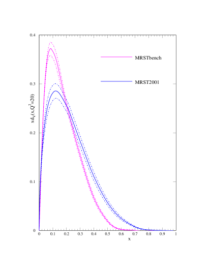
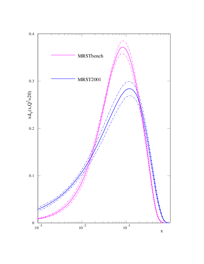
Figure 74: Left plot: $xd_{V}(x,20)$ from the MRST benchmark partons compared to that from the MRST01 partons. Right plot: $xd_{V}(x,20)$ from the MRST benchmark partons compared to that from the MRST01 partons with emphasis on small $x$.

The gluon from the benchmark set is also compared to the MRST01 gluon in Fig. 75. Again there is an enormous difference at high $x$. Nominally the benchmark gluon has little to constrain it at high $x$. However, the momentum sum rule determines it to be very small in this region in order to get the best fit to HERA data, similar to the gluon from [41]. As such, the gluon has a small uncertainty and is many standard deviations from the MRST01 gluon. Indeed, the input gluon at high $x$ is so small that its value at higher $Q^{2}$ is dominated by the evolution of $u_{V}$ quarks to gluons, rather than by the input gluon. Hence, the uncertainty is dominated by the quark parton input uncertainty rather than its own, and since the up quark is well determined the uncertainty on the high-$x$ gluon is small for the benchmark partons. The smallness of the high-$x$ gluon results in the benchmark partons producing a very poor prediction indeed for the Tevatron jet data [186, 187], which are the usual data that constrain the high-$x$ gluon in global fits.

It is also illustrative to look at small $x$. Here the benchmark gluon is only a couple of standard deviations from the MRST01 gluon, suggesting that its size is not completely incompatible with a good fit to the HERA small-$x$ data at $Q^{2}$ below the benchmark cut. However, the uncertainty in the benchmark gluon is much smaller than in the MRST01 gluon, despite the much smaller amount of low-$x$ data in the fit for the benchmark partons. This comes about as a result of the artificial choice made in the gluon input at $Q_{0}^{2}$. Since it does not have the term introduced in [19], allowing the freedom for the input gluon to be negative at very small $x$, the gluon is required by the fit to be valence-like. Hence, at input it is simply very small at small $x$. At higher $Q^{2}$ it becomes much larger, but in a manner driven entirely by evolution, i.e. it is determined by the input gluon at moderate $x$, which is well constrained. In this framework the small-$x$ gluon does not have any intrinsic uncertainty – its uncertainty is a reflection of moderate $x$. This is a feature of e.g. the CTEQ6 gluon uncertainty [18], where the input gluon is valence-like. In this case the percentage gluon uncertainty does not get any larger once $x$ reaches about $0.001$. The alternative treatment in [19] gives the expected increase in the gluon uncertainty as $x\to 0$, since in this case the uncertainty is determined largely by that in the input gluon at small $x$. The valence-like input form for a gluon is an example of fine-tuning, the form being unstable to evolution in either direction. The artificial limit on the small-$x$ uncertainty is a consequence of this.

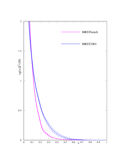
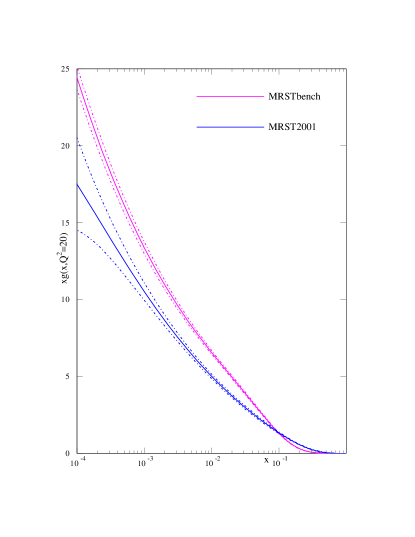
Figure 75: Left plot: $xg(x,20)$ from the MRST benchmark partons compared to that from the MRST2001 partons. Right plot: $xg(x,20)$ from the MRST benchmark partons compared to that from the MRST2001 partons with emphasis on small $x$.

4.7.3 Conclusions.

I have demonstrated that different approaches to fitting parton distributions that use exactly the same data and theoretical framework produce partons that are very similar and have comparable uncertainties. There are certainly some differences due to the alternative approaches to dealing with experimental errors, but these are relatively small. However, the partons extracted using a very limited data set are completely incompatible, even allowing for the uncertainties, with those obtained from a global fit with an identical treatment of errors and a minor difference in theoretical procedure. This implies that the inclusion of more data from a variety of different experiments moves the central values of the partons in a manner indicating either that the different experimental data are inconsistent with each other, or that the theoretical framework is inadequate for correctly describing the full range of data. To a certain extent both explanations are probably true. Some data sets are not entirely consistent with each other (even if they are seemingly equally reliable). Also, there are a wide variety of reasons why NLO perturbative QCD might require modification for some data sets, or in some kinematic regions [93]. Whatever the reason for the inconsistency between the MRST benchmark partons and the MRST01 partons, the comparison exhibits the dangers in extracting partons from a very limited set of data and taking them seriously. It also clearly illustrates the problems in determining the true uncertainty on parton distributions.

4.8 Stability of PDF fits

One of the issues raised at the workshop is the reliability of determinations of parton distribution functions (PDFs), which might be compromised for example by the neglect of NNLO effects or non-DGLAP evolution in the standard analysis, or hidden assumptions made in parameterizing the PDFs at nonperturbative scales. We summarize the results of the CTEQ PDF group on this issue. For the full story see [175].

4.8.1 Stability of PDF determinations

The stability of NLO global analysis was seriously challenged by an analysis [93] which found a 20% variation in the cross section predicted for $W$ production at the LHC – a critical “standard candle” process for hadron colliders – when certain cuts on input data are varied. If this instability were confirmed, it would significantly impact the phenomenology of a wide range of physical processes for the Tevatron Run II and the LHC. The CTEQ PDF group therefore performed an independent study of this issue within their global analysis framework. In addition, to explore the dependence of the results on assumptions about the parameterization of PDFs at the starting scale $Q_{0}\!=\!1.3\,\mathrm{GeV}$, we also studied the effect of allowing a negative gluon distribution at small $x$ – a possibility that is favored by the MRST NLO analysis, and that is closely tied to the W cross section controversy.

The stability of the global analysis was investigated by varying the inherent choices that must be made to perform the analysis. These choices include the selection of experimental data points based on kinematic cuts, the functional forms used to parameterize the initial nonperturbative parton distribution functions, and the treatment of $\alpha_{s}$.

The stability of the results is most conveniently measured by differences in the global $\chi^{2}$ for the relevant fits. To quantitatively define a change of $\chi^{2}$ that characterizes a significant change in the quality of the PDF fit is a difficult issue in global QCD analysis. In the context of the current analysis, we have argued that an increase by $\Delta\chi^{2}\sim 100$ (for $\sim$ ​ 2000 data points) represents roughly a 90% confidence level uncertainty on PDFs due to the uncertainties of the current input experimental data [188, 189, 190, 18]. In other words, PDFs with $\chi^{2}-\chi^{2}_{\mathrm{BestFit}}>100$ are regarded as not tolerated by current data.

The CTEQ6 and previous CTEQ global fits imposed “standard” cuts $Q>2\,\mathrm{GeV}$ and $W>3.5\,\mathrm{GeV}$ on the input data set, in order to suppress higher-order terms in the perturbative expansion and the effects of resummation and power-law (“higher twist”) corrections. We examined the effect of stronger cuts on $Q$ to see if the fits are stable. We also examined the effect of imposing cuts on $x$, which should serve to suppress any errors due to deviations from DGLAP evolution, such as those predicted by BFKL. The idea is that any inconsistency in the global fit due to data points near the boundary of the accepted region will be revealed by an improvement in the fit to the data that remain after those near-boundary points have been removed. In other words, the decrease in $\chi^{2}$ for the subset of data that is retained, when the PDF shape parameters are refitted to that subset alone, measures the degree to which the fit to that subset was distorted in the original fit by compromises imposed by the data at low $x$ and/or low $Q$.

The main results of this study are presented in Table 21. Three fits are shown, from three choices of the cuts on input data as specified in the table. They are labeled ‘standard’, ‘intermediate’ and ‘strong’. $N_{\rm pts}$ is the number of data points that pass the cuts in each case, and $\chi^{2}_{N_{\rm pts}}$ is the $\chi^{2}$ value for that subset of data. The fact that the changes in $\chi^{2}$ in each column are insignificant compared to the uncertainty tolerance is strong evidence that our NLO global fit results are very stable with respect to choices of kinematic cuts.

Cuts	$Q_{\mathrm{min}}$	$x_{\mathrm{min}}$	$N_{\mathrm{pts}}$	$\chi^{2}_{1926}$	$\chi^{2}_{1770}$	$\chi^{2}_{1588}$	$\sigma_{W}^{\mathrm{LHC}}\!\times\!B_{\ell\nu}\,[\mathrm{nb}]$
standard	$2\,\mathrm{GeV}$	$0$	$1926$	$2023$	$1850$	$1583$	$20.02$
intermediate	$2.5\,\mathrm{GeV}$	$0.001$	$1770$	–	$1849$	$1579$	$20.10$
strong	$3.162\,\mathrm{GeV}$	$0.005$	$1588$	–	–	$1573$	$20.34$

Table 21: Comparisons of three fits with different choices of the cuts on input data at the $Q$ and $x$ values indicated. In these fits, a conventional positive-definite gluon parameterization was used.

Cuts	$Q_{\mathrm{min}}$	$x_{\mathrm{min}}$	$N_{\mathrm{pts}}$	$\chi^{2}_{1926}$	$\chi^{2}_{1770}$	$\chi^{2}_{1588}$	$\sigma_{W}^{\mathrm{LHC}}\!\times\!B_{\ell\nu}\,[\mathrm{nb}]$
standard	$2\,\mathrm{GeV}$	$0$	$1926$	$2011$	$1845$	$1579$	$19.94$
intermediate	$2.5\,\mathrm{GeV}$	$0.001$	$1770$	–	$1838$	$1574$	$19.80$
strong	$3.162\,\mathrm{GeV}$	$0.005$	$1588$	–	–	$1570$	$19.15$

Table 22: Same as Table 21 except that the gluon parameterization is extended to allow negative values.

We extended the analysis to a series of fits in which the gluon distribution $g(x)$ is allowed to be negative at small $x$, at the scale $Q_{0}\!=\!1.3\,\mathrm{GeV}$ where we begin the DGLAP evolution. The purpose of this additional study is to determine whether the feature of a negative gluon PDF is a key element in the stability puzzle, as suggested by the findings of [93]. The results are presented in Table 22. Even in this extended case, we find no evidence of instability. For example, $\chi^{2}$ for the subset of 1588 points that pass the strong cuts increases only from 1570 to 1579 when the fit is extended to include the full standard data set.

Comparing the elements of Table 21 and Table 22 shows that our fits with $g(x)<0$ have slightly smaller values of$\chi^{2}$: e.g., $2011$ versus $2023$ for the standard cuts. However, the difference $\Delta\chi^{2}\!=\!12$ between these values is again not significant according to our tolerance criterion.

4.8.2 W cross sections at the LHC

The last columns of Tables 21 and 22 show the predicted cross section for $W^{+}+W^{-}$ production at the LHC. This prediction is also very stable: it changes by only $1.6\%$ for the positive-definite gluon parameterization, which is substantially less than the overall PDF uncertainty of $\sigma_{W}$ estimated previously with the standard cuts. For the negative gluon parameterization, the change is $4\%$–larger, but still less than the overall PDF uncertainty. These results are explicitly displayed, and compared to the MRST results in Fig. 76.

Figure 76: Predicted total cross section of $W^{+}+W^{-}$ production at the LHC for the fits obtained in our stability study, compared to the NLO results of Ref. [93]. The $Q$-cut values associated with the CTEQ points are given in the two tables. The overall PDF uncertainty of the prediction is $\sim 5\%$.

We see that this physical prediction is indeed insensitive to the kinematic cuts used for the fits, and to the assumption on the positive definiteness of the gluon distribution.

We also studied the stability of the prediction for $\sigma_{W}$ using the Lagrange Multiplier (LM) method of Refs. [188, 189, 190]. Specifically, we performed a series of fits to the global data set that are constrained to specific values of $\sigma_{W}$ close to the best-fit prediction. The resulting variation of $\chi^{2}$ versus $\sigma_{W}$ measures the uncertainty of the prediction. We repeated the constrained fits for each case of fitting choices (parameterization and kinematic cuts). In this way we gain an understanding of the stability of the uncertainty, in addition to the stability of the central prediction.

Figure 77 shows the results of the LM study for the three sets of kinematic cuts described in Table 21, all of which have a positive-definite gluon distribution.

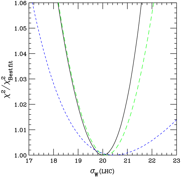
Figure 77: Lagrange multiplier results for the $W$ cross section (in $\mathrm{nb}$) at the LHC using a positive-definite gluon. The three curves, in order of decreasing steepness, correspond to the three sets of kinematic cuts labeled standard/intermediate/strong in Table 21.

The $\chi^{2}$ shown along the vertical axis is normalized to its value for the best fit in each series. In all three series, $\chi^{2}$ depends almost quadratically on $\sigma_{W}$. We observe several features:

• The location of the minimum of each curve represents the best-fit prediction for $\sigma_{W}^{\mathrm{LHC}}$ for the corresponding choice of cuts. The fact that the three minima are close together displays the stability of the predicted cross section already seen in Table 21.

• Although more restrictive cuts make the global fit less sensitive to possible contributions from resummation, power-law and other nonperturbative effects, the loss of constraints caused by the removal of precision HERA data points at small $x$ and low $Q$ results directly in increased uncertainties on the PDF parameters and their physical predictions. This is shown in Fig. 77 by the increase of the width of the curves with stronger cuts. The uncertainty of the predicted $\sigma_{W}$ increases by more than a factor of 2 in going from the standard cuts to the strong cuts.

Figure 78 shows the results of the LM study for the three sets of kinematic cuts described in Table 22, all of which have a gluon distribution which is allowed to go negative.

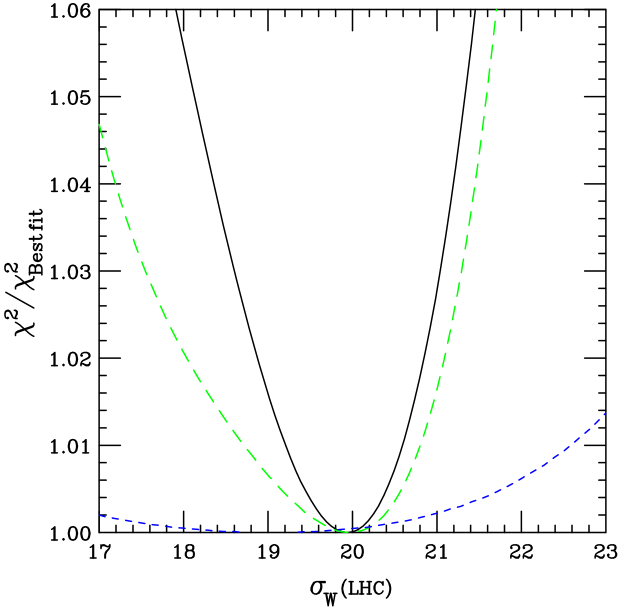
Figure 78: Lagrange multiplier results for the $W$ cross section (in $\mathrm{nb}$) at the LHC using a functional form where the gluon is not required to be positive-definite. The three curves, in order of decreasing steepness, correspond to the three sets of kinematic cuts labeled standard/intermediate/strong in Table 22.

We observe:

• Removing the positive definiteness condition necessarily lowers the value of $\chi^{2}$, because more possibilities are opened up in the $\chi^{2}$ minimization procedure. But the decrease is insignificant compared to other sources of uncertainty. Thus, a negative gluon PDF is allowed, but not required.

• The minima of the two curves occur at approximately the same $\sigma_{W}$. Allowing a negative gluon makes no significant change in the central prediction – merely a decrease of about $1\,\%$, which is small compared to the overall PDF uncertainty.

• For the standard set of cuts, allowing a negative gluon PDF would expand the uncertainty range only slightly. For the intermediate and strong cuts, allowing a negative gluon PDF would significantly expand the uncertainty range.

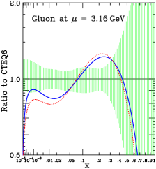
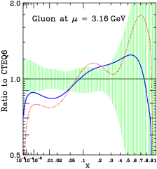
Figure 79: Left: mrst2002 NLO (solid) and NNLO (dotted); Right: mrst2004 NLO (solid) and NNLO (dotted); Shaded region is uncertainty according to the 40 eigenvector sets of CTEQ6.1.

We examined a number of aspects of our analysis that might account for the difference in conclusions between our stability study and that of [93]. A likely candidate seems to be that in order to obtain stability, it is necessary to allow a rather free parametrization of the input gluon distribution. This suspicion is seconded by recent work by MRST [191], in which a different gluon parametrization appears to lead to a best-fit gluon distribution that is close to that of CTEQ6. In summary, we found that the NLO PDFs and their physical predictions at the Tevatron and LHC are quite stable with respect to variations of the kinematic cuts and the PDF parametrization after all.

4.8.3 NLO and NNLO

In recent years, some preliminary next-to-next-leading-order (NNLO) analyses for PDFs have been carried out either for DIS alone [192], or in a global analysis context [39] – even if all the necessary hard cross sections, such as inclusive jet production, are not yet available at this order. Determining the parton distributions at NNLO is obviously desirable on theoretical grounds, and it is reasonable to plan for having a full set of tools for a true NNLO global analysis in place by the time LHC data taking begins. At the moment, however, NNLO fitting is not a matter of pressing necessity, since the difference between NLO and NNLO appears to be very small compared to the other uncertainties in the PDF analysis. This is demonstrated in Fig. 79, which shows the NLO and NNLO gluon distributions extracted by the MRST group. The difference between the two curves is much smaller than the other uncertainties measured by the 40 eigenvector uncertainty sets of CTEQ6.1, which is shown by the shaded region. The difference is also much smaller than the difference between CTEQ and MRST best fits. Similar conclusions [193] can be found using the NLO and NNLO fits by Alekhin.

4.9 The neural network approach to parton distributions

The requirements of precision physics at hadron colliders, as has been emphasized through this workshop, have recently led to a rapid improvement in the techniques for the determination of parton distribution functions (pdfs) of the nucleon. Specifically it is now mandatory to determine accurately the uncertainty on these quantities, and the different collaborations performing global pdf analysis[39, 194, 40] have performed estimations of these uncertainties using a variety of techniques. The main difficulty is that one is trying to determine the uncertainty on a function, that is, a probability measure in a space of functions, and to extract it from a finite set of experimental data, a problem which is mathematically ill-posed. It is also known that the standard approach to global parton fits have several shortcomings: the bias introduced by choosing fixed functional forms to parametrize the parton distributions (also known as model dependence), the problems to assess faithfully the pdf uncertainties, the combination of inconsistent experiments, and the lack of general, process-independent error propagation techniques. Although the problem of quantifying the uncertainties in pdfs has seen a huge progress since its paramount importance was raised some years ago, until now no unambiguous conclusions have been obtained.

In this contribution we present a novel strategy to address the problem of constructing unbiased parametrizations of parton distributions with a faithful estimation of their uncertainties, based on a combination of two techniques: Monte Carlo methods and neural networks. This strategy, introduced in [195, 196], has been first implemented to address the marginally simpler problem of parametrizing deep-inelastic structure functions $F(x,Q^{2})$, which we briefly summarize now. In a first step we construct a Monte Carlo sampling of the experimental data (generating artificial data replicas), and then we train neural networks to each data replica, to construct a probability measure in the space of structure functions $\mathcal{P}\left[F(x,Q^{2})\right]$. The probability measure constructed in this way contains all information from experimental data, including correlations, with the only assumption of smoothness. Expectation values and moments over this probability measure are then evaluated as averages over the trained network sample,

$$\left\langle\mathcal{F}\left[F(x,Q^{2})\right]\right\rangle=\int\mathcal{D}F\mathcal{P}\left[F(x,Q^{2})\right]\mathcal{F}\left[F(x,Q^{2})\right]=\frac{1}{N_{\mathrm{rep}}}\sum_{k=1}^{N_{\mathrm{rep}}}\mathcal{F}\left(F^{(\mathrm{net})(k)}(x,Q^{2})\right)\ .$$ (4.62)

where $\mathcal{F}\left[F\right]$ is an arbitrary function of $F(x,Q^{2})$.

The first step is the Monte Carlo sampling of experimental data, generating $N_{\mathrm{rep}}$ replicas of the original $N_{\mathrm{dat}}$ experimental data,

$$F_{i}^{(\mathrm{art})(k)}=\left(1+r_{N}^{(k)}\sigma_{N}\right)\left[F_{i}^{(\mathrm{exp})}+r_{i}^{s,(k)}\sigma^{stat}_{i}+\sum_{l=1}^{N_{sys}}r^{l,(k)}\sigma_{i}^{sys,l}\right],\qquad i=1,\ldots,N_{\mathrm{dat}}\ ,$$ (4.63)

where $r$ are gaussian random numbers with the same correlation as the respective uncertainties, and $\sigma^{stat},\sigma^{sys},\sigma_{N}$ are the statistical, systematic and normalization errors. The number of replicas $N_{\mathrm{rep}}$ has to be large enough so that the replica sample reproduces central values, errors and correlations of the experimental data.

The second step consists on training a neural network on each of the data replicas. Neural networks are specially suitable to parametrize parton distributions since they are unbiased, robust approximants and interpolate between data points with the only assumption of smoothness. The neural network training consist on the minimization for each replica of the $\chi^{2}$ defined with the inverse of the experimental covariance matrix,

$${\chi^{2}}^{(k)}=\frac{1}{N_{\mathrm{dat}}}\sum_{i,j=1}^{N_{\mathrm{dat}}}\left(F_{i}^{(\mathrm{art})(k)}-F_{i}^{(\mathrm{net})(k)}\right)\mathrm{cov}^{-1}_{ij}\left(F_{j}^{(\mathrm{art})(k)}-F_{j}^{(\mathrm{net})(k)}\right)\ .$$ (4.64)

Our minimization strategy is based on Genetic Algorithms (introduced in [197]), which are specially suited for finding global minima in highly nonlinear minimization problems.

The set of trained nets, once is validated through suitable statistical estimators, becomes the sought-for probability measure $\mathcal{P}\left[F(x,Q^{2})\right]$ in the space of structure functions. Now observables with errors and correlations can be computed from averages over this probability measure, using eq. (4.62). For example, the average and error of a structure function $F(x,Q^{2})$ at arbitrary $(x,Q^{2})$ can be computed as

$$\left\langle F(x,Q^{2})\right\rangle=\frac{1}{N_{\mathrm{rep}}}\sum_{k=1}^{N_{\mathrm{rep}}}F^{(\mathrm{net})(k)}(x,Q^{2}),\quad\sigma(x,Q^{2})=\sqrt{\left\langle F(x,Q^{2})^{2}\right\rangle-\left\langle F(x,Q^{2})\right\rangle^{2}}\ .$$ (4.65)

A more detailed account of the application of the neural network approach to structure functions can be found in [196], which describes the most recent NNPDF parametrization of the proton structure function.

Hence this strategy can be used also to parametrize parton distributions, provided one now takes into account perturbative QCD evolution. Therefore we need to define a suitable evolution formalism. Since complex neural networks are not allowed, we must use the convolution theorem to evolve parton distributions in $x-$space using the inverse $\Gamma(x)$ of the Mellin space evolution factor $\Gamma(N)$, defined as

$$q(N,Q^{2})=q(N,Q_{0}^{2})\Gamma\left(N,\alpha_{s}\left(Q^{2}\right),\alpha_{s}\left(Q_{0}^{2}\right)\right)\ ,$$ (4.66)

The only subtlety is that the x-space evolution factor $\Gamma(x)$ is a distribution, which must therefore be regulated at $x=1$, yielding the final evolution equation,

$$q(x,Q^{2})=q(x,Q_{0}^{2})\int_{x}^{1}dy~{}\Gamma(y)+\int_{x}^{1}\frac{dy}{y}\Gamma(y)\left(q\left(\frac{x}{y},Q_{0}^{2}\right)-yq(x,Q_{0}^{2})\right)\ ,$$ (4.67)

where in the above equation $q(x,Q_{0}^{2})$ is parametrized using a neural network. At higher orders in perturbation theory coefficient functions $C(N)$ are introduced through a modified evolution factor, $\tilde{\Gamma}(N)\equiv\Gamma(N)C(N)$. We have benchmarked our evolution code with the Les Houches benchmark tables [156] at NNLO up to an accuracy of $10^{-5}$. The evolution factor $\Gamma(x)$ and its integral are computed and interpolated before the neural network training in order to have a faster fitting procedure.

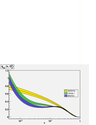
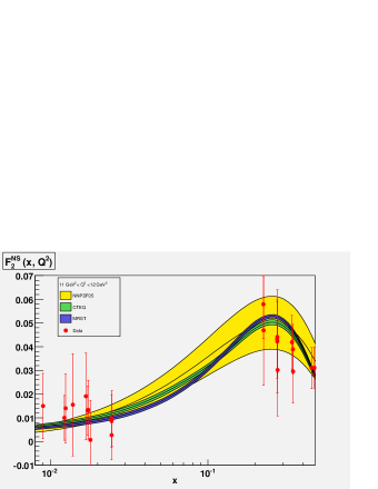
Figure 80: Preliminary results for the NNPDF $q_{NS}$ fit at $Q_{0}^{2}=2\,\mathrm{GeV}^{2}$, and the prediction for $F_{2}^{NS}(x,Q^{2})$ compared with the CTEQ and MRST results.

As a first application of our method, we have extracted the nonsinglet parton distribution $q_{NS}(x,Q^{2}_{0})=\frac{1}{6}\left(u+\bar{u}-d-\bar{d}\right)(x,Q^{2}_{0})$ from the nonsinglet structure function $F_{2}^{NS}(x,Q^{2})$ as measured by the NMC [172] and BCDMS [170, 171] collaborations. The preliminary results of a NLO fit with fully correlated uncertainties [198] can be seen in fig. 80 compared to other pdfs sets. Our preliminary results appear to point in the direction that the uncertainties at small $x$ do not allow, provided the current experimental data, to determine if $q_{NS}(x,Q^{2})$ grows at small $x$, as supported by different theoretical arguments as well as by other global parton fits. However, more work is still needed to confirm these results. Only additional nonsinglet structure function data at small $x$ could settle in a definitive way this issue.

Summarizing, we have described a general technique to parametrize experimental data in an bias-free way with a faithful estimation of their uncertainties, which has been successfully applied to structure functions and that now is being implemented in the context of parton distribution. The next step will be to construct a full set of parton distributions from all available hard-scattering data using the strategy described in this contribution.

5 Resummation^, 

5.1 Introduction

An accurate perturbative determination of the hard partonic cross-sections (coefficient functions) and of the anomalous dimensions which govern parton evolution is necessary for the precise extraction of parton densities. Recent progress in the determination of higher order contributions to these quantities has been reviewed in Sec. 4.2. As is well known, such high-order perturbative calculations display classes of terms containing large logarithms, which ultimately signal the breakdown of perturbation theory. Because these terms are scale–dependent and in general non universal, lack of their inclusion can lead to significant distortion of the parton densities in some kinematical regions, thereby leading to loss of accuracy if parton distributions extracted from deep-inelastic scattering (DIS) or the Drell-Yan (DY) processes are used at the LHC.

Logarithimic enhancement of higher order perturbative contribution may take place when more than one large scale ratio is present. In DIS and DY this happen in the two opposite limits when the center-of-mass energy of the partonic collision is much higher than the characteristic scale of the process, or close to the threshold for the production of the final state. These correspond respectively to the small $x$ and large $x$ kinematical regions, where $0\leq x\leq 1$ is defined in terms of the invariant mass $M^{2}$ of the non-leptonic final state as $M^{2}=\frac{(1-x)Q^{2}}{x}$. The corresponding perturbative contributions are respectively enhanced by powers of $\ln\frac{1}{x}$ and $\ln(1-x)$, or, equivalently, in the space of Mellin moments, by powers of $\frac{1}{N}$ and $\ln N$, where $N\to 0$ moments dominate as $x\to 0$ while $N\to\infty$ moments dominate as $x\to 1$.

The theoretical status of small $x$ and large $x$ resummation is somewhat different. Large $x$ logs are well understood and the corresponding perturbative corrections have been determined to all orders with very high accuracy. Indeed, the coefficients that determine their resummation can be extracted from fixed-order perturbative computations. Their resummation for DY and DIS was originally derived in [199, 200] and extended on very general grounds in [201]. The coefficients of the resulting exponentiation have now been determined so that resummation can now be performed exactly at ${\rm N}^{2}{\rm LL}$ [202, 108], and to a very good approximation at ${\rm N}^{3}{\rm LL}$ [203, 204, 205], including even some non-logarithmic terms [206]. On the other hand, small $x$ logs are due to the fact that at high energies, due to the opening of phase space, both collinear  [25, 24, 27] and high-energy [28, 29, 30, 207] logarithms contribute, and thus the coefficients required for their resummation can only be extracted from a simultaneous resolution of the DGLAP equation, which resums collinear logarithms, and the BFKL equation, which resum the high-energy logarithms. Although the determination of the kernels of these two equations has dramatically progressed in the last several years, thanks to the computation of the N²LO DGLAP kernel [108, 109] and of the NLO BFKL kernel [28, 29, 30, 207, 208, 209], the formalism which is needed to combine these two equations, as required for sucessful phenomenology, has only recently progressed to the point of being usable for realistic applications [210, 211, 212, 213, 214, 215, 176, 216, 217, 218].

In practice, however, neither small $x$ nor large $x$ resummation is systematically incorporated in current parton fits, so data points for which such effects may be important must be discarded. This is especially unsatisfactory in the case of large $x$ resummation, where resummed results (albeit with a varying degree of logarithmic accuracy) are available for essentially all processes of interest for a global parton fit, in particular, besides DIS and DY, prompt photon production [219, 220], jet production [221, 222] and heavy quark electroproduction [223, 224]. Even if one were to conclude that resummation is not needed, either because (at small $x$) it is affected by theoretical uncertainties or because (at large $x$) its effects are small, this conclusion could only be arrived at after a careful study of the impact of resummation on the determination of parton distributions, which is not available so far.

The purpose of this section is to provide a first assessment of the potential impact of the inclusion of small $x$ and large $x$ resummation on the determination of parton distributions. In the case of large $x$, this will be done by determining resummation effects on parton distributions extracted from structure functions within a simplified parton fit. In the case of small $x$, this will be done through a study of the impact of small $x$ resummation on splitting functions, as well as the theoretical uncertainty involved in the resummation process, in particular by comparing the results obtained within the approach of ref. [210, 211, 212] and that of ref. [213, 214, 215, 176, 216, 217, 218]. We will also discuss numerical approaches to the solution of the small-$x$ (BFKL) evolution equation.

5.2 Soft gluons

With the current level of theoretical control of soft gluon resummations, available calculations for DIS or DY should be fully reliable over most of the available phase space. Specifically, one expects current (resummed) predictions for DIS structure functions to apply so long as the leading power correction can be neglected, i.e. so long as $W^{2}\sim(1-x)Q^{2}>>\Lambda^{2}$, with $x=x_{Bj}$. Similarly, for the inclusive DY cross section, one would expect the same to be true so long as $(1-z)^{2}Q^{2}>>\Lambda^{2}$, where now $z=Q^{2}/\hat{s}$, with $\hat{s}=x_{1}x_{2}S$ the partonic center of mass energy squared. Indeed, as already mentioned, a consistent inclusion of resummation effects in parton fits is feasible with present knowledge: on the one hand, recent fits show that consistent parton sets can be obtained by making use of data from a single process (DIS) (see Sec. 3.3,4.6 and Ref. [174]), on the other hand, even if one adopts the philosophy of global fits, resummed calculations are available for all processes of interest.

In practice, however, currently available global parton fits are based on ${\rm NLO}$, or ${\rm N}^{2}{\rm LO}$ fixed-order perturbative calculations, so data points which would lie within the expected reach of resummed calculations cannot be fit consistently and must be discarded. The effect is that large-$x$ quark distributions become less constrained, which has consequences on the gluon distribution, as well as on medium-$x$ quark distributions, through sum rules and evolution. The pool of untapped information is growing, as more data at large values of $x$ have become available from, say, the NuTeV collaboration at Fermilab [225, 226]. A related issue is the fact that a growing number of QCD predictions for various processes of interest at the LHC are now computed including resummation effects in the hard partonic cross sections, which must be convoluted with parton densities in order to make predictions at hadron level. Such predictions are not fully consistent, since higher order effects are taken into account at parton level, but disregarded in defining the parton content of the colliding hadrons.

It is therefore worthwile to provide an assessment of the potential impact of resummation on parton distributions. Here, we will do this by computing resummation effects on quark distributions in the context of a simplified parton fit.

5.2.1 General Formalism in DIS

Deep Inelastic Scattering structure functions $F_{i}(x,Q^{2})$ are given by the convolution of perturbative coefficient functions, typically given in the $\overline{\mathrm{MS}}$ factorization scheme, and parton densities. The coefficient functions $C_{i}^{q}$ for quark-initiated DIS present terms that become large when the Bjorken variable $x$ for the partonic process is close to $x=1$, which forces gluon radiation from the incoming quark to be soft or collinear. At ${\cal O}(\alpha_{s})$, for example, the coefficient functions can be written in the form

$$C_{i}^{q}\left(x,\frac{Q^{2}}{\mu_{F}^{2}},\alpha_{s}(\mu^{2})\right)=\delta(1-x)+{\frac{\alpha_{s}(\mu^{2})}{2\pi}}H_{i}^{q}\left(x,\frac{Q^{2}}{\mu_{F}^{2}}\right)+{\cal O}\left(\alpha_{s}^{2}\right)\,.$$ (5.68)

Treating all quarks as massless, the part of $H_{i}^{q}$ which contains terms that are logarithmically enhanced as $x\to 1$ reads

$$H_{i,{\mathrm{soft}}}^{q}\left(x,\frac{Q^{2}}{\mu_{F}^{2}}\right)=2C_{F}\left\{\left[{\frac{\ln(1-x)}{1-x}}\right]_{+}+{\frac{1}{(1-x)_{+}}}\left(\frac{\ln Q^{2}}{\mu_{F}^{2}}-\frac{3}{4}\right)\right\}\,.$$ (5.69)

In moment space, where soft resummation is naturally performed, the contributions proportional to $\alpha_{s}[\ln(1-x)/(1-x)]_{+}$ and to $\alpha_{s}[1/(1-x)]_{+}$ correspond to double $(\alpha_{s}\ln^{2}N)$ and single $(\alpha_{s}\ln N)$ logarithms of the Mellin variable $N$. The Mellin transform of Eq. (5.69) in fact reads, at large $N$,

$$\hat{H}_{i,{\mathrm{soft}}}^{q}\left(N,\frac{Q^{2}}{\mu_{F}^{2}}\right)=2C_{F}\left\{{\frac{1}{2}}\ln^{2}N+\left[\gamma_{E}+{\frac{3}{4}}-\frac{\ln{Q^{2}}}{\mu_{F}^{2}}\right]\ln N\right\}\,.$$ (5.70)

All terms growing logarithmically with $N$, as well as all $N$-independent terms corresponding to contributions proportional to $\delta(1-x)$ in $x$-space, have been shown to exponentiate. In particular, the pattern of exponentiation of logarithmic singularities is nontrivial: one finds that the coefficient functions can be written as

$$\hat{C}_{i}^{q}\left(N,\frac{Q^{2}}{\mu_{F}^{2}},\alpha_{s}(\mu^{2})\right)={\cal R}\left(N,\frac{Q^{2}}{\mu_{F}^{2}},\alpha_{s}(\mu^{2})\right)\Delta\left(N,\frac{Q^{2}}{\mu_{F}^{2}},\alpha_{s}(\mu^{2})\right)\,,$$ (5.71)

where ${\cal R}(N,Q^{2}/\mu_{F}^{2},\alpha_{s}(\mu^{2}))$ is a finite remainder, nonsingular as $N\to\infty$, while [201]

$$\ln\Delta\left(N,\frac{Q^{2}}{\mu_{F}^{2}},\alpha_{s}(\mu^{2})\right)=\int_{0}^{1}{dx{\frac{{x^{N-1}-1}}{1-x}}}\left\{\int_{\mu_{F}^{2}}^{(1-x)Q^{2}}{\frac{dk^{2}}{k^{2}}}A\left[\alpha_{s}(k^{2})\right]+B\left[\alpha_{s}\left(Q^{2}(1-x)\right)\right]\right\}\,.$$ (5.72)

In Eq. (5.72) the leading logarithms (LL), of the form $\alpha^{n}_{s}\ln^{n+1}N$, are generated at each order by the function $A$. Next-to-leading logarithms (NLL), on the other hand, of the form $\alpha_{s}^{n}\ln^{n}N$, require the knowledge of the function $B$. In general, resumming ${\rm N}^{k}{\rm LL}$ to all orders requires the knowledge of the function $A$ to $k+1$ loops, and of the function $B$ to $k$ loops. In the following, we will adopt the common standard of NLL resummation, therefore we need the expansions

$$A(\alpha_{s})=\sum_{n=1}^{\infty}\left({\frac{\alpha_{s}}{\pi}}\right)^{n}A^{(n)}\ \ ;\ \ B(\alpha_{s})=\sum_{n=1}^{\infty}\left({\frac{\alpha_{s}}{\pi}}\right)^{n}B^{(n)}$$ (5.73)

to second order for $A$ and to first order for $B$. The relevant coefficients are

$$A^{(1)} = C_{F}\,,$$

$$A^{(2)} = {\frac{1}{2}}C_{F}\left[C_{A}\left({\frac{67}{18}}-{\frac{\pi^{2}}{6}}\right)-{\frac{5}{9}}n_{f}\right]\,,$$ (5.74)

$$B^{(1)} = -{\frac{3}{4}}C_{F}\,.$$

Notice that in Eq. (5.72) the term $\sim A(\alpha_{s}(k^{2}))/k^{2}$ resums the contributions of gluons that are both soft and collinear, and in fact the anomalous dimension $A$ can be extracted order by order from the residue of the singularity of the nonsinglet splitting function as $x\to 1$. The function $B$, on the other hand, is related to collinear emission from the final state current jet.

In [223, 224] soft resummation was extended to the case of heavy quark production in DIS. In the case of heavy quarks, the function $B(\alpha_{s})$ needs to be replaced by a different function, called $S(\alpha_{s})$ in [224], which is characteristic of processes with massive quarks, and includes effects of large-angle soft radiation. In the following, we shall consider values of $Q^{2}$ much larger than the quark masses and employ the resummation results in the massless approximation, as given in Eq. (5.72).

5.2.2 Simplified parton fit

We would like to use large-$x$ resummation in the DIS coefficient functions to extract resummed parton densities from DIS structure function data. Large-$x$ data typically come from fixed-target experiments: in the following, we shall consider recent charged-current (CC) data from neutrino-iron scattering, collected by the NuTeV collaboration [225, 226], and neutral-current (NC) data from the NMC [172] and BCDMS [170, 171] collaborations.

Our strategy will be to make use of data at different, fixed values of $Q^{2}$. We will extract from these data moments of the corresponding structure functions, with errors; since such moments factor into a product of moments of parton densities times moments of coefficient functions, computing parton moments with errors is straightforward. We then compare NLO to resummed partons in Mellin space, and subsequently provide a translation back to $x$-space by means of simple parametrization. Clearly, given the limited data set we are working with, our results will be affected by comparatively large errors, and we will have to make simplifying assumptions in order to isolate specific quark densities. Resummation effects are, however, clearly visible, and we believe that our fit provides a rough quantitative estimate of their size. A more precise quantitative analysis would have to be performed in the context of a global fit.

The first step is to construct a parametrization of the chosen data. An efficient and faithful parametrization of the NMC and BCDMS neutral-current structure functions was provided in [195, 196], where a large sample of Monte Carlo copies of the original data was generated, taking properly into account errors and correlations, and a neural network was trained on each copy of the data. One can then use the ensemble of networks as a faithful and unbiased representation of the probability distribution in the space of structure functions. We shall make use of the nonsinglet structure function $F_{2}^{\mathrm{ns}}(x,Q^{2})$ extracted from these data, as it is unaffected by gluon contributions, and provides a combination of up and down quark densities which is independent of the ones we extract from charged current data (specifically, $F_{2}^{\mathrm{ns}}(x,Q^{2})$ gives $u-d$).

As far as the NuTeV data are concerned, we shall consider the data on the CC structure functions $F_{2}$ and $F_{3}$. The structure function $F_{3}$ can be written as a convolution of the coefficient function $C_{3}^{q}$ with quark and antiquark distributions, with no gluon contribution, as

$$xF_{3}=\frac{1}{2}\left(xF_{3}^{\nu}+xF_{3}^{\bar{\nu}}\right)=x\left[\sum_{q,q^{\prime}}|V_{qq^{\prime}}|^{2}\left(q-\bar{q}\right)\otimes C_{3}^{q}\right].$$ (5.75)

We consider data for $F_{3}$ at $Q^{2}=12.59$ and $31.62$ GeV², and, in order to compute moments, we fit them using the functional form

$$xF_{3}(x)=Cx^{-\rho}(1-x)^{\sigma}(1+kx)~{}.$$ (5.76)

The best-fit values of $C$, $\rho$ and $\delta$, along with the $\chi^{2}$ per degree of freedom, are given in [227]. Here we show the relevant NuTeV data on $xF_{3}$, along with our best-fit curves, in Fig. 81.

Figure 81: NuTeV data on the structure function $xF_{3}$, at $Q^{2}=12.59~{}{\rm GeV}^{2}$ (a) and at $Q^{2}=31.62~{}{\rm GeV}^{2}$ (b), along with the best fit curve parametrized by Eq. (5.76).

The analysis of NuTeV data on $F_{2}$ is slightly complicated by the fact that gluon-initiated DIS gives a contribution, which, however, is not enhanced but suppressed at large $x$. We proceed therefore by taking the gluon density from a global fit, such as the NLO set CTEQ6M [18], and subtract from $F_{2}$ the gluon contribution point by point. We then write $F_{2}$ as

$$F_{2}\equiv\frac{1}{2}\left(F_{2}^{\nu}+F_{2}^{\bar{\nu}}\right)=x\sum_{q,q^{\prime}}|V_{qq^{\prime}}|^{2}\left[(q+\bar{q})\otimes C_{2}^{q}+g\otimes C_{2}^{g}\right]\equiv F_{2}^{q}+F_{2}^{g}\,,$$ (5.77)

and fit only the quark-initiated part $F_{2}^{q}$, using the same parametrization as in Eq. (5.76). Fig. 82 shows the data on $F_{2}^{q}$ and the best fit curves, as determined in Ref. [227].

Figure 82: NuTeV data on the quark-initiated contribution $F_{2}^{q}$ to the structure function $F_{2}$, for $Q^{2}=12.59~{}{\rm GeV}^{2}$ (a), and $Q^{2}=31.62~{}{\rm GeV}^{2}$ (b). The solid lines are the best-fit predictions.

After the subtraction of the gluon contribution from $F_{2}$, the structure functions we are considering ($F_{2}^{q}$, $xF_{3}$ and $F_{2}^{\mathrm{ns}}$) are all given in factorized form as

$$F_{i}(x,Q^{2})=x\int_{x}^{1}\frac{d\xi}{\xi}\,q_{i}\left(\xi,\mu_{F}^{2}\right)C_{i}^{q}\left(\frac{x}{\xi},\frac{Q^{2}}{\mu_{F}^{2}},\alpha_{s}(\mu^{2})\right)\,,$$ (5.78)

where $C_{i}^{q}$ is the relevant coefficient function and $q_{i}$ is a combination of quark and antiquark distributions only. Hereafter, we shall take $\mu=\mu_{F}=Q$ for the factorization and renormalization scales. At this point, to identify individual quark distributions from this limited set of data, we need to make some simplifying assumptions. Following [227], we assume isospin symmetry of the sea, $\bar{u}=\bar{d}$, $s=\bar{s}$ and we further impose a simple proportionality relation expressing the antistrange density in terms of the other antiquarks, $\bar{s}=\kappa\bar{u}$. As in [227], we shall present results for $\kappa=\frac{1}{2}$. With these assumptions, we can explicit solve for the remaining three independent quark densities (up, down, and, say, strange), using the three data sets we are considering.

Taking the Mellin moments of Eq. (5.78), the convolution becomes an ordinary product and we can extract NLO or NLL-resummed parton densities, according to whether we use NLO or NLL coefficient functions. More precisely,

$$\hat{q}_{i}^{\mathrm{NLO}}(N,Q^{2})=\frac{\hat{F}_{i}(N-1,Q^{2})}{\hat{C}_{i}^{\mathrm{NLO}}\left(N,1,\alpha_{s}(Q^{2})\right)}\,\,;\,\,\,\,\hat{q}_{i}^{\mathrm{res}}(N,Q^{2})=\frac{\hat{F}_{i}(N-1,Q^{2})}{\hat{C}_{i}^{\mathrm{res}}\left(N,1,\alpha_{s}(Q^{2})\right)}~{}.$$ (5.79)

After extracting the combinations $q_{i}$, one can derive the individual quark densities, at NLO and including NLL large-$x$ resummation. We concentrate our analysis on the up quark distribution, since experimental errors on the structure functions are too large to see an effect of the resummation on the other quark densities, such as $d$ or $s$, with the limited data set we are using.

5.2.3 Impact of the resummation

We present results for moments of the up quark distribution in Figs. 83 and 84.

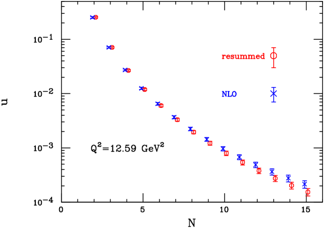
Figure 83: NLO and resummed moments of the up quark distribution at $Q^{2}=12.59$ GeV²

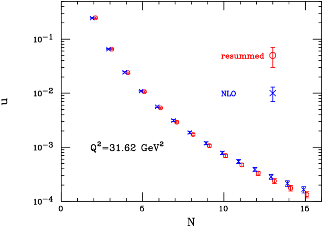
Figure 84: As in Fig. 83, but at $Q^{2}=31.62$ GeV².

Resummation effects become statistically significant around $N\sim 6-7$ at both values of $Q^{2}$. Notice that high moments of the resummed up density are suppressed with respect to the NLO density, as a consequence of the fact that resummation in the $\overline{\rm MS}\,\,$ scheme enhances high moments of the coefficient functions.

In order to illustrate the effect in the more conventional setting of $x$-space distributions, we fit our results for the moments to a simple parametrization of the form $u(x)=Dx^{-\gamma}(1-x)^{\delta}$. Our best fit values for the parameters, with statistical errors, are given in Table (23), and the resulting distributions are displayed in Fig. 85, with one standard deviation uncertainty bands.

$\hskip 8.53581ptQ^{2}$ PDF $\hskip 28.45274ptD$ $\hskip 28.45274pt\gamma$ $\hskip 5.69054pt\delta$ 12.59 NLO $3.025\pm 0.534$ $0.418\pm 0.101$ $3.162\pm 0.116$ RES $4.647\pm 0.881$ $0.247\pm 0.109$ $3.614\pm 0.128$ 31.62 NLO $2.865\pm 0.420$ $0.463\pm 0.086$ $3.301\pm 0.098$ RES $3.794\pm 0.583$ $0.351\pm 0.090$ $3.598\pm 0.104$

Table 23: Best fit values and errors for the up-quark $x$-space parametrization, at the chosen values of $Q^{2}$.

Once again, the effect of soft resummation is clearly visible at large $x$: it suppresses the quark densities extracted from the given structure function data with respect to the NLO prediction.

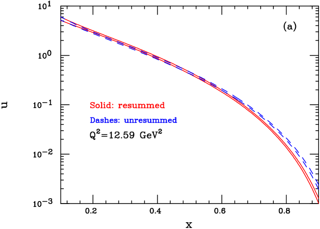
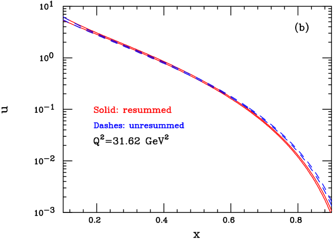
Figure 85: NLO and resummed up quark distribution at $Q^{2}=12.59$ GeV² (a) and at $Q^{2}=31.62$ GeV², using the parametrization given in the text. The band corresponds to one standard deviation in parameter space.

Figure 86: Central value for the relative change in the up quark distribution, $\Delta u(x)\equiv\left(u_{\rm NLO}(x)-u_{\rm res}(x)\right)/u_{\rm NLO}(x)$, at $Q^{2}=12.59$ (a) and 31.62 GeV² (b).

In order to present the effect more clearly, we show in Fig. 86 the normalized deviation of the NLL-resummed prediction from the NLO one, i.e. $\Delta u(x)=\left(u_{\rm NLO}(x)-u_{\rm res}(x)\right)/u_{\rm NLO}(x)$, at the two chosen values of $Q^{2}$ and for the central values of the best-fit parameters. We note a change in the sign of $\Delta u$ in the neighborhhod of the point $x=1/2$: although our errors are too large for the effect to be statistically significant, it is natural that the suppression of the quark distribution at large $x$ be compensated by an enhancement at smaller $x$. In fact, the first moment of the coefficient function is unaffected by the resummation: thus $C_{i}^{q}$, being larger at large $x$, must become smaller at small $x$. The further sign change at $x\sim 0.1$, on the other hand, should not be taken too seriously, since our sample includes essentially no data at smaller $x$, and of course we are using an $x$-space parametrization of limited flexibility.

Finally, we wish to verify that the up-quark distributions extracted by our fits at $Q^{2}=12.59$ and $31.62$ GeV² are consistent with perturbative evolution. To achieve this goal, we evolve our $N$-space results at $Q^{2}=31.62$ GeV² down to 12.59 GeV², using NLO Altarelli–Parisi anomalous dimensions, and compare the evolved moments with the direct fit at 12.59 GeV². Figures 87 and 88 show that the results of our fits at 12.59 GeV² are compatible with the NLO evolution within the confidence level of one standard deviation. Note however that the evolution of resummed moments appears to give less consistent results, albeit within error bands: this can probably be ascribed to a contamination between pertubative resummation and power corrections, which we have not disentangled in our analysis.

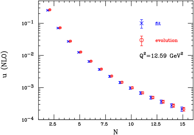
Figure 87: Comparison of fitted moments of the NLO up quark distribution, at $Q^{2}=12.59$ GeV², with moments obtained via NLO evolution from $Q^{2}=31.62$ GeV².

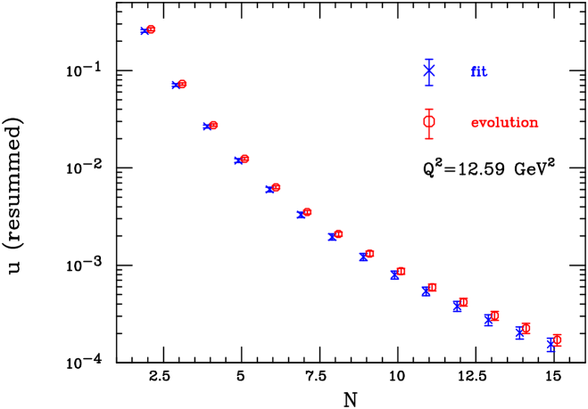
Figure 88: As in Fig. 87, but comparing NLL-resummed moments of the up quark density.

Qualitatively, the observed effect on the up quark distribution is easily described, at least within the limits of a simple parametrization like the one we are employing: resummation increases the exponent $\delta$, responsible for the power-law decay of the distribution at large $x$, by about $10\%$ to $15\%$ at moderate $Q^{2}$. The exponent $\gamma$, governing the small-$x$ behavior, and the normalization $D$, are then tuned so that the first finite moment (the momentum sum rule) may remain essentially unaffected.

In conclusion, our results indicate that quark distributions are suppressed at large $x$ by soft gluon effects. Quantitatively, we observe an effect ranging between $10\%$ and $20\%$ when $0.6<x<0.8$ at moderate $Q^{2}$, where we expect power corrections not to play a significant role. Clearly, a more detailed quantitative understanding of the effect can be achieved only in the context of a broader and fully consistent fit. We would like however to notice two things: first, the effect of resummations propagates to smaller values of $x$, through the fact that the momentum sum rule is essentially unaffected by the resummation; similarly, evolution to larger values of $Q^{2}$ will shift the Sudakov suppression to smaller $x$. A second point is that, in a fully consistent treatment of hadronic cross section, there might be a partial compensation between the typical Sudakov enhancement of the partonic process and the Sudakov suppression of the quark distribution: the compensation would, however, be channel-dependent, since gluon-initiated partonic processes would be unaffected. We believe it would be interesting, and phenomenologically relevant, to investigate these issues in the context of a more comprehensive parton fit.

5.3 Small $x$

Small $x$ structure functions are dominated by the flavour singlet contribution, whose coefficient functions and anomalous dimensions receive logarithmic enhancements, which make perturbation theory converge more slowly. In the small $x$, i.e. high energy limit, the cross section is quasi-constant and characterised by the effective expansion parameter $\langle\alpha_{s}(\boldsymbol{k}^{2})\rangle\log\frac{1}{x}\log\frac{\boldsymbol{k}_{\max}^{2}}{\boldsymbol{k}_{\min}^{2}}$, where $x=Q^{2}/s$, $\boldsymbol{k}^{2}\lesssim Q^{2}$ is the transverse momentum of the exchanged gluon, $s$ is the photon-proton centre of mass energy squared and $Q^{2}$ is the hard scale. Such expansion parameter can be large, due to both the double-logs and to the fact that $\langle\boldsymbol{k}^{2}\rangle$ may drift towards the non-perturbative region. Even assuming that truly non-perturbative effects are factored out — as is the case for structure functions — the problem remains of resumming the perturbative series with both kinds of logarithms [25, 24, 27, 28, 29, 30, 207]

In the BFKL approach one tries to resum the high-energy logarithms first, by an evolution equation in $\log 1/x$, whose $\boldsymbol{k}$-dependent evolution kernel is calculated perturbatively in $\alpha_{s}$. However, the leading kernel [28, 29, 30, 207] overestimates the hard cross-section, and subleading ones [114, 208, 209] turn out to be large and of alternating sign, pointing towards an instability of the leading-$\log x$ (L$x$) hierarchy. The problem is that, for any given value of the hard scales $Q,Q_{0}\ll\sqrt{s}$ — think, for definiteness, of $\gamma^{*}(Q)$-$\gamma^{*}(Q_{0})$ collisions —, the contributing kernels contain collinear enhancements in all $\boldsymbol{k}$-orderings of the exchanged gluons of type $\sqrt{s}\gg\cdots\boldsymbol{k}_{1}\gg\boldsymbol{k}_{2}\cdots$, or $\sqrt{s}\gg\cdots\boldsymbol{k}_{2}\gg\boldsymbol{k}_{1}\cdots$ and so on, to all orders in $\alpha_{s}$. Such enhancements are only partly taken into account by any given truncation of the L$x$ hierarchy, and they make it unstable. In the DGLAP evolution equation one resums collinear logarithms first, but fixed order splitting functions do contain [108, 109] high-energy logarithms also, and a further resummation is needed.

Two approaches to the simultaneous resummation of these two classes of logs have recently reached the stage where their phenomenological application can be envisaged. The renormalisation group improved (CCSS) approach [210, 211, 212, 228] is built up within the BFKL framework, by improving the whole hierarchy of subleading kernels in the collinear region, so as to take into account all the $\boldsymbol{k}$-orderings mentioned before, consistently with the RG. In the duality (ABF) approach [229, 213, 214, 215, 176, 216, 217, 218] one concentrates on the problem of obtaining an improved anomalous dimension (splitting function) for DIS which reduces to the ordinary perturbative result at large $N$ (large $x$), thereby automatically satisfying renormalization group constraints, while including resummed BFKL corrections at small $N$ (small $x$), determined through the renormalization-group improved (i.e. running coupling) version of the BFKL kernel.

We will briefly review the theoretical underpinnings of these two approaches in turn, and then compare phenomenological results obtained in both approaches. Note that we shall use the notation of the CCSS or ABF papers in the corresponding sections, in order to enable a simpler connection with the original literature, at the price of some notational discontinuity. In particular, $\ln\frac{1}{x}$ is called $Y$ by CCSS and $\xi$ by ABF; the Mellin variable conjugate to $\ln\frac{1}{x}$ is called $\omega$ by CCSS and $N$ by ABF; and the Mellin variable conjugated to $\ln\frac{Q^{2}}{{\boldsymbol{k}}^{2}}$ is called $\gamma$ by CCSS and $M$ by ABF.

5.3.1 The renormalisation group improved approach

The basic problem which is tackled in the CCSS approach [210, 211, 212, 228] is the calculation of the (azimuthally averaged) gluon Green function ${\cal G}(Y;k,k_{0})$ as a function of the magnitudes of the external gluon transverse momenta $k\equiv|\boldsymbol{k}|,\;k_{0}\equiv|\boldsymbol{k}_{0}|$ and of the rapidity $Y\equiv\log\frac{s}{kk_{0}}$. This is not yet a hard cross section, because one needs to incorporate the impact factors of the probes [230, 231, 232, 233, 234, 235, 236, 237]. Nevertheless, the Green function exhibits most of the physical features of the hard process, if we think of $k^{2},\;k_{0}^{2}$ as external (hard) scales. The limits $k^{2}\gg k_{0}^{2}$ ($k_{0}^{2}\gg k^{2}$) correspond conventionally to the ordered (anti-ordered) collinear limit. By definition, in the $\omega$-space conjugate to $Y$ (so that $\hat{\omega}=\partial_{Y}$) one sets

$${\cal G}_{\omega}(\boldsymbol{k},\boldsymbol{k}_{0}) \equiv[\omega-{\cal K}_{\omega}]^{-1}(\boldsymbol{k},\boldsymbol{k}_{0})\,,$$ (5.80)

$$\omega{\cal G}_{\omega}(\boldsymbol{k},\boldsymbol{k}_{0}) =\delta^{2}(\boldsymbol{k}-\boldsymbol{k}_{0})+\int d^{2}\boldsymbol{k}^{\prime}\;{\cal K}_{\omega}(\boldsymbol{k},\boldsymbol{k}^{\prime}){\cal G}_{\omega}(\boldsymbol{k}^{\prime},\boldsymbol{k}_{0})\;,$$ (5.81)

where ${\cal K}_{\omega}(\boldsymbol{k},\boldsymbol{k}^{\prime})$ is a kernel to be defined, whose $\omega=0$ limit is related to the BFKL $Y$-evolution kernel discussed before.

In order to understand the RG constraints, it is useful to switch from $\boldsymbol{k}$-space to $\gamma$-space, where the variable $\gamma$ is conjugated to $t\equiv\log\boldsymbol{k}^{2}/\boldsymbol{k}_{0}^{2}$ at fixed $Y$, and to make the following kinematical remark: the ordered (anti-ordered) region builds up scaling violations in the Bjorken variable $x=\boldsymbol{k}^{2}/s$ ($x_{0}=\boldsymbol{k}_{0}^{2}/s$) and, if $x$ ($x_{0}$) is fixed instead of $kk_{0}/s=e^{-Y}$, the variable conjugated to $t$ is shifted [238] by an $\omega$-dependent amount, and becomes $\gamma+{\textstyle\frac{\omega}{2}}\sim\partial_{\log\boldsymbol{k}^{2}}$   ($1-\gamma+{\textstyle\frac{\omega}{2}}\sim\partial_{\log\boldsymbol{k}_{0}^{2}}$). Therefore, the characteristic function $\chi_{\omega}(\gamma)$ of ${\cal K}_{\omega}$ (with a factor $\alpha_{s}$ factored out) must be singular when either one of the variables is small, as shown (in the frozen $\alpha_{s}$ limit) by

$$\frac{1}{\omega}\chi_{\omega}(\gamma)\to\left[\frac{1}{\gamma+{\textstyle\frac{\omega}{2}}}+\frac{1}{1-\gamma+{\textstyle\frac{\omega}{2}}}+\cdots\right]\left[\gamma_{gg}^{(1)}(\alpha_{s},\omega)+\cdots\right]\;,$$ (5.82)

where $\gamma_{gg}^{(1)}$ is the one-loop gluon anomalous dimension, and further orders may be added. Eq. (5.82) ensures the correct DGLAP evolution in either one of the collinear limits (because, e.g., $\gamma+{\textstyle\frac{\omega}{2}}\sim\partial_{\log\boldsymbol{k}^{2}}$) and is $\omega$-dependent, because of the shifts. Since higher powers of $\omega$ are related to higher subleading powers of $\alpha_{s}$ [239], this $\omega$-dependence of the constraint (5.82) means that the whole hierarchy of subleading kernels is affected.

To sum up, the kernel ${\cal K}_{\omega}$ is constructed so as to satisfy the RG constraint (5.82) and to reduce to the exact L$x$ + NL$x$ BFKL kernels in the $\omega\to 0$ limit; it is otherwise interpolated on the basis of various criteria (e.g., momentum conservation), which involve a “scheme” choice.

The resulting integral equation has been solved in [210, 211, 212] by numerical matrix evolution methods in $\boldsymbol{k}$- and $x$-space. Furthermore, introducing the integrated gluon density $g$, the resummed splitting function $P_{\mathrm{eff}}(x,Q^{2})$ is defined by the evolution equation

$$\frac{\partial g(x,Q^{2})}{\partial\log Q^{2}}=\int\frac{\mathrm{d}z}{z}\;P_{\mathrm{eff}}\big{(}z,\alpha_{s}(Q^{2})\big{)}g\Big{(}\frac{x}{z},Q^{2}\Big{)}\;,$$ (5.83)

and has been extracted [210, 211, 212] by a numerical deconvolution method [240]. Note that in the RGI approach the running of the coupling is treated by adopting in (5.81) the off-shell dependence of $\alpha_{s}$ suggested by the BFKL and DGLAP limits, and then solving the ensuing integral equation numerically.

It should be noted that the RGI approach has the somewhat wider goal of calculating the off-shell gluon density (5.80), not only its splitting function. Therefore, a comparison with the ABF approach, to be discussed below, is possible in the “on-shell” limit, in which the homogeneous (eigenvalue) equation of RGI holds. In the frozen coupling limit we have simply

$$\chi_{\omega}(\alpha_{s},\gamma-{\textstyle\frac{\omega}{2}})=\omega\;,\qquad(\text{$\chi_{\omega}$ is at scale $kk_{0}$})\;.$$ (5.84)

Solving Eq. (5.84) for either $\omega$ or $\gamma$, we are able to identify the effective characteristic function and its dual anomalous dimension

$$\omega=\chi_{\mathrm{eff}}(\alpha_{s},\gamma)\;;\quad\gamma=\gamma_{\mathrm{eff}}(\alpha_{s},\omega)\;,$$ (5.85)

in the same spirit as the ABF approach [229, 213, 214, 215, 176, 216, 217, 218].

5.3.2 The duality approach

As already mentioned, in the ABF approach one constructs an improved anomalous dimension (splitting function) for DIS which reduces to the ordinary perturbative result at large $N$ (large $x$) given by:

$$\gamma(N,\alpha_{s})=\alpha_{s}\gamma_{0}(N)~{}+~{}\alpha_{s}^{2}\gamma_{1}(N)~{}+~{}\alpha_{s}^{3}\gamma_{2}(N)~{}~{}\dots.$$ (5.86)

while including resummed BFKL corrections at small $N$ (small $x$) which are determined by the aforementioned BFKL kernel $\chi(M,\alpha_{s})$:

$$\chi(M,\alpha_{s})=\alpha_{s}\chi_{0}(M)~{}+~{}\alpha_{s}^{2}\chi_{1}(M)~{}+~{}\dots,$$ (5.87)

which is the Mellin transform of the $\omega\to 0$, angular averaged kernel ${\cal K}$ eq. 5.81 with respect to $t=\ln\frac{k^{2}}{k_{0}^{2}}$. The main theoretical tool which enables this construction is the duality relation between the kernels $\chi$ and $\gamma$

$$\chi(\gamma(N,\alpha_{s}),\alpha_{s})=N,$$ (5.88)

[compare eq. (5.85)] which is a consequence of the fact that the solutions of the BFKL and DGLAP equations coincide at leading twist [241, 229, 213]. Further improvements are obtained exploiting the symmetry under gluon interchange of the BFKL gluon-gluon kernel and through the inclusion of running coupling effecs.

By using duality, one can construct a more balanced expansion for both $\gamma$ and $\chi$, the ”double leading” (DL) expansion, where the information from $\chi$ is used to include in $\gamma$ all powers of $\alpha_{s}/N$ and, conversely $\gamma$ is used to improve $\chi$ by all powers of $\alpha_{s}/M$. A great advantage of the DL expansion is that it resums the collinear poles of $\chi$ at $M=0$, enabling the imposition of the physical requirement of momentum conservation $\gamma(1,\alpha_{s})=0$, whence, by duality:

$$\chi(0,\alpha_{s})=1.$$ (5.89)

This procedure eliminates in a model independent way the alternating sign poles $+1/M,-1/M^{2},.....$ that appear in $\chi_{0}$, $\chi_{1}$,…. These poles make the perturbative expansion of $\chi$ unreliable even in the central region of $M$: e.g., $\alpha_{s}\chi_{0}$ has a minimum at $M=1/2$, while, at realistic values of $\alpha_{s}$, $\alpha_{s}\chi_{0}+\alpha_{s}^{2}\chi_{1}$ has a maximum.

At this stage, while the poles at $M=0$ are eliminated, those at $M=1$ remain, so that the DL expansion is still not finite near $M=1$. The resummation of the $M=1$ poles can be accomplished by exploiting the collinear-anticollinear symmetry, as suggested in the CCSS approach discussed above. In Mellin space, this symmetry implies that at the fixed-coupling level the kernel $\chi$ for evolution in $\ln\frac{s}{kk_{0}}$ must satisfy $\chi(M)=\chi(1-M)$. This symmetry is however broken by the DIS choice of variables $\ln\frac{1}{x}=\ln\frac{s}{Q^{2}}$ and by the running of the coupling. In the fixed coupling limit the kernel $\chi_{\rm DIS}$, dual to the DIS anomalous dimension, is related to the symmetric one $\chi_{\sigma}$ through the implicit equation [114]

$$\chi_{\rm DIS}(M+1/2\chi_{\rm\sigma}(M))=\chi_{\sigma}(M),$$ (5.90)

to be compared to eq. (5.84) of the CCSS approach.

Hence, the $M=1$ poles can be resummed by performing the double-leading resummation of $M=0$ poles of $\chi_{\rm DIS}$, determining the associated $\chi_{\sigma}$ through eq. (5.90), then symmetrizing it, and finally going back to DIS variables by using eq. (5.90) again in reverse. Using the momentum conservation eq. (5.89) and eq. (5.90), it is easy to show that $\chi_{\sigma}(M)$ is an entire function of M, with $\chi_{\sigma}(-1/2)=\chi_{\sigma}(3/2)=1$ and has a minimum at $M=1/2$. Through this procedure one obtains order by order from the DL expansion a symmetrized DL kernel $\chi_{\rm DIS}$, and its corresponding dual anomalous dimension $\gamma$. The kernel $\chi_{\rm DIS}$ has to all orders a minimum and satisfies a momentum conservation constraint $\chi_{\rm DIS}(0)=\chi_{\rm DIS}(2)=1$.

The final ingredient of the ABF approach is a treatment of the running coupling corrections to the resummed terms. Indeed, their inclusion in the resummed anomalous dimension greatly softens the asymptotic behavior near $x=0$. Hence, the dramatic rise of structure functions at small $x$, which characterized resummations based on leading–order BFKL evolution, and is ruled out phenomenologically, is replaced by a much milder rise. This requires a running coupling generalization of the duality equation (5.88), which is possible noting that in $M$ space the running coupling $\alpha_{s}(t)$ becomes a differential operator, since $t\rightarrow d/dM$. Hence, the BFKL evolution equation for double moments $G(N,M)$, which is an algebraic equation at fixed coupling, becomes a differential equation in $M$ for running coupling. In the ABF approach, one solves this differential equation analytically when the kernel is replaced by its quadratic approximation near the minimum. The solution is expressed in terms of an Airy function if the kernel is linear in $\alpha_{s}$, for example in the case of $\alpha_{s}\chi_{0}$, or of a Bateman function in the more general case of a non linear dependence on $\alpha_{s}$ as is the case for the DL kernels. The final result for the improved anomalous dimension is given in terms of the DL expansion plus the “Airy” or “Bateman” anomalous dimension, with the terms already included in the DL expansion subtracted away.

For example, at leading DL order, i.e. only using $\gamma_{0}(N)$ and $\chi_{0}(M)$, the improved anomalous dimension is

$$\gamma_{I}^{NL}(\alpha_{s},N)=\Big{[}\alpha_{s}\gamma_{0}(N)+\alpha_{s}^{2}\gamma_{1}(N)+\gamma_{s}(\frac{\alpha_{s}}{N})-\frac{n_{c}\alpha_{s}}{\pi N}\Big{]}+\gamma_{A}(c_{0},\alpha_{s},N)-\frac{1}{2}+\sqrt{\frac{2}{\kappa_{0}\alpha_{s}}[N-\alpha_{s}c_{0}]}.$$ (5.91)

The terms within square brackets give the LO DL approximation, i.e. they contain the fixed–coupling information from $\gamma_{0}$ and (through $\gamma_{s}$) from $\chi_{0}$. The “Airy” anomalous dimension $\gamma_{A}(c_{0},\alpha_{s},N)$ contains the running coupling resummation, i.e. it is the exact solution of the running coupling BFKL equation which corresponds to a quadratic approximation to $\chi_{0}$ near $M=1/2$. The last two terms subtract the contributions to $\gamma_{A}(c_{0},\alpha_{s},N)$ which are already included in $\gamma_{s}$ and $\gamma_{0}$. In the limit $\alpha_{s}\rightarrow 0$ with $N$ fixed, $\gamma_{I}(\alpha_{s},N)$ reduces to $\alpha_{s}\gamma_{0}(N)+O(\alpha_{s}^{2})$. For $\alpha_{s}\rightarrow 0$ with $\alpha_{s}/N$ fixed, $\gamma_{I}(\alpha_{s},N)$ reduces to $\gamma_{s}(\frac{\alpha_{s}}{N})+O(\alpha_{s}^{2}/N)$, i.e. the leading term of the small $x$ expansion. Thus the Airy term is subleading in both limits. However, if $N\to 0$ at fixed $\alpha_{s}$, the Airy term replaces the leading singularity of the DL anomalous dimension, which is a square root branch cut, with a simple pole, located on the real axis at rather smaller $N$, thereby softening the small $x$ behaviour. The quadratic approximation is sufficient to give the correct asymptotic behaviour up to terms which are of subleading order in comparison to those included in the DL expression in eq. (5.91).

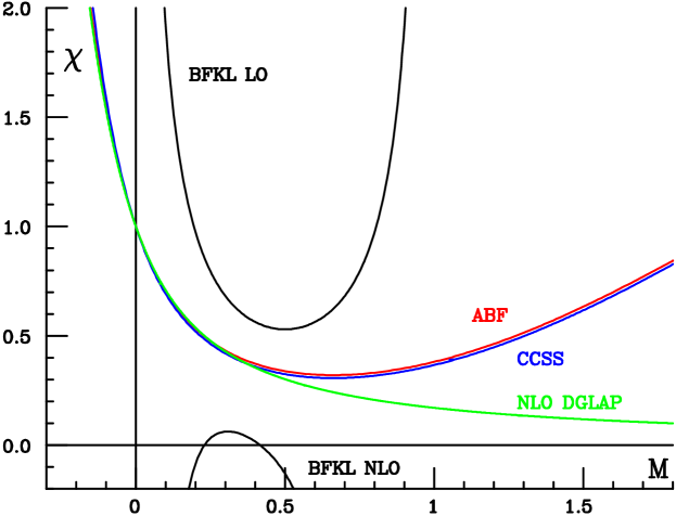
Figure 89: The kernel $\chi$ (BFKL characteristic function) for fixed coupling ($\beta_{0}=0$) $\alpha_{s}=0.2$ and ${n_{\!f}}=0$. The BFKL curves are the LO and NLO truncations of eq. (5.87), the DGLAP curve is the dual eq. (5.88) of the NLO anomalous dimension eq. (5.86), while the CCSS and ABF curves are respectively the solution $\omega$ of eq. (5.84) and the solution $\chi_{\rm DIS}$ of eq. (5.90).

The running coupling resummation procedure can be applied to a symmetrized kernel, which possesses a minimum to all orders, and then extended to next-to-leading order [217, 218]. This entails various technical complications, specifically related to the nonlinear dependence of the symmetrized kernel on $\alpha_{s}$, to the need to include interference between running coupling effects and the small $x$ resummation, and to the consistent treatment of next-to-leading log $Q^{2}$ terms, in particular those related to the running of the coupling. It should be noted that even though the ABF appraoch is limited to the description of leading-twist evolution at zero-momentum transfer, it leads to a pair of systematic dual perturbative expansions for the $\chi$ and $\gamma$ kernels. Hence, comparison with the CCSS approach is possible for instance by comparing the NLO ABF kernel to the RG improved L$x$+NL$x$ CCSS kernel.

5.3.3 Comparison of results

Even though the basic underlying physical principles of the CCSS and ABF approaches are close, there are technical differences in the construction of the resummed RG-improved (CCSS) or symmetrized DL (ABF) kernel, in the derivation from it of an anomalous dimension and associated splitting function, and in the inclusion of running coupling effects. Therefore, we will compare results for the resummed fixed-coupling $\chi$ kernel (BFKL characteristic function), then the corresponding fixed-coupling splitting functions, and finally the running coupling splitting functions which provide the final result in both approaches. In order to assess the phenomenological impact on parton evolution we will finally compare the convolution of the splitting function with a “typical” gluon distribution.

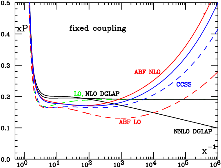
Figure 90: The fixed coupling ($\beta_{0}=0$) $xP_{gg}(x)$ splitting function, evaluated with $\alpha_{s}=0.2$ and $n_{f}=0$. The dashed curves are LO for DGLAP, NL$x$+LO for CCSS and symmetrized LO DL for ABF, while the solid curves are NLO and NNLO for DGLAP, NL$x$+NLO for CCSS and symmetrized NLO DL for ABF.

In fig. 89 we compare the solution, $\omega$, to the on-shell constraint, eq. (5.84) for the RGI CCSS result, and the solution $\chi_{\rm DIS}$ of eq. (5.90) for the symmetrized NLO DL ABF result. The pure L$x$ and NL$x$ (BFKL) and next-to-leading $\ln Q^{2}$ (DGLAP) are also shown. All curves are determined with frozen coupling ($\beta_{0}=0$), and with $n_{f}=0$, in order to avoid complications related to the diagonalization of the DGLAP anomalous dimension matrix and to the choice of scheme for the quark parton distribution. The resummed CCSS and ABF results are very close, in that they coincide by construction at the momentum conservation points $M=\frac{1}{2}$ and $M=2$, and differ only in the treatment of NLO DGLAP terms. In comparison to DGLAP, the resummed kernels have a minimum, related to the fact that both collinear and anticollinear logs are resummed. In comparison to BFKL, which has a minimum at LO but not NLO, the resummed kernels always have a perturbatively stable minimum, characterized by a lower intercept than leading–order BFKL: specifically, when $\alpha_{s}=0.2$, $\lambda\sim 0.3$ instead of $\lambda\sim 0.5$. This corresponds to a softer small $x$ rise of the associated splitting function.

The fixed–coupling resummed splitting functions up to NLO are shown in figure 90, along with the unresummed DGLAP splitting functions up to NNLO. In the CCSS approach the splitting function is determined by explicitly solving eq. (5.81) with the kernel corresponding to figure 89, and then applying the numerical deconvolution procedure of [240]. For ${n_{\!f}}=0$ the NLO DGLAP splitting function has the property that it vanishes at small $x$ — this makes it relatively straightforward to combine not just LO DGLAP but also NLO DGLAP with the NLLx resummation. Both the CCSS NL$x$+LO and NL$x$+NLO curves are shown in figure 90. On the other hand, in the ABF approach the splitting function is the inverse Mellin transform of the anomalous dimension obtained using duality eq. (5.88) from the symmetrized DL $\chi$ kernel. Hence, the LO and NLO resummed result respectively reproduce all information contained in the LO and NLO $\chi$ and $\gamma$ kernel with the additional constraint of collinear-anticollinear symmetry. Both the ABF LO and NLO results are shown in figure 90.

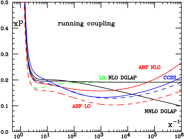
Figure 91: The running coupling $xP_{gg}(x)$ splitting function, evaluated with $\alpha_{s}=0.2$ and $n_{f}=0$. The various curves correspond to the same cases as in figure 90.

In comparison to unresummed results, the resummed splitting functions display the characteristic rise at small $x$ of fixed-coupling leading-order BFKL resummation, though the small $x$ rise is rather milder ($\sim x^{-0.3}$ instead of $\sim x^{-0.5}$ for $\alpha_{s}=0.2$). At large $x$ there is good agreement between the resummed results and the corresponding LO (dashed) or NLO (solid) DGLAP curves. At small $x$ the difference between the ABF LO and CCSS NL$x$+LO (dashed) curves is mostly due to the inclusion in CCSS of BFKL NL$x$ terms, as well as to differences in the symmetrization procedure. When comparing CCSS NL$x$+NLO with ABF NLO this difference is reduced, and , being only due the way the symmetrization is implemented, it might be taken as an estimate of the intrinsic ambiguity of the fixed–coupling resummation procedure. At intermediate $x$ the NLO resummed splitting functions is of a similar order of magnitude as the NLO DGLAP result even down to quite small $x$, but with a somewhat different shape, characterized by a shallow dip at $x\sim 10^{-2}$, until the small $x$ rise sets in for $x\sim 10^{-3}$. It has been suggested [243] that in the small ${\alpha_{\mathrm{s}}}$ limit this dip can be explained as a consequence of the interplay between the $-{\alpha_{\mathrm{s}}}^{3}\ln x$ NNLO term of $xP_{gg}$ (also present in the resummation) and the first positive resummation effects which start with an ${\alpha_{\mathrm{s}}}^{4}\ln^{3}1/x$ term. The unstable small $x$ drop of the NNLO DGLAP result appears to be a consequence of the unresummed $\frac{\alpha_{s}^{3}}{N^{2}}$ double pole in the NNLO anomalous dimension.

The running-coupling resummed splitting functions are displayed in figure 91. Note that the unresummed curves are the same as in the fixed coupling case since their dependence on $\alpha_{s}$ is just through a prefactor of $\alpha_{s}^{k}$, whereas in the resummed case there is an interplay between the running of the coupling and the structure of the small-$x$ logs. All the resummed curves display a considerable softening of the small $x$ behaviour in comparison to their fixed-coupling counterparts, due to the softening of the leading small $x$ singularity in the running-coupling case [210, 215]. As a consequence, the various resummed results are closer to each other than in the fixed-coupling case, and also closer to the unresummed LO and NLO DGLAP results. The resummed perturbative expansion appears to be stable, subject to moderate theoretical ambiguity, and qualitatively close to NLO DGLAP.

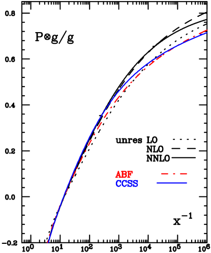
Figure 92: Convolution of resummed and fixed-order $P_{gg}$ splitting functions with a toy gluon distribution, eq. (5.92), normalised to the gluon distribution itself, with $\alpha_{s}=0.2$ and ${n_{\!f}}=0$. The resummed CCSS and ABF curves are obtained using respectively the CCSS NL$x$+NLO and the ABF NLO splitting function shown in fig. 91.

Finally, to appreciate the impact of resummation it is useful to investigate not only the properties of the splitting function, but also its convolution with a physically reasonable gluon distribution. We take the following toy gluon

$$xg(x)=x^{-0.18}(1-x)^{5}\,,$$ (5.92)

and show in fig. 92 the result of its convolution with various splitting functions of fig. 91. The differences between resummed and unresummed results, and between the CCSS and ABF resummations are partly washed out by the convolution, even though the difference between the unresummed LO and NLO DGLAP results is clearly visible. In particular, differences between the fixed-order and resummed convolution start to become significant only for $x\lesssim 10^{-2}-10^{-3}$, even though resummation effects started to be visible in the splitting functions at somewhat larger $x$.

It should be kept in mind that it is only the $gg$ entry of the singlet splitting function matrix that has so far been investigated at this level of detail and that the other entries may yet reserve surprises.

5.3.4 Explicit solution of the BFKL equation by Regge exponentiation

The CCSS approach of section 5.3.1 exploits a numerical solution of the BFKL equation in which the gluon Green’s function is represented on a grid in $x$ and $k$. This method provides an efficient determination of the azimuthally averaged Green’s function and splitting functions — for percent accuracy, up to $Y=30$, it runs in a few seconds — for a wide range of physics choices, e.g. pure NL$x$, various NL$x$+NLO schemes. Here we will discuss an alternative framework suitable to solve numerically the NLL BFKL integral equation [244], based on Monte Carlo generation of events, which can also be applied to the study of different resummation schemes and DIS, but so far has been investigated for simpler NLL BFKL kernels and Regge–like configurations. This method has the advantage that it automatically provides information about azimuthal decorrelations as well as the pattern of final-state emissions.

This appproach relies on the fact that, as shown in Ref. [244], it is possible to trade the simple and double poles in $\epsilon$, present in $D=4+2\epsilon$ dimensional regularisation, by a logarithmic dependence on an effective gluon mass $\lambda$. This $\lambda$ dependence numerically cancels out when the full NLL BFKL evolution is taken into account for a given center–of–mass energy, a consequence of the infrared finiteness of the full kernel. The introduction of this mass scale, differently to the original work of Ref. [114] was performed without angular averaging the NLL kernel.

With such reguralisation of the infrared divergencies it is then convenient to iterate the NLL BFKL equation for the $t$–channel partial wave, generating, in this way, multiple poles in the complex $\omega$–plane. The positions of these singularities are set at different values of the gluon Regge trajectory depending on the transverse momenta of the Reggeized gluons entering the emission vertices. At this point it is possible to Mellin transform back to energy space and obtain an iterated form for the solution of the NLL BFKL equation:

$$f({\bf k}_{a},{\bf k}_{b},{\rm Y}) =e^{\omega_{0}^{\lambda}\left({\bf k}_{a}\right){\rm Y}}\frac{}{}\delta^{(2)}({\bf k}_{a}-{\bf k}_{b})$$ (5.93)

$$+\sum_{n=1}^{\infty}\prod_{i=1}^{n}\int d^{2}{\bf k}_{i}\int_{0}^{y_{i-1}}dy_{i}\left[\frac{\theta\left({\bf k}_{i}^{2}-\lambda^{2}\right)}{\pi{\bf k}_{i}^{2}}\xi\left({\bf k}_{i}\right)+\widetilde{\mathcal{K}}_{r}\left({\bf k}_{a}+\sum_{l=0}^{i-1}{\bf k}_{l},{\bf k}_{a}+\sum_{l=1}^{i}{\bf k}_{l}\right)\frac{}{}\right]$$

$$\times e^{\omega_{0}^{\lambda}\left({\bf k}_{a}+\sum_{l=1}^{i-1}{\bf k}_{l}\right)(y_{i-1}-y_{i})}\ e^{\omega_{0}^{\lambda}\left({\bf k}_{a}+\sum_{l=1}^{i}{\bf k}_{l}\right)y_{n}}\delta^{(2)}\left(\sum_{l=1}^{n}{\bf k}_{l}+{\bf k}_{a}-{\bf k}_{b}\right),$$

where the strong ordering in longitudinal components of the parton emission is encoded in the nested integrals in rapidity with an upper limit set by the logarithm of the total energy in the process, $y_{0}={\rm Y}$. The first term in the expansion corresponds to two Reggeized gluons propagating in the $t$–channel with no additional emissions. The exponentials carry the dependence on the Regge gluon trajectory, i.e.

$$\omega_{0}^{\lambda}\left({\bf q}\right) = -\bar{\alpha}_{s}\ln{\frac{{\bf q}^{2}}{\lambda^{2}}}+\frac{\bar{\alpha}_{s}^{2}}{4}\left[\frac{\beta_{0}}{2N_{c}}\ln{\frac{{\bf q}^{2}}{\lambda^{2}}}\ln{\frac{{\bf q}^{2}\lambda^{2}}{\mu^{4}}}+\left(\frac{\pi^{2}}{3}-\frac{4}{3}-\frac{5}{3}\frac{\beta_{0}}{N_{c}}\right)\ln{\frac{{\bf q}^{2}}{\lambda^{2}}}+6\zeta(3)\right],$$ (5.94)

corresponding to no–emission probabilities between two consecutive effective vertices. Meanwhile, the real emission is built out of two parts, the first one:

$$\xi\left({\rm X}\right) \equiv \bar{\alpha}_{s}+\frac{{\bar{\alpha}_{s}}^{2}}{4}\left(\frac{4}{3}-\frac{\pi^{2}}{3}+\frac{5}{3}\frac{\beta_{0}}{N_{c}}-\frac{\beta_{0}}{N_{c}}\ln{\frac{{\rm X}}{\mu^{2}}}\right),$$ (5.95)

which cancels the singularities present in the trajectory order by order in perturbation theory, and the second one: $\tilde{\cal K}_{r}$, which, although more complicated in structure, does not generate $\epsilon$ singularities when integrated over the full phase space of the emissions, for details see Ref. [244].

The numerical implementation and analysis of the solution as in Eq. (5.93) was performed in Ref. [245]. As in previous studies the intercept at NLL was proved to be lower than at leading–logarithmic (LL) accuracy. In this approach the kernel is not expanded on a set of functions derived from the LL eigenfunctions, and there are no instabilities in energy associated with a choice of functions breaking the $\gamma\leftrightarrow 1-\gamma$ symmetry, with $\gamma$ being the variable Mellin–conjugate of the transverse momenta. This is explicitly shown at the left hand side of Fig. 93 where the coloured bands correspond to uncertainties from the choice of renormalisation scale.

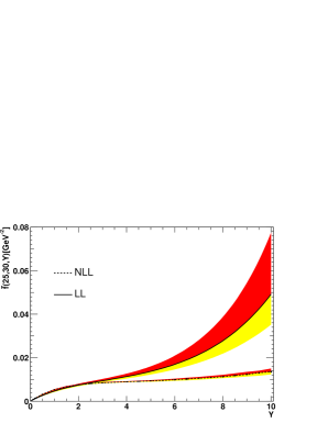
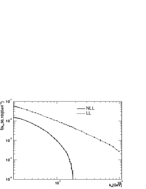
Figure 93: Analysis of the gluon Green’s function as obtained from the NLL BFKL equation. The plot to the left shows the evolution in rapidity of the gluon Green’s function at LL and NLL for fixed $k_{a}=25$ GeV and $k_{b}=30$ GeV. The plot on the right hand side shows the dependence on $k_{a}$ for fixed $k_{b}=30$ GeV and $Y=10$.

Since the exponential growth at NLL is slower than at LL, there is little overlap between the two predictions, and furthermore these move apart for increasing rapidities. The NLL corrections to the intercept amount to roughly 50% and are stable with increasing rapidities.

In transverse momentum space the NLL corrections are stable when the two transverse scales entering the forward gluon Green’s function are of similar magnitude. However, when the ratio between these scales departs largely from unity, the perturbative convergence is poor, driving, as it is well–known, the gluon Green’s function into an oscillatory behaviour with regions of negative values along the period of oscillation. This behaviour is demonstrated in the second plot of Fig 93.

The way the perturbative expansion of the BFKL kernel is improved by simultaneous resummation of energy and collinear logs has been discussed in sections 5.3.1,5.3.2. In particular, the original approach based on the introduction in the NLL BFKL kernel of an all order resummation of terms compatible with renormalisation group evolution described in ref. [238] (and incorporated in the CCSS approach of section 5.3.1) can be implemented in the iterative method here explained [246] (the method of ref. [238] was combined with the imposition of a veto in rapidities in refs. [247, 248, 249]). The main idea is that the solution to the $\omega$–shift proposed in ref. [238]

$$\omega = {\bar{\alpha}}_{s}\left(1+\left({\rm a}+\frac{\pi^{2}}{6}\right){\bar{\alpha}}_{s}\right)\left(2\psi(1)-\psi\left(\gamma+\frac{\omega}{2}-{\rm b}\,{\bar{\alpha}}_{s}\right)-\psi\left(1-\gamma+\frac{\omega}{2}-{\rm b}\,{\bar{\alpha}}_{s}\right)\right)$$ (5.96)

$$+ {\bar{\alpha}}_{s}^{2}\left(\chi_{1}\left(\gamma\right)+\left(\frac{1}{2}\chi_{0}\left(\gamma\right)-{\rm b}\right)\left(\psi^{\prime}(\gamma)+\psi^{\prime}(1-\gamma)\right)-\left({\rm a}+\frac{\pi^{2}}{6}\right)\chi_{0}(\gamma)\right),$$

can be very accurately approximated by the sum of the approximated solutions to the shift at each of the poles in $\gamma$ of the LL eigenvalue of the BFKL kernel. This provides an effective “solution” of Eq. (5.96) of the form [246]

$$\omega = \bar{\alpha}_{s}\chi_{0}(\gamma)+\bar{\alpha}_{s}^{2}\chi_{1}(\gamma)+\left\{\sum_{m=0}^{\infty}\left[\left(\sum_{n=0}^{\infty}\frac{(-1)^{n}(2n)!}{2^{n}n!(n+1)!}\frac{\left({\bar{\alpha}}_{s}+{\rm a}\,{\bar{\alpha}}_{s}^{2}\right)^{n+1}}{\left(\gamma+m-{\rm b}\,{\bar{\alpha}}_{s}\right)^{2n+1}}\right)\right.\right.$$ (5.97)

$$- \left.\left.\frac{\bar{\alpha}_{s}}{\gamma+m}-\bar{\alpha}_{s}^{2}\left(\frac{\rm a}{\gamma+m}+\frac{\rm b}{(\gamma+m)^{2}}-\frac{1}{2(\gamma+m)^{3}}\right)\right]+\left\{\gamma\rightarrow 1-\gamma\right\}\right\},$$

where $\chi_{0}$ and $\chi_{1}$ are, respectively, the LL and NLL scale invariant components of the kernel in $\gamma$ representation with the collinear limit

$$\chi_{1}\left(\gamma\right)\simeq\frac{\rm a}{\gamma}+\frac{\rm b}{\gamma^{2}}-\frac{1}{2\gamma^{3}},\,\,{\rm a}=\frac{5}{12}\frac{\beta_{0}}{N_{c}}-\frac{13}{36}\frac{n_{f}}{N_{c}^{3}}-\frac{55}{36},\,\,{\rm b}=-\frac{1}{8}\frac{\beta_{0}}{N_{c}}-\frac{n_{f}}{6N_{c}^{3}}-\frac{11}{12}.$$ (5.98)

The numerical solution to Eq. (5.96) and the value of expression (5.97) are compared in Fig. 94.

Figure 94: The $\gamma$–representation of the LL and NLL scale invariant kernels together with the collinearly–improved kernel by an $\omega$–shift and the “all–poles” resummation.

The stability of the perturbative expansion is recovered in all regions of transverse momenta with a prediction for the intercept of 0.3 at NLL for $\bar{\alpha}_{s}=0.2$, a result valid up to the introduction of scale invariance breaking terms. The implementation of expression (5.97) in transverse momentum space is simple given that the transverse components decouple from the longitudinal in this form of the collinear resummation [246]. The prescription is to remove the term $-\frac{\bar{\alpha}_{s}^{2}}{4}\ln^{2}{\frac{q^{2}}{k^{2}}}$ from the real emission kernel, ${\cal K}_{r}\left(\vec{q},\vec{k}\right)$, and replace it with

$$\left(\frac{q^{2}}{k^{2}}\right)^{-{\rm b}{\bar{\alpha}}_{s}\frac{\left|k-q\right|}{k-q}}\sqrt{\frac{2\left({\bar{\alpha}}_{s}+{\rm a}\,{\bar{\alpha}}_{s}^{2}\right)}{\ln^{2}{\frac{q^{2}}{k^{2}}}}}J_{1}\left(\sqrt{2\left({\bar{\alpha}}_{s}+{\rm a}\,{\bar{\alpha}}_{s}^{2}\right)\ln^{2}{\frac{q^{2}}{k^{2}}}}\right)-{\bar{\alpha}}_{s}-{\rm a}\,{\bar{\alpha}}_{s}^{2}+{\rm b}\,{\bar{\alpha}}_{s}^{2}\frac{\left|k-q\right|}{k-q}\ln{\frac{q^{2}}{k^{2}}},$$ (5.99)

with $J_{1}$ the Bessel function of the first kind. This prescription does not affect angular dependences and generates a well–behaved gluon Green’s function as can be seen in Fig. 95 where the oscillations in the collinear and anticollinear regions of phase space are consistently removed.

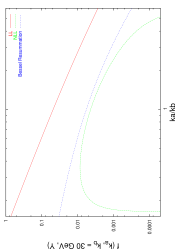
Figure 95: The behaviour of the NLL gluon Green’s function using the Bessel resummation.

At present, work is in progress to study the effect of the running of the coupling in this analysis when the Bessel resummation is introduced in the iterative procedure of Ref. [244].

A great advantage of the iterative method here described is that the solution to the NLL BFKL equation is generated integrating the phase space using a Monte Carlo sampling of the different parton configurations. This allows for an investigation of the diffusion properties of the BFKL kernel as shown in ref. [250], and provides a good handle on the average multiplicities and angular dependences of the evolution. Multiplicities can be extracted from the Poisson–like distribution in the number of iterations of the kernel needed to reach a convergent solution, which is obtained numerically at the left hand side of Fig. 96 for a fixed value of the $\lambda$ parameter. On the right hand side of the figure a study of the azimuthal angular correlation of the gluon Green’s function is presented at $Y=5$. This decorrelation will directly impact the prediction for the azimuthal angular decorrelation of two jets with a large rapidity separation, in a fully inclusive jet sample (i.e. no rapidity gaps). The increase of the angular correlation when the NLL terms are included is a characteristic feature of these corrections. This study is possible using this approach because the NLL kernel is treated in full, without angular averaging, so there is no need to use a Fourier expansion in angular variables.

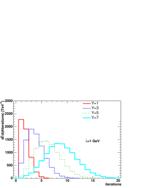
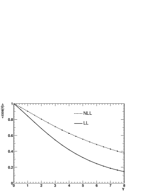
Figure 96: Distribution in the number of iterations and angular dependence of the NLL gluon Green’s function.

References

- [1] Gross, D. J. and Wilczek, F., Phys. Rev. Lett. 30, 1343 (1973)
- [2] Politzer, H. D., Phys. Rev. Lett. 30, 1346 (1973)
- [3] Gross, D. J. and Wilczek, F., Phys. Rev. D8, 3633 (1973)
- [4] Georgi, H. and Politzer, H. D., Phys. Rev. D9, 416 (1974)
- [5] Gross, D. J. and Wilczek, F., Phys. Rev. D9, 980 (1974)
- [6] Dittmar, M. and Pauss, F. and Zurcher, D., Phys. Rev. D56, 7284 (1997)
- [7] Acosta, D. et al., Phys. Rev. Lett. 94, 091803 (2005)
- [8] Bellavance, A. M., W / z production cross sections and asymmetries at e(cm) = 2-tev. Preprint hep-ex/0506025, 2005
- [9] Abazov, V. M. et al., Phys. Rev. Lett. 95, 051802 (2005)
- [10] Taffard, A., Top production cross section from cdf. To appear in the proceedings of 32nd International Conference on High-Energy Physics (ICHEP 04), Beijing, China, 16-22 Aug 2004
- [11] Bortoletto, D., Searching for susy at the tevatron. Preprint hep-ex/0412013, 2004
- [12] Heister, A. et al., Eur. Phys. J. C38, 147 (2004)
- [13] Abbiendi, G. et al., Phys. Lett. B609, 212 (2005)
- [14] Heister, A. et al., Eur. Phys. J. C28, 1 (2003)
- [15] Abdallah, J. et al., Eur. Phys. J. C37, 405 (2004)
- [16] Chekanov, S. et al., Phys. Rev. D67, 012007 (2003)
- [17] Giele, W. and Whalley, M. R., Lhapdf v3: Les houches accord pdf. Available on http://durpdg.dur.ac.uk/lhapdf/
- [18] Pumplin, J. et al., JHEP 07, 012 (2002)
- [19] Martin, A. D. et al., Eur. Phys. J C23, 73 (2002)
- [20] Corcella, G. et al., JHEP 01, 010 (2001)
- [21] Frixione, S. and Webber, B. R., JHEP 06, 029 (2002)
- [22] Stirling, W. J., private communication
- [23] Barlow, R., ECONF C030908, WEMT002 (2003)
- [24] Altarelli, G. and Parisi, G., Nucl.Phys. B126, 298 (1977)
- [25] Gribov, V.N. and Lipatov, L.N., Sov.J.Nucl.Phys 15, 438 (1972)
- [26] Lipatov, L. N., Sov.J.Nucl.Phys 20, 94 (1975)
- [27] Dokshitzer, Yu. L., JETP 46, 641 (1977)
- [28] Lipatov, L. N., Sov. J. Nucl. Phys. 23, 338 (1976)
- [29] Kuraev, E. A. and Lipatov, L. N. and Fadin, Victor S., Sov. Phys. JETP 45, 199 (1977)
- [30] Balitsky, I. I. and Lipatov, L. N., Sov. J. Nucl. Phys. 28, 822 (1978)
- [31] Devenish, R. C. E. and Cooper-Sarkar, A. M., Deep Inelastic Scattering. Oxford Unviersity Press, Oxford, 2004
- [32] Campbell, J. M. and Ellis, R. K., Mcfm v4.0: A monte carlo for femtobarn processes at hadron colliders. Available on http://mcfm.fnal.gov//
- [33] Stump, D. et al., JHEP 10, 046 (2003)
- [34] Martin, A. D. and Roberts, R. G. and Stirling, W. J. and Thorne, R. S., Eur. Phys. J. C28, 455 (2003)
- [35] Jones, R. W. L. and Ford, M. and Salam, G. P. and Stenzel, Hasko and Wicke, Daniel, JHEP 12, 007 (2003)
- [36] Anastasiou, C. and Dixon, L. J. and Melnikov, K. and Petriello, F., Phys. Rev. D69, 094008 (2004)
- [37] Dixon, L., private communication
- [38] Brun, R. and Rademakers, F., Nucl. Instrum. Meth. A389, 81 (1997)
- [39] Martin, A. D. and Roberts, R. G. and Stirling, W. J. and Thorne, R. S., Phys. Lett. B531, 216 (2002)
- [40] Alekhin, S., Phys. Rev. D68, 014002 (2003)
- [41] Adloff, C. et al., Eur. Phys. J. C21, 33 (2001)
- [42] Bassler, U. Thesis, Université Pierre et Marie Curie, Paris, 2003
- [43] Laštovička, T., Eur. Phys. J. C24, 529 (2002)
- [44] Laštovička, T., Acta Phys. Polon. B33, 2867 (2002)
- [45] ZEUS Coll., Chekanov, S. et al., Phys. Rev. D67, 012007 (2003)
- [46] ZEUS Coll., Chekanov, S. et al., Eur.Phys.J C42, 1 (2005)
- [47] Adloff, C. et al., Eur. Phys. J. C30, 1 (2003)
- [48] Eidelman, S. et al., Phys. Lett. B592, 1 (2004)
- [49] Cooper-Sarkar, A. M., J. Phys. G28, 2669 (2002)
- [50] Thorne, R.S. and Roberts, R.G., Phys. Rev D57, 6871 (1998)
- [51] Pascaud, C. and Zomer, F., Qcd analysis from the proton structure function f2 measurement: Issues on fitting, statistical and systematic errors. LAL-95-05
- [52] Adloff, C. et al., Eur. Phys. J. C13, 609 (2000)
- [53] Adloff, C. et al., Eur. Phys. J. C19, 269 (2001)
- [54] Chekanov, S. et al., Eur. Phys. J. C21, 443 (2001)
- [55] Breitweg, J. et al., Eur. Phys. J. C12, 411 (2000)
- [56] Chekanov, S. et al., Eur. Phys. J. C28, 175 (2003)
- [57] ZEUS Coll., Chekanov, S. et al., Phys. Lett. B539, 197 (2002)
- [58] Chekanov, S. and others, Phys. Rev. D70, 052001 (2004)
- [59] ZEUS Coll., Chekanov, S. et al., Eur. Phys. J. C32, 16 (2003)
- [60] Callan, Curtis G. , Jr. and Gross, David J., Phys. Rev. Lett. 22, 156 (1969)
- [61] Altarelli, Guido and Martinelli, G., Phys. Lett. B76, 89 (1978)
- [62] Cooper-Sarkar, Amanda M. and Ingelman, G. and Long, K. R. and Roberts, R. G. and Saxon, D. H., Z. Phys. C39, 281 (1988)
- [63] Moch, S. and Vermaseren, J. A. M. and Vogt, A., Phys. Lett. B606, 123 (2005)
- [64] Bartels, Jochen and Golec-Biernat, K. and Peters, K., Eur. Phys. J. C17, 121 (2000)
- [65] Adloff, C. and others, Phys. Lett. B393, 452 (1997)
- [66] Adloff, C. and others, Determination of the longitudinal proton structure function f(l)(x,q**2) at low q**2. Preprint CH1prelim-03-043. To appear in the proceedings of 32nd International Conference on High-Energy Physics (ICHEP 04), Beijing, China, 16-22 Aug 2004
- [67] Adloff, C. and others, Phys. Lett. B520, 183 (2001)
- [68] Klein, M., On the future measurement of the longitudinal structure function at low x at hera. Prepared for 12th International Workshop on Deep Inelastic Scattering (DIS 2004), Strbske Pleso, Slovakia, 14-18 Apr 2004
- [69] Feltesse, J., On a measurement of the longitudinal structure function at hera. Preprint in preparation. Talk at the Ringberg Workshop (October 2005), to be published in the proceedings
- [70] Willeke, J, Prospects for operating hera with lower proton energy at hera. Preprint unpublished memo (October 2005)
- [71] Chekanov, S. et al., Phys. Lett. B553, 141 (2003)
- [72] Towell, R. S. et al., Phys. Rev. D64, 052002 (2001)
- [73] Portheault, B. Thesis, Univ. Paris XI Orsay, March 2005
- [74] Alexopoulos, T. and others, Electron deuteron scattering with hera, a letter of intent for an experimental programme with the h1 detector. DESY-03-194
- [75] Abramovicz, H. et al., A new experiment for hera. 2003. MPP-2003-62
- [76] Willeke, F. and Hoffstaetter, G. Talks at the Workshop on the Future of DIS, Durham 2001
- [77] Acosta, D. et al., Phys. Rev. D71, 051104 (2005)
- [78] Heinemann, B. Talk at this workshop
- [79] Stirling, J. Talk at the Binn workshop on LHC Physics, 2003
- [80] Strikman, M., private communication
- [81] Forte, S., private communication
- [82] Botje, M. and Klein, M. and Pascaud, C. Preprint hep-ph/9609489. HERA Physics Workshop 1996/97
- [83] Chekanov, S. et al., Phys. Lett. B547, 164 (2002)
- [84] Chekanov S. et al., Eur. Phys. J. C23, 615 (2002)
- [85] Targett-Adams, C., private communication
- [86] Frixione, S. and Ridolfi, G., Nucl. Phys., B507, 315 (1997)
- [87] Aurenche, P. and Guillet, J. and Fontannaz, M., Z. Phys. C64, 621 (1994)
- [88] Giele, W. T. and Glover, E. W. N. and Kosower, D. A., Nucl. Phys. B403, 633 (1993)
- [89] Whalley, M. R. and Bourilkov, D. and Group, R. C., The les houches accord pdfs (lhapdf) and lhaglue. Preprint hep-ph/0508110, 2005
- [90] Glück, M. and Reya, E. and Vogt, A., Z. Phys. C67, 433 (1995)
- [91] Thorne, R., private communication
- [92] Martin, A. D. and Stirling, W. J. and Roberts, R. G., Phys. Lett. B354, 155 (1995)
- [93] Martin, A. D. and Roberts, R. G. and Stirling, W. J. and Thorne, R. S., Eur. Phys. J. C35, 2004 (2004)
- [94] Graudenz, D. and Hampel, M. and Vogt, A. and Berger, C., Z. Phys. C70, 77 (1996)
- [95] Kosower, D. A., Nucl. Phys. B520, 263 (1998)
- [96] Stratmann, M. and Vogelsang, W., Phys. Rev. D64, 114007 (2001)
- [97] Wobisch, M. Thesis, RWTH Aachen, PITHA 00/12 and DESY-THESIS-2000-049, December 2000
- [98] Ratcliffe, P. G., Phys. Rev. D63, 116004 (2001)
- [99] Dasgupta, M. and Salam, G. P., Eur. Phys. J. C24, 213 (2002)
- [100] Nagy, Z., Phys. Rev. D68, 094002 (2003)
- [101] Nagy, Z., Phys. Rev. Lett. 88, 122003 (2002)
- [102] Nagy, Z. and Trocsanyi, Z., Phys. Rev. Lett. 87, 082001 (2001)
- [103] Van Neerven, W. L. and Zijlstra, E. B., Phys. Lett. B272, 127 (1991)
- [104] Zijlstra, E. B. and van Neerven, W. L., Phys. Lett. B273, 476 (1991)
- [105] Zijlstra, E. B. and van Neerven, W. L., Phys. Lett. B297, 377 (1992)
- [106] Zijlstra, E. B. and van Neerven, W. L., Nucl. Phys. B383, 525 (1992)
- [107] Moch, S. and Vermaseren, J. A. M., Nucl. Phys. B573, 853 (2000)
- [108] Moch, S. and Vermaseren, J. A. M. and Vogt, A., Nucl. Phys. B688, 101 (2004)
- [109] Vogt, A. and Moch, S. and Vermaseren, J. A. M., Nucl. Phys. B691, 129 (2004)
- [110] Vermaseren, J. A. M. and Vogt, A. and Moch, S., Nucl. Phys. B724, 3 (2005)
- [111] Moch, S. and Vermaseren, J. A. M. and Vogt, A., Nucl. Phys. B646, 181 (2002)
- [112] Moch, S. and Vermaseren, J. A. M. and Vogt, A., Nucl. Phys. Proc. Suppl. 135, 137 (2004)
- [113] Catani, S. and Hautmann, F., Nucl. Phys. B427, 475 (1994)
- [114] Fadin, V. S. and Lipatov, L. N., Phys. Lett. B429, 127 (1998)
- [115] Jaroszewicz, T., Phys. Lett. B116, 291 (1982)
- [116] Kirschner, R. and Lipatov, L. N., Nucl. Phys. B213, 122 (1983)
- [117] Blümlein, J. and Vogt, A., Phys. Lett. B370, 149 (1996)
- [118] Van Neerven, W. L. and Vogt, A., Nucl. Phys. B603, 42 (2001)
- [119] Larin, S. A. and van Ritbergen, T. and Vermaseren, J. A. M., Nucl. Phys. B427, 41 (1994)
- [120] Larin, S. A. and Nogueira, P. and van Ritbergen, T. and Vermaseren, J. A. M., Nucl. Phys. B492, 338 (1997)
- [121] Retey, A. and Vermaseren, J. A. M., Nucl. Phys. B604, 281 (2001)
- [122] Blümlein, J. and Kurth, S., Phys. Rev. D60, 014018 (1999)
- [123] Blümlein, J., Comput. Phys. Commun. 159, 19 (2004)
- [124] Remiddi, E. and Vermaseren, J. A. M., Int. J. Mod. Phys. A15, 725 (2000)
- [125] Borwein, J. M. and Bradley, D. M. and Broadhurst, D. J. and Lisonek, P., Trans. Am. Math. Soc. 353, 907 (2001)
- [126] Blümlein, J., in preparation
- [127] Blümlein, J. and Moch, S., in preparation
- [128] Blümlein, J., Nucl. Phys. Proc. Suppl. 135, 225 (2004)
- [129] Blümlein, J., Comput. Phys. Commun. 133, 76 (2000)
- [130] Blümlein, J. and Moch, S., Phys. Lett. B614, 53 (2005)
- [131] Nielsen, N., Nova Acta Leopoldina (Halle) 90, 123 (1909)
- [132] Matsuura, T. and van der Marck, S. C. and van Neerven, W. L., Nucl. Phys. B319, 570 (1989)
- [133] Hamberg, R. and van Neerven, W. L. and Matsuura, T., Nucl. Phys. B359, 343 (1991)
- [134] Ravindran, V. and Smith, J. and van Neerven, W. L., Nucl. Phys. B682, 421 (2004)
- [135] Catani, S. and de Florian, D. and Grazzini, M., JHEP 05, 025 (2001)
- [136] Harlander, R. V. and Kilgore, W. B., Phys. Rev. D64, 013015 (2001)
- [137] Harlander, R. V. and Kilgore, W. B., Phys. Rev. Lett. 88, 201801 (2002)
- [138] Harlander, R. V. and Kilgore, W. B., JHEP 10, 017 (2002)
- [139] Anastasiou, C. and Melnikov, K., Nucl. Phys. B646, 220 (2002)
- [140] Ravindran, V. and Smith, J. and van Neerven, W. L., Nucl. Phys. B665, 325 (2003)
- [141] Rijken, P. J. and van Neerven, W. L., Phys. Lett. B386, 422 (1996)
- [142] Rijken, P. J. and van Neerven, W. L., Nucl. Phys. B487, 233 (1997)
- [143] Rijken, P. J. and van Neerven, W. L., Phys. Lett. B392, 207 (1997)
- [144] Blümlein, J. and Ravindran, V., Nucl. Phys. Proc. Suppl. 135, 24 (2004)
- [145] Blümlein, J. and Ravindran, V., Nucl. Phys. B716, 128 (2005)
- [146] Blümlein, J. and Böttcher, H. and Guffanti, A., Nucl. Phys. Proc. Suppl. 135, 152 (2004)
- [147] Blumlein, J. and Bottcher, H. and Guffanti, A., in preparation
- [148] Alekhin, S., Phys. Rev. D63, 094022 (2001)
- [149] Botje, M. and Klein, M. and Pascaud, C. (1996)
- [150] Blümlein, J. and Riemersma, S. and van Neerven, W. L. and Vogt, A., Nucl. Phys. Proc. Suppl. 51C, 97 (1996)
- [151] Blümlein, J. and Guffanti, A., Scheme-invariant nnlo evolution for unpolarized dis structure functions. Preprint hep-ph/0411110, 2004
- [152] Furmanski, W. and Petronzio, R., Zeit. Phys. C11, 293 (1982)
- [153] Catani, S., Z. Phys. C75, 665 (1997)
- [154] Blümlein, J. and Ravindran, V. and van Neerven, W. L., Nucl. Phys. B586, 349 (2000)
- [155] Alekhin, S. and Blümlein, J., Phys. Lett. B594, 299 (2004)
- [156] Giele, W. et al, The qcd/sm working group: Summary report. Preprint hep-ph/0204316, 2002
- [157] Blümlein, J. and Böttcher, H., Nucl. Phys. B636, 225 (2002)
- [158] Van Neerven, W. L. and Vogt, A., Phys. Lett. B490, 111 (2000)
- [159] Blümlein, J. et al., A detailed comparison of nlo qcd evolution codes. Preprint hep-ph/9609400, 1996
- [160] Vogt, A., Comput. Phys. Commun. 170, 65 (2005)
- [161] Lai, H. L. et al., Eur. Phys. J. C12, 375 (2000)
- [162] Buza, M. and Matiounine, Y. and Smith, J. and van Neerven, W. L., Eur. Phys. J. C1, 301 (1998)
- [163] Chuvakin, A. and Smith, J., Comput. Phys. Commun. 143, 257 (2002)
- [164] Larin, S. A. and van Ritbergen, T. and Vermaseren, J. A. M., Nucl. Phys. B438, 278 (1995)
- [165] Chetyrkin, K. G. and Kniehl, B. A. and Steinhauser, M., Phys. Rev. Lett. 79, 2184 (1997)
- [166] Alwall, J. and Ingelman, G., Phys. Rev. D71, 094015 (2005)
- [167] Alwall, J. and Ingelman, G., Phys. Rev. D70, 111505 (2004)
- [168] Alwall, J. and Ingelman, G., Phys. Lett. B596, 77 (2004)
- [169] Whitlow, L. W. and Riordan, E. M. and Dasu, S. and Rock, Stephen and Bodek, A., Phys. Lett. B282, 475 (1992)
- [170] Benvenuti, A. C. et al., Phys. Lett. B223, 485 (1989)
- [171] Benvenuti, A. C. et al., Phys. Lett. B237, 592 (1990)
- [172] Arneodo, M. et al., Nucl. Phys. B483, 3 (1997)
- [173] Kazakov, D. I. and Kotikov, A. V., Phys. Lett. B291, 171 (1992)
- [174] Alekhin, S., Parton distribution functions from the precise nnlo qcd fit. Preprint hep-ph/0508248, 2005
- [175] Huston, J. and Pumplin, J. and Stump, D. and Tung, W. K., JHEP 06, 080 (2005)
- [176] Altarelli, G. and Ball, R. D. and Forte, S., Nucl. Phys. B674, 459 (2003)
- [177] Moreno, G. et al., Phys. Rev. D43, 2815 (1991)
- [178] Anastasiou, C. and Dixon, L. J. and Melnikov, K. and Petriello, F., Phys. Rev. Lett. 91, 182002 (2003)
- [179] Bazarko, A. O. et al., Z. Phys. C65, 189 (1995)
- [180] Alekhin, S., Statistical properties of the estimator using covariance matrix. Preprint hep-ex/0005042, 2000
- [181] Botje, M., Eur. Phys. J. C14, 285 (2000)
- [182] Giele, W.T. and Keller, S., Phys. Rev. D58, 094023 (1998)
- [183] Giele, Walter T. and Keller, Stephane A. and Kosower, David A., Parton distribution function uncertainties. Preprint hep-ph/0104052, 2001
- [184] Whalley, M., talk at this workshop
- [185] Webb, J. C. and others, Absolute drell-yan dimuon cross sections in 800-gev/c p p and p d collisions. Preprint hep-ex/0302019, 2003
- [186] Abbott, T. et al., Phys. Rev. Lett. 86, 1707 (2001)
- [187] Affolder, T. et al., Phys. Rev. D64, 032001 (2001)
- [188] Pumplin, J. and Stump, D. R. and Tung, W. K., Phys. Rev. D65, 014011 (2002)
- [189] Stump, D. et al., Phys. Rev. D65, 014012 (2002)
- [190] Pumplin, J. et al., Phys. Rev. D65, 014013 (2002)
- [191] Martin, A. D. and Roberts, R. G. and Stirling, W. J. and Thorne, R. S., Phys. Lett. B604, 61 (2004)
- [192] Alekhin, S., Nnlo parton distributions from deep-inelastic scattering data. Preprint hep-ph/0311184, 2003
- [193] Pumplin, J. et al., Parton distributions. Preprint hep-ph/0507093, 2005
- [194] Stump, D. et al., JHEP 10, 046 (2003)
- [195] Forte, S. and Garrido, L. and Latorre, J. I. and Piccione, A., JHEP 05, 062 (2002)
- [196] Del Debbio, L. and Forte, S. and Latorre, J. I. and Piccione, A. and Rojo, J., JHEP 03, 080 (2005)
- [197] Rojo, J. and Latorre, J. I., JHEP 01, 055 (2004)
- [198] Rojo, J. and Del Debbio, L. and Forte, S. and Latorre, J. I. and Piccione, A., The neural network approach to parton fitting. Preprint hep-ph/0505044, 2005
- [199] Sterman, G., Nucl. Phys. B281, 310 (1987)
- [200] Catani, S. and Trentadue, L., Nucl. Phys. B327, 323 (1989)
- [201] Forte, S. and Ridolfi, G., Nucl. Phys. B650, 229 (2003)
- [202] Vogt, A., Phys. Lett. B497, 228 (2001)
- [203] Moch, S. and Vermaseren, J. A. M. and Vogt, A., Nucl. Phys. B726, 317 (2005)
- [204] Moch, S. and Vogt, A., Higher-order soft corrections to lepton pair and higgs boson production. Preprint hep-ph/0508265, 2005
- [205] Laenen, E. and Magnea, L., Threshold resummation for electroweak annihilation from dis data. Preprint hep-ph/0508284, 2005
- [206] Eynck, T. O. and Laenen, E. and Magnea, L., JHEP 06, 057 (2003)
- [207] Lipatov, L. N., Sov. Phys. JETP 63, 904 (1986)
- [208] Camici, G. and Ciafaloni, M., Phys. Lett. B412, 396 (1997)
- [209] Ciafaloni, M. and Camici, G., Phys. Lett. B430, 349 (1998)
- [210] Ciafaloni, M. and Colferai, D. and Salam, G. P., Phys. Rev. D60, 114036 (1999)
- [211] Ciafaloni, M. and Colferai, D. and Colferai, D. and Salam, G. P. and Stasto, A. M., Phys. Lett. B576, 143 (2003)
- [212] Ciafaloni, M. and Colferai, D. and Salam, G. P. and Stasto, A. M., Phys. Rev. D68, 114003 (2003)
- [213] Altarelli, G. and Ball, R. D. and Forte, S., Nucl. Phys. B575, 313 (2000)
- [214] Altarelli, G. and Ball, R. D. and Forte, S., Nucl. Phys. B599, 383 (2001)
- [215] Altarelli, G. and Ball, R. D. and Forte, S., Nucl. Phys. B621, 359 (2002)
- [216] Altarelli, G. and Ball, R. D. and Forte, S., An improved splitting function for small x evolution. Preprint hep-ph/0310016, 2003
- [217] Altarelli, G. and Ball, R. D. and Forte, S., Nucl. Phys. Proc. Suppl. 135, 163 (2004)
- [218] Altarelli, G. and Ball, R. D. and Forte, S., Perturbatively stable resummed small kernels. Preprint CERN-PH-TH/2005-174, 2005
- [219] Catani, S. and Mangano, Michelangelo L. and Nason, Paolo and Oleari, Carlo and Vogelsang, Werner, JHEP 03, 025 (1999)
- [220] Laenen, E. and Sterman, G. and Vogelsang, W., Phys. Rev. Lett. 84, 4296 (2000)
- [221] Kidonakis, N. and Sterman, G., Nucl. Phys. B505, 321 (1997)
- [222] Kidonakis, N. and Owens, J. F., Phys. Rev. D63, 054019 (2001)
- [223] Laenen, E. and Moch, S., Phys. Rev. D59, 034027 (1999)
- [224] Corcella, G. and Mitov, A. D., Nucl. Phys. B676, 346 (2004)
- [225] Tzanov, M. et al., New qcd results from nutev. Preprint hep-ex/0306035, 2003
- [226] Naples, D. et al., Nutev cross section and structure function measurements. Preprint hep-ex/0307005, 2003
- [227] Corcella, G. and Magnea, L., Soft-gluon resummation effects on parton distributions. Preprint hep-ph/0506278, 2005
- [228] Ciafaloni, M. and Colferai, D., Dimensional regularisation and factorisation schemes in the bfkl equation at subleading level. Preprint hep-ph/0507106, 2005
- [229] Ball, R. D. and Forte, S., Phys. Lett. B465, 271 (1999)
- [230] Catani, S. and Ciafaloni, M. and Hautmann, F., Phys. Lett. B242, 97 (1990)
- [231] Catani, S. and Ciafaloni, M. and Hautmann, F., Nucl. Phys. B366, 135 (1991)
- [232] Collins, J. C. and Ellis, R. K., Nucl. Phys. B360, 3 (1991)
- [233] Bartels, J. and Gieseke, S. and Qiao, C. F., Phys. Rev. D63, 056014 (2001)
- [234] Bartels, J. and Gieseke, S. and Kyrieleis, A., Phys. Rev. D65, 014006 (2002)
- [235] Bartels, J. and Colferai, D. and Gieseke, S. and Kyrieleis, A., Phys. Rev. D66, 094017 (2002)
- [236] Bartels, J. and Colferai, D. and Vacca, G. P., Eur. Phys. J. C24, 83 (2002)
- [237] Bartels, J. and Colferai, D. and Vacca, G. P., Eur. Phys. J. C29, 235 (2003)
- [238] Salam, G. P., JHEP 07, 019 (1998)
- [239] Ciafaloni, M. and Colferai, D., Phys. Lett. B452, 372 (1999)
- [240] Ciafaloni, M. and Colferai, D. and Salam, G. P., JHEP 07, 054 (2000)
- [241] Ball, R. D. and Forte, S., Phys. Lett. B405, 317 (1997)
- [242] Ball, R. D. and Forte, S., Phys. Lett. B359, 362 (1995)
- [243] Ciafaloni, M. and Colferai, D. and Salam, G. P. and Stasto, A. M., Phys. Lett. B587, 87 (2004)
- [244] Andersen, J. R. and Sabio Vera, A., Phys. Lett. B567, 116 (2003)
- [245] Andersen, J. R. and Sabio Vera, A., Nucl. Phys. B679, 345 (2004)
- [246] Sabio Vera, A., Nucl. Phys. B722, 65 (2005)
- [247] Schmidt, C. R., Phys. Rev. D60, 074003 (1999)
- [248] Forshaw, J. R. and Ross, D. A. and Sabio Vera, A., Phys. Lett. B455, 273 (1999)
- [249] Chachamis, G. and Lublinsky, M. and Sabio Vera, A., Nucl. Phys. A748, 649 (2005)
- [250] Andersen, J. R. and Sabio Vera, A., JHEP 01, 045 (2005).