ICRR-Report-522-2005-5

KEK-TH-1047

Heavy Wino-like Neutralino Dark Matter Annihilation
into Antiparticles

Junji Hisano¹, Shigeki Matsumoto², Osamu Saito¹, and Masato Senami^1
1ICRR, University of Tokyo, Kashiwa 277-8582, Japan
²Theory Group, KEK, Oho 1-1 Tsukuba, Ibaraki 305-0801, Japan

1 Introduction

The existence of the cold dark matter (CDM) has been confirmed by the WMAP measurement of the cosmic microwave background [1]; $\Omega_{{\rm CDM}}h^{2}=0.113^{+0.016}_{-0.018}$ [2]. However, the nature of the dark matter (DM) still remains a mystery. Weakly Interacting Massive Particles (WIMPs) are viable candidates for the DM since their thermal relic abundances are naturally within the observed range [3].

A well-studied representative of WIMPs is the lightest neutralino in supersymmetric extensions of the standard model [4]. Neutralinos are composed of bino, neutral wino and neutral Higgsinos, which are superpartners of the U(1)_Y and SU(2)_L gauge bosons and the Higgs bosons, respectively. In most supersymmetric models, the lightest neutralino is the lightest supersymmetric particle (LSP) and is stable due to the R-parity conservation. The constituent of the neutralino depends on supersymmetry breaking models. For example, the neutralino is bino-like in a wide region of the parameter region of the minimal supergravity model. In the anomaly mediated supersymmetry breaking model (AMSB) [5], the neutralino is wino-like because gaugino masses are proportional to beta functions of the gauge coupling constants. The wino-like neutralino has larger coupling than the bino-like one, so that the wino-like neutralino DM has larger prospects for detection.

Various experiments have been performed or are planed in order to detect the neutralino DM directly or indirectly. The direct detections are to measure the recoil energy which the neutralino may deposit as it crosses a terrestrial detector [6]. The detection rate depends on the cross section for the elastic-scattering of the neutralino with target nuclei. On the other hand, the indirect ones are to detect the anomalous cosmic rays produced in the neutralino annihilation. Detectors are designed to observe high-energy neutrinos from the earth or the sun, gamma-rays from the galactic center, and antimatter cosmic rays from the galactic halo, which are generated from the neutralino annihilation.

In this paper, we consider indirect detection of the wino-like neutralino DM by positrons and antiprotons in cosmic rays. It is pointed out in Refs. [7, 8] that the cross sections for the wino-like neutralino annihilation into gauge bosons are enhanced compared with those at the tree-level approximation when the mass is larger than about 1 TeV. This is due to a non-perturbative effect by the electroweak interaction, which appears in a non-relativistic limit of the wino-like neutralinos. Especially, when the mass is around 2 TeV, which is favored from the thermal relic abundance of the wino-like neutralino [9], the annihilation cross sections are significantly enhanced by the resonance effect.

The enhancement of the annihilation cross sections raises the possibilities of the indirect detection of the wino-like neutralino DM. In Ref. [8], the gamma-ray flux produced by the wino-like neutralino annihilation in the galactic center is evaluated, and it is found that the the sensitivity for the wino-like neutralino DM is enhanced. In this paper, we evaluate the positron and antiproton fluxes from the wino-like neutralino annihilation in the galactic halo, including the non-perturbative effect. We find that, for the neutralino with mass around 2 TeV, the positron and antiproton signals also exceed the backgrounds. These fluxes will be measured with unprecedented accuracies by the upcoming experiments such as PAMELA [10] and AMS-02 [11]. Especially, the measurement of the positron flux may be more promising for detection of the wino-like neutralino with mass around 2 TeV, since the predicted positron flux is less sensitive to the astrophysical parameters responsible to the propagation or the DM halo profile.

This paper is organized as follows. In section 2, we review the non-perturbative effect on the wino-like neutralino annihilation cross sections. In section 3, the positron flux from the annihilation in the galactic halo is evaluated using the diffusion model. Here, we compare the predicted signal positron flux with the expected background, and discuss the sensitivities of the future experiments to the heavy wino-like neutralino DM. The HEAT anomaly [12] is also discussed. In section 4, we investigate the antiproton flux from the wino-like neutralino annihilation. The expected background and the future prospect are also discussed. Section 5 is devoted to conclusions.

2 Non-perturbative effect on wino-like neutralino annihilation

The wino-like neutralinos annihilate mainly into $W$ bosons due to the SU(2)_L gauge interaction. The annihilation process is mediated by $t$-channel wino-like chargino exchange at tree-level, and the cross section is given by

$$\sigma v=\frac{2\pi\alpha_{2}^{2}}{m^{2}}~{},$$ (1)

where $v$ is the relative velocity of the neutralinos, $\alpha_{2}$ is the SU(2)_L gauge coupling constant and $m$ is the wino mass.

We take a non-relativistic limit ($v\ll 1$) in Eq. (1), however, the tree-level approximation in the limit is not valid for the wino-like neutralino heavier than $\sim m_{W}/\alpha_{2}$. Here, $m_{W}$ is the $W$ boson mass. This is due to the threshold singularity caused by the mass degeneracy between the wino-like neutralino and chargino, and the higher-order contributions should be included in the case. The dominant contribution to the scattering amplitude at $O(\alpha_{2}^{(n+1)})$ comes from ladder diagrams, in which $n$ gauge bosons are exchanged. When the mass difference between the wino-like neutralino and chargino is negligible, the $n$-th ladder diagram is suppressed by only $(\alpha_{2}m/m_{W})^{(n)}$ compared with the leading-order one [13]. Thus, when $m$ is larger than $\sim m_{W}/\alpha_{2}$, we need to resum the diagrams at all orders. In other words, we have to include the non-perturbative effect for obtaining the reliable annihilation cross section.

The resummation of the ladder diagrams has a following interpretation. Since the wino mass is much heavier than that of the $W$ boson, the wino-like neutralinos feel the long-range force induced from the $W$ boson exchange. Due to the force, the wave function of the neutralino pair is significantly modified from the plane wave before the annihilation into $W^{+}W^{-}$ bosons. As shown in Ref. [8], the bound states, which are composed of the neutralino and chargino pairs, appear due to the long-range force if the wino mass is large enough. Especially interesting, a bound state has the binding energy almost zero when the wino mass is close to $\sim$ 2, 8, $\cdots$ TeV. In those cases, the wino-like neutralino annihilation cross section in a non-relativistic limit is enhanced by several orders of magnitude compared to that of the tree-level cross section due to the resonance.

Figure 1: Cross sections, $\sigma v$, of the annihilation of the wino-like neutralinos into $W^{+}W^{-}$ (left figure) and $ZZ$ (right figure) in a non-relativistic limit. The mass difference between the wino-like neutralino and chargino is set to be 0.1 GeV. For comparison, the cross sections at the leading order in perturbation are shown as dashed lines. The bound state resonances appear around 2 TeV and 8 TeV.

In Fig. 1, the annihilation cross sections into $W^{+}W^{-}$ and $ZZ$ bosons are shown as functions of the wino mass. These figures are plotted using fitting formulae for the wino-like neutralino annihilation cross sections given in Ref. [8]. When the mass difference between the wino-like neutralino and chargino is much smaller than $~{}\alpha_{2}m_{W}$, which is a typical potential energy due to the electroweak interaction, the cross sections are less sensitive to the value of the mass difference. In this paper, the mass difference is set to be 0.1 GeV for definiteness. For heavy wino-like neutralino, this mass difference is dominated by the radiative correction, and it is $0.1-0.2$ GeV in most of the parameters region [8]. This is because the tree-level contribution to the mass difference is suppressed by $({m_{W}}/{M_{\rm SUSY}})^{4}$ unless the wino mass is accidentally finely tuned to the Higgsino mass. The mixing between the wino and Higgsino components is also suppressed by $({m_{W}}/{M_{\rm SUSY}})$. Thus, we ignore the mixing in the following.

As shown in the figure, the annihilation cross section into $ZZ$ is also enhanced for $m\mathop{}_{\textstyle\sim}^{\textstyle>}1$ TeV in addition to that into $W^{+}W^{-}$, and it becomes comparable to that into $W^{+}W^{-}$. The cross sections into $\gamma\gamma$ and $\gamma Z$ also have a behavior similar to that into $ZZ$. The annihilation channels into $ZZ$, $\gamma Z$ and $\gamma\gamma$ come from one-loop diagrams in the perturbation, and the cross sections are suppressed. However, the transition between the neutralino pair state and the chargino pair state is not suppressed due to the non-perturbative effect for $m\mathop{}_{\textstyle\sim}^{\textstyle>}1$ TeV, so that the cross sections are enhanced. When evaluating the positron and antiproton fluxes from the wino-like neutralino annihilation in the galactic halo, we need to include the contribution of the annihilation into $Z$ bosons, in addition to that into $W$ bosons.

If the relic abundance of the wino-like neutralino in the universe is explained by the thermal scenario, the mass consistent with the WMAP observation is around 2 TeV [9]. It is intriguing that this value is coincident with the mass corresponding to the resonant annihilation as shown in Fig. 1. On the other hand, the wino-like neutralino DM is also produced by non-thermal processes such as the moduli decay [14, 15]. Furthermore, the late time entropy production by, for example, the thermal inflation [16] may decrease the amount of the DM. In these cases, the mass of the wino-like neutralino consistent with the DM observations may be deviated from 2 TeV.

In this paper, while the heavy wino-like neutralino with mass around 2 TeV is noticed, we discuss the positron and antiproton signatures from the neutralino annihilation without peculiar masses specified for completeness. Thus, we assume that the wino-like neutralino is dominant constituent of the CDM in the present universe, and exists in the halo of our galaxy with appropriate mass density in the following.

3 Positron signature of wino-like neutralino dark matter

In this section, we evaluate the positron flux from the wino-like neutralino annihilation in the galactic halo. In the evaluation of the signal flux in the vicinity of the solar system, we need to consider the propagation of positrons through the galaxy, in addition to the production rate of the positrons from the annihilation in the halo. We discuss these in order, and show the sensitivities of the upcoming experiments, such as PAMELA and AMS-02, to the positron signal by comparing the expected background originated from the secondary production of the cosmic rays. The HEAT anomaly is also discussed.

3.1 Production rate of positrons from dark matter annihilation

The production rate of positrons from the neutralino DM annihilation in the galactic halo is given as

$$Q(E,\vec{r})=\frac{1}{2}n^{2}(\vec{r})\sum_{f}\langle\sigma v\rangle_{f}\left(\frac{dN_{e^{+}}}{dE}\right)_{f}~{}~{},$$ (2)

where $n$ is the number density of the neutralinos in the galactic halo, $\langle\sigma v\rangle_{f}$ is the annihilation cross section into the final state $f$. The fragmentation function $(dN_{e^{+}}/dE)_{f}$ represents the number of positrons with energy $E$, which are produced from the final state $f$. The coefficient $1/2$ comes from the pair annihilation of the identical particles.

As discussed in the previous section, the wino-like neutralinos annihilate into $W$ and $Z$ bosons. Positrons are produced through the leptonic and hadronic cascade decays of the weak gauge bosons, for example, $W^{+}\rightarrow e^{+}\nu$, $W^{+}\rightarrow\mu^{+}\nu\rightarrow e^{+}\nu\bar{\nu}\nu$ or $W^{\pm}\rightarrow{\rm hadrons}\rightarrow\pi^{+}\rightarrow\mu^{+}\rightarrow e^{+}$. These cascade decay processes for producing positrons are encoded into the fragmentation functions $(dN_{e^{+}}/dE)_{f}$ $(f=WW$ and $ZZ$). We ignore the contribution from the annihilation into $Z\gamma$, since the contribution is less than about $10\%$. We evaluate the fragmentation functions using the HERWIG Monte-Carlo code [17] and derive the fitting functions as follows,

$$\left(\frac{dN_{e^{+}}}{dx}\right)_{WW}=\exp\left[WW(\ln(x))\right]~{},\qquad\left(\frac{dN_{e^{+}}}{dx}\right)_{ZZ}=\exp\left[ZZ(\ln(x))\right]~{},$$ (3)

where $x=E/m$ and the functions, $WW(x)$ and $ZZ(x)$, are given by

$$WW(x) = -2.28838-0.605364x-0.287614x^{2}-0.762714x^{3}$$

$$-0.319561x^{4}-0.0583274x^{5}-0.00503555x^{6}-0.00016691x^{7}~{},$$

$$ZZ(x) = -2.75588-0.45725x-0.141373x^{2}-0.905392x^{3}$$ (4)

$$-0.444098x^{4}-0.0936451x^{5}-0.00942148x^{6}-0.000369777x^{7}~{}.$$

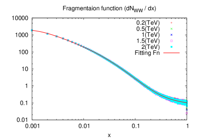
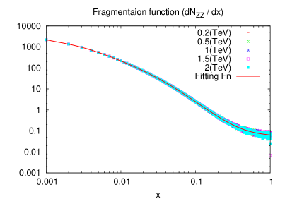
Figure 2: Fitting functions of the fragmentation functions $(dN_{e^{+}}/dx)_{WW}$ and $(dN_{e^{+}}/dx)_{ZZ}$ (solid lines) and HERWIG Monte-Carlo results in cases of $m=0.2,0.5,1,1.5$, and 2 TeV.

In Fig. 2, the fragmentation functions from the HERWIG code and the fitting functions are depicted. The results of Monte-Carlo simulations are shown for cases of $m=0.2,0.5,1,1.5$, and 2 TeV. The fitting functions are shown as solid lines and agree well with the simulation data with the range $m\gtrsim 300$ GeV and $x\gtrsim 10^{-3}$. It is found that the slopes of the fragmentation functions are changed around $x\sim 0.2$. The positrons with lower energy $(x\lesssim 0.2)$ comes from the hadronic cascade decay process [18], while those with higher energy $(x\gtrsim 0.2)$ are produced more directly from the leptonic weak boson decays.

Next, we discuss the DM number density in the galactic halo. The number density is derived from the DM halo mass profile $\rho(\vec{r})$ through the equation $n(\vec{r})=\rho(\vec{r})/m$. The halo mass profile is determined by observations of the rotational velocity of the galaxy and the motions of the dwarf galaxies with help of the $N$-bodies simulations, while several models for the DM profile are proposed. In this paper, we use the isothermal halo model, which is given as

$$\rho(\vec{r})=0.43\frac{2.8^{2}+8.5^{2}}{2.8^{2}+(r/1~{}{\rm kpc})^{2}}~{}~{}({\rm GeV/cm^{3}})~{},$$ (5)

where $r=|\vec{r}|$ is the distance from the galactic center, 0.43 GeV/cm³ is the local halo density (the mass density in the vicinity of the solar system), 2.8 kpc is the core radius of the galaxy, and 8.5 kpc is the distance between the galactic center and the solar system.

3.2 Propagation of positrons in the galaxy

Once positrons are produced by the DM annihilation, they travel in the galaxy under the influence of the tangled magnetic field. Since the typical strength of the magnetic field is a micro Gauss, the gyroradius of the positron is much less than the galactic radius. Thus, the propagation can be treated as a random walk, and only some portion of the positrons can reach to the earth.

There are some models for the propagation. Among those, we use the ‘diffusion model’ in which the random walk is described by the diffusion equation,

$$\frac{\partial}{\partial t}f_{e^{+}}(E,\vec{r})=K(E)\nabla^{2}f_{e^{+}}(E,\vec{r})+\frac{\partial}{\partial E}\left[b(E)f_{e^{+}}(E,\vec{r})\right]+Q(E,\vec{r})~{},$$ (6)

where $f_{e^{+}}(E,\vec{r})$ is the number density of positrons per unit energy, $E$ is the energy of positron, $K(E)$ is the diffusion constant, $b(E)$ is the energy loss rate, and $Q(E,\vec{r})$ is the source (positron injection) term discussed in the previous section. The flux of positrons with high energy ($E\gg m_{e}$) in the vicinity of the solar system is given from $f_{e^{+}}(E,\vec{r})$ as

$$\Phi_{e^{+}}(E)=\frac{c}{4\pi}f_{e^{+}}(E,\vec{r}_{\odot})~{},$$ (7)

where $c$ is the velocity of light and $\vec{r}_{\odot}$ represents the coordinate of the solar system.

The diffusion constant $K(E)$ in Eq. (6) is obtained by the simulation of cosmic rays, in which the diffusion model is used. In particular, the Boron to Carbon ratio $B/C$ is an important quantity for the simulation. By comparing the measurement of $B/C$ in the cosmic rays and the result of the simulation, the diffusion constant is evaluated. For the calculation of the positron flux, we use the value in Refs. [19, 20],

$$K(E)=3\times 10^{27}\left[3^{0.6}+(E/1~{}{\rm GeV})^{0.6}\right]~{}~{}({\rm cm^{2}s^{-1}})~{},$$ (8)

where the form of $K(E)$ affects low energy positron flux, while high energy one which we are interested in is almost independent of the choice of this parameter.

The positrons lose their energies by the inverse Compton scattering with cosmic microwave radiation (and infrared photons from stars) and the synchrotron radiation with the magnetic field during the propagation in the galaxy. Therefore, the energy loss rate $b(E)$ is determined by the photon density, the strength of the magnetic field and the Thomson scattering cross section. We use the value of $b(E)$ in Refs. [19, 21],

$$b(E)=10^{-16}(E/1~{}{\rm GeV})^{2}~{}~{}({\rm GeVs^{-1}})~{}.$$ (9)

It is plausible that the positrons from the DM annihilation are in the equilibrium in the present universe, and hence the number density $f_{e^{+}}(E,\vec{r})$ is obtained by solving Eq. (6) with the steady state condition $\partial f_{e^{+}}/\partial t=0$. Furthermore, we impose the free escape boundary condition, namely the positron density drops to zero on the surface of the diffusion zone. The positrons coming from the outside of the diffusion zone are negligible, and the positrons produced inside the diffusion zone contribute to the flux around the solar system, since they are trapped due to the magnetic field [22].

It is usually assumed that the diffusion zone is a cylinder and that its half-height and radius are $L\sim(2-15)$ kpc and $R=20$ kpc, respectively. We fix $L=4$ kpc in the evaluation of the positron flux. However, high-energy positrons, which we interest, only come from within a few kpc of the solar system as will discussed later. Hence, the positron flux is weakly dependent on the choice of the parameters of the diffusion cylinder. A detailed method for solving the diffusion equation (6) is presented in Appendix A.

Here we discuss the effect of the solar modulation on the positron flux. The flux given by Eq. (7) is not exactly one to be measured on the top of atmosphere. The spectrum of the interstellar flux in Eq. (7) is modified due to interaction with the solar wind and the magnetosphere. However, the effect is not so important when the energy of the positron is above 10 GeV. Furthermore, the solar modulation effect is removed in the positron fraction, that is a ratio of positron to the sum of positron and electron fluxes, $e^{+}/(e^{+}+e^{-})$. Thus, we present our result mainly in terms of the positron fraction.

3.3 Background fluxes of positrons and electrons

Positrons in the galaxy are injected by not only the DM annihilation but also the scattering of cosmic-ray protons with the intersteller medium. (See e.g. [23].) The flux of these positrons is calculated by simulations, in which the diffusion model is also used. The results agree with the measurements of the low-energy positron flux in the cosmic rays [23].

Since we can not distinguish the signal positrons, which originate from the DM annihilation, from those background positrons in measurements, we need to know the background positron flux. The background electron flux is also required for predicting the signals in terms of the positron fraction. In this paper, we use the fitting functions of these background fluxes, which are obtained by the cosmic ray simulations [19],

$$\Phi^{\rm(prim)}_{e^{-}}(E) = \frac{0.16E^{-1.1}}{1+11E^{0.9}+3.2E^{2.15}}~{}~{}({\rm GeV^{-1}cm^{-2}s^{-1}sr^{-1}})~{},$$

$$\Phi^{\rm(sec)}_{e^{-}}(E) = \frac{0.70E^{0.7}}{1+110E^{1.5}+600E^{2.9}+580E^{4.2}}~{}~{}({\rm GeV^{-1}cm^{-2}s^{-1}sr^{-1}})~{},$$

$$\Phi^{\rm(sec)}_{e^{+}}(E) = \frac{4.5E^{0.7}}{1+650E^{2.3}+1500E^{4.2}}~{}~{}({\rm GeV^{-1}cm^{-2}s^{-1}sr^{-1}})~{},$$ (10)

where $E$ is in unit of GeV. The first one, $\Phi^{\rm(prim)}_{e^{-}}$, is the flux of the primary electrons. These electrons are considered to be produced by the shock wave acceleration in supernovae. On the other hand, the second and third ones, $\Phi^{\rm(sec)}_{e^{-}}$ and $\Phi^{\rm(sec)}_{e^{+}}$, are the secondary electron and positron fluxes, respectively, which are produced by the collisions of cosmic ray protons and helium nuclei with hydrogen and helium of interstellar medium.

3.4 Positron signature from dark matter annihilation

In this section, we present the signature of the positrons from the wino-like neutralino DM annihilation. The positron flux from heavy DM annihilation ($m\gtrsim$ 1 TeV) is usually expected to be small. This is because the source injection $Q$ scales as $\propto m^{-4}$ due to the mass dependence of the cross section ($\propto m^{-2}$) and that of the number density squared ($\propto m^{-2}$). However, the mass dependence of the cross section is very different from the ordinary one when the DM is the wino-like neutralino as discussed in the previous section. Furthermore, the cross section is enhanced by several orders of magnitude when the neutralino has the mass around 2 TeV. Thus, the positron flux is expected to be large in this case.

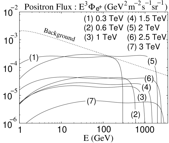
Figure 3: (Interstellar) positron flux from the wino-like neutralino annihilation. The signal fluxes for the wino mass $m=0.3$, 0.6, 1, 1.5, 2, 2.5, and 3 TeV are shown as solid lines. The expected background flux of positrons from the cosmic ray simulation is also shown as a dotted line.

First, we show the positron flux from the wino-like neutralino annihilation in Fig. 3. In this figure, the signal flux is shown as solid lines. The wino mass is taken to be $m=0.3$, 0.6, 1, 1.5, 2, 2.5, and 3 TeV. For comparison, the expected background flux of positrons from the cosmic ray simulation is also shown as a dotted line. The effect of the solar modulation is not included, and thus the spectrums below 10 GeV have uncertainties. However, since the high-energy positron spectrum is important for the discrimination of the signal from the background as indicated in Fig. 3, the uncertainties from the solar modulation are not serious.

When the wino mass is around 300 GeV, the signal flux is comparable to the background flux in the energy range 100 GeV$\mathop{}_{\textstyle\sim}^{\textstyle<}E\mathop{}_{\textstyle\sim}^{\textstyle<}$ 300 GeV. Furthermore, the signal flux for the mass around 2 TeV also exceeds the background one in the energy range $E\gtrsim 100$ GeV. The latter comes from the resonant DM annihilation. It is also noticed that a bump appears in each signal spectrum at around $m/2$. The positrons with energy above the bump come from the direct decay of weak gauge bosons, while those with energy below the bump are produced mainly by the hadronic cascade decay of the gauge bosons.

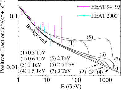
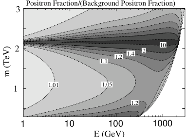
Figure 4: (Left figure) Positron fraction, $e^{+}/(e^{+}+e^{-})$, as a function of positron energy $E$ in the wino-like neutralino DM. For comparison, the expected background positron fraction, the positron data HEAT 94-95 and HEAT 2000 are also shown in this figure. (Right figure) Contour plot of the ratio between the positron fractions including positrons from the DM annihilation and without it (that is the background positron fraction) in a $(E,m)$ plane.

Next, we consider the positron fraction calculated from the positron flux in the Fig. 3 and the expected background ones in Eqs. (10). The result is shown in Fig. 4. In the left figure, the positron fraction is depicted as a function of positron energy for several wino masses. The choice of the mass is the same as that in the Fig. 3. The expected background positron fraction, the positron data HEAT 94-95 [12] and HEAT 2000 [24] are also shown in this figure. In the right figure of Fig. 4, the ratio of the fraction including positrons from the DM annihilation to the background one is depicted as a contour plot in a $(E,m)$ plane. From these figures, it is clear that the signature becomes more significant for high-energy positrons. In particular, there is a large difference between the expected signal and the background when the wino mass is a few hundred GeV or around 2 TeV.

Here, we address the HEAT experiment [12, 24], which reported the positron excess from the expected background. The spectrum of the observed fraction is almost flat around 0.06 in a energy range 4 GeV $\lesssim E\lesssim$ 20 GeV. The positron fractions for both $m=300$ GeV and $2$ TeV in the figure are consistent with it within the experimental error.

In addition, the effect of the inhomogeneity in the local DM distribution on the positron flux is recently discussed, whose existence is supported by the $N$-bodies simulations. In these arguments, the positron flux from the DM annihilation is enhanced if there are clumps of the DM in the vicinity of the solar system. The effect is parametrized as a boost factor ($BF$) [25], which is defined by a ratio of the signal fluxes with inhomogeneity and without inhomogeneity. The boost factor may reach $\sim$ 5 when the inhomogeneity exists, while the factor is equal to one if the DM is distributed homogeneously. Thus, the wino-like neutralino with the mass $\sim$ 300 GeV or 2 TeV can explain the HEAT result quite naturally. It is amazing that the wino-like neutralino with 2 TeV naturally accounts for not only the DM abundance thermally but also the HEAT anomaly.

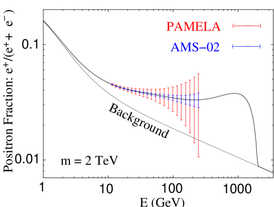
Figure 5: Sensitivities of the upcoming experiments. The positron fraction, $e^{+}/(e^{+}+e^{-})$, for $m=2$ TeV and that of the background are shown as solid and dotted lines, respectively. The error bars in the figure correspond to the statistical errors projected for the PAMELA and AMS-02 experiments after three years of observations.

Next, we discuss the potential of the upcoming PAMELA [10] and AMS-02 [11] experiments, which have good sensitivities in a broad region of positron energy 10 GeV $\lesssim E\lesssim$ 270 GeV, might detect the signal from the wino-like neutralino DM annihilation. We estimate the sensitivities of those experiments following the method in Ref. [27]. In Fig. 5, we show the sensitivities of the PAMELA and AMS-02. The positron fraction, $e^{+}/(e^{+}+e^{-})$, for $m=2$ TeV and that of the background are shown as solid and dotted lines, respectively. The error bars in the figure correspond to the statistical errors projected for the PAMELA and AMS-02 experiments after three years of observations. As shown in this figure, positrons with energy of some tens of GeV will be clearly discriminated from the background.

Finally, we discuss other uncertainties of the signal flux. First, in the case of the positron propagation with high energy, we do not have to worry about uncertainties from the thickness of the tangled magnetic field ($L$). This is because high-energy positrons we observe are produced within a few kpc around the solar system. Positrons far from the earth lose their energies during the propagation, and consequently they contribute to the low-energy part of the flux. The distance in which positrons travel without significant energy loss is typically

$$r \simeq \sqrt{\frac{K(E)E}{b(E)}}=1.7\times\left(E/{\rm 100~{}GeV}\right)^{-0.27}~{}({\rm kpc})~{}.$$ (11)

Thus, the positron flux at high energy does not suffer from the uncertainties of the thickness $L$ (because $L\gtrsim$ a few kpc).

Second is the DM distribution in the halo. We have assumed the isothermal halo in Eq. (5) in the above. Various DM halo models are proposed from the $N$-bodies simulations, however, the high-energy positron flux from the DM annihilation is considered to be almost independent of the choice of the halo model. The main difference among the halo models appears in the galactic center. However, the high-energy positrons produced around the galactic center can not reach to the earth, and the positron flux has little ambiguity from it around the solar system.

4 Antiproton signature from wino-like dark matter annihilation

The antiproton flux from the wino-like neutralino DM annihilation is discussed in this section. The method for calculation of the flux is essentially the same as that of the positron flux. First, the antiproton injection in the galactic halo (source term) and the propagation of the antiprotons are discussed, and the antiproton flux from the wino-like neutralino annihilation in the galactic halo is evaluated. The antiproton background originated from the cosmic rays is also discussed.

4.1 Production rate of antiprotons from dark matter annihilation

Antiprotons from the wino-like neutralino annihilation are also produced through the cascade decay of weak gauge bosons. The difference between the antiproton and the positron production rates (source terms) appears only in the fragmentation functions, and then the antiproton production rate is given as

$$Q(T,\vec{r})=\frac{1}{2}n^{2}(\vec{r})\sum_{f}\langle\sigma v\rangle_{f}\left(\frac{dN_{\bar{p}}}{dT}\right)_{f}~{}.$$ (12)

where $T(\equiv E-m)$ is the kinetic energy of antiproton and $(dN_{\bar{p}}/dT)_{f}$ is the fragmentation function.

	$j=1$	$j=2$	$j=3$	$j=4$
$i=1$	306.0	0.28	7.2$\times 10^{-4}$	2.25
$i=2$	2.32	0.05	0	0
$i=3$	-8.5	-0.31	0	0
$i=4$	-0.39	-0.17	$-2.0\times 10^{-2}$	0.23

	$j=1$	$j=2$	$j=3$	$j=4$
$i=1$	480.0	0.26	9.6$\times 10^{-4}$	2.27
$i=2$	2.17	0.05	0	0
$i=3$	-8.5	-0.31	0	0
$i=4$	-0.33	-0.075	$-1.5\times 10^{-4}$	0.71

Table 1: Coefficients in Eq. (14), $a_{ij},$ for $W^{+}W^{-}$ process (left panel) and $ZZ$ one (right panel).

As in the case of the fragmentation functions for positrons, the functions for antiprotons are calculated from the Monte-Carlo simulation. In this paper, we use the simple parametrization in Ref. [28] which fits the result of the PYTHIA Monte-Carlo code [29],

$$\left(\frac{dN_{\bar{p}}}{dx}\right)_{f}=\left(p_{1}x^{p_{3}}+p_{2}|\log_{10}x|^{p_{4}}\right)^{-1}~{},$$ (13)

where $x=T/m$. The parameters $p_{i}$ in the above equation depend on the neutralino mass in addition to the annihilation channels, and they are given as

$$p_{i}(m)=\left(a_{i1}m^{a_{i2}}+a_{i3}m^{a_{i4}}\right)^{-1}~{}.$$ (14)

The values of the coefficients, $a_{ij}$, are listed in Table 1 for the $W^{+}W^{-}$ process (left panel) and the $ZZ$ one (right panel). The parametrization for the fragmentation functions is valid for the neutralino mass in the range (50 – 5000) GeV. We dropped quark processes such as $t\bar{t}$ and $b\bar{b}$ since the annihilation cross sections are very small due to heavy squark masses and helicity suppression.

4.2 Propagation of antiprotons in the galaxy

In order to treat the propagation of antiprotons, we use the diffusion model as in the case of positrons. The diffusion equation describing the propagation is written as

$$K_{p}(T)\nabla^{2}f_{\bar{p}}(T,\vec{r})-\frac{\partial}{\partial z}\left(V_{C}(z)f_{\bar{p}}(T,\vec{r})\right)-2h\delta(z)\Gamma_{\rm ann}f_{\bar{p}}(T,\vec{r})$$

$$+Q(T,\vec{r})+Q^{\rm tert}(T,\vec{r}) = 0~{},$$ (15)

where $f_{\bar{p}}(T,\vec{r})$ is the number density of antiprotons per unit energy. The steady state condition ($\partial f_{\bar{p}}/\partial t=0$) is assumed as discussed in the positron case. For the evaluation of the equation, we use the cylinder coordinate. The interaction of antiproton with matter is confined on the galactic plane, which is expressed as the infinitely thin disk with radius $R=20$ kpc at the $z=0$. The diffusive halo is the cylinder with radius $R=20$ kpc and the half-height $L$. The boundary condition for solving the equation is taken to be the same as the positron case.

The diffusion equation (15) is essentially the same as that in Eq. (6). However, there are some differences, for example, the energy-loss term does not appear in Eq. (15). This is because protons are much heavier than electrons, so that we can neglect the energy-loss due to the scattering with background photons. The other differences are the term related to the convective wind (second term), the interaction term with matter in the galactic plane (third term) and the tertiary antiproton term (last term). These three terms are not so important when we consider the antiproton flux with high energy ($T\gtrsim$ a few GeV). We include these terms in the diffusion equation for completeness.

The diffusion coefficient $K_{p}$ is determined by the Boron to Carbon ratio $B/C$ in the cosmic rays, which is the same as the positron case. For the calculation of the antiproton flux, we parametrize the diffusion constant as Refs. [30, 31],

$$K_{p}(\mathcal{R})=K_{0}\beta\mathcal{R}^{\delta}~{},$$ (16)

where the diffusion coefficient is assumed to be constant within the diffusion zone. The variable $\mathcal{R}$ is called the rigidity, which is defined by the momentum of the particle per unit charge $\mathcal{R}\equiv p/Z$. For the values of $\delta$ and $K_{0}$, we use the parameter sets in Table 2. These values are favored from the $B/C$ analysis [32].

case	$\delta$	$K_{0}$(kpc2/Myr)	$L$ (kpc)	$V_{c}$(km/s)
max	0.46	0.0765	15	5
med	0.70	0.0112	4	12
min	0.85	0.0016	1	13.5

Table 2: Astrophysical parameters compatible with the $B/C$ analysis [32]. Three cases give the maximal, median and minimal signal antiproton fluxes.

The second term in Eq. (15), $\partial(V_{C}(z)f_{\bar{p}})/\partial z$, is not included in the equation for the positron flux. This term is related to the convective wind, which represents the movement of medium responsible for the diffusion. The direction of the wind is assumed to be perpendicular to the disc plane, and the velocity $V_{C}(z)$ is constant throughout the diffusive volume,

$$V_{C}(z)=\left(2\theta(z)-1\right)V_{c}~{},$$ (17)

where the value for $V_{c}$ is given in Table 2.

Next one is the third term in Eq. (15), $-2h\delta(z)\Gamma_{\rm ann}f_{\bar{p}}$, which represents the annihilation between antiproton and interstellar proton in the galactic plane. The parameter $h$ in the term is the half-height of disk and set to be 100 pc $(\ll L)$, while $\Gamma_{\rm ann}$ is the annihilation rate between antiproton and proton,

$$\Gamma_{\rm ann}=(n_{\rm H}+4^{2/3}n_{\rm He})\sigma^{\rm ann}_{\bar{p}p}v_{\bar{p}}~{},$$ (18)

where $v_{\bar{p}}$ is the velocity of antiproton, $n_{\rm H}$ denotes the hydrogen number density ($\sim$ 1 cm^-3), and $n_{\rm He}$ is the helium number density which we assume to be 7% of $n_{\rm H}$ [33]. The factor $4^{2/3}$ arises from a geometrical approximation [34]. The annihilation cross section between antiproton and proton, $\sigma^{\rm ann}_{\bar{p}p}$, is given by [35, 36]

$$\sigma^{\rm ann}_{\bar{p}p}(T)=\left\{\begin{array}[]{ll}661\left(1+0.0115~{}T^{-0.774}-0.948~{}T^{0.0151}\right)~{}{\rm mb}~{},&T<15.5{\rm~{}GeV}~{},\\ 36~{}T^{-0.5}~{}{\rm mb}~{},&T\geq 15.5~{}{\rm GeV}~{},\\ \end{array}\right.$$ (21)

where $T$ is in unit of GeV. This interaction dominates over inelastic interactions at low energy. Hence, the flux of antiprotons with low energy is decreased by the annihilation.

For higher energy antiprotons ($T\gtrsim 10$ GeV), the inelastic interaction is not dominated by annihilation, however, the non-annihilating scattering is important. The interaction lowers energies of antiprotons, $T^{\prime}$ to $T(<T^{\prime})$. These antiprotons are called tertiary antiprotons. We include this effect in $Q^{\rm tert}(T,\vec{r})$, which is given by

$$Q^{\rm tert}(T,\vec{r}) = (n_{\rm H}+4^{2/3}n_{\rm He})$$ (22)

$$\times\left[\int_{T}^{m}\frac{\sigma_{\bar{p}p}^{\rm non-ann}(T^{\prime})}{T^{\prime}}v^{\prime}_{\bar{p}}f_{\bar{p}}(T^{\prime},\vec{r})dT^{\prime}-\sigma_{\bar{p}p}^{\rm non-ann}(T)v_{\bar{p}}f_{\bar{p}}(T,\vec{r})\right].$$

The first term in the bracket is the contribution to the antiproton flux with energy $T$ from the inelastic scattering of antiprotons with energy larger than $T$, while the second term compensates it so that the total antiproton number is not changed in this process. Here, $\sigma_{\bar{p}p}^{\rm non-ann}(T)$ is given as the difference between the total inelastic cross section $\sigma_{\bar{p}p}^{\rm inel}$ and the annihilation cross section $\sigma_{\bar{p}p}^{\rm ann}$. The total inelastic cross section is given in Ref. [35] as

$$\sigma^{\rm inel}_{\bar{p}p}(T)=24.7\left(1+0.584T^{-0.115}+0.856T^{-0.566}\right)~{}~{}({\rm mb})~{},$$ (23)

where $T$ is in unit of GeV.

The number density of antiprotons $f_{\bar{p}}$ is obtained by solving the diffusion equation (15). We can solve this equation full-analytically [22, 30]. The detailed expression of the solution is presented in Appendix B. After solving the equation for the number density, the interstellar flux of antiprotons from the DM annihilation in the vicinity of the solar system is obtained as

$$\Phi_{\rm IS}=\frac{v_{\bar{p}}}{4\pi}f_{\bar{p}}(T,\vec{r}_{\odot}).$$ (24)

Here, we discuss the effect of the solar modulation on the antiproton flux. This is important for antiprotons with low kinetic energies ($\lesssim$ 3 GeV). Using the force field approximation, the flux of antiprotons on the top of atmosphere $\Phi_{\rm TOA}$ is obtained from the interstellar flux $\Phi_{\rm IS}$ as

$$\frac{\Phi_{\rm TOA}(T^{\rm TOA})}{\Phi_{\rm IS}(T^{\rm IS})}=\left(\frac{p^{\rm TOA}}{p^{\rm IS}}\right)^{2}~{},\qquad T^{\rm TOA}=T^{\rm IS}-|Z|\phi~{},$$ (25)

where $p^{\rm TOA}(T^{\rm TOA})$ and $p^{\rm IS}(T^{\rm IS})$ are momentums (kinetic energies) of antiproton on the top of the atmosphere and in the interstellar, respectively. The solar modulation parameter $\phi$ varies according to the 11 years solar cycle. This parameter takes a value from about 500 MV at the minimum solar activity to 1.3 GV at the maximum solar activity. Larger $\phi$ lowers the antiprotons flux on the top of atmosphere flux at low energy.

4.3 Background flux of antiprotons

In this section, we discuss the antiproton background flux. The antiprotons are produced as the secondary products of cosmic rays by the nuclear reaction with the interstellar gas in the galactic disk. The main contribution to the antiproton flux comes from the collision between the cosmic ray protons and the interstellar hydrogen gas. Again, the production phenomena are described by the diffusion equation. We solve the diffusion equation and calculate the background flux. Since the concrete formalism for obtaining the flux is very complex, we mention only the strategy for the calculation here. The antiproton background is also discussed in Refs. [28, 34, 37].

While the interstellar primary proton flux is required to evaluate the background antiproton flux, it is impossible to measure it directly. However, it is obtained by solving the diffusion equation under an assumption of the source function. The primary protons are believed to be produced by supernovae. Hence, the proton source term with a few undetermined parameters is assumed, and the interstellar proton flux is obtained by solving the diffusion equation with this source term. In this case, the parameters in the source term are fixed by comparing the evaluated flux with the observed cosmic rays on the earth in the measurements such as BESS [38] and AMS [39]. The fitting function for the primary proton flux derived as above is given in Ref. [34]. We use it in our evaluation of the background antiproton flux.

Next, the antiproton flux is evaluated from the primary proton flux by solving the corresponding diffusion equation. The equation is the same as that in Eq. (15) except for the source term. Since the antiprotons are produced by the nuclear reaction between the cosmic rays and interstellar gas, the source term is given by the proton flux and the cross sections for the reactions.

The antiprotons are dominantly produced by the process $p+{\rm H}\rightarrow\bar{p}+{\rm X}$. In the rest frame of the hydrogen atom, the kinetic energy threshold for the incident proton to produce secondary antiprotons is $6m_{p}$. Furthermore, the number density of the incident proton decreases as energy increases. As a result, the spectrum of antiprotons from this process has a peak at a few GeV. In addition to this process, we include the inelastic collision between proton and helium, $p+{\rm He}\rightarrow\bar{p}+{\rm X}$, for generating the secondary antiprotons. The process with the helium contributes to the antiproton flux sub-dominantly in the most energy range. However, the antiprotons from the process are a dominant component at low energy with the tertiary antiprotons ($T\lesssim$ 0.1 GeV). Thus, the source term for the secondary antiproton turns out to be

$$Q(T)=2\int_{T_{\rm th}}^{\infty}dT^{\prime}4\pi\Phi_{p}^{\rm(prim)}(T^{\prime})\left[n_{\rm H}\frac{d\sigma_{p{\rm H}\rightarrow\bar{p}X}}{dT^{\prime}}(T^{\prime},T)+n_{\rm He}\frac{d\sigma_{p{\rm He}\rightarrow\bar{p}X}}{dT^{\prime}}(T^{\prime},T)\right]~{}.$$ (26)

The factor 2 comes from the fact that the antiprotons are produced from the antineutron decay in addition to the direct production of antiprotons. The threshold energy $T_{\rm th}$ is $6m_{p}$ and $\Phi_{p}^{\rm(prim)}$ is the proton flux. The differential cross section ${d\sigma}(T^{\prime},T)/{dT^{\prime}}$ is for the production of an antiproton with energy $T$ from an incident proton of energy $T^{\prime}$. The cross sections are given in Ref. [40].

Within uncertainties of the observations, the obtained flux for the antiproton background is consistent with the results by BESS [41], AMS [42] and CAPRICE [43], which observe the low-energy antiprotons ((0.2-50) GeV). We use the background flux for estimating the antiproton signature from the DM annihilation.

4.4 Antiproton signature from dark matter annihilation

Now we are in a position to discuss the antiproton signature from the wino-like neutralino annihilation in the galactic halo. We calculate the antiproton flux from the neutralino annihilation by solving Eq. (15), and compare the result with the background flux discussed in the previous section.

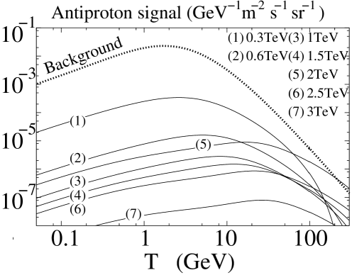
Figure 6: Antiproton flux from the wino-like neutralino annihilation on the top of atmosphere as a function of antiproton kinetic energy. The wino mass is taken to be $m=0.3$, 0.6, 1, 1.5, 2, 2.5, and 3 TeV. The solar modulation parameter $\phi$ is set to be 500 MV. For comparison, the background flux is depicted as a dotted line.

In Fig. 6, the flux of the antiproton signal on the top of the atmosphere is depicted for various wino masses as a function of the antiproton kinetic energy. In this figure, we use the astrophysical parameters of the median set in Table 2, which gives the minimal $\chi^{2}$ for the $B/C$ analysis [32]. The parameter of solar modulation $\phi$ is set to be 500 MV, which corresponds to almost minimum solar activity. For comparison, the background flux is also shown as a dotted line. As shown in this figure, it is implausible to exceed the background for almost all region of the wino mass. The exception is only the case of the wino mass around 2 TeV. In this case, the wino-like neutralinos annihilate resonantly as discussed in section 2, and the signal flux is almost comparable to the background flux at high energy ($T\gtrsim 100$ GeV).

Figure 7: Antiproton flux from the wino-like neutralino annihilation and the background flux on the top of atmosphere for three astrophysical parameter sets in Table 2. Here, we take the wino mass 2 TeV. The solar modulation parameter $\phi$ is set to be 500 MV as in the previous figure.

Let us discuss the uncertainties in the prediction of the signal antiproton flux. In Fig. 7 we show the signal antiproton and the background fluxes on the top of atmosphere for three astrophysical parameter sets in Table 2, in order to see the dependence on choice of astrophysical parameter sets. Here, we take the wino mass 2 TeV and the solar modulation parameter is 500 MV.

The uncertainties in the astrophysical parameters lead to an uncertainty of a factor $O(100)$ for the prediction of the signal antiproton flux. The flux from the neutralino annihilation depends strongly on the astrophysical parameters, especially, the value of the thickness of the diffusion zone $L$. A larger $L$ means more injection of signal antiprotons and leads to larger signal flux. On the other hand, the background flux has no strong sensitivity to $L$, as shown in the figure. As a result, we can observe the signal antiprotons only when $L$ is large enough. The situation is very different from the positron signal, in which only the DM within a few kpc contributes to the flux due to the rapid energy loss of high-energy electrons.

Other uncertainties come from the choice of the DM halo profile. The signal antiprotons in the cosmic rays can travel far from the solar system, while the positrons are originated within a few kpc. Therefore, the prediction of the signal antiproton flux varies with uncertainties in the halo profile [28, 32]. This uncertainties depend on the size of diffusive halo, especially $L$. For large $L(\simeq 15$ kpc) the antiproton flux from the neutralino annihilation may be changed by several tens of percent depending on the choice of halo profile. However, for moderate value of $L\lesssim 5$ kpc, the uncertainties of halo profile is negligible with respect to other ones such as the diffusive halo size.

Finally, we concentrate the issue of discrimination of the signal from the background. We showed that the wino-like neutralino annihilation with mass around 2 TeV leads to the signal antiproton flux comparable to or larger than the background one. In this case, a bump appears in the antiproton spectrum. However, it might be still difficult to recognize presence of the bump from the observed antiproton spectrum in the upcoming experiments such as PAMELA and AMS-02, compared with cases of the positron flux from the DM annihilation.

The positron flux has a high-energy component, which is produced more directly from the leptonic weak boson decays, so that the signal-background ratio for the higher energy positron flux is better. However, since the spectrum of the signal antiproton flux is featureless even at high energy, it suffers more from uncertainties of the background.

The background antiprotons at high-energy mainly come from the interaction of the primary protons in the cosmic rays as discussed in the previous section. The proton spectrum is mainly determined by the source term, that is, the injection from supernovae. The high-energy protons are produced by the shock-wave acceleration. It implies that the spectrum shows the power-law behavior in terms of the energy. However, it is difficult to predict the slope of the power law. Thus, the background flux also has an ambiguity in the slope at a high-energy range. Varying the slope at the source term is immediately reflected to the slope of the antiproton flux at the earth. As a result, with lack of the knowledge of the slope of the source term, it is difficult to distinguish the signal from the background using only the slope of spectrum.

It may be important to observe the antiprotons with energy around the neutralino mass so that the bump may be recognized. When the wino mass is around 300 GeV and the thickness of the diffusion zone $L$ is large, the whole structure of the bump might be figured out in the experiments. However, when the mass is around 2 TeV, it would be a hard job to detect antiprotons with such a high energy.

5 Conclusions

In this article, we have studied indirect detection of the wino-like neutralino DM using cosmic ray positron and antiproton observations. Non-perturbative effect enhances the neutralino annihilation cross section when the mass is larger than about 1 TeV. Especially, when the mass is around 2 TeV, the cross section is enhanced significantly due to the resonance effect of the bound state, which is composed of the wino-like neutralinos and charginos. In those cases, the cosmic ray positron and antiproton fluxes produced by the neutralino annihilation in the galactic halo also enhance, and the sensitivities of the upcoming experiments, such as PAMELA and AMS-02, are improved for the heavier neutralino DM. It is noticed that the relic abundance of the wino-like neutralino in the universe is explained by the thermal scenario when the mass is around 2 TeV. It might be difficult to study such a heavy neutralinos in experiments except for observation of the cosmic rays. Even in the direct DM detection, the sensitivity should cover $10^{-(46-47)}$cm² for the spin-independent cross section so that the heavy wino-like neutralino is detected [44]. We have concentrated mainly the heavy wino-like neutralino and have evaluated the positron and antiproton fluxes from the neutralino annihilation using the diffusion model.

We found that both positron and antiproton fluxes increase significantly around the resonance ($m\sim 2$ TeV). However, the positron flux measurement has more prospects to detect the heavy wino-like neutralino DM, compared with the antiproton one. The signal positron flux exceeds the expected background for the positron energy larger than about 100 GeV, and the spectrums in the positron flux and the positron fraction are significantly deviated from the background ones. In addition, it is plausible that the signal positron spectrum at high energy is less sensitive to the astrophysical parameters in the diffusion model or the DM halo profile, since the positrons we observe are produced within a few kpc around the solar system. PAMELA and AMS-02 have good sensitivities in a broad region of the positron energy 10 GeV $\lesssim E\lesssim$ 270 GeV. Thus, they may distinguish whether the heavy wino-like neutralino is the DM.

We have also discussed the HEAT anomaly in a positron energy range 4 GeV $\lesssim E\lesssim$ 20 GeV. The positron flux from the heavy wino-like neutralino annihilation with mass 2 TeV is consistent with it within the experimental error. It is amazing that the wino-like neutralino can explain both the DM relic abundance and the HEAT anomaly even when the mass is around 2 TeV.

The antiproton flux from the wino-like neutralino annihilation may be comparable to or larger than the expected background for the mass around 2 TeV. However, it is strongly dependent on the astrophysical parameters in the diffusion model. In addition to it, it might be difficult to discriminate the signal from the background, since the antiproton spectrum is featureless.

Appendix A: Solution of diffusion equation for positron signal

Here we show how to solve the diffusion equation for the positron signal from the DM annihilation. With use of dimensionless parameter $\epsilon=(E/$ 1GeV), the equation (6) is rewritten under the steady state condition as

$$K(\epsilon)\nabla^{2}f_{e^{+}}(\epsilon,r,z)+\frac{\partial}{\partial\epsilon}\left(b(\epsilon)f_{e^{+}}(\epsilon,r,z)\right)+Q(\epsilon,r,z)=0~{},$$ (27)

where $K(\epsilon)=K_{0}(C+\epsilon^{\alpha})$ and $b(\epsilon)=\epsilon^{2}/\tau$. The values for $K_{0}$, $C$, $\alpha$, and $\tau$ can be read off in text.

We use the cylinder coordinate, so the differentiation $\nabla^{2}$ is written as $\nabla^{2}=\partial^{2}_{r}+r^{-1}\partial_{r}+\partial_{z}^{2}$. The source term $Q(\epsilon,r,z)$ including the information of the DM annihilation is

$$Q(\epsilon,r,z)=\frac{1}{2}\left({n(r,z)}\right)^{2}\sum_{f}\langle\sigma v\rangle_{f}\left(\frac{dN_{e^{+}}}{d\epsilon}\right)_{f}~{},$$ (28)

where $f$ means the final state of the DM annihilation and $(dN_{e^{+}}/d\epsilon)_{f}$ is the fragmentation function for the final state $f$. We impose the boundary condition so that the density of positron $f_{e^{+}}(\epsilon,r,z)$ becomes zero at the surface of the diffusion zone, which is given by a cylinder with radius $R$ and half-height $L$.

Due to the boundary condition, it is convenient to expand the density by the zeroth-order Bessel function $J_{0}$ for the coordinate $r$ and by a sine function for $z$,

$$f_{e^{+}}(\epsilon,r,z)=\sum_{m,n=1}^{\infty}A_{n,m}(\epsilon)J_{0}\left(\frac{\zeta_{n}}{R}r\right)\sin\left(\frac{m\pi}{2L}(z-L)\right)~{},$$ (29)

where $\zeta_{n}$ are successive zeros of the function $J_{0}$. Using the expansion, it is obvious that the density satisfies the boundary condition above.

We comment on the some properties of the Bessel function $J_{0}$ here. It satisfies a following differential equation,

$$\frac{d^{2}}{dr^{2}}J_{0}\left(\frac{\zeta_{n}}{R}r\right)+\frac{1}{r}\frac{d}{dr}J_{0}\left(\frac{\zeta_{n}}{R}r\right)+\frac{\zeta_{n}^{2}}{R^{2}}J_{0}\left(\frac{\zeta_{n}}{R}r\right)=0~{},$$ (30)

and has a following orthogonal relation

$$\int_{0}^{R}rdrJ_{0}\left(\frac{\zeta_{i}}{R}r\right)J_{0}\left(\frac{\zeta_{j}}{R}r\right)=\frac{1}{2}J_{1}^{2}(\zeta_{i})R^{2}\delta_{ij}~{},$$ (31)

where $J_{1}$ is the first-order Bessel function.

Substituting Eq. (29) into the diffusion equation and using the differential equation and orthogonal relation above, we obtain

$$\frac{dA_{n,m}}{d\epsilon}+\frac{2}{\epsilon}A_{n,m}-\left(\frac{\zeta_{n}^{2}}{R^{2}}+\frac{m^{2}\pi^{2}}{4L^{2}}\right)\frac{K_{0}\tau(C+\epsilon^{\alpha})}{\epsilon^{2}}A_{n,m}=-\frac{\tau}{\epsilon^{2}}Q_{n,m}(\epsilon)~{}.$$ (32)

Here, we also expand the source term $Q$ by the Bessel and sine functions, and the coefficients of the expansion $Q_{n,m}$ are written

$$Q_{n,m}(\epsilon)=\frac{2}{J_{1}^{2}(\zeta_{n})R^{2}L}\int_{0}^{R}rdr\int_{-L}^{L}dzQ(r,z,\epsilon)J_{0}\left(\frac{\zeta_{n}}{R}r\right)\sin\left(\frac{m\pi}{2L}(z-L)\right)~{}.$$ (33)

The boundary condition for $A_{n,m}$ is given by $A_{n,m}(\epsilon_{\rm max})=0$, where $\epsilon_{\rm max}\equiv{\rm max}\left({\rm supp}(Q_{n,m})\right)(\sim m)$. The condition means that $A_{n,m}(\epsilon)=0$ if $\epsilon\geq\epsilon_{\rm max}$. The function $A_{n,m}(\epsilon)$ must be a continuous function of $\epsilon$. Solving Eq. (32), we obtain

$$A_{n,m} = \int_{\epsilon}^{\epsilon_{\rm max}}d\epsilon^{\prime}\tau Q_{n,m}(\epsilon^{\prime})\frac{1}{\epsilon^{2}}$$ (34)

$$\times\exp\left[\left(\frac{\zeta_{n}^{2}}{R^{2}}+\frac{m^{2}\pi^{2}}{4L^{2}}\right)K_{0}\tau\left(-\frac{C}{\epsilon}+\frac{C}{\epsilon^{\prime}}+\frac{\epsilon^{\alpha-1}}{\alpha-1}-\frac{(\epsilon^{\prime})^{\alpha-1}}{\alpha-1}\right)\right]~{}.$$

Substituting $A_{n,m}$ into Eq. (29), we obtain the number density $f_{e^{+}}(\epsilon,r,z)$.

Appendix B: Solution of diffusion equation for antiproton signal

The strategy of solving the diffusion equation for the antiproton signal in Eq. (15) is essentially the same as that in the positron case. In the equation, the term representing the energy loss of the particles, which has differentiation with respect to $T$, is absent. It makes it much easier to solve the equation than that of positrons. Thus, we show only the result here. For more detailed calculations, see Refs. [22, 30].

The number density of antiprotons at the solar system, $f_{\bar{p}}(T,\vec{r}_{\odot})$, is given by

$$f_{\bar{p}}(T,\vec{r}_{\odot}) = \sum_{i=1}^{\infty}\exp\left(-\frac{V_{c}L}{2K}\right)\frac{y_{i}(L)}{A_{i}\sinh(S_{i}L/2)}J_{0}\left(\zeta_{i}\frac{r}{R}\right)~{},$$

$$y_{i}(z) = 2\int_{0}^{z}dz^{\prime}\exp\left(\frac{V_{c}(z-z^{\prime})}{2K}\right)\sinh\left(\frac{S_{i}(z-z^{\prime})}{2}\right)Q_{i}(T,z^{\prime})~{},$$ (35)

where $Q_{i}$ is the coefficient of the expansion of the source term $Q(T,r,z)$ by the Bessel function,

$$Q(T,r,z)=\sum_{i=1}^{\infty}Q_{i}(T,z)J_{0}\left(\zeta_{i}\frac{r}{R}\right)~{}.$$ (36)

The parameter $A_{i}$ in Eq. (35) includes the information about the propagation of antiprotons, and it is given as

$$A_{i}=2h\Gamma_{\rm inel}+V_{c}+KS_{i}\coth\left(\frac{S_{i}L}{2}\right)~{},\qquad S_{i}=\sqrt{\left(\frac{4\zeta_{i}^{2}}{R^{2}}+\frac{V_{c}^{2}}{K^{2}}\right)}~{}.$$ (37)

From this solution, we can derive the simple relation between the source term and the density. Assuming that the source term scales as $Q\propto E^{-\alpha}$, the number density behaves as $f_{\bar{p}}(T,\vec{r}_{\odot})\propto E^{-\alpha-\delta}$, because of $A_{i}\propto K(E)\propto E^{\delta}$.

References

- [1] D. N. Spergel et al. [WMAP Collaboration], Astrophys. J. Suppl. 148, 175 (2003).
- [2] C. L. Bennett et al., Astrophys. J. Suppl. 148, 1 (2003).
- [3] G. Jungman, M. Kamionkowski and K. Griest, Phys. Rept. 267, 195 (1996); L. Bergstrom, Rept. Prog. Phys. 63, 793 (2000); G. Bertone, D. Hooper and J. Silk, Phys. Rept. 405, 279 (2005); C. Munoz, Int. J. Mod. Phys. A 19, 3093 (2004).
- [4] H. P. Nilles, Phys. Rept. 110, 1 (1984); H. E. Haber and G. L. Kane, Phys. Rept. 117, 75 (1985).
- [5] L. Randall and R. Sundrum, Nucl. Phys. B 557, 79 (1999); G. F. Giudice, M. A. Luty, H. Murayama and R. Rattazzi, JHEP 9812, 027 (1998).
- [6] M. W. Goodman and E. Witten, Phys. Rev. D 31, 3059 (1985).
- [7] J. Hisano, S. Matsumoto and M. M. Nojiri, Phys. Rev. Lett. 92, 031303 (2004).
- [8] J. Hisano, S. Matsumoto, M. M. Nojiri and O. Saito, Phys. Rev. D 71, 063528 (2005).
- [9] S. Profumo and C. E. Yaguna, Phys. Rev. D 70, 095004 (2004).
- [10] M. Boezio et al., Nucl. Phys. Proc. Suppl. 134, 39 (2004).
- [11] F. Barao [AMS-02 Collaboration], Nucl. Instrum. Meth. A 535,134 (2004).
- [12] S. W. Barwick et al. [HEAT Collaboration], Astrophys. J. 482, L191 (1997).
- [13] J. Hisano, S. Matsumoto and M. M. Nojiri, Phys. Rev. D 67, 075014 (2003).
- [14] T. Moroi and L. Randall, Nucl. Phys. B 570, 455 (2000).
- [15] K. Kohri, M. Yamaguchi and J. Yokoyama, Phys. Rev. D 72, 083510 (2005).
- [16] K. Yamamoto, Phys. Lett. B 161, 289 (1985); ibid. B 168, 341 (1986); D. H. Lyth and E. D. Stewart, Phys. Rev. D 53, 1784 (1996).
- [17] G. Corcella et al., JHEP 0101, 010 (2001).
- [18] S. Rudaz and F. W. Stecker, Astrophys. J. 325, 16 (1988); M. Kamionkowski and M. S. Turner, Phys. Rev. D 43, 1774 (1991).
- [19] E. A. Baltz and J. Edsjo, Phys. Rev. D 59, 023511 (1999).
- [20] W. R. Webber, M. A. Lee and M. Gupta, Astrophys. J. 390, 96 (1992).
- [21] M. S. Longair, High-energy astrophysics, Vol. 2, Cambridge University Press, New York, 1994.
- [22] A. Barrau, G. Boudoul, F. Donato, D. Maurin, P. Salati and R. Taillet, Astron. Astrophys. 388, 676 (2002).
- [23] I. V. Moskalenko and A. W. Strong, Astrophys. J. 493, 694 (1998).
- [24] J. J. Beatty et al., Phys. Rev. Lett. 93, 241102 (2004).
- [25] The boost factor is discussed for example in Ref. [19] and the clumpy halo is discussed for example in Ref. [26].
- [26] J. Silk and A. Stebbins, Astrophys. J. 411, 439 (1993); L. Bergstrom, J. Edsjo, P. Gondolo and P. Ullio, Phys. Rev. D 59, 043506 (1999); V. Berezinsky, V. Dokuchaev and Y. Eroshenko, Phys. Rev. D 68, 103003 (2003).
- [27] D. Hooper and J. Silk, Phys. Rev. D 71, 083503 (2005).
- [28] L. Bergstrom, J. Edsjo and P. Ullio, Astrophys. J. 526, 215 (1999).
- [29] T. Sjostrand, Comput. Phys. Commun. 82, 74 (1994).
- [30] D. Maurin, R. Taillet, F. Donato, P. Salati, A. Barrau and G. Boudoul, arXiv:astro-ph/0212111.
- [31] D. Maurin, R. Taillet and F. Donato, Astron. Astrophys. 394, 1039 (2002).
- [32] F. Donato, N. Fornengo, D. Maurin, P. Salati and R. Taillet, Phys. Rev. D 69, 063501 (2004).
- [33] M. Garcia-Munoz, J. A. Simpson, T. G. Guzik, J. P. Wefel and S. H. Margolis, Astrophys. J. S64, 269 (1987).
- [34] F. Donato, D. Maurin, P. Salati, A. Barrau, G. Boudoul and R. Taillet, Astrophys. J. 563, 172 (2001).
- [35] L. C. Tan and L. K. Ng, J. Phys. G 9, 227 (1983).
- [36] R. J. Protheroe, Astrophys. J. 251, 387 (1981).
- [37] A. Bottino, F. Donato, N. Fornengo and P. Salati, Phys. Rev. D 58, 123503 (1998); A. Bottino, F. Donato, N. Fornengo and P. Salati, Phys. Rev. D 72, 083518 (2005).
- [38] T. Sanuki et al., Astrophys. J. 545, 1135 (2000).
- [39] J. Alcaraz et al. [AMS Collaboration], Phys. Lett. B 472, 215 (2000).
- [40] R. P. Duperray, C. Y. Huang, K. V. Protasov and M. Buenerd, Phys. Rev. D 68, 094017 (2003).
- [41] S. Orito et al. [BESS Collaboration], Phys. Rev. Lett. 84, 1078 (2000); T. Maeno et al. [BESS Collaboration], Astropart. Phys. 16, 121 (2001).
- [42] M. Aguilar et al. [AMS Collaboration], Phys. Rept. 366, 331 (2002) [Erratum-ibid. 380, 97 (2003)].
- [43] M. Boezio et al. [WiZard/CAPRICE Collaboration], Astrophys. J. 561, 787 (2001).
- [44] J. Hisano, S. Matsumoto, M. M. Nojiri and O. Saito, Phys. Rev. D 71, 015007 (2005).