High energy scattering in QCD: dipole approach with Pomeron loops
Abstract
In this talk we discuss the BFKL Pomeron Calculus and its interrelation with the colour dipole approach. The two key problems we consider are the probabilistic interpretation of the BFKL Pomeron Calculus and the possible scenario for the asymptotic behaviour of the scattering amplitude at high energy in QCD.
1 Introduction
The simplest approach that we can propose for high energy interaction is based [1, 2] on the BFKL Pomeron [3] and reggeon-like diagram technique for the BFKL Pomeron interactions [4, 5, 6, 7]. This technique which is a generalization of Gribov Reggeon Calculus [8], can be written in the elegant form of the functional integral (see Ref. [5] and the next section); and it is a challenge to solve this theory in QCD finding the high energy asymptotic behaviour. However, even this simple approach has not been solved during three decades of attempts by the high energy community. This failure stimulates a search for deeper understanding of physics which is behind the BFKL Pomeron Calculus. In particular, at the end of the Reggeon era it was understood [9, 10, 11] that the Reggeon Calculus can be reduced to a Markov process [12] for the probability of finding a given number of Pomerons at fixed rapidity . Such an interpretation, if it would be reasonable in QCD, can be useful, since it allows us to use powerful methods of statistical physics in our search for the solution.
The goal of this talk is to consider two main problems: the probabilistic interpretation of the BFKL Pomeron Calculus based on the idea that colour dipoles are the correct degrees of freedom at high energy QCD [13] and the possible solution for the scattering amplitude at high energy. Colourless dipoles play two different roles in our approach. First, they are partons (‘wee’ partons) for the BFKL Pomeron. This role is not related to the large approximation and, in principle, we can always speak about probability to find a definite number of dipoles instead of defining the probability to find a number of the BFKL Pomerons. The second role of the colour dipoles is that at high energies we can interpret the vertices of Pomeron merging and splitting in terms of the probability for two dipoles to annihilate in one dipole and of the probability for the decay of one dipole into two. It was shown in Ref. [13] that splitting can be described as the process of the dipole decay into two dipoles. However, the relation between the Pomeron merging () and the process of annihilation of two dipoles into one dipole is not so obvious and it will be discussed here.
Our presentation is based on Refs.[14, 15, 16, 17, 18] and we would like to thank Michael Lublinsky and Alex Prygarin for their contributions and for a great pleasure to work with them.
The outline of the talk looks as follows. In the next section we will discuss the BFKL Pomeron Calculus in the elegant form of the functional integral, suggested by M. Braun about five years ago [5]. We will show that the intensive recent work on this subject [19, 20, 16] confirms the BFKL Pomeron Calculus in spite of the fact that these attempts were based on slightly different but not more general assumptions.
In the third section the general approach based on the generating functional will be discussed. The set of equations for the amplitude of -dipole interaction with the target will be obtained and the interrelations between vertices of the Pomeron interactions and the microscopic dipole processes will be considered.
The fourth section is devoted to the toy model which simplifies the QCD interaction and allows us to see the main properties of high energy amplitude. In particular, we are going to discuss the solution of the equations for the asymptotic behaviour of the scattering amplitude at high energies.
In the fifth section we will consider a general case of QCD and will discuss the probabilistic interpretation as well as the scenario for the solution using the experience with the toy model.
In conclusion we are going to compare our approach with other approaches on the market.
2 The BFKL Pomeron Calculus
The main ingredient of this calculus is the Green function of the BFKL Pomeron describing the propagation of a pair of gluons from rapidity and points and to rapidity and points and 222Coordinates here are two dimensional vectors and, strictly speaking, should be denoted by or . However, we will use the notation hoping that it will not cause difficulties in understanding.. Since the Pomeron does not carry colour in the -channel, we can treat initial and final coordinates as coordinates of quark and antiquark in a colourless dipole. This Green function is well known[21] and has a form:
| (1) |
where vertices are given by
| (2) |
, 333 and are components of the two dimensional vector on -axis and - axis , ; and . The energy levels are the BFKL eigenvalues
| (3) |
where and is the Euler gamma function. and finally
| (4) |
The interaction between Pomerons is described by the triple Pomeron vertex which can be written in the coordinate representation [5] for the following process: two gluons with coordinates and at rapidity decay into two gluons pairs with coordinates and at rapidity and and at rapidity due to the Pomeron splitting at rapidity . It looks like
| (5) |
where
| (6) |
and the arrow shows the direction of action of the operator . For the inverse process of merging of two Pomerons into one we have
| (7) |
The theory with the interaction given by Eq. (5) and Eq. (7) can be written through the functional integral [5]
| (8) |
where describes free Pomerons, corresponds to their mutual interaction while relates to he interaction with the external sources (target and projectile). From Eq. (5) and Eq. (7) it is clear that
| (9) |
| (10) |
For we have local interaction both in rapidity and in coordinates, namely,
| (11) |
where ( stands for the projectile and target, respectively. The form of function depends on the non-perturbative input in our problem and for the case of nucleus target they are written in Ref. [5].
For the case of the projectile being a dipole that scatters off a nucleus the scattering amplitude has the form
| (12) |
where the extra comes from our normalization.
For further presentation we need some properties of the BFKL Green function [21]:
1. Generally,
| (13) |
| (14) |
2. The initial Green function () is equal to
| (15) |
3. It should be stressed that
| (16) |
4. In the sum of Eq. (1) only the term with is essential for the high energy asymptotic behaviour since all with are negative and, therefore, lead to contributions that decrease with energy. Taking into account only the first term, one can see that is the eigenfunction of operator , namely
| (17) | |||||
The last equation holds only approximately in the region where , but this is the most interesting region which is responsible for the high energy asymptotic behaviour of the scattering amplitude.
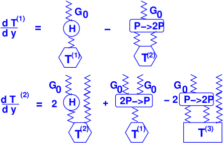
Using Eq. (5), Eq. (7) and Eq. (2) we can easily obtain the chain equation for multi-dipole amplitude noticing that every dipole interacts only with one Pomeron (see Eq. (12)). The equation is shown in Fig. (1) and it has the following form
| (18) |
| (19) |
Deriving Eq. (18) and Eq. (19) we use Eq. (15) and Eq. (16) as well as the normalization condition (see Eq. (12)) for the scattering amplitude. These two equations are the same as in Ref. [22]. This shows that in the papers [19, 22], actually, the same approach is developed as in the BFKL Pomeron Calculus (much later, of course), in spite of the fact that the authors think that they are doing something more general.
Assuming that , we obtain the Balitsky-Kovchegov equation [23, 24]. We can do this only if we can argue why the Pomeron splitting is more important than the Pomeron merging. For example this assumption is reasonable for the scattering of the dipole with the nucleus target. Generally speaking, the splitting and merging have the same order in ( see Eq. (5) and Eq. (7). In Eq. (18) and Eq. (19) these two processes look like having a different order of magnitude in but this fact does not interrelate with any physics and reflect only our normalization. However, we will see that for a probabilistic interpretation the correct normalization is very important.
Kernel is defined as
| (20) |
Function is equal to
| (21) |
where is given by Eq. (15) and we use the notation for a colourless pair of gluon (colour dipole).
3 Generating functional and probabilistic interpretation
In this section we discuss the main equations of the BFKL Pomeron Calculus in the formalism of the generating functional, which we consider as the most appropriate technique for the probabilistic interpretation of this approach top high energy scattering in QCD.
To begin with, let us write down the definition of the generating functional [13]
| (22) |
where is an arbitrary function of and . The coordinates describe the colorless pair of gluons or a dipole. is a probability density to find dipoles with the size , and with the impact parameter . It follows from the physical meaning of and the definition in Eq. (22) directly that the functional (Eq. (22)) obeys the condition
| (23) |
The physical meaning of this equation is that the sum over all probabilities is equal to unity.
Introducing vertices for the dipole process: (), () and ( we can write a typical birth-death equation in the form
| (24) |
| (27) | |||||
Multiplying this equation by the product and integrating over all and , we obtain the following linear equation for the generating functional:
| (28) |
with
| (29) |
| (30) | |||
| (31) |
Trying to make our presentation more transparent, we omitted in Eq. (29) the term that corresponding to the transition (see Ref. [16] for full presentation).
Eq. (28) is a typical diffusion equation or Fokker-Planck equation [12], with a diffusion coefficient depending on . This is the master equation of our approach, and the goal of this talk is to find the correspondence of this equation with the BFKL Pomeron Calculus and the asymptotic solution to this equation. In spite of the fact that this is a functional equation we intuitively feel that this equation could be useful since we can develop a direct method for its solution and, on the other hand, there exist many studies of such an equation in the literature ( see for example Ref. [12]) as well as some physical realizations in statistical physics. The intimate relation between the Fokker-Planck equation and the high energy asymptotic was first pointed out by Weigert [25] in JIMWLK approach [27], and has been discussed in Refs. [26, 19, 20].
The physical meaning of functions is the imaginary part of the amplitude of the interaction of dipoles with the target at low energies. All these functions should be taken from the non-pertubative QCD input. However, in Refs. [14, 15, 16] it was shown that we can introduce the amplitude of interaction of dipoles ( at high energies (large values of rapidity ) and Eq. (22), Eq. (28) and Eq. (3) can be rewritten as a chain set of equation for . The equation has the form444This equation is Eq. (2.19) of Ref. [16] but, hopefully, without misprints , part of which has been noticed in Ref. [22].
4 A toy model: Pomeron interaction and probabilistic interpretation
In this section we consider the simple toy model in which the probabilities to find -dipoles do not depend on the size of dipoles [13, 14, 16, 17]. In this model the master equation (28) has a simple form
| (36) |
and this equation generates the Pomeron splitting , Pomerons merging and also the two Pomeron scattering . It is easy to see that neglecting the term in Eq. (36), we cannot provide a correct sign for Pomerons merging .
Eq. (36) is the diffusion with the dependence in the diffusion coefficient. For the diffusion coefficient is positive and the equation has a reasonable solution. If , the sign of this coefficient changes and the equation gives a solution which increases with and cannot be treated as the generating function for the probabilities to find dipoles (Pomerons) (see Refs. [9, 11, 17] for details). We can see the same features in the asymptotic solution that is the solution to Eq. (36) with the l.h.s. equal to zero. It is easy to see that this solution has the form
| (37) |
One can see that for negative this solution leads to for . This shows that we cannot give a probabilistic interpretation for such a solution.
Using the asymptotic solution and finding the typical at high energies from the unitarity constraints [17, 28, 29] we can determine the asymptotic limit for the high energy amplitude. It turns out that
| (38) |
It was shown in Ref. [17] that we can search for the correction to the solution of Eq. (38) in the form
| (39) |
Asssuming we can write for the linear equation[17] and the solution of this equation decreases with energy.
It is interesting to notice that this asymptotic amplitude does not show a black disc behaviour at high energies. The behaviour of the scattering amplitude, given by Eq. (38), corresponds to the so called gray disc behaviour.
5 Probabilistic interpretation in QCD
Eq. (34) has a very simple physical meaning describing the Pomeron splitting as the decay process of one dipole into two dipoles. It turns out that the vertices for and can be easily understood as a dipole ‘swing’. What we mean is that with some probability two quarks of a pair of dipoles can exchange their antiquarks to form another pair of dipoles [16]. Naturally, this process has an suppression and it correctly reproduces the splitting and rescattering of two Pomerons that has been explicitly calculated from the diagrams [7].
Eq. (35)555This equation is quite different from the equation which is obtained in Ref. [16] (see also Ref. [22]). The main difference stems from the correct use of the BFKL Pomeron Calculus for determining this vertex while in Refs. [16, 22] the Born diagram was used which does not and cannot give a correct expression. is more difficult to view as the vertex for the transition of two dipoles into one. Indeed, the integral over coordinates of the produced dipole is positive, namely . However, Eq. (35) leads, generally speaking, to a negative vertex in some regions of the phase space. The detailed study of this vertex will be published soon [18]. Here we want to point out that the key problem is not in the probabilistic interpretation of the microscopic process of two dipoles to one dipole transition but the fact that a negative vertex means that in some kinematic region we have a negative diffusion coefficient which results in a solution that increases at large values of rapidity . To save such a theory, we have to introduce other Pomeron interactions like and/or transitions.
In Ref. [16, 17] attempts were made to deal with such Pomeron interactions. It turns out that at large values of the process contribute in a very limited part of the kinematic region with a very specific function . In this particular region the vertex is positive [18]. Therefore, we could use the probabilistic interpretation but we need to study this process better and deeper to obtain the final result.
In the toy model it has been shown [9, 11] that we can generate the vertex without the process of two dipoles to one dipole transition. The transition of two dipoles to two or more dipoles also leads to this vertex. Similar ideas are developed in Ref. [31] in QCD. However, we need to pay a price: the contribution to Eq. (28) will be negative to give the correct sign for interaction. In other words, we can add to Eq. (28) the contribution
| (40) |
which will give the vertex in the form
| (41) |
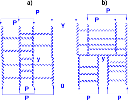
Therefore, we have to assume that . As we have discussed, generally speaking, it means that our problem has no solution. However, in QCD the situation is much better. Indeed, to generate a correct vertex we need to introduce . The Feymann diagrams for this transition are obvious (see Fig. (2-b). However, the main contribution stems from the diagrams of Fig. (2-a) - type which are of the order of . Therefore, diagrams of Fig. (2-b) - type are small corrections to the main contribution and could be negative, in spite of the fact that the diagrams shown in Fig. (2-b) actually give a positive contribution. We will discuss this scenario in all details in our paper [18].
6 Conclusions
Being elegant and beautiful the BFKL Pomeron Calculus has a clear disadvantage: it is not a theoretically closed theory. Indeed, we need to add to the formalism of the BFKL Pomeron Calculus the theoretical ideas what kind of Pomeron interactions we should take into account and why. Of course, the Feymann diagrams in leading log approximation of perturbative QCD allow us, in principle, to calculate all possible Pomeron interactions but, practically, it is a very hard job. Even if we will calculate these vertices we need to understand what set of vertices we should take into account for the calculation of the scattering amplitude. This is the reason why we need to develop a more general formalism. Fortunately, such a formalism has been built and it is known under the abbreviation JIMWLK-Balitsky approach [30, 27, 23]. In this approach we are able to calculate all vertices for Pomeron interactions as it was demonstrated in Ref. [31] and it solves the first part of the problem: determination of all possible Pomeron interactions. However, we need to understand what vertices we should take into account for the calculation of the scattering amplitude. We hope that a further progress in going beyond of the BFKL Pomeron Calculus (see Refs. [31, 32]) will lead to such a development of the BFKL Pomeron Calculus that we will have a consistent theoretical approach. Hopefully this approach will be simpler than Lipatov’s effective action [33] which is not easier to solve than the full QCD Lagrangian.
The probabilistic interpretation gives a practical method for creating a Monte Carlo code in spirit of the approach suggested in Ref. [34]. This code will allow us to find a numerical solution to the problem and to consider the inclusive observables. This extension is very desirable since most of the experimental data exist just for these observables.
This year my teacher, Prof. Gribov, would have been 75 years old. I am happy to report him that his ideas are still alive and still give the simplest and the most elegant approach to high energy interaction. The high energy behaviour of the scattering amplitude is still an open theoretical question. We have learned a lot and we are able to foresee a lot of difficulties ahead. Therefore, it is a good problem to be solved.
References
- [1] L. V. Gribov, E. M. Levin and M. G. Ryskin, Phys. Rep. 100, 1 (1983).
- [2] A. H. Mueller and J. Qiu, Nucl. Phys.,427 B 268 (1986) .
- [3] E. A. Kuraev, L. N. Lipatov, and F. S. Fadin, Sov. Phys. JETP 45, 199 (1977); Ya. Ya. Balitsky and L. N. Lipatov, Sov. J. Nucl. Phys. 28, 22 (1978).
- [4] J. Bartels, M. Braun and G. P. Vacca, Eur. Phys. J. C40, 419 (2005) [arXiv:hep-ph/0412218] ; J. Bartels and C. Ewerz, JHEP 9909, 026 (1999) [arXiv:hep-ph/9908454] ; J. Bartels and M. Wusthoff, Z. Phys. C66, 157 (1995) ; A. H. Mueller and B. Patel, Nucl. Phys. B425, 471 (1994) [arXiv:hep-ph/9403256]; J. Bartels, Z. Phys. C60, 471 (1993).
- [5] M. Braun, arXiv:hep-ph/0504002 ; Eur. Phys. J. C16, 337 (2000) [arXiv:hep-ph/0001268]; M. Braun, Eur. Phys. J. C6, 321 (1999) [arXiv:hep-ph/9706373]; M. A. Braun and G. P. Vacca, Eur. Phys. J. C6, 147 (1999) [arXiv:hep-ph/9711486].
- [6] H. Navelet and R. Peschanski, Nucl. Phys. B634, 291 (2002) [arXiv:hep-ph/0201285]; Phys. Rev. Lett. 82, 137 (1999), [arXiv:hep-ph/9809474]; Nucl. Phys. B507, 353 (1997) [arXiv:hep-ph/9703238].
- [7] J. Bartels, L. N. Lipatov and G. P. Vacca, Nucl. Phys. B706, 391 (2005) [arXiv:hep-ph/0404110].
- [8] V. N. Gribov, Sov. Phys. JETP 26, 414 (1968) [Zh. Eksp. Teor. Fiz. 53, 654 (1967)].
- [9] P. Grassberger and K. Sundermeyer, Phys. Lett. B77, 220 (1978).
- [10] E. Levin, Phys. Rev. D49, 4469 (1994).
- [11] K. G. Boreskov, “Probabilistic model of Reggeon field theory,” arXiv:hep-ph/0112325 and reference therein.
- [12] C.W. Gardiner,“Handbook of Stochastic Methods for Physics, Chemistry and the Natural Science”, Springer-Verlag, Berlin, Heidelberg 1985.
- [13] A. H. Mueller, Nucl. Phys. B415, 373 (1994); ibid B437, 107 (1995).
- [14] E. Levin and M. Lublinsky, Nucl. Phys. A730, 191 (2004) [arXiv:hep-ph/0308279].
- [15] E. Levin and M. Lublinsky, Phys. Lett. B607, 131 (2005) [arXiv:hep-ph/0411121].
- [16] E. Levin and M. Lublinsky, Nucl. Phys. A (in press), arXiv:hep-ph/0501173.
- [17] E. Levin, Nucl. Phys. A (in press), arXiv:hep-ph/0502243.
- [18] E. Levin and A. Prygarin , (in preparation).
- [19] E. Iancu and D. N. Triantafyllopoulos, Nucl. Phys. A756, 419 (2005) [arXiv:hep-ph/0411405]; Phys. Lett. B610, 253 (2005) [arXiv:hep-ph/0501193].
- [20] A. H. Mueller, A. I. Shoshi and S. M. H. Wong, Nucl. Phys. B715, 440 (2005) [arXiv:hep-ph/0501088].
- [21] L. N. Lipatov, Phys. Rept. 286, 131 (1997) [arXiv:hep-ph/9610276]; Sov. Phys. JETP 63, 904 (1986) and references therein.
- [22] E. Iancu, G. Soyez and D. N. Triantafyllopoulos, arXiv:hep-ph/0510094.
- [23] I. Balitsky, [arXiv:hep-ph/9509348]; Phys. Rev. D60, 014020 (1999) [arXiv:hep-ph/9812311].
- [24] Y. V. Kovchegov, Phys. Rev. D60, 034008 (1999), [arXiv:hep-ph/9901281].
- [25] H. Weigert, Prog. Part. Nucl. Phys. 55, 461 (2005), arXiv:hep-ph/0501087 and references therein.
- [26] J. P. Blaizot, E. Iancu and H. Weigert, Nucl. Phys. A713, 441 (2003), [arXiv:hep-ph/0206279].
- [27] J. Jalilian-Marian, A. Kovner, A. Leonidov and H. Weigert, Phys. Rev. D59, 014014 (1999), [arXiv:hep-ph/9706377]; Nucl. Phys. B504, 415 (1997), [arXiv:hep-ph/9701284]; J. Jalilian-Marian, A. Kovner and H. Weigert, Phys. Rev. D59, 014015 (1999), [arXiv:hep-ph/9709432]; A. Kovner, J. G. Milhano and H. Weigert, Phys. Rev. D62, 114005 (2000), [arXiv:hep-ph/0004014] ; E. Iancu, A. Leonidov and L. D. McLerran, Phys. Lett. B510, 133 (2001); [arXiv:hep-ph/0102009]; Nucl. Phys. A692, 583 (2001), [arXiv:hep-ph/0011241]; E. Ferreiro, E. Iancu, A. Leonidov and L. McLerran, Nucl. Phys. A703, 489 (2002), [arXiv:hep-ph/0109115]; H. Weigert, Nucl. Phys. A703, 823 (2002), [arXiv:hep-ph/0004044].
- [28] E. Iancu and A. H. Mueller, Nucl. Phys. A730 (2004) 460, 494, [arXiv:hep-ph/0308315],[arXiv:hep-ph/0309276].
- [29] M. Kozlov and E. Levin, Nucl. Phys. A739 (2004) 291 [arXiv:hep-ph/0401118].
- [30] L. McLerran and R. Venugopalan, Phys. Rev. D 49,2233, 3352 (1994); D 50,2225 (1994); D 53,458 (1996); D 59,09400 (1999).
- [31] A. Kovner and M. Lublinsky, ArXiv:hep-ph/0510047; arXiv:hep-ph/0503155; Phys. Rev. Lett. 94, 181603 (2005) [arXiv:hep-ph/0502119]; JHEP 0503, 001 (2005) [arXiv:hep-ph/0502071]; Phys. Rev. D71, 085004 (2005) [arXiv:hep-ph/0501198].
- [32] Y. Hatta, E. Iancu, L. McLerran and A. Stasto, arXiv:hep-ph/0505235; arXiv:hep-ph/0504182.
- [33] L. N. Lipatov, Nucl. Phys. B452, 69 (1995).
- [34] A. H. Mueller and G. P. Salam, Nucl. Phys. B475, 293 (1996), [arXiv:hep-ph/9605302]; G. P. Salam, Nucl. Phys. B461, 512 (1996).