The soft and the hard pomerons
in hadron elastic scattering at small $t$

Abstract

We consider simple-pole descriptions of soft elastic scattering for $pp$, $\bar{p}p$, $\pi^{\pm}p$ and $K^{\pm}p$. We work at $t$ and $s$ small enough for rescatterings to be neglected, and allow for the presence of a hard pomeron. After building and discussing an exhaustive dataset, we show that simple poles provide an excellent description of the data in the region $-0.5$ GeV${}^{2}\leq t\leq-0.1$ GeV², 6 GeV$\leq\sqrt{s}\leq$ 63 GeV. We show that new form factors have to be used, and get information on the trajectories of the soft and hard pomerons.

Keywords: Hadron elastic scattering
PACS: 13.85.-t,13.85.Dz, 11.55.-m, 12.40.Na, 13.60.Hb

Introduction

In recent papers [1], we have shown that a model which includes a hard pomeron reproduces very well the total cross sections and the ratios $\rho$ of the real to imaginary parts of the forward scattering amplitude, while the description obtained from a soft pomeron only is much less convincing [2]. We considered the full set of forward data [3] for $pp$, $\bar{p}p$, $Kp$, $\pi p$, $\gamma p$ and $\gamma\gamma$, and showed that the description extends down to $\sqrt{s}=5$ GeV.

However, if one uses a simple pole for the hard pomeron and a fit to all data for $\sqrt{s}\geq 5$ GeV, the coupling of this new trajectory is almost zero in $pp$ scattering, while it is non negligible in $Kp$ and $\pi p$. The reason is simple: a hard pole, with an intercept of about 1.45, needs to be unitarised at high energy. Hence the high-energy $\bar{p}p$ data almost decouple any fast-rising pole. To see the hard singularity, one thus needs to limit the energy range of the fit, and we found that for centre-of-mass energies 5 GeV$\leq\sqrt{s}\leq$ 100 GeV the data were well described by a sum of four simple poles: a charge-conjugation-odd ($C=-1$) exchange (corresponding to the $\rho$ and $\omega$ exchanges and denoted $R_{-}$) with intercept 0.47, and three $C=+1$ exchanges, with intercepts 0.61 ($f$ and $a_{2}$ trajectories denoted $R_{+}$), 1.073 (soft pomeron $S$) and 1.45 (hard pomeron $H$).

We then showed that it is possible to extend the fit to high energies, provided that one unitarises the hard pomeron. The low-energy description remains dominated by the pole term, whereas the multiple scatterings tame the growth at high energy. However, despite the fact that the hard pomeron intercept is very close to what is observed in deeply inelastic scattering [6] and in photoproduction [7], it is not entirely sure that it is present in soft scattering. Indeed, its couplings are small and its contribution is less than 10% for $\sqrt{s}<100$ GeV. Hence it is important to look for confirmation of its presence in other soft processes, and the obvious place to start from is elastic scattering.

Although elastic scattering has been studied for a long time, its description within Regge theory poses several problems:

• There is no standard dataset: the data are present in the HEPDATA system [8], but they have not been gathered into a common format, some of the included datasets are not published, and several are superseded. Furthermore, the treatment of systematic errors is often obscure. This may explain why many authors neglect the quality of their fits: most existing models do not reproduce the data in a statistically acceptable manner.

• Maybe because of the absence of a standard dataset, most theoretical works concentrate on $pp$ and $\bar{p}p$ data, and neglect $\pi p$ and $Kp$ elastic scattering. As we showed in [1], this may however be the place to look for a hard pomeron.

• On the theoretical side, the situation is also more difficult: whereas at $t=0$ one had to introduce coefficients in front of the Regge exchanges, one now has to use form factors. These are a priori unknown. Also, there is no reference fit with an acceptable $\chi^{2}$ per degree of freedom ($\chi^{2}$/d.o.f.).

• For the purpose of this paper, one has to implement several cutoffs: first of all, the energy has to be sufficient to use leading exchanges, and small enough to be able to neglect rescatterings (especially when we consider contributions from a hard pomeron). Similar cut-offs need to be implemented in the off-forward case: first of all, many datasets have inconsistencies in the first few bins, so that $|t|$ needs to be large enough. At the same time, one needs to be far from the dip region, where rescatterings are notoriously important. Thus there must also be an upper cutoff in $|t|$.

Our strategy in this paper will be to fix the parameters entering the description of the data at $t=0$ [1], and to compare a model containing only a soft pomeron with a model where we add a hard pomeron. After a theoretical summary fixing the conventions, we shall recall the parametrisation of forward data in section 2. In section 3, we will present the dataset which we are using, discuss the problem of systematic errors, and use a general method [9] to determine the functions describing the form factors of the various Regge exchanges. As an output, we shall also be able to determine the position of the first cone in $t$, i.e. the region where the rescatterings can be neglected. In section 4, we shall then produce a fit using only a soft pomeron, and show that it describes very well the elastic data. In section 5, we shall give our results for the hard pomeron case, and give constraints on its form factors and slope.

1 Theoretical framework

We shall parametrise all exchanges by simple poles, and limit ourselves to a region in $s$ and $t$ where these are dominant. The amplitude $A^{ab}(s,t)$ that describes the elastic scattering of hadrons $a$ and $b$ is normalised so that the total and the differential elastic cross sections are given by

$$\sigma_{tot}^{ab}(s) = \frac{1}{2q_{ab}\sqrt{s}}\Im mA^{ab}(s,0),$$ (1)

$$\frac{d\sigma_{el}^{ab}(s,t)}{dt} = \frac{1}{64\pi sq_{ab}^{2}}|A^{ab}(s,t)|^{2},$$ (2)

where $q_{ab}=\sqrt{[(s-m_{a}^{2}-m_{b}^{2})^{2}-4m_{a}^{2}m_{b}^{2}]/4s}$ is the momentum of particles $a$ and $b$ in the centre-of-mass system.

Regge theory implies that one can write $A(s,t)\equiv A(z_{t},t)$ where the Regge variable, $z_{t}$, is the cosine of the scattering angle in the crossed channel:

$$z_{t}=\frac{t+2s_{ab}}{\sqrt{(4m_{a}^{2}-t)(4m_{b}^{2}-t)}}$$ (3)

with $s_{ab}=s-m_{a}^{2}-m_{b}^{2}$.

A simple-pole singularity (reggeon) in the complex $j$ plane at $j=\alpha(t)$ then leads to a term in the amplitude given by

$$A_{R}^{ab}(z_{t},t)=16\pi^{2}[2\alpha(t)+1]\frac{\Gamma(\alpha(t)+1/2)}{\sqrt{\pi}\Gamma(\alpha(t)+1)}\beta^{a}(t)\beta^{b}(t)\eta(\alpha(t))P_{\alpha(t)}(z_{t}),$$ (4)

where $\alpha(t)$ is the trajectory of the reggeon, $\beta^{i}(t)$ is the coupling of the reggeon with particle $i$: $t$-channel unitarity implies that the couplings factorise, and that the dependence on the beam $a$ and target $b$ enters through the product $\beta^{a}(t)\beta^{b}(t)$. The signature factor $\eta(\alpha(t))$ can be written

$$\eta_{\xi}(\alpha(t))=\left\{\begin{array}[]{ll}\displaystyle-\frac{\exp(-i\pi\alpha(t)/2)}{\sin(\pi\alpha(0)/2))}&\quad({\rm crossing\ even},\ C=+1),\\ \displaystyle-i\frac{\exp(-i\pi\alpha(t)/2)}{\cos(\pi\alpha(0)/2))}&\quad({\rm crossing\ odd},\ C=-1).\end{array}\right.$$ (5)

At high energy $s\gg-t$, $z_{t}$ is large. This allows, taking into account the asymptotics of the Legendre polynomials and using the variable

$$\tilde{s}_{ab}=\frac{t+2s_{ab}}{s_{0}},\qquad\mbox{with}\quad s_{0}=1\ \mbox{GeV}^{2}$$ (6)

instead of $z_{t}$, to re-absorb many of the factors of Eq.(4) into the definition of the couplings so that, for the scattering of $a$ on protons, the simple-pole contribution to the amplitude becomes

$$A_{R}^{ap}(\tilde{s}_{ap},t)=\frac{g^{a}_{R}}{2^{\alpha_{R}(0)}}F^{a}_{R}(t)F^{p}_{R}(t)\ \eta_{\xi}({\alpha_{R}(t)})\ \tilde{s}_{ap}^{\alpha_{R}(t)}.$$ (7)

with $F^{a}_{R}(0)=1$, $a=$ $p$, $\pi$, $K$.

1.1 Trajectories

At high enough energies ($\sqrt{s}\geq 5$ GeV [1]), the amplitude is dominated by a few exchanged trajectories.

For the $C=-1$ part, we shall restrict ourselves to a region in $t$ where it is enough to consider meson trajectories: one of the reasons to limit ourselves to the first cone is that we can forget the odderon contribution, which is known to be negligible at $t=0$.

For the $C=+1$ part, we shall first consider meson exchanges, as well as a soft pomeron and a hard pomeron.

We shall consider here scattering of $p$, $\bar{p}$, $\pi^{\pm}$ and $K^{\pm}$ on protons, and we summarise the possible exchanged trajectories in Table 1.

$a$	$C=+1$	$C=-1$	$A^{ap}(s_{ap},t)$
$p$	$P,f,a_{2}$	$\omega,\rho$	$A^{pp}=P+f+a_{2}-\omega-\rho,$
$\bar{p}$			$A^{\bar{p}p}=P+f+a_{2}+\omega+\rho,$
$\pi^{+}$	$P,f$	$\rho$	$A^{\pi^{+}p}=P+f-\rho,$
$\pi^{-}$			$A^{\pi^{-}p}=P+f+\rho,$
$K^{+}$	$P,f,a_{2}$	$\omega,\rho$	$A^{K^{+}p}=P+f+a_{2}-\omega-\rho,$
$K^{-}$			$A^{K^{-}p}=P+f+a_{2}+\omega+\rho,$

Table 1: The trajectories entering the amplitudes considered in this paper.

Generally, the $\omega$, $\rho$, $f$ and $a_{2}$ trajectories are different: they do not have coinciding intercepts or slopes[10]. However, as each trajectory comes with three form factors, we shall have to assume degeneracy for the $C=+1$ and for the $C=-1$ trajectories [11], in order to limit the number of parameters.

Hence the model that we are considering can be written:

$$A^{ap}(s,t)=A_{+}^{ap}(\tilde{s}_{ap},t)+A_{S}^{ap}(\tilde{s}_{ap},t)+A_{H}^{ap}(\tilde{s}_{ap},t)\mp A^{ap}_{-}(\tilde{s}_{ap})$$ (8)

with the $-$ sign for the (positively charged) particles.

2 Description of the forward data

We have shown in [1] that the data for $pp$, $\bar{p}p$, $\pi^{\pm}p$, $K^{\pm}p$, $\gamma p$ and $\gamma\gamma$ can be well described from $\sqrt{s}=5$ GeV to 100 GeV by either a soft pomeron, or a mixture of a soft pomeron and a hard pomeron, the latter case being significantly better. We have also shown that the inclusion of the subtraction constants that enter the dispersion relations lead to a better description of the real part of the amplitude. The formula for the $\rho$ parameter is then given by

$$\rho_{\pm}\,\sigma_{\pm}=\frac{R_{ap}}{p}+\frac{E}{\pi p}{\textrm{P}}\int_{m_{a}}^{\infty}\left[\frac{\sigma_{\pm}}{E^{\prime}(E^{\prime}-E)}-\frac{\sigma_{\mp}}{E^{\prime}(E^{\prime}+E)}\right]p^{\prime}\,dE^{\prime}$$ (9)

where the $+$ sign refers to the process $ap\rightarrow ap$ and the $-$ sign to $\bar{a}p\rightarrow\bar{a}p$, $E$ and $p$ are the energy and the momentum of $a$ in the proton rest frame, P indicates a principal-part integral, $R_{ap}$ is the subtraction constant, and $\sigma$ are the total cross sections. They are given by Eqs. (1, 8) for $\sqrt{s}\geq 5$ GeV, and fitted directly to the data at lower energy [1].

We give in Table 2 the values of the parameters resulting for a fit to all data for $\sigma_{tot}$ and $\rho$ for $\bar{p}p$, $pp$, $\pi^{\pm}p$ and $K^{\pm}p$, and for $\sigma_{tot}$ for $\gamma p$ and $\gamma\gamma$. We quote the values obtained in [1] (for a model with both a soft and a hard pomeron), and follow the same procedure for a model with a soft pomeron only. Table 3 shows the quality of the fits. Clearly, even in this modest energy range, the inclusion of a hard pomeron makes the fits much better, particularly those to the $\rho$ parameter for pions and kaons. Converting the $\chi^{2}$/d.o.f. into a confidence level (CL), one gets for the overall soft pomeron CL=6%, whereas the fit including a hard pomeron achieves CL=93%. Nevertheless, as the existence of the hard pomeron is not totally settled, we shall keep both models in the following, and see how well they fare in the description of the elastic data.

Parameter	soft pomeron	soft & hard pomerons
$\alpha_{S}(0)$	1.0927	1.0728
$\alpha_{H}(0)$	-	1.45
$\alpha_{+}(0)$	0.61	0.61
$\alpha_{-}(0)$	0.47	0.47
$g_{H}^{p}$	-	0.10
$g_{H}^{\pi}$	-	0.28
$g_{H}^{K}$	-	0.30
$g_{S}^{p}$	49.5	56.2
$g_{S}^{\pi}$	31.4	32.7
$g_{S}^{K}$	27.7	28.3
$g_{+}^{p}$	177	158
$g_{+}^{\pi}$	78	78
$g_{+}^{K}$	43	46
$g_{-}^{p}$	81	79
$g_{-}^{\pi}$	13.9	14.2
$g_{-}^{K}$	32	32

Table 2: Values of the intercepts and couplings ($t=0$).

Quantity	Number	soft	soft and hard
	of points $N$	$\chi^{2}/N$	$\chi^{2}/N$
$\sigma_{tot}^{pp}$	104	1.2	0.86
$\sigma_{tot}^{\bar{p}p}$	59	0.78	0.88
$\sigma_{tot}^{\pi^{+}p}$	50	1.2	0.78
$\sigma_{tot}^{\pi^{-}p}$	95	0.90	0.90
$\sigma_{tot}^{K^{+}p}$	40	0.93	0.72
$\sigma_{tot}^{K^{-}p}$	63	0.72	0.62
$\sigma_{tot}^{\gamma p}$	38	0.61	0.57
$\sigma_{tot}^{\gamma\gamma}$	34	0.87	0.74
$\rho^{pp}$	64	1.59	1.62
$\rho^{\bar{p}p}$	9	0.49	0.43
$\rho^{\pi^{+}p}$	8	2.8	1.52
$\rho^{\pi^{-}p}$	30	1.8	1.09
$\rho^{K^{+}p}$	10	0.72	0.70
$\rho^{K^{-}p}$	8	1.7	0.90
Total	603	1.07	0.95

Table 3: Partial $\chi^{2}$ for the total cross sections $\sigma_{tot}$ and the ratios $\rho$.

3 The elastic dataset

Throughout the last 40 years, there have been many measurements of the differential elastic cross sections [12-71]. In the present paper, we shall use not only $pp$ and $\bar{p}p$ data, but also $K^{\pm}p$ and $\pi^{\pm}p$ data as the hard pomeron seems to couple more to mesons [1]. Fortunately, most of these measurements have been communicated to the HEPDATA group [8], so that one does not need to re-encode all the data. However, some basic work still needs to be done, as there are 80 papers, with different conventions, and various units. Once the translation into a common format has been achieved, there are still a number of issues to be dealt with:

• Some of the data are preliminary or redundant. We chose to include only final published data in the set that we are building;

• The main systematic error usually comes from a poor knowledge of the beam luminosity. This means that all the data of one run taken in a given experiment at a given energy can be shifted up or down by a certain amount. Although we shall mostly treat these errors as random (and add them quadratically to the statistical error), we have encoded this information in the dataset. Hence we have split the data into subsets, to which correspond data in a given paper with the same systematic error. This defines 263 different subsets of the data, shown in Appendix 1. We shall also use this information to exclude subsets which blatantly contradict the rest of the dataset.

• Several experiments have not spelled out their systematic errors in the published work, and these have to be reconstructed. Indeed, many measurements are not absolute, but rather normalised by extrapolating to the optical point $d\sigma_{el}/dt(t=0)$, which is known from measurements of the total cross section. In that case, we have assigned the error on the optical point (ı.e. twice that on the total cross section used) as a systematic error on the subset.

• In the case of bubble chamber experiments, such as [38], the luminosity was monitored, but it was included in the systematic uncertainty added to the statistical one. We have thus subtracted it so that these data can be shifted in the same way as the others.

• In the case of [71], we have added the $t$-dependent systematics to the statistical error, and allowed 4% in the global normalisation.

• As we shall see in the subsequent sections of this paper, some of the subsets [39, 34, 22, 14] are in strong disagreement with the other sets considered. We shall eventually exclude them from our analysis.

The global dataset [72] contains 10188 points (we have restricted it to data at $\sqrt{s}\geq 4$ GeV). We show some of its details in the tables of the Appendix. The present analysis, which concentrates on the first cone, will include about a fourth of these data, as explained in the next section, and shown in Table 4.

observable	$N_{pp}$	$N_{\bar{p}p}$	$N_{\pi^{+}p}$	$N_{\pi^{-}p}$	$N_{K^{+}p}$	$N_{K^{-}p}$	$N_{tot}$
$\sigma_{tot}$ (full set, all $\sqrt{s}$)	261	444	412	606	208	416	2347
this analysis	104	50	50	95	40	63	402
$\rho$ (full set, all $\sqrt{s}$)	116	90	9	39	22	15	291
this analysis	64	9	8	30	10	8	129
$d\sigma_{el}/dt$ (full set, $\sqrt{s}\geq 4$ GeV)	4639	1252	802	2169	595	731	10188
this analysis	818	281	290	483	166	169	2207
after exclusion	795	226	281	478	166	169	2115

Table 4: The statistics of the full dataset and of the present analysis.

The forward fit of section 1 gave us the intercepts and the couplings $g_{\pm}$, $g_{S}$ and $g_{H}$. To extend it to non-zero $t$, we need to find the form factors. These are a priori unknown, so that one has to deal with arbitrary functions.

3.1 Form factors and local fits

In order to obtain the possible form factors, we shall scan the dataset at fixed $t$, i.e. we shall fit a complex amplitude with constant form factors to the data in small bins of $t$ (and refer to these fits as $local$ fits). The constants that we get will then depend on $t$ and give us a picture of the form factor. The value of the $\chi^{2}$ will also tell us in which region of $t$ we should work.

This strategy however will not work for the general case considered here: each bin does not contain enough points to have a unique minimum. We can take advantage of the fact that both models considered here give the same values for the intercept of the crossing-odd Reggeon contribution, and for the crossing-even ones as well (see Table 2). We can also read off the slopes from a Chew-Frautschi plot. This gives the following $f/a_{2}$ and $\rho/\omega$ trajectories:

$$\alpha_{+} = 0.61+0.82~{}t,$$

$$\alpha_{-} = 0.47+0.91~{}t.$$ (10)

Furthermore, we shall not be able to include a hard pomeron in the local fits as its contribution is too small to be stable.

We fit all the data from 6 GeV$\leq\sqrt{s}\leq 63$ GeV, and we choose small bins of width 0.02 GeV². We restrict ourselves to independent bins where we have more than four points for each process.

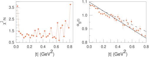
Figure 1: The results of the local fits for the $\chi^{2}$ per number of points (left) and for the pomeron trajectory (right). The dashed curve is from [73] and the plain curve results from the global fit given in the next section.

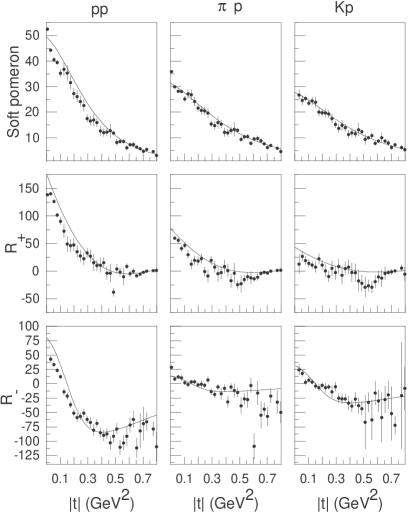
Figure 2: The results of the local fits for the residues of the poles. The curves are the results of a global fit explained in the next section.

Each of these fits gives us a values of the $\chi^{2}$ per number of points, the coefficients $g_{R}^{ap}F^{p}_{R}(t)F^{a}_{R}(t)$, as well as $\alpha_{S}(t)$ for each $t$. We show these results in Figs. 1 and 2. The $\chi^{2}$ curve of Fig. 1 shows two things: first of all, the fit is never perfect, and this can be traced back to incompatibilities in the data. We shall come back to this in the next section, when we perform a global fit to all data. The second lesson is that the simple-pole description of the data has a chance to succeed in a limited region: the $\chi^{2}$ grows fast both at low $|t|$ (partly because the Coulomb interaction begins to matter) and for $|t|>0.6$ (where multiple exchanges come into play). To be conservative, we shall consider in the following the region $0.1\leq|t|\leq 0.5$. The right-hand graph in Fig. 1 shows the soft pomeron trajectory. It is very linear as a function of $t$. Its intercept and slope are somewhat different from the standard ones [73].

Figure 2 shows the results for the residues of the poles $g^{a}F_{R}^{a}(t)F_{R}^{p}(t)$. In all cases, it is obvious that form factors must be different for different trajectories. There is in fact no reason why the hadrons should respond in the same way to different exchanges, as these have different quantum numbers and different ranges, and couple differently to quarks and gluons.

For the soft pomeron, we find that we can get a good description in the $pp$ and $\bar{p}p$ cases if we take

$$F^{p}_{S}(t)=\frac{1}{1-t/t_{S}^{(1)}+\left(t/t_{S}^{(2)}\right)^{2}}.$$ (11)

For $\pi$ and $K$ mesons, an adequate fit is provided by the monopole form factors

$$F^{a}_{S}(t)=\frac{1}{1-t/t^{a}_{S}},\qquad a=\pi,K.$$ (12)

The local fits for both the $C=+1$ and the $C=-1$ reggeons indicate that the form factors have a zero at some $t$ value. In the crossing-odd case, this is the well-known cross-over phenomenon [74]: the curves for $d\sigma/dt$ for $pa$ and $p\bar{a}$ cross each other at some value of $t$. In the crossing-even case, the zero is close to the upper value of $|t|$, so that we have evidence for a sharp decrease but not necessarily for a zero.

In each case, we have tried to obtain such zeroes through rescatterings. However, it is hard then to cancel both the real and the imaginary parts, and the zero moves with energy, or disappears when energy changes. We thus assume here, in a way which is consistent with the simple-pole hypothesis, that these zeroes are the same for $pp$, $\bar{p}p$, $\pi^{\pm}p$ and $K^{\pm}p$ scattering, and that they are fixed with energy: they can be thought of as a property of the form factors, or of the exchange itself, and are consistent with Regge factorisation.

We thus parametrise the $R_{-}$ and $R_{+}$ contributions as

$$A_{\pm}^{ap}(\tilde{s}_{ap},t)=Z^{a}_{\pm}(t)g^{a}_{\pm}F^{a}_{\pm}(t)F^{p}_{\pm}(t)\ \eta_{\xi}({\alpha_{\pm}(t)})\ \tilde{s}_{ap}^{\alpha_{\pm}(t)}.$$ (13)

For the form factors $F^{a}_{\pm}(t)$, we take the form

$$F^{p}_{\pm}(t)=\frac{1}{\left(1-t/t^{p}_{\pm}\right)^{2}}.$$ (14)

in the proton case, whereas we find that

$$F^{\pi,K}_{\pm}(t)=F_{S}^{\pi,K}(t)$$ (15)

gives us a good fit for $\pi$ and $K$.

The factor $Z^{a}_{\pm}(t)$ has a common zero $\zeta_{\pm}$, independent of $s$, for $p,\pi,K$, but a different one for the $C=+1$ and the $C=-1$ trajectories:

$$Z^{a}_{\pm}(t)=\frac{\tanh(1+t/\zeta_{\pm})}{\tanh(1)},\quad a=p,\pi,K.$$ (16)

We choose this simple form to restrict the growth of $Z^{a}_{\pm}$ with $t$.

Finally, when we shall introduce a hard pomeron, we shall find that a dipole form factor describes the proton data well

$$F^{p}_{H}(t)=\frac{1}{\left(1-t/t^{p}_{H}\right)^{2}},$$ (17)

whereas we can use the same form factor as for the soft pomeron to describe pions and kaons:

$$F^{\pi,K}_{H}(t)=F_{S}^{\pi,K}(t).$$ (18)

We summarise in Table 5 our choice of form factors. Of course, these are the simplest functions that reproduce the data at the values of $t$ considered here. Consideration of different $t$ ranges will probably call for more complicated parametrisations.

	$p$	$\pi$	$K$
$S$	$\displaystyle\frac{1}{1-t/t_{S}^{(1)}+(t/t_{S}^{(2)})^{2}}$	$\displaystyle\frac{1}{1-t/t^{\pi}}$	$\displaystyle\frac{1}{1-t/t^{K}}$
$C=+1$	$\displaystyle\frac{1}{(1-t/t_{+})^{2}}$	$\displaystyle\frac{1}{1-t/t^{\pi}}$	$\displaystyle\frac{1}{1-t/t^{K}}$
$C=-1$	$\displaystyle\frac{1}{(1-t/t_{-})^{2}}$	$\displaystyle\frac{1}{1-t/t^{\pi}}$	$\displaystyle\frac{1}{1-t/t^{K}}$
$H$	$\displaystyle\frac{1}{(1-t/t_{H})^{2}}$	$\displaystyle\frac{1}{1-t/t^{\pi}}$	$\displaystyle\frac{1}{1-t/t^{K}}$

Table 5: Parametrisation of the form factors.

4 Soft pomeron fit

Equipped with the information from the local fits, we can now perform a global fit to the elastic data for 0.1 GeV${}^{2}\leq|t|\leq$ 0.5 GeV², for 6 GeV$\leq\sqrt{s}\leq$ 63 GeV, and for a soft pomeron only. We fix the trajectories of the $C=+1$ and $C=-1$ exchanges according to Eq. (10).

The $\chi^{2}$/d.o.f. reaches the value 1.45, which is unacceptable for the number of points fitted (2207). Such a high value of the $\chi^{2}$ is largely due to contradictions between sets of data.

Parameter	soft pomeron	soft and hard pomerons
$\alpha\,^{\prime}_{S}$ (GeV-2)	0.332 $\pm$ 0.007	0.297 $\pm$ 0.010
$\alpha\,^{\prime}_{H}$ (GeV-2)	-	0.10 $\pm$ 0.21
$\alpha\,^{\prime}_{+}$ (GeV-2)	0.82 (fixed)	0.82 (fixed)
$\alpha\,^{\prime}_{-}$ (GeV-2)	0.91 (fixed)	0.91 (fixed)
$t_{S}^{(1)}$ (GeV2)	0.56 $\pm$ 0.01	0.56 $\pm$ 0.02
$t_{S}^{(2)}$ (GeV2)	2.33 $\pm$ 0.34	1.16 $\pm$ 0.06
$t_{H}$ (GeV2)	-	0.20 $\pm$ 0.05
$t_{+}$ (GeV2)	2.96 $\pm$ 0.25	2.34 $\pm$ 0.22
$t_{-}$ (GeV2)	7.97 $\pm$ 1.41	9.0 $\pm$ 1.8
$t^{\pi}$ (GeV2)	2.53 $\pm$ 0.14	2.89 $\pm$ 0.23
$t^{K}$ (GeV2)	3.92 $\pm$ 0.28	6.33 $\pm$ 0.94
$\zeta_{-}$ (GeV2)	0.148 $\pm$ 0.003	0.153 $\pm$ 0.003
$\zeta_{+}$ (GeV2)	0.47 $\pm$ 0.02	0.47 $\pm$ 0.03

Table 6: Values of the parameters (fit at $t\neq 0$).

We thus excluded the following data, which all have a CL less than $10^{-8}$: Bruneton [39] (sets 1050, 1204 and 1313, 25 points), Armitage [22] (set 1038, 12 points), Akerlof [14] $\bar{p}p$ for $\sqrt{s}=9.78$ GeV (set 1101, 20 points) and Bogolyubsky [34] (set 1114, 35 points). The removal of these 92 points (less than 5% of the data) brings the $\chi^{2}$/d.o.f. to 1.03, i.e. a confidence level of 20%.

The parameters of the fit are given in Table 6, and the partial $\chi^{2}$ in Table 7. We also show the form factors resulting from the global fit in Fig. 2. We see that there is good agreement with the local fits.

The main result is that the slope of the soft pomeron is higher than usually believed: $\alpha^{\prime}_{S}\approx 0.3$ GeV^-2. Also, the fit to near-forward data is remarkably good.

We also show in Figs. 3, 4, 5 and 6 some of the fits to the data. We see in Fig. 4 that our description extends very well to S$p\bar{p}$S energies. Also, the top-left of Fig. 4 shows the kind of disagreement that we had to remove: the points of Akerlof are in definite disagreement with those of Ayres. Similar graphs can be plotted for all the data that we removed. Furthermore, one can see e.g. in the data of Brick [38] in Fig. 6 that the first few points are in strong disagreement with other sets. Such problems explain the rather high value of $|t|_{min}$ that we had to use.

Finally, let us mention that we also considered a fit where one allows the data of one given set at one given energy to be shifted by a common factor within one systematic error while treating the statistical error through the usual $\chi^{2}$ minimisation. Such a procedure leads to a higher $\chi^{2}$/d.o.f., of the order of 1.15 [7], without affecting the parameters significantly. As the datasets do not have compatible slopes within the statistical errors, we preferred to present here the results based on errors added quadratically.

Quantity	Number	$\chi^{2}/N$	$\chi^{2}/N$
	of points	(soft)	(soft+hard)
$d\sigma^{pp}/dt$	795	0.90	0.86
$d\sigma^{\bar{p}p}/dt$	226	1.01	0.99
$d\sigma^{\pi^{+}p}/dt$	281	0.90	0.89
$d\sigma^{\pi^{-}p}/dt$	478	1.18	1.18
$d\sigma^{K^{+}p}/dt$	166	1.02	1.11
$d\sigma^{K^{-}p}/dt$	169	1.18	1.12
Total	2115	1.022	0.997

Table 7: Partial values of $\chi^{2}$, differential cross sections.

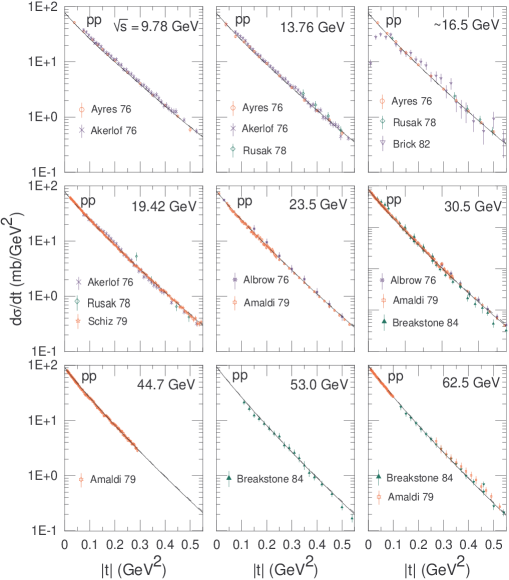
Figure 3: $pp$ differential cross sections. The plain curve shows the soft pomeron fit, and the dashed one the fit that includes a hard pomeron.

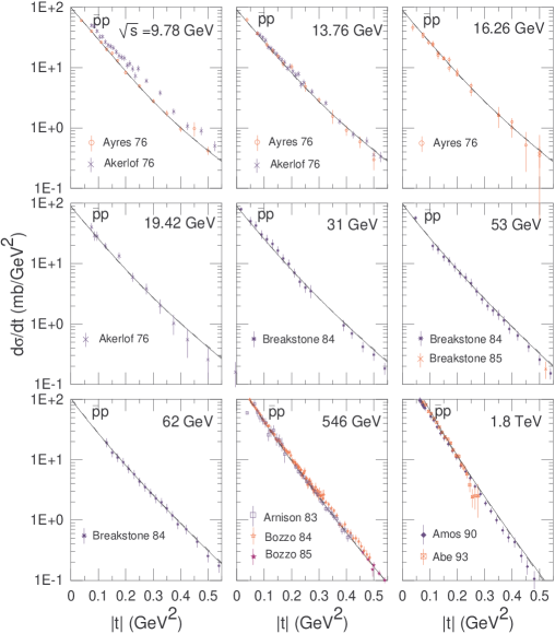
Figure 4: $p\bar{p}$ differential cross sections. The plain curve shows the soft pomeron fit, and the dashed one the fit that includes a hard pomeron.

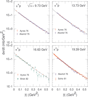
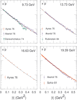
Figure 5: $\pi^{+}p$ and $\pi^{-}p$ differential cross sections.

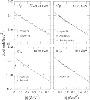
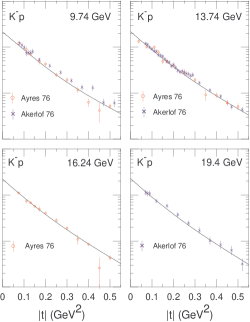
Figure 6: $K^{+}p$ and $K^{-}p$ differential cross sections.

5 Hard pomeron

One of the motivations of this paper was to confirm the presence of a small hard component in soft cross sections. The problem however is that the fit with only one soft pomeron is so good that a hard component is really not needed here. Following the philosophy of the previous section, we can nevertheless investigate the effect of its contribution in elastic data by fixing the parameters from the $t=0$ fit of Table 2 and constrain the form factors and trajectories. As can be seen from Table 7, the introduction of a hard pomeron makes the fit slightly better (the CL rises to about 48%) if we allow a different form factor from that of the soft pomeron in the $pp$ and $\bar{p}p$ cases. We obtain the parameters of the third column of Table 6. The hard pomeron slope is confirmed to be of the order of 0.1 GeV^-1, although the errors are large. We show in Fig. 7 the form factors of the various trajectories in this case. Note in the $pp$ and $\bar{p}p$ cases that the hard contribution is suppressed at higher $t$ by the form factor. Forcing it to be identical to the form factor of the soft pomeron results in a trajectory with a very large slope $\alpha^{\prime}_{H}\approx 1GeV^{-2}$.

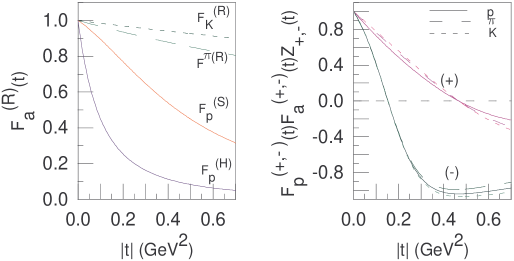
Figure 7: Form factors as function of $|t|$, in the model that includes a hard pomeron.

6 Conclusion

This paper has presented a few advances in the study of elastic cross sections:

• We have elaborated a complete dataset, including an evaluation of the systematic errors for all data. We have shown that statistical and systematic errors should be added in quadrature (i.e. the slopes of the data from different subsets are not consistent if one uses only statistical errors).

• We have shown that rescattering effects can be neglected in the region 0.1 GeV${}^{2}\leq|t|\leq 0.5$ GeV², 6 GeV$\leq\sqrt{s}\leq$ 63 GeV. This of course does not necessarily mean that the pomeron cuts are small, but rather that they can be re-absorbed in a simple-pole parametrisation [73].

• We showed that different trajectories must have different form factors. We confirm that the crossing-odd meson exchange has a zero. We also found evidence for a sharp suppression of the crossing-even form factor around $|t|=0.5$ GeV².

• The soft pomeron has a remarkably linear trajectory, and leads to a very good fit that extends well to S$p\bar{p}$S energies.

• Because of the quality of the soft pomeron fit, the elastic data do not confirm strongly the need for a hard pomeron. It is remarkable however that the hard pomeron fit gives 0.1 GeV^-2 for the central value of the slope, in agreement with [7].

It is our hope that this dataset, and this study, will serve as a starting point for precise studies of the whole range of elastic scattering, and especially for studies of unitarisation effects at higher $s$ or higher $t$, and for the comparison of several models.

Appendix: experimental data

$pp\rightarrow pp$

set	ref.	$\sqrt{s}$	$|t|_{min}$	$|t|_{max}$	syst.	number
		(GeV)	(GeV2)	(GeV2)		of points
1001	[14]	9.8 13.8 19.4	0.075	1.03 2.8 3.3	7%	50 61 55
1002	[15]	23.4 26.9 30.6	0.15 0.15 0.25	1.1 0.55 0.95	15%	19 8 15
		32.4 35.2 38.3	0.20 0.20 0.20	0.35 0.75 0.7		4 9 9
1014	[16]	4.5 4.9 5.3	0.14 0.10 0.27	2.1 2.7 3.5	15%	24 25 22
1015		6.2 6.4	0.058 0.070	6.0 1.9	8%	37 17
1037		4.6 4.8 5.0	2.0 2.2 2.5	8.6 9.6 10.5	7%	18 15 15
		5.3 5.8 6.2	7.6 9.1 9.7	13 15 17		4 9 4
		6.5	11	18		4
1039		6.8	0.083	6.7	10%	35
1020	[17]	23.5 30.7	0.042 0.016	0.24 0.11	1.2%	50 48
1021		30.7 44.7	0.11 0.05	0.46 0.29	2%	58 95
1030		23.5	0.25	0.79	3%	28
1022		23.5 30.7	0.83 0.90	3.0 5.8	5%	34 55
		44.7 62.5	0.62 0.27	7.3 6.3		65 74
1023		23.5	3.1	5.8	10%	21
1024		30.7	0.0011	0.008	0.40%	9
1025		62.5	0.0017	0.009	0.25%	16
1026		30.7	0.46	0.86	3.5%	11
1027		44.7	0.001	0.009	0.2%	24
1028		44.7 62.5	0.0092 0.0095	0.052 0.099	1%	46 49
1003	[18]	52.8	0.011	0.048	0.4%	36
1009	[19]	23.5 30.6	0.0004 0.0005	0.010 0.018	1%	31 32
		52.8 62.3	0.0011 0.0054	0.055 0.051		34 22
1004	[21]	9.0 10.0	0.0019	0.043 0.05	1.1%	20 18
1038	[22]	53.0	0.13	0.46	5%	12
1052	[23]	9.8	0.825	3.8	15%	17
1005	[25]	9.8 11.5 13.8	0.038	0.75 0.70 0.75	3%	16 17 18
		16.3 18.2	0.0375 0.075	0.80 0.75		19 15
1006	[32]	4.4 5.1 5.6	0.0008 0.0092 0.0089	0.013 0.10 0.11	2%	34 22 27
		6.1 6.2 6.5	0.0009 0.0011 0.015	0.11 0.014 0.11		67 35 30
		6.9 7.3 9.8	0.011 0.0093 0.0010	0.11 0.11 0.12		26 33 66
		7.7 8.0 8.3	0.011 0.0171 0.0093	0.11 0.11 0.11		29 24 28
		8.6 8.7 8.8	0.0009 0.0011 0.0009	0.11 0.015 0.11		65 47 65
		9.3 10.0 10.2	0.0114 0.0109 0.0108	0.12		29 34 29
		10.3 10.4 10.6	0.0008 0.013 .0008	0.015 0.12 0.015		37 35 44
		10.7 11.0 11.2	0.0108 0.013 0.011	0.12 0.12 0.12		33 33 30
		11.5	0.011 0.0010	0.12 0.11		26 156
1013	[36]	4.6	0.023	1.5	2%	97
1031	[37]	31.0 53.0 62.0	0.050 0.11 0.13	0.85	10%	24 24 23
1064		53.0	0.62	3.4	20%	31
1055	[38]	16.7	0.01	0.62	2%	26
1007	[40]	13.8 16.8	0.0022	0.039	1%	73 68
		21.7 23.8				64 60
1054	[43]	13.8 19.4	0.035	0.095	0.8%	7 7
1058	[44]	19.5 27.4	5.0 2.3	12 16	20%	31 87
1017	[46]	4.7	0.0028	0.14	1.6%${}^{\ref{opt}}$	13
1053	[48]	9.8	0.012	0.12	3%${}^{\ref{opt}}$	10
1042	[49]	5.0	0.011	0.34	15%	5
1044		5.6	0.019	0.56	13%	5
1045		6.1 7.1	0.036 0.064	0.79 1.0	20%	5 4
1046		6.5	0.032	1.1	17%	5
1019	[53]	4.5 5.5	0.016 0.027	5.1 4.9	15%	31 32
		6.3 7.6	0.032 0.079	3.8 2.8		30 29
1029	[54]	53.0	0.64	2.05	10%	15
1057	[55]	19.5 27.4	5.0 5.5	12 14	15%	34 30
1056	[56]	19.4	0.61	3.9	15%	33
1016	[57]	4.7 5.1 5.4	0.058 0.049 0.066	0.82 0.86 0.78	5%	13 13 12
		5.8 6.2	0.042 0.12	0.70 0.81		12 11
1018		4.7 5.5 6.2	0.2 0.22 0.23	0.89 0.74 0.79	5%	9 7 7
		6.5 6.9	0.24 0.25	0.81 0.75		7 6
1048	[58]	7.6 9.8 11.5	0.0027 0.0026 0.0028	0.119 0.12 0.12	2%${}^{\ref{opt}}$	21 23 21
1049	[59]	8.2 10.2 11.1	0.29 0.34 0.34	1.93 1.98 1.98	15%	21 20 20
		12.3 13.8 15.7	0.35	0.70 2.0 0.99		8 19 11
		16.8 17.9 18.9	0.35 0.35 0.29	2.1		32 29 30
		19.9 20.8 21.7	0.29	2.1 2.0 2.0		29 19 17
1043	[60]	5.0 6.0	0.13 0.19	2.0 3.6	7%	22 20
1040	[62]	4.5	0.0018	0.097	1%	55
1050	[39]	9.2	0.16	2.0	2%${}^{\ref{opt}}$	27
1036	[63]	10.0	0.0006	0.031	0.9%	72
1035		12.3	0.0007	0.029	0.69%	58
1034		19.4	0.0007	0.032	0.56%	69
1033		22.2	0.0005	0.030	0.57%	63
1032		23.9	0.0007	0.032	0.5%	66
1008		27.4	0.0005	0.026	0.52%	60
1010	[66]	52.8	0.83	9.8	5%	63
1041	[67]	4.9	1.2	2.5	10%	5
1011	[69]	13.8 19.4	0.55 0.95	2.5 10.3	15%	20 35
1012	[71]	19.4	0.021	0.66	4%	134

$\bar{p}p\rightarrow\bar{p}p$

set	ref.	$\sqrt{s}$	$|t|_{min}$	$|t|_{max}$	syst.	number
		(GeV)	(GeV2)	(GeV2)		of points
1130	[12]	546.0	0.026	0.078	0.52%	14
1132		1800.0	0.035	0.285	0.48%${}^{\ref{abe}}$	26
1101	[14]	9.8 13.8 19.4	0.075	1.0 0.95 0.75	7%	31 30 13
1102	[18]	52.8	0.011	0.048	1.54 %${}^{\ref{lum}}$	48
1103	[19]	30.4 52.6	0.0007 0.001	0.016 0.039	2.5%	29 28
		62.3	0.0063	0.038		17
1104		1800.0	0.034	0.63	9%	17 51
1105	[20]	6.9 7.0 8.8	0.19 0.83 0.075	0.58 3.8 0.58	5%	22 17 33
1106	[24]	540.0	0.045	0.43	8%	36
1107	[23]	7.6 9.8	0.53 0.83	5.4 3.8	15%	30 17
1108	[25]	9.8 11.5 13.8	0.038	0.75 0.5 0.75	3%	17 13 15
		16.3 18.2	0.075 0.038	0.6		11 13
1109	[29]	6.6	0.055	0.88	2.1 %${}^{\ref{opt}}$	43
1110	[30]	4.6	0.19	3.0	5%	35
1111	[31]	546.0	0.0022	0.035	2.5%	66
1112		630.0	0.73	2.1	15%	19
1126	[33]	5.6	0.11	1.3	10%	23
1114	[34]	7.9	0.055	1.0	0.8%${}^{\ref{opt}}$	52
1113	[35]	546.0	0.032	0.50	5%	87
1117		546.0	0.46	1.5	10%	34
1118	[36]	4.6	0.023	1.5	2%	97
1115	[37]	53.0	0.52	3.5	30%	27
1116		31.0 53.0 62.0	0.05 0.11 0.13	0.85	15%	22 24 23
1128	[43]	13.8 19.4	0.035	0.095	0.8%	7 7
1129	[54]	53.0	0.64	1.9	10%	8
1124	[57]	4.5 4.9	0.03 0.043	0.18 0.52	5%	6 10
1125		4.9 5.6	0.20 0.22	0.49 0.45	5%	5 4
1123	[62]	4.5	0.0018	0.097	1%	55
1127	[39]	8.7	0.17	1.24	2%${}^{\ref{opt}}$	11
1119	[64]	7.9	0.07	0.62	2%${}^{\ref{opt}}$	23
1131	[68]	4.5	0.76	5.5	5%	10
1121	[70]	5.6	0.085	1.2	5%	34
1120	[69]	13.8	0.55	2.5	15%	15
1122		19.4	0.95	3.8	35%	7

$\pi^{+}p\rightarrow\pi^{+}p$

set	ref.	$\sqrt{s}$	$|t|_{min}$	$|t|_{max}$	syst.	number
		(GeV)	(GeV2)	(GeV2)		of points
1212	[13]	21.7	0.08	0.94	2%${}^{\ref{opt}}$	18
1205	[14]	9.7 13.7 19.4	0.075	1.7 1.7 1.8	7%	70 63 53
1203	[21]	9.0 9.9	0.002 0.0019	0.043 0.05	1.1%	20 18
1214	[26]	7.8	0.075	0.68	1.4%${}^{\ref{opt}}$	13
1206	[23]	9.7	0.75	3.9	15%	22
1207	[25]	9.7 11.5	0.038	0.8 0.7	3%	19 17
		13.7 16.2 18.1	0.11 0.038 0.075	0.8		17 19 18
1215	[27]	4.4	0.46	17.3	15%	84
1201	[36]	4.5	0.023	1.5	2%	97
1210	[38]	16.6	0.01	0.58	2%${}^{\ref{brick}}$	25
1209	[43]	13.7 19.4	0.035	0.095	0.8%	7 7
1204	[39]	9.2	0.16	1.92	2%${}^{\ref{opt}}$	18
1202	[69]	5.2	0.65	3.8	10%	24
1208		13.7 19.4	0.55 0.95	2.5 3.4	15%	20 20
1211	[71]	19.4	0.022	0.66	4%${}^{\ref{sch}}$	133

$\pi^{-}p\rightarrow\pi^{-}p$

set	ref.	$\sqrt{s}$	$|t|_{min}$	$|t|_{max}$	syst.	number
		(GeV)	(GeV2)	(GeV2)		of points
1302	[14]	9.7 13.7 19.4	0.075	1.60 1.83 2.38	7%	64 60 61
1310		6.9 8.7	0.075	0.78 0.70	5%	38 38
1324		8.7	0.19	1.3	10%	28
1301	[21]	8.7	0.002	0.008	1.5%	21
1312		8.0 8.4 8.7	0.0012 0.0015 0.0016	0.025 0.03 0.034	1.5%	19 19 36
		9.3 9.8	0.0022 0.0028	0.05 0.056		17 18
		10.4 10.6	0.0035 0.0014	0.077 0.085		18 19
1314		8.7 9.7	0.0016 0.0022	0.021 0.035	1%${}^{\ref{opt}}$	20 34
1309	[23]	6.2 9.7	0.65 0.73	6.0 7.8	15%	22 46
1315	[25]	9.7 11.5	0.038	0.75 0.50	3%	18 13
		13.7 16.2 18.1	0.038	0.80 0.75 0.80		19 18 19
1304	[27]	6.2 7.6	7.4 10.	17 25	15%	6 4
1305	[36]	4.5	0.023	1.5	2%	97
1318	[40]	13.7 16.8 19.4	0.0022 0.0022 0.0023	0.039	1%	73 68 64
		21.7 23.7 24.7	0.0022			116 59 56
		25.5		0.038		57
1317	[42]	13.7	0.028	0.092	10%	5
1303	[43]	13.7 19.4	0.035	0.095	0.8%	7 7
1308	[45]	5.2	0.75	4.5	9%	25
1325		6.6	0.3	5.2	12%	44
1311	[50]	7.9 8.2 8.9	0.057 0.16 0.066	0.20 0.49 0.37	5%	14 18 25
		9.3 9.6 9.8	0.068 0.04 0.082	0.42 0.37 0.55		18 25 27
		10.2 10.2	0.054 0.055	0.53 0.46		19 17
1306		9.7	0.035	0.40	2.5%	37
1326	[52]	5.2	0.015	0.77	6%	41
1307	[60]	4.1 4.9 6.0	0.05 0.09 0.19	1.1 2.0 3.6	7%	23 24 20
1320	[61]	4.02 4.06 4.11	4.5	9.3 9.9 9.9	3%	25 28 28
		4.14 4.18 4.21	4.9	9.9 10.1 10.9		26 27 30
		4.26 4.30 4.33	5.3	10.7 10.5 10.7		26 22 21
1313	[39]	8.6	0.17	2.1	2%${}^{\ref{opt}}$	20
1321	[67]	4.8	1.2	2.4	10%	4
1322	[70]	5.6	0.15	1.8	5%	38
1316	[69]	13.7 19.4	0.55 0.95	2.5 10	15%	20 31
1319	[71]	19.4	0.021	0.66	4%	134

$K^{-}p\rightarrow K^{-}p$

set	ref.	$\sqrt{s}$	$|t|_{min}$	$|t|_{max}$	syst.	number
		(GeV)	(GeV2)	(GeV2)		of points
1414	[13]	21.7	0.12	0.94	2%${}^{\ref{opt}}$	17
1406	[14]	9.7 13.7 19.4	0.075 0.075 0.07	1.5 1.9 1.9	7%	21 35 35
1404	[21]	9.0 10.0	0.0019	0.043 0.050	1.1%	20 18
1408	[23]	9.7	0.75	7.0	15%	23
1407	[25]	9.7 11.5	0.038	0.70 0.65	3%	16 16
		13.7 16.2 18.2	0.075 0.075 0.038	0.75 0.70 0.75		13 16 17
1415	[28]	11.5	0.090	0.98	2.6%	36
1411	[38]	16.6	0.02	0.56	2%${}^{\ref{brick}}$	10
1402	[36]	4.5 5.2	0.023	1.5	2%	97 97
1409	[43]	13.7	0.045	0.095	0.8%${}^{\ref{opt}}$	6
1405	[39]	9.2	0.16	1.25	2%${}^{\ref{opt}}$	13
1401	[64]	7.8	0.09	1.4	2%${}^{\ref{opt}}$	48
1410	[69]	13.7 19.4	0.55 0.95	2.1 2.4	15%	16 12
1403		5.2	0.75	2.2	10%	12

$K^{-}p\rightarrow K^{-}p$

set	ref.	$\sqrt{s}$	$|t|_{min}$	$|t|_{max}$	syst.	number
		(GeV)	(GeV2)	(GeV2)		of points
1508	[20]	7.0 8.7	0.075	0.78	5%	38 38
1513		8.7	0.19	1.3	10%	28
1507	[23]	6.2	0.65	4.25	15%	16
1511	[25]	9.7 11.5 13.7	0.075 0.0375 0.0375	0.75 0.45 0.75	3%	14 12 16
		16.2 18.2	0.075	0.6 0.75		13 15
1510	[14]	9.7 13.7 19.4	0.070	1.4 1.7 1.0	7%	26 42 17
1501	[30]	4.5	0.19	2.3	5%	49
1503	[36]	4.5 5.2	0.023	1.5	2%	97 97
1502	[41]	4.5	0.0070	2.1	1.8%${}^{\ref{opt}}$	42
1505	[47]	5.3	0.010	2.4	2%${}^{\ref{opt}}$	27
1506	[51]	5.3	0.045	1.9	2%${}^{\ref{opt}}$	62
1509	[39]	8.6	0.17	2.0	2%${}^{\ref{opt}}$	13
1504	[65]	5.3	0.035	1.3	3%	41
1512	[69]	13.7 19.4	0.55 0.95	2.5 2.2	15%	20 8

References

- [1] J. R. Cudell, E. Martynov, O. Selyugin and A. Lengyel, Phys. Lett. B 587, 78 (2004) [arXiv:hep-ph/0310198]; J. R. Cudell, A. Lengyel, E. Martynov and O. V. Selyugin, Nucl. Phys. A 755, 587 (2005) [arXiv:hep-ph/0501288]; arXiv:hep-ph/0408332; in 11th International Conference on Quantum Chromodynamics (QCD 04), Montpellier, France, 2004 (to be published).
- [2] J. R. Cudell et al., Phys. Rev. D 65, 074024 (2002) [arXiv:hep-ph/0107219].
- [3] Review of Particle Physics, S. Eidelman et al., Phys. Lett. B 592, 1 (2004). Encoded data files are available at http://pdg.lbl.gov/2005/hadronic-xsections/hadron.html.
- [4] A. Donnachie and P. V. Landshoff, Phys. Lett. B 595, 393 (2004) [arXiv:hep-ph/0402081].
- [5] J. R. Cudell, V. Ezhela, K. Kang, S. Lugovsky and N. Tkachenko, Phys. Rev. D 61, 034019 (2000) [Erratum-ibid. D 63, 059901 (2001)] [arXiv:hep-ph/9908218].
- [6] A. Donnachie and P. V. Landshoff, Phys. Lett. B 518, 63 (2001) [arXiv:hep-ph/0105088]; ibid. 437, 408 (1998) [arXiv:hep-ph/9806344].
- [7] A. Donnachie and P. V. Landshoff, Phys. Lett. B 478, 146 (2000) [arXiv:hep-ph/9912312].
- [8] Durham Database Group (UK), M.R. Whalley et al., http://durpdg.dur.ac.uk/hepdata/reac.html.
- [9] L. A. Fajardo et al., Phys. Rev. D 24, 46 (1981); J. Kontros and A. Lengyel, in the proceedings of the 10th International Workshop on Soft Physics: Strong Interaction at Large Distances (Hadrons 94), Uzhgorod, Ukraine, 7-11 Sept. 1994, p. 104, edited by G.Bugrij, L.Jenkovszky and E.Martynov, (Bogolyubov Institute for Theoretical Physics, Kiev: 1994); P. Desgrolard, J. Kontros, A. I. Lengyel and E. S. Martynov, Nuovo Cim. A 110, 615 (1997) [arXiv:hep-ph/9707258].
- [10] P. Desgrolard, M. Giffon, E. Martynov and E. Predazzi, Eur. Phys. J. C 18, 555 (2001) [arXiv:hep-ph/0006244].
- [11] J. R. Cudell, K. Kang and S. K. Kim, Phys. Lett. B 395, 311 (1997) [arXiv:hep-ph/9601336].
- [12] F. Abe et al., Phys. Rev. D 50, 5518 (1994).
- [13] M. Adamus et al., Phys. Lett. B 186, 223 (1987), Yad. Fiz. 47, 722 (1988) [Sov. J. Nucl. Phys. 47, 722 (1988)].
- [14] C. W. Akerlof et al., Phys. Rev. D 14, 2864 (1976).
- [15] M. G. Albrow et al., Nucl. Phys. B 108, 1 (1976), ibid. 23, 445 (1970).
- [16] J. V. Allaby et al., Nucl. Phys. B 52, 316 (1973), Phys. Lett. B 28, 67 (1968), ibid. 27, 9 (1968).
- [17] U. Amaldi and K. R. Schubert, Nucl. Phys. B 166, 301 (1980).
- [18] M. Ambrosio et al., Phys. Lett. B 115, 495 (1982).
- [19] N. Amos et al., Nucl. Phys. B 262, 689 (1985), Phys. Lett. B 247, 127 (1990).
- [20] Y. M. Antipov et al., Yad. Fiz. 48, 138 (1988) [Sov. J. Nucl. Phys. 48, 85 (1988)]. Nucl. Phys. B 57, 333 (1973).
- [21] V. D. Apokin et al., Yad. Fiz. 25, 94 (1977), Nucl. Phys. B 106, 413 (1976), Yad. Fiz. 28, 1529 (1978) [Sov. J. Nucl. Phys. 28, 786 (1978)]. Yad. Fiz. 21, 1240 (1975) [Sov. J. Nucl. Phys. 21, 640 (1975)].
- [22] J. C. M. Armitage et al., Nucl. Phys. B 132, 365 (1978).
- [23] Z. Asad et al., Nucl. Phys. B 255, 273 (1985),
- [24] G. Arnison et al., Phys. Lett. B 128, 336 (1983).
- [25] D. S. Ayres et al., Phys. Rev. D 15, 3105 (1977).
- [26] I. V. Azhinenko et al., Yad. Fiz. 31, 648 (1980) [Sov. J. Nucl. Phys. 31, 337 (1980)].
- [27] C. Baglin et al., Nucl. Phys. B 216, 1 (1983), ibid. 98, 365 (1975).
- [28] M. Barth et al., Z. Phys. C 16, 111 (1982).
- [29] B. V. Batyunya et al., Yad. Fiz. 44, 1489 (1986) [Sov. J. Nucl. Phys. 44, 969 (1986)].
- [30] A. Berglund et al., Nucl. Phys. B 176, 346 (1980).
- [31] D. Bernard et al., Phys. Lett. B 198, 583 (1987), ibid. 171, 142 (1986).
- [32] G. G. Beznogikh et al., Nucl. Phys. B 54, 78 (1973).
- [33] D. Birnbaum et al., Phys. Rev. Lett. 23, 663 (1969).
- [34] M. Y. Bogolyubsky et al., Yad. Fiz. 41, 1210 (1985) [Sov. J. Nucl. Phys. 41, 773 (1985)].
- [35] M. Bozzo et al., Phys. Lett. B 155, 197 (1985), ibid. 147, 385 (1984).
- [36] G. W. Brandenburg et al., Phys. Lett. B 58, 367 (1975).
- [37] A. Breakstone et al., Nucl. Phys. B 248, 253 (1984), Phys. Rev. Lett. 54, 2180 (1985).
- [38] D. Brick et al., Phys. Rev. D 25, 2794 (1982).
- [39] C. Bruneton et al., Nucl. Phys. B 124, 391 (1977);
- [40] J. P. Burq et al., Nucl. Phys. B 217, 285 (1983);
- [41] J. R. Campbell et al., Nucl. Phys. B 64, 1 (1973);
- [42] T. J. Chapin et al., Phys. Rev. D 31, 17 (1985).
- [43] R. L. Cool et al., Phys. Rev. D 24, 2821 (1981).
- [44] S. Conetti et al., Phys. Rev. Lett. 41, 924 (1978).
- [45] P. Cornillon et al., Phys. Rev. Lett. 30, 403 (1973).
- [46] N. Dalkhazav et al., Yad. Fiz. 8, 342 (1968) [Sov. J. Nucl. Phys. 8, 196 (1969)]; L. F. Kirillova et al., Yad. Fiz. 1, 533 (1965) [Sov. J. Nucl. Phys. 1, 379 (1965)].
- [47] R. J. De Boer et al., Nucl. Phys. B 106, 125 (1976).
- [48] P. A. Devenski et al., Yad. Fiz. 14, 367 (1971) [Sov. J. Nucl. Phys. 14, 206 (1971)].
- [49] A. N. Diddens et al., Phys. Rev. Lett. 9 , 108 (1962).
- [50] A. A. Derevshchikov et al., Nucl. Phys. B 80, 442 (1974), Phys. Lett. B 48, 367 (1974).
- [51] B. Drevillon et al., Nucl. Phys. B 97, 392 (1975);
- [52] A. R. Dzierba et al., Phys. Rev. D 7, 725 (1973);
- [53] R. M. Edelstein et al., Phys. Rev. D 5, 1073 (1972);
- [54] S. Erhan et al., Phys. Lett. B 152, 131 (1985).
- [55] W. Faissler et al., Phys. Rev. D 23, 33 (1981);
- [56] G. Fidecaro et al., Nucl. Phys. B 173, 513 (1980).
- [57] K. J. Foley et al., Phys. Rev. Lett. 15, 45 (1965), ibid. 11, 425, 503 (1963).
- [58] I. M. Geshkov, N. L. Ikov, P. K. Markov and R. K. Trayanov, Phys. Rev. D 13, 1846 (1976).
- [59] R. Rusack et al., Phys. Rev. Lett. 41, 1632 (1978);
- [60] D. Harting, Nuov. Cim. 38, 60 (1965);
- [61] K. A. Jenkins et al., Phys. Rev. Lett. 40, 425, 429 (1978).
- [62] P. Jenni, P. Baillon, Y. Declais, M. Ferro-Luzzi, J. M. Perreau, J. Seguinot and T. Ypsilantis, Nucl. Phys. B 129, 232 (1977).
- [63] A. A. Kuznetsov et al., Yad. Fiz. 33, 142 (1981) [Sov. J. Nucl. Phys. 33, 74 (1981)];
- [64] C. Lewin et al., Z. Phys. C 3, 275 (1979);
- [65] R. J. Miller et al., Phys. Lett. B 34, 230 (1971);
- [66] E. Nagy et al., Nucl. Phys. B 150, 221 (1979).
- [67] J. Orear et al., Phys. Rev. 152, 1162 (1966).
- [68] D. P. Owen et al., Phys. Rev. 181, 1794 (1969).
- [69] R. Rubinstein et al., Phys. Rev. D 30, 1413 (1984), Phys. Rev. Lett. 30, 1010 (1973).
- [70] J. S. Russ et al., Phys. Rev. D 15, 3139 (1977);
- [71] A. Schiz et al., Phys. Rev. D 24, 26 (1981);
- [72] The dataset is available at the address http://www.theo.phys.ulg.ac.be/cudell/data.
- [73] A. Donnachie and P. V. Landshoff, Part. World 2, 7 (1991), Nucl. Phys. B 267, 690 (1986), Nucl. Phys. B 231, 189 (1984).
- [74] M. Davier and H. Harari, Phys. Lett. B 35, 239 (1971); H. Harari, Phys. Rev. Lett. 20, 1395 (1968); H. A. Gordon, K. W. Lai and F. E. Paige, Phys. Rev. D 5, 1113 (1972); I. K. Potashnikova, Yad. Fiz. 26, 127 (1975) [Sov. J. Nucl. Phys. 26, 674 (1977)]; R. L. Anderson et al., Phys. Rev. Lett. 37, 1025 (1976); B. Schrempp and F. Schrempp, Nucl. Phys. B 54, 525 (1973); P. D. B. Collins, “An Introduction To Regge Theory And High-Energy Physics,” Cambridge University Press (1977).