Indications of a Pseudogap in the
Nambu Jona-Lasinio model

Abstract

The survival of $\bar{q}q$ bound states at temperatures higher than the chiral restoration temperature, $T_{c}$, recently observed in lattice QCD, is discussed in the framework of the Nambu Jona-Lasinio model. The perturbative determination of the spectral function provides an indication of a pseudogap phase above $T_{c}$.

1 Introduction

Recent lattice studies about the Quantum Chromodynamics transition at finite temperature from the hadronic to the deconfined phase, show that, heavy, and possibly also light mesonic bound states survive up to twice the deconfinement temperature (for a recent review see Karsch (2005) and references therein), in contrast with the former suggestion that a strong suppression of heavy bound states, such as the $J/\psi$, would occur just above the critical temperature. This unexpected feature indicates some not yet understood mechanism at the deconfinement transition. In addition, the first experimental results collected at RHIC support the presence of a strongly interacting phase above the critical temperature.

This picture has some analogies with the physics of high temperature superconductors where the coherence length is much smaller than in ordinary superconductors and the temperature corresponding to the onset of superconductivity turns out to be much lower than the temperature related to the Cooper pairs formation. Between these two temperatures a pseudogap is observed, which consists in a depletion of the single particle density of states around the Fermi level. These features could be regarded as a phenomenological manifestation of a crossover from the ordinary Bardeen-Cooper-Schrieffer superconducting behavior to a Bose-Einstein Condensate behavior.

An explanation of the high temperature superconductivity has been provided by Emery and Kivelson (see Emery and Kivelson (1995)) who suggested that phase fluctuations of the condensate should be responsible for the spoiling of the long range coherence, the appearance of the pseudogap and the consequent lowering of the temperature associated to the onset of superconductivity . The relation between the pseudogap transition and field fluctuation has been explored within the framework of the Nambu Jona-Lasinio (NJL) model Hatsuda and Kunihiro (1985); Kleinert and van den Bossche (2000); Babaev (2000), and also indicated as a possible explanation of the observed lattice bound states above the critical temperatureCastorina et al. (2005).

Following Castorina et al. (2005), after a brief analysis of some results in mean field theory for the NJL model, we briefly discuss the effects of the fluctuations and the consequent appearance of two characteristic temperatures: $T_{c}$, corresponding to the restoration of chiral symmetry for the NJL model, and $T^{*}$ associated to the decoupling of the mesons $\bar{q}q$ from the spectrum. Finally we present a calculation of the pseudogap between $T_{c}$ and $T^{*}$.

2 NJL model in the mean field approximation

We consider the NJL model Nambu and Jona-Lasinio (1961a, b) with an isospin doublet of massless quarks with three colors ($N_{f}=2$, $N_{c}=3$ ) at finite chemical potential $\mu$

$${\cal L}=\bar{\psi}(i\partial_{\nu}\gamma^{\nu}+\mu\gamma_{0})\psi+\frac{G_{0}}{2N_{c}}\left[({\bar{\psi}}\psi)^{2}+({\bar{\psi}}i\gamma_{5}{\tau}\psi)^{2}\right]\;.$$ (1)

As it is well known (for reviews on the NJL model see e.g. Klevansky (1992),Hatsuda and Kunihiro (1994)), the mean field approximation provides the self-consistent equation (at $\mu=0$) for the mass gap $m_{q}$:

$$m_{q}=4N_{f}N_{c}\frac{G_{0}}{2N_{c}}\int_{\Lambda}\frac{d^{3}p}{(2\pi)^{3}}\frac{m_{q}}{\sqrt{p^{2}+m^{2}_{q}}}$$ (2)

where $\Lambda$ is a 3D cutoff. Moreover the pion decay constant $f_{\pi}$, again at $\mu=0$, is given by

$$f_{\pi}^{2}=-4im_{q}^{2}N_{c}\int_{\Lambda}\frac{d^{4}p}{(2\pi)^{4}}\frac{1}{(p^{2}-m_{q}^{2}+i\epsilon)^{2}}$$ (3)

and one can use Eqs. (2) and (3) to get $\Lambda$ by fixing $m_{q}$. In particular we use $m_{q}=300$ MeV and $f_{\pi}=93.3$ MeV as input, which gives $\Lambda=675$ MeV.

The approach is then easily generalized at finite temperature and density to obtain a new gap equation for $m_{q}(T,\mu)$ which, after getting rid of the coupling $G_{0}$ by means of Eq. (2), reads

$$0=\int_{\Lambda}\frac{d^{3}p}{(2\pi)^{3}}\left[\frac{1}{\sqrt{p^{2}+m^{2}_{q}}}-\frac{\sinh\,y}{\epsilon\left(\cosh\,y+\cosh\,x\right)}\right]$$ (4)

where $\epsilon=\sqrt{p^{2}+m^{2}_{q}(T,\mu)}$ and $x=\mu/T$ and $y={\epsilon}/{T}$.

The gap equation at finite temperature and density naturally provides a critical line signaling a phase transition. In fact, the vanishing of the solution of Eq. (4): $m_{q}(T,\mu)=0$ defines the critical temperature $T^{*}(\mu)$ and its plot in the $T-\mu$ plane is displayed in fig. 1, with the input for the 3D cutoff $\Lambda$ obtained from the values of $m_{q}$ and $f_{\pi}$ at $T=\mu=0$ given above. Our next step is to check to what extent the fluctuations can modify the results of the mean field analysis.

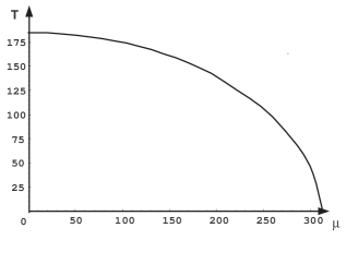
Figure 1: Plot of $T^{*}(\mu)$ in MeV, as obtained from Eq. (4) for $\Lambda=675$ MeV.

3 Fluctuation effects

In order to study the modifications to the mean field analysis it is necessary to introduce a method that can properly account for the fluctuation effects. Such approach has been developed Kleinert and van den Bossche (2000); Babaev (2000) and its essential features will be briefly illustrated in the following.

The four fermion interaction in the model in Eq. (1) can be cast in the form of Yukawa coupling, by introducing the auxiliary scalar and pseudoscalar fields $\sigma$ and $\vec{\pi}$:

$${\cal L}=\bar{\psi}(i\partial_{\nu}\gamma^{\nu}+\mu\gamma_{0}-g_{0}(\sigma+i\gamma_{5}{\vec{\tau}}\cdot{\vec{\pi}}))\psi-\frac{g_{0}^{2}N_{c}}{2G_{0}}\left[\sigma^{2}+{\vec{\pi}}^{2}\right]$$ (5)

with the quark-meson coupling constant given by $g_{0}=m_{q}/f_{\pi}$, which is the analogous of the Goldberger-Treiman relation. By functional integration of the fermionic degrees of freedom and derivative expansion, Eq. (5) becomes equivalent to the $\sigma$ model with lagrangian

$${\cal L}_{\sigma}=\frac{\beta}{2}\left((\partial\sigma)^{2}+(\partial{\vec{\pi}})^{2}-\frac{\kappa^{2}}{4}\left(\sigma^{2}+{\vec{\pi}}^{2}-f_{\pi}^{2}\right)^{2}\right)$$ (6)

where the stiffness parameter, $\beta$, which is relevant for our purposes, is given by Kleinert and van den Bossche (2000); Eguchi (1976)

$$\beta=4g_{0}^{2}N_{c}N_{f}\left(\int_{\Lambda}\frac{d^{4}p_{E}}{(2\pi)^{4}}\frac{1}{(p_{E}^{2}+m^{2}_{q})^{2}}-\frac{1}{2}\int_{\Lambda}\frac{d^{4}p_{E}}{(2\pi)^{4}}\frac{p_{E}^{2}}{(p_{E}^{2}+m^{2}_{q})^{3}}\right)$$ (7)

and $p_{E}$ is the Euclidean four-momentum.

The key point is that an equivalent description of the problem should be obtained by resorting to an effective theory, defined by a non-linear $\sigma$ model for the fields $\sigma$ and $\vec{\pi}$, satisfying the constraint $\sigma^{2}+{\vec{\pi}}^{2}\,=\,f_{\pi}^{2}$ Kleinert and van den Bossche (2000); Babaev (2000). This constraint can be introduced into the functional generator $Z$ of the non-linear $\sigma$ model, by means of a functional Lagrange multiplier $\lambda(x)$

$$Z=\int[d\sigma][d{\vec{\pi}}][d\lambda]\exp\left\{i\frac{\beta}{2}\int d^{4}x\left((\partial\sigma)^{2}+(\partial{\vec{\pi}})^{2}-\lambda\left(\sigma^{2}+{\vec{\pi}}^{2}-f_{\pi}^{2}\right)\right)\right\}$$ (8)

The parameter $\beta$ in Eq. (8) indicates the stiffness of the non-linear $\sigma$ model.

The functional integration of the $\vec{\pi}$ fields in Eq. (8) can be performed and, afterward, one can use the saddle point approximation and search for $x$-independent solutions for $\sigma$ and $\lambda$. As it is evident from Eq. (8), the constant $\lambda$ plays the role of a square mass both for $\sigma$ and $\vec{\pi}$ fields. Since we are looking for phase transitions at finite $T$ and $\mu$, we consider Matsubara frequencies $\tilde{\omega}_{n}=2\pi nT$ and non-vanishing baryonic chemical potential and the two saddle point conditions read

$$0=\lambda\sigma\;;\hskip 30.0pt0=\beta(f_{\pi}^{2}-\sigma^{2})-(N_{f}^{2}-1)\,\sum_{n=-\infty}^{\infty}\int_{\Lambda_{\pi}}\frac{d^{3}k}{(2\pi)^{3}}\frac{T}{(\tilde{\omega}_{n}-i\mu)^{2}+k^{2}+\lambda}$$ (9)

where $\Lambda_{\pi}$ is a suitable cutoff for the non-linear $\sigma$ model.

The first condition $0=\lambda\sigma$ indicates that at least one of the two variables must vanish and the other variable is implicitly determined from the second condition in Eq. (9), in terms of $T$, $\mu$ and of the stiffness $\beta$. The equivalence of the non-linear $\sigma$ model with the lagrangian in Eq. (6) implies that the stiffness evaluated in the two cases must coincide. Therefore one can insert the expression of $\beta$ of Eq. (7), properly modified to account for the finite $T$ and $\mu$ effects, i.e.

$$\beta=2g_{0}^{2}N_{f}N_{c}T\sum_{n=-\infty}^{+\infty}\int_{\Lambda}\frac{d^{3}p}{(2\pi)^{3}}\left[\frac{1}{[\epsilon^{2}+(\omega_{n}-i\mu)^{2}]^{2}}+\frac{m^{2}_{q}(T,\mu)}{[\epsilon^{2}+(\omega_{n}-i\mu)^{2}]^{3}}\right]$$ (10)

into Eq. (9) and determine the corresponding solution for $\sigma$ or $\lambda$.

As an example, in fig. 2 we plot the solutions of Eq. (9): $\sigma$ and the mass of the pionic mode $m_{\pi}=\sqrt{\lambda}$ versus the temperature, at $\mu=0$ and for two different values of the number of colors: $N_{c}=3$ (solid lines) and $N_{c}=10$ (dashed lines). The values of the two cutoffs entering Eqs. (9) and (10) are $\Lambda_{\pi}=200$ MeV and $\Lambda=675$ MeV. In fact $\Lambda_{\pi}$ and $\Lambda$ are related to different degrees of freedom and do not need to have the same value and we take a value of $\Lambda_{\pi}$ close to $f_{\pi}$, which fixes the scale of the non-linear $\sigma$ model. (The choice $\Lambda_{\pi}\sim\Lambda$ made in Hatsuda and Kunihiro (1985) has been criticized in Kleinert and van den Bossche (2000). For other references on this point see Castorina et al. (2005).)

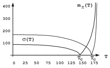
Figure 2: $\sigma$ and $m_{\pi}$ vs. $T$ at $\mu=0$ (in MeV) as obtained from Eq. (9). See text for the specific values of the other parameters.

We observe in fig. 2 that at low temperatures the solution of Eq. (9) corresponding to $\lambda=0$ (not plotted) and non-vanishing $\sigma$ is realized. Then $\sigma$ decreases with $T$ and eventually vanishes. By further increasing the temperature, the solution $\sigma=0$ (not plotted) and $m_{\pi}=\sqrt{\lambda}\neq 0$ is realized.

The two regions meet at $T=T_{c}$ where $\sigma=\lambda=0$. This corresponds in Eq. (9) to the critical stiffness

$$\beta_{c}=\frac{N_{f}^{2}-1}{f_{\pi}^{2}(T_{c},\mu)}\,\sum_{n=-\infty}^{\infty}\int_{\Lambda_{\pi}}\frac{d^{3}k}{(2\pi)^{3}}\frac{T_{c}}{(\tilde{\omega}_{n}-i\mu)^{2}+k^{2}}$$ (11)

and $T_{c}$ is determined by the comparison of Eqs. (10) and (11) In the particular case considered in fig. 2 we get $T_{c}\approx 146$ MeV for $N_{c}=3$ and $T_{c}\approx 172$ MeV for $N_{c}=10$.

One should notice that in the non-linear $\sigma$ model the region below $T_{c}$ shows a non-vanishing expectation value of the field $\sigma$ which implies a dynamical breaking of the chiral symmetry. Above $T_{c}$ this expectation value vanishes and at the same time a finite mass for the pions is generated. The absence from the spectrum of massless Goldstone bosons is a signal of chiral symmetry restoration. Therefore, within this framework, $T_{c}$ is the critical temperature related to the chiral symmetry.

In fig. 2, when the temperature is increased, $m_{\pi}$ grows and, at some temperature, $T_{pair}$, eventually diverges and the $\vec{\pi}$ mesons decouple and disappear from the spectrum. Reasonably, $T_{pair}$ could be interpreted as the temperature of dissociation of the $\bar{q}q$ pair. A remarkable feature which appears in fig.2 is that $T_{pair}$ does not depend on $N_{c}$ and, in practice, it numerically coincides with the critical temperature $T^{*}$ determined by the mean field analysis: $T_{pair}\sim T^{*}\sim 185$ MeV.

Therefore, the comparison of the NJL model with the non-linear $\sigma$ model indicates that fluctuations indeed modify the mean field conclusions and the new critical temperature $T_{c}$, associated with the chiral symmetry restoration, is generated. $T_{c}$ turns out to be smaller than $T^{*}$ so that we find a temperature interval $T_{c}<T<T^{*}$ where the gap equation still provides $m_{q}\neq 0$ but the chiral symmetry is restored as an effect of the fluctuations. Only above $T^{*}\sim T_{pair}$ the mesons disappear and $m_{q}$ vanishes. Consistently with this picture we note that $T_{c}$ depends on $N_{c}$ and $T_{c}\to T^{*}$ when $N_{c}\to\infty$, i.e. when the fluctuation effects become suppressed and the mean field regime holds.

A comment about $m_{q}$ is in order. In fact the common belief is that a non-vanishing $m_{q}$ is directly related to the breakdown of chiral symmetry. This is true only if the gap $m_{q}$ appears as a pole in the two point function of the fermion $\psi$. In our specific case $m_{q}$ corresponds to the pole mass of $\psi$ only in the mean field approximation. This property has been first observed in 2D models in Witten (1978), and, for a detailed treatment of the problem, we refer to Nikolov et al. (1996); Gusynin et al. (1999). With a suitable change of variables, corresponding to the introduction of polar ’coordinates’: $\sigma+i\gamma^{5}\pi=\rho~{}{\rm exp}(i\gamma^{5}\theta)$ and of the fermion $\chi={\rm exp}(i\gamma^{5}\theta/2)$, where $\rho$ and $\chi$ are chirally neutral, it is possible to show that $m_{q}$, as obtained from the gap equations (2) and (4) is a pole in the $\chi$ two point function (of course in our specific case the definition of the new variables should be modified to account for the flavor degrees of freedom). Due to the chiral neutrality of $\chi$, this excitation does not break chiral symmetry. Conversely, it does not appear in the $\psi$ propagator as a pole but rather, due to the $\theta$ field fluctuations, as a branch cut. In this sense, a finite $m_{q}$ is still compatible with chiral symmetry.

The presence of a region between two characteristic temperatures where the fluctuations cancel the long range order associated to the quark mass, restoring the symmetry, shows a clear resemblance with the pseudogap phase of high temperature superconductors Hatsuda and Kunihiro (1985); Kleinert and van den Bossche (2000); Gusynin et al. (1999) and this motivates the following analysis of the spectral function.

4 Evaluation of the pseudogap

After having determined the two characteristic temperatures $T_{c}$ and $T^{*}$, we conclude by showing that a simple approximation in the calculation of the spectral function provides clear indications of a pseudogap Castorina et al. (2005). The spectral function of the fermionic quasiparticles, $N(\omega)$, is obtained from the imaginary part of $G^{R}({\vec{k}},\omega)$:

$$N(\omega)=-\frac{1}{\pi}\int\frac{d{\vec{k}}}{(2\pi)^{3}}{\rm Tr}_{c,f,d}~{}~{}\gamma^{0}~{}{\rm Im}~{}G^{R}({\vec{k}},\omega)$$ (12)

where ${\rm Tr}_{c,f,d}$ is the trace over Dirac, color and flavor degrees of freedom. $G^{R}({\vec{k}},\omega)$ is the analytical continuation of the imaginary time retarded Green function: $G^{R}({\vec{k}},\omega)=\left[G^{-1}({\vec{k}},\omega+i\epsilon)-\Sigma_{R}({\vec{k}},\omega)\right]^{-1}$ where $G^{-1}({\vec{k}},\omega+i\epsilon)$ corresponds to the free term contribution and $\Sigma_{R}({\vec{k}},\omega)$ includes higher order corrections. The starting point to calculate the retarded Green function is the Lagrangian

$${\cal L}_{eff}=\bar{\psi}[i\partial_{\nu}\gamma^{\nu}+\mu\gamma_{0}-g_{0}(\sigma+i\gamma_{5}{\vec{\tau}}\cdot{\vec{\pi}})]\psi-\frac{g_{0}^{2}N_{c}}{2G_{0}}\left[\sigma^{2}+{\vec{\pi}}^{2}\right]$$ (13)

where the $\sigma$ field is replaced by expanding the constraint : $\sigma=\left(f_{\pi}^{2}-{\vec{\pi}}^{2}\right)^{1/2}\sim f_{\pi}-{\vec{\pi}}^{2}/(2f_{\pi})$. The correction $\Sigma_{R}({\vec{k}},\omega)$ to the free fermion propagator is computed to the one loop level from Eq. (13), Eguchi (1976), and its imaginary part generates the correction, $N_{pert}$, to the free fermion contribution in the spectral function

$$N(\omega)=\frac{N_{c}N_{f}}{\pi^{2}}(\omega+\mu)\sqrt{(\omega+\mu)^{2}-m_{q}^{2}}+N_{pert}\;.$$ (14)

In fact we have included the mass $m_{q}$, which is dynamically generated, in the free fermion contribution and we have also included in the definition of $g_{0}$ the form factor $g_{0}^{2}({\vec{q}}^{2})=g_{0}^{2}\,{m_{P}^{4}}/\left({m^{2}_{P}+(2\pi nT)^{2}+{q}^{2}}\right)^{2}$ with $m_{P}=100$ MeV, which acts as a regulator that corrects the large momentum behavior of the loop.

We normalize $N(\omega)$ to the free massless case : $R(\omega)=N(\omega)/(\frac{N_{c}N_{f}}{\pi^{2}}(\omega+\mu)^{2})$ and plot $R(\omega)$ for $(T-T_{c})/T_{c}=0.02,0.15,0.20$ ($\mu=10$ MeV) in fig. 3. The solid straight line corresponds to $T=T^{*}$. In fig. 3 we observe the pseudogap for values of $\omega$ just above the value $\omega=m_{q}-\mu$, where the free part of $N(\omega)$ vanishes, whereas it disappears for large values of $\omega$. The effect of the pseudogap is larger for temperatures just greater than $T_{c}$ and vanishes at $T=T^{*}$. Therefore, even in this simple approximation, it is possible to realize the presence of the depletion of states in the spectral function and this calculation supports the picture of a pseudogap appearing between the two characteristic temperatures. Since the NJL model effectively contains many ingredients of QCD, this analysis is a starting point to check the existence of a pseudogap in QCD and its possible role in the explanation of the mesonic bound states observed in lattice calculations.

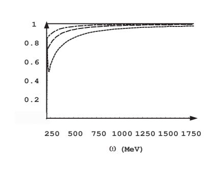
Figure 3: The ratio $N(\omega)/N_{free}(\omega)$ as a function of the energy $\omega$, at $\mu=10$ MeV and for various temperatures between $T_{c}$ and $T^{*}$. See text.

References

- Karsch (2005) F. Karsch (2005), hep-lat/0502014.
- Emery and Kivelson (1995) V. J. Emery, and S. A. Kivelson, Nature 374, 434 (1995).
- Hatsuda and Kunihiro (1985) T. Hatsuda, and T. Kunihiro, Phys. Rev. Lett. 55, 158–161 (1985).
- Kleinert and van den Bossche (2000) H. Kleinert, and B. van den Bossche, Phys. Lett. B474, 336–346 (2000), hep-ph/9907274.
- Babaev (2000) E. Babaev, Phys. Rev. D62, 074020 (2000), %****␣zappala.bbl␣Line␣25␣****hep-ph/0006087.
- Castorina et al. (2005) P. Castorina, G. Nardulli, and D. Zappala (2005), hep-ph/0505089.
- Nambu and Jona-Lasinio (1961a) Y. Nambu, and G. Jona-Lasinio, Phys. Rev. 122, 345–358 (1961a).
- Nambu and Jona-Lasinio (1961b) Y. Nambu, and G. Jona-Lasinio, Phys. Rev. 124, 246–254 (1961b).
- Klevansky (1992) S. P. Klevansky, Rev. Mod. Phys. 64, 649–708 (1992).
- Hatsuda and Kunihiro (1994) T. Hatsuda, and T. Kunihiro, Phys. Rept. 247, 221–367 (1994), hep-ph/9401310.
- Eguchi (1976) T. Eguchi, Phys. Rev. D14, 2755 (1976).
- Witten (1978) E. Witten, Nucl. Phys. B145, 110 (1978).
- Nikolov et al. (1996) E. N. Nikolov, W. Broniowski, C. V. Christov, G. Ripka, and K. Goeke, Nucl. Phys. A608, 411–436 (1996), hep-ph/9602274.
- Gusynin et al. (1999) V. Gusynin, V. Loktev, and S. Sharapov, JETP 88, 685 (1999).