Unified Theory of Elementary Particles
– in Search of Extra Dimensions –

Abstract

Even though the unified theory of electroweak interactions is very successful at low energies, there remains one part to be confirmed. It is the sector involving Higgs particles. Those Higgs particles are expected to be discovered. It has been shown recently that Higgs particles can be viewed as gauge fields in higher dimensional gauge theory. The mass of a Higgs particle and its coupling to other particles are constrained by the gauge principle. In this scenario the mass of a Higgs particle is predicted to be in the range of 120 GeV - 290 GeV, exactly in the range explored at LHC, provided that the extra dimension is curved and warped. Thus physics of extra dimensions can manifest itself in collider experiments at the LHC energies.

1 Unification in extra dimensions

At the most fundamental level quarks and leptons interact with each other by exchanging gauge bosons. Strong interactions are described by $SU(3)_{C}$ color gauge interactions whereas electroweak interactions by $SU(2)_{L}\times U(1)_{Y}$ gauge interactions. The associated gauge bosons are gluons, $W$ bosons, $Z$ bosons, and photons. There is one more field necessary to make the standard model of elementary particles to work. It is the Higgs field which not only spontaneously breaks the electroweak symmetry $SU(2)_{L}\times U(1)_{Y}$ to the electromagnetic symmetry $U(1)_{EM}$, but also gives fermions finite masses. There appear many parameters whose values are chosen to fit the observed data. There is no principle regulating the Higgs sector of the standard model.

This seemingly awkward dilemma is resolved in higher dimensional gauge theory. Long time ago Kaluza and Klein proposed an intriguing scenario in which we are living in five-dimensional spacetime.[1] They assumed that our spacetime is close to the product of four-dimensional Minkowski spacetime ($M_{4}$) and a circle ($S^{1}$) with a radius $R$. The metric in the five-dimensional space, $g_{MN}$ ($M,N=0,\cdots,4$), decomposes into the four-dimensional metric $g_{\mu\nu}$ ($\mu,\nu=0,\cdots,3$), the off-diagonal components $g_{\mu 4}$, and $g_{44}$. The general coordinate invariance in the fifth dimension implies that the $g_{\mu 4}$ components behave as four-dimensional elecromagnetic gauge potential $A_{\mu}$. In this manner the four-dimensional gravity and electromagnetism are unified in the five-dimensional gravity.

Motivated by Kaluza and Klein’s idea, we consider non-Abelian gauge theory in five-dimensional spacetime. Gauge potential decomposes into two parts;

$$\quad A_{M}=(~{}A_{\mu}~{},~{}A_{y}~{})~{}.$$ (1)

On $M_{4}\times S^{1}$, for instance, fields are expanded in Fourier series in the fifth coordinate $y$;

$$\quad A_{M}(x,y)=\sum_{n=-\infty}^{\infty}A_{M}^{(n)}(x)~{}e^{iny/R}~{}.$$ (2)

$A_{\mu}^{(0)}(x)$ describes four-dimensional gauge fields. $A_{y}^{(0)}(x)$ tranforms as a four-dimensional scalar. It is our contention that $A_{y}^{(0)}(x)$ contains the four-dimensional Higgs scalar field. Thus the Higgs field is a part of gauge fields and the unification of gauge fields and Higgs fields is achieved. The scenario is called the gauge-Higgs unification.[2,3]

2 Dynamical gauge-Higgs unification

To apply the gauge-Higgs unification scenario to the electroweak interactions, several ingredients must be implemented.

(i) In the electroweak theory $SU(2)_{L}\times U(1)_{Y}$ breaks down to $U(1)_{EM}$ and the Higgs fields transform as a doublet of the $SU(2)_{L}$ group. On the other hand, the extra-dimensional component of the gauge fields in the decomposition in (1) belongs to the adjoint representation of the gauge group. This means that one must begin with a larger group to achieve gauge-Higgs unification, as first clarified by Fairlie and by Manton.[2]

(ii) The electroweak symmetry is spontaneously broken by the 4-d Higgs fields, which are a part of the 5-d gauge fields. Dynamical electrowek symmetry breaking is induced by the Hosotani mechanism.[3,4] When the extra-dimensional space is non-simply connected, there appear non-Abelian generalization of the Aharonov-Bohm phases. Those non-Abelian Aharonov-Bohm phases, $\{\theta_{j}\}$, become dynamical degrees of freedom, even though they give vanishing field strengths at the classical level. At the quantum level those $\theta_{j}$, in general, develop nonvanishing expectation values, thus breaking the gauge symmetry.

(iii) Quarks and leptons are chiral in the electroweak theory. Left-handed and right-handed fermions interact with other particles differently. The most natural and powerful way of incorporating chiral fermions in higher dimensional theory is to have an orbifold in extra dimensions.[5] As a typical example, consider $M_{4}\times S^{1}$. An orbifold is obtained by identifying two points on $S^{1}$:

$(x^{\mu},y)\sim(x^{\mu},-y)$ .

The resultant spacetime is $M_{4}\times(S^{1}/Z_{2})$.

(iv) As is seen below, phenomenology emerging from dynamical gauge-Higgs unification in flat space contradicts with the observation. To have realistic phenomenology in Higgs particles, quarks, and leptons, extra-dimensional space should be curved. In particular, dynamical gauge-Higgs unification in the Randall-Sundrum warped space yields intriguing consequences which can be tested in the experiments at LHC.[6]

3 Extra dimensions : flat or curved?

One example in flat space with dynamical gauge-Higgs unification in electroweak interactions is given by the $U(3)_{S}\times U(3)_{W}$ model.[7] There are two relevant non-Abelian AB phases ($\theta_{1},\theta_{2}$). The effective potential $V_{\rm eff}(\theta_{1},\theta_{2})$ is depicted in fig. 1. The abolute minimum is located at $(\theta_{1},\theta_{2})=(0,\pm 0.269\pi)$ so that the electroweak symmetry $SU(2)_{L}\times U(1)_{Y}$ breaks down to the electromagnetic symmetry $U(1)_{EM}$.

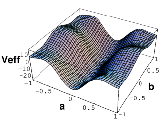
Figure 1: The effective potential for the non-Abelian AB phases ($\theta_{1}$=$\pi a\,$,$\,\theta_{2}$=$\pi b$) in the $U(3)_{S}\times U(3)_{W}$ model in flat space.

Although the symmetry is dynamically broken, there are two major problems. The $W$ boson mass is predicted to be $0.135/R$ where $R$ is the radius of extra-dimensins. It implies that the Kaluza-Klein mass scale $M_{KK}=1/R$ is about 600 GeV, which is too low. The mass of the Higgs particle is estimated from the curvature of the effective potential at its global minimum. One finds that $m_{H}\sim 0.871\times\sqrt{\alpha_{W}}\,m_{W}$ where $\alpha_{W}=g_{4}^{2}/4\pi$ is the weak fine structure constant. It leads to $m_{H}\sim 10$ GeV, contradicting with experimental data.

These two features are generic in flat space. The observational fact that the Higgs mass should be much bigger than $m_{W}$ indicates that the extra-dimensional space, if it exsits, must be curved.

The most promising spacetime in the context of dynamical gauge-Higgs unification is the Randall-Sundrum (RS) warped spacetime.[8,9] It has the same topology as $M_{4}\times(S^{1}/Z_{2})$. The metric is given by

$$ds^{2}=e^{-2\sigma(y)}dx_{\mu}dx^{\mu}+dy^{2}~{},$$ (3)

$$\sigma(y)=k|y|\quad\hbox{for }|y|\leq\pi R~{},$$ (4)

$$\sigma(y+2\pi R)=\sigma(y)~{}.$$ (5)

As in $M_{4}\times(S^{1}/Z_{2})$, $(x^{\mu},y)$ and $(x^{\mu},-y)$ are identified. It is the anti-de Sitter space with a cosmological constant $-1/k^{2}$ sandwitched by two branes at $y=0$ and $y=\pi R$. It has been speculated that five-dimensional anti-de Sitter space naturally emerges from such a more fundamental theory as superstring theory. Further reduction to four dimensions yields approximately conformal theory with gauge fields and light fermions.

The RS spacetime is specified with two parameters, $k$ and $R$. It is natural to suppose that the structure of spacetime is determined at the Planck scale $M_{pl}=1.2\times 10^{19}$ GeV. As a consequence it is expected that $k=O(M_{pl})$. The size $R$ is determined such that the theory predicts $m_{W}=80.4$ GeV. As is shown below, it implies that $kR=12\pm 0.3$.

4 $W$ bosons and the Kaluza-Klein mass

Consider $SU(3)$ gauge group which contains $SU(2)_{L}\times U(1)_{Y}$. Boundary conditions for the gauge fields in the RS spacetime (5) are given by

$$\hskip-5.69046pt\pmatrix{A_{\mu}\cr A_{y}}(x,y_{j}-y)=P_{j}\pmatrix{A_{\mu}\cr-A_{y}}(x,y_{j}+y)P_{j}^{\dagger}~{},$$ (6)

$$\hskip 28.45274pty_{0}=0~{},~{}y_{1}=\pi R~{},$$ (7)

$$\hskip 28.45274ptP_{0}=P_{1}=\pmatrix{-1\cr&-1\cr&&+1}~{}.$$ (8)

With these boundary conditions zero modes (massless modes) of $A_{M}$ in four dimensions exist only for components

$$\quad A_{\mu}=\pmatrix{\circ&\circ\cr\circ&\circ\cr&&\circ}~{},~{}A_{y}=\pmatrix{&&\circ\cr&&\circ\cr\circ&\circ}$$ (9)

where $\circ$ is marked. The zero modes of $A_{\mu}$ are $W$ bosons, $Z$ bosons, and photons, whereas those of $A_{y}$ constitute the Higgs doublet. In particular, the zero mode of $A_{y}$ gives rise to non-Abelian Aharonov-Bohm phase $\theta_{W}$:

$$\exp\bigg{\{}{\displaystyle i\over\displaystyle 2}\theta_{W}\Lambda\bigg{\}}=P\exp\bigg{\{}ig\int_{0}^{\pi R}dy\,\raise 0.68889pt\hbox{$\langle$}\lower 0.68889pt\hbox{}A_{y}\,\raise 0.68889pt\hbox{$\rangle$}\lower 0.68889pt\hbox{}\bigg{\}}~{},$$ (10)

$$\raise 0.68889pt\hbox{$\langle$}\lower 0.68889pt\hbox{}A_{y}\,\raise 0.68889pt\hbox{$\rangle$}\lower 0.68889pt\hbox{}=ce^{2ky}~{}\Lambda~{}~{},~{}~{}\Lambda=\pmatrix{\cr&&1\cr&1}~{}.$$ (11)

When $\theta_{W}\not=0$ ($mod~{}2\pi$), the $SU(2)_{L}$ symmetry breaks down and $W$ bosons acquire a mass $m_{W}$ given by

$$\quad m_{W}\sim\sqrt{{\displaystyle 2k\over\displaystyle\pi R}}~{}e^{-\pi kR}~{}\sin{\displaystyle\theta_{W}\over\displaystyle 2}~{}.$$ (12)

In the RS warped space the Kaluza-Klein mass scale $M_{KK}$, characterizing a mass spectrum $m_{n}\sim nM_{KK}$ is given by

$$\quad M_{KK} \sim {\displaystyle\pi k\over\displaystyle e^{\pi kR}-1}$$ (13)

$$= \cases{1/R&for $k\rightarrow 0$\cr\pi ke^{-\pi kR}&for $kR>2$~{}.\cr}$$ (14)

In a typical model $\theta_{W}$ takes a value $(0.2\pi\sim 0.5\pi)$. To yield $k=M_{pl}$ in (12), $kR$ must be $(11.75\sim 12.0)$. Note that $kR=6$ and 24 yield $k=10^{11}$ GeV and $10^{36}$ GeV, respectively. Thus the value of $kR$ is determined to be $12\pm 0.3$.

Combining (12) and (14), one obtains

$$\quad M_{KK}\sim{\displaystyle\pi\over\displaystyle\sin\hbox{${1\over 2}$}\theta_{W}}\bigg{(}{\displaystyle\pi kR\over\displaystyle 2}\bigg{)}^{1/2}m_{W}~{}.$$ (15)

This should be compared with the formula in flat space; $M_{KK}\sim(2\pi/\theta_{W})m_{W}$. There appears an enhancement factor $\hbox{${1\over 2}$}\pi kR\sim 20$ in the RS warped space. Inserting the value for $kR$, one finds that

$$\quad M_{KK}=1.6~{}{\rm TeV}\sim 3.6~{}{\rm TeV}~{}.$$ (16)

At LHC, Kaluza-Klein excited states can be produced in intermediate processes so that their existence can be indirectly checked for the value in (16).

5 Higgs particles

The Higgs field $\phi$ in four dimensions corresponds to fluctuations of the non-Abelian Aharonov-Bohm phase $\theta_{W}$. More explicitly

$$\quad\theta_{W}\rightarrow g_{4}\bigg{(}{\displaystyle\pi kR\over\displaystyle 2}\bigg{)}^{1/2}~{}{\displaystyle v+\phi\over\displaystyle M_{KK}}$$ (17)

where $g_{4}$ is the four-dimensional gauge coupling constant.

At the quantum level the effective potential for $\theta_{W}$ becomes nontrivial. Expanding it around its global minimum, one finds

$$\quad V_{\rm eff}(\theta_{W}) = {\rm const.}+{\displaystyle m_{H}^{2}\over\displaystyle 2}\phi^{2}$$ (19)

$$\hskip 14.22636pt+{\displaystyle\eta\over\displaystyle 3}\phi^{3}+{\displaystyle\lambda\over\displaystyle 4}\phi^{4}+\cdots~{}.$$

The effective potential is determined, once the mass spectrum $m_{n}(\theta_{W})$ is found for each field. It is shown that

$$\quad V_{\rm eff}(\theta_{W})={\displaystyle 3\over\displaystyle 128\pi^{6}}M_{KK}^{4}f(\theta_{W})$$ (20)

where $f(\theta_{W}+2\pi)=f(\theta_{W})$ is a periodic function with an amplitude of O(1).

It follows from (19) and (20) that

$$\quad m_{H}=\sqrt{{\displaystyle 3\alpha_{W}\over\displaystyle 32\pi}f^{(2)}(\theta_{W})}~{}{\displaystyle\pi kR\over\displaystyle 2}{\displaystyle m_{W}\over\displaystyle\sin\hbox{${1\over 2}$}\theta_{W}}$$ (21)

and

$$\quad\lambda={\displaystyle\alpha_{W}^{2}\over\displaystyle 16}f^{(4)}(\theta_{W})\bigg{(}{\displaystyle\pi kR\over\displaystyle 2}\bigg{)}^{2}$$ (22)

where $\alpha_{W}=g_{4}^{2}/4\pi\sim 0.03$. Notice the appearance of the enhancement factor $\hbox{${1\over 2}$}\pi kR$ in (21) and (22), which distinguishes the formulas in the warped space from those in flat space. In a typical model we have found that $f^{(2)}(\theta_{W})$ and $f^{(4)}(\theta_{W})$ are about 4. For $\theta_{W}=(0.2\sim 0.5)\pi$, one finds $m_{H}=(125\sim 286)$ GeV! (The experimental bound is $m_{H}>116$ GeV.[10]) It is remarkable that the dynamical gauge-Higgs unification predicts the mass of the Higgs particle exactly in the range where experiments at LHC will explore. The quartic coupling constant $\lambda$ is predicted to be $\sim 0.09$, though there is ambiguity in the value of $f^{(4)}(\theta_{W})$.

We summarize the prediction for $M_{KK}$, $m_{H}$, and $\lambda$ in Table 1. The values for $M_{KK}$ and $m_{H}$ predicted in flat space are inconsistent with the observation, but the situation drastically changes for the better in the Randall-Sundrum warped space.

	flat space	RS space
$M_{KK}$	$320\sim 800$ GeV	$1.6\sim 3.5$ TeV
$m_{H}$	$6\sim 15$ GeV	$125\sim 286$ GeV
$\lambda$	0.00025	0.09

Table 1: Prediction in the dynamical gauge-Higgs unification scenario in flat space and in the Randall-Sundrum warped space. $\theta_{W}$ is chosen to be $0.2\pi\sim 0.5\pi$.

6 Quarks and leptons

Another magic in the RS warped space appears in the fermion sector.[11] Each multiplet of fermions enters as a 5-d Dirac fermion in a triplet representation of $SU(3)$. For instance, a lepton multiplet $\psi$ in the first generation consists of

$$\quad\psi_{L}=\pmatrix{\nu_{L}\cr e_{L}\cr\tilde{e}_{L}}~{},~{}\psi_{R}=\pmatrix{\tilde{\nu}_{R}\cr\tilde{e}_{R}\cr e_{R}}~{}.$$ (23)

The components $\nu_{L}$, $e_{L}$, and $e_{R}$ have zero modes which appear as 4-d $\nu_{L}$, $e_{L}$, and $e_{R}$. On the other hand $\tilde{\nu}_{R}$, $\tilde{e}_{R}$, and $\tilde{e}_{L}$ have no zero modes so that they drop from the particle spectrum in four dimensions at low energies.

The Lagrangian density for a fermion multiplet in the RS space is given by

$${\mathcal{L}} = \psi\kern-6.49994pt\raise 6.00006pt\hbox{$-$}i\Gamma^{a}{e_{a}}^{M}D_{M}\psi-c\,k\,\psi\kern-6.49994pt\raise 6.00006pt\hbox{$-$}\psi~{},$$ (24)

$$\quad D_{M} = \partial_{M}+\frac{1}{8}\omega_{bcM}[\Gamma^{b},\Gamma^{c}]-igA_{M}~{}.$$ (25)

The covariant derivative $D_{M}$ is dictated by the general coordinate invariance and the gauge invariance. $ck\psi\kern-6.49994pt\raise 6.00006pt\hbox{$-$}\psi$ is called the bulk kink mass term.[12] $c$ is a dimensionless parameter.

Although $c$ is called a bulk mass parameter, quarks and leptons remain massless even with $c\not=0$ unless the electroweak symmetry breaks down. Their wave functions in the fifth dimension, however, depend on the value $c$. When the electroweak symmetry breaks down with nonvanishing $\theta_{W}$, those quarks and leptons acquire finite masses given by

$$m_{f}=\sqrt{{\displaystyle\pi kR\over\displaystyle 2}{\displaystyle(1-4c^{2})(z_{1}^{2}-1)\over\displaystyle(z_{1}^{1-2c}-1)(z_{1}^{1+2c}-1)}}~{}m_{W}$$ (26)

where $z_{1}=e^{\pi kR}$. A fermion mass is determined by $c$, or vice versa. See fig. 2.

$c=\pm\hbox{${1\over 2}$}$ corresponds to $m_{f}=m_{W}$. Except for top quarks all fermions have $|c|>\hbox{${1\over 2}$}$. As shown in Table 2, the top quark mass corresponds to $c=0.43$ whereas the electron mass to $c=0.87$. Although $m_{t}/m_{e}\sim 10^{5}$, there appears no hierarchical structure in the $c$ space. This gives us a good hint to understand the hierarchy in the quark-lepton mass spectrum.

Figure 2: The bulk mass parameter $c$ v.s. the fermion mass $m_{f}$ in (26).

particle	mass (GeV)	$c$
$e$	$0.510\times 10^{-3}$	$0.87$
$\mu$	$0.105$	$0.72$
$\tau$	$1.777$	$0.63$
$u$	$4\times 10^{-3}$	$0.81$
$c$	$1.3$	$0.64$
$t$	$175$	$0.43$

Table 2: The bulk kink mass parameter $c$ for each quark or lepton, following from (26)

7 Outlook

The results obtained in the dynamical gauge-Higgs unification in the Randall-Sundrum warped spacetime are surprising. The mass of the Higgs particle is predicted in the range 125 GeV to 285 GeV. We have determined the fermion wave functions in terms of their masses, with which couplings of quarks and leptons to the KK excited states of $W$ bosons etc. can be determined. In the LHC experiments we might be able to see the trace of the extra dimension, directly or indirectly.

8 Acknowledgement

This work was financially supported by the Japanese Ministry of Education and the 21st Century COE Program at Osaka University, “Towards a New Basic Science: Depth and Synthesis”.

References

- (1) Th. Kaluza, Sitzungsber, Preuss. Akad. Wiss. Berlin, Phys. Math. Klasse (1921) 966; O. Klein, Z. Phys. 37 (1926) 895.
- (2) D.B. Fairlie, Phys. Lett. B82 (1979) 97; N. Manton, Nucl. Phys. B158 (1979) 141.
- (3) Y. Hosotani, Phys. Lett. B126 (1983) 309; Ann. Phys. (N.Y.) 190 (1989) 233.
- (4) Y. Hosotani, in the Proceedings of “Dynamical Symmetry Breaking”, Nagoya University, December 2004, page 17. (arXiv:hep-ph/0504272)
- (5) A. Pomarol and M. Quiros, Phys. Lett. B438 (1998) 255.
- (6) Y. Hosotani and M. Mabe, Phys. Lett. B615 (2005) 257.
- (7) Y. Hosotani, S. Noda and K. Takenaga, Phys. Lett. B607 (2005) 276.
- (8) L. Randall and R. Sundrum, Phys. Rev. Lett. 83 (1999) 3370.
- (9) K. Oda and A. Weiler, Phys. Lett. B606 (2005) 408.
- (10) LEP Electroweak Working Group, http://lepewwg.web.cern.ch/lepewwg/ .
- (11) Y. Hosotani, S. Noda and Y. Sakamura, and S. Shimasaki, in preparation.
- (12) T. Gherghetta and A. Pomarol, Nucl. Phys. B586 (2000) 141.