Supersymmetric Standard Model from the Heterotic String

Abstract

We present a $\mathbbm{Z}_{6}$ orbifold compactification of the $\mathrm{E}_{8}\times\mathrm{E}_{8}$ heterotic string which leads to the (supersymmetric) Standard Model gauge group and matter content. The quarks and leptons appear as three $\boldsymbol{16}$–plets of $\mathrm{SO}(10)$, whereas the Higgs fields do not form complete $\mathrm{SO}(10)$ multiplets. The model has large vacuum degeneracy. For generic vacua, no exotic states appear at low energies and the model is consistent with gauge coupling unification. The top quark Yukawa coupling arises from gauge interactions and is of the order of the gauge couplings, whereas the other Yukawa couplings are suppressed.

The problem of ultraviolet completion of the (supersymmetric) Standard Model (SM) has been a long–standing issue in particle physics. The most promising approach is based on string theory, however explicit models usually contain exotic particles and suffer from other phenomenological problems. The purpose of this Letter is to show that these difficulties can be overcome in the well known weakly coupled heterotic string ghx85 compactified on an orbifold dhx85 ; inx87 . The emerging picture has a simple geometrical interpretation.

In the light cone gauge the heterotic string can be described by the following bosonic world sheet fields: 8 string coordinates $X^{i}$, $i=1\ldots 8$, 16 internal left-moving coordinates $X^{I}$, $I=1\ldots 16$, and 4 right-moving fields $\phi^{i}$, $i=1\ldots 4$, which correspond to the bosonized Neveu-Schwarz-Ramond fermions (cf. kkx90 ). The 16 left-moving internal coordinates are compactified on a torus. The associated quantized momenta lie on the $\mathrm{E}_{8}\times\mathrm{E}_{8}$ root lattice. The massless spectrum of this 10D string is 10D supergravity coupled to $\mathrm{E}_{8}\times\mathrm{E}_{8}$ super Yang–Mills theory.

To get an effective four–dimensional theory, 6 dimensions of the 10D heterotic string are compactified on an orbifold. A $\mathbbm{Z}_{N}$ orbifold is obtained by modding a 6D torus together with the 16D gauge torus by a $\mathbbm{Z}_{N}$ twist, ${\cal O}\ =\ \mathbbm{T}^{6}\otimes\mathbbm{T}_{\mathrm{E}_{8}\times\mathrm{E}_{8}^{\prime}}/\mathbbm{Z}_{N}$. On the three complex torus coordinates $z^{i}$, $i=1,2,3$, the $\mathbbm{Z}_{N}$ twist acts as $z^{i}\rightarrow e^{2\pi\mathrm{i}\,v_{N}^{i}}~{}z^{i}$, where $Nv_{N}$ has integer components and $\sum_{i}v_{N}^{i}=0$. This action is accompanied by the shifts of the bosonized fermions $\phi^{i}$ and the gauge coordinates $X^{I}$, $\phi^{i}\rightarrow\phi^{i}-\pi v_{N}^{i}\;,\quad X^{I}\rightarrow X^{I}+\pi V_{N}^{I}$, where $NV_{N}$ is an $\mathrm{E}_{8}\times\mathrm{E}_{8}$ lattice vector. Further, if discrete Wilson lines $W^{I}_{l}$ are present inx87 , the torus lattice translations are accompanied by the shifts $X^{I}\rightarrow X^{I}+\pi n_{l}W^{I}_{l}$ with integer $n_{l}$. In addition to the requirement that $NV_{N}$ and $nW$, where $n$ is the order of the Wilson line, be $\mathrm{E}_{8}\times\mathrm{E}_{8}$ lattice vectors, $V_{N}$ and $W$ are constrained by modular invariance (cf. Kobayashi:2004ud ; Forste:2004ie ). At each fixed point of the orbifold, a local $\mathbbm{Z}_{N}$ twist, composed of $V_{N}$ and discrete Wilson lines, breaks $\mathrm{E}_{8}\times\mathrm{E}_{8}$ to a subgroup (cf. Buchmuller:2004hv ). Given an orbifold, a torus lattice together with the shift $V_{N}$ and the Wilson lines, the massless spectrum of the orbifold can be calculated. It is supersymmetric by construction and consists of the states which are invariant under the twisting and lattice translations.

Figure 1: $\mathrm{G}_{2}\times\mathrm{SU}(3)\times\mathrm{SO}(4)$ torus lattice of a $\mathbbm{Z}_{6}$-II orbifold.

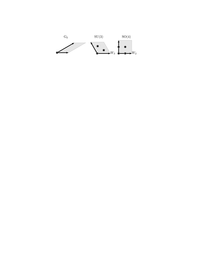
In our construction we choose a $\mathbbm{Z}_{6}$-II orbifold based on a Lie torus lattice $\mathrm{G}_{2}\times\mathrm{SU}(3)\times\mathrm{SO}(4)$ (Fig. 1) with a twist vector $v_{6}=\left(\frac{1}{6},\frac{1}{3},-\frac{1}{2}\right)$ Kobayashi:2004ud . In addition to $V_{6}$, we require two Wilson lines: one of order two in the $\mathrm{SO}(4)$ plane, and another of order three in the $\mathrm{SU}(3)$ plane. In an orthonormal basis, the shift and the Wilson lines are given by

$$V_{6} = \left(\tfrac{1}{2},\tfrac{1}{2},\tfrac{1}{3},0,0,0,0,0\right)\,\left(\tfrac{1}{3},0,0,0,0,0,0,0\right)\;,$$

$$W_{2} = \left(\tfrac{1}{2},0,\tfrac{1}{2},\tfrac{1}{2},\tfrac{1}{2},0,0,0\right)\,\left(-\tfrac{3}{4},\tfrac{1}{4},\tfrac{1}{4},-\tfrac{1}{4},\tfrac{1}{4},\tfrac{1}{4},\tfrac{1}{4},-\tfrac{1}{4}\right)\;,$$

$$W_{3} = \left(\tfrac{1}{3},0,0,\tfrac{1}{3},\tfrac{1}{3},\tfrac{1}{3},\tfrac{1}{3},\tfrac{1}{3}\right)\,\left(1,\tfrac{1}{3},\tfrac{1}{3},\tfrac{1}{3},0,0,0,0\right)\;.$$

The model has twelve fixed points which come in six inequivalent pairs, with the local groups

$$\begin{array}[]{l}\mathrm{SO}(10)\times\mathrm{SO}(4)\;,\;\mathrm{SO}(12)\;,\;\mathrm{SU}(7)\;,\\ \mathrm{SO}(8)\times\mathrm{SO}(6)\;,\;\mathrm{SO}(8)^{\prime}\times\mathrm{SO}(6)^{\prime}\;,\;\mathrm{SO}(8)^{\prime\prime}\times\mathrm{SO}(6)^{\prime\prime}\end{array}$$

up to $\mathrm{U}(1)$ factors and subgroups of the second $\mathrm{E}_{8}$. The standard model gauge group, $G_{\mathrm{SM}}=\mathrm{SU}(3)_{c}\times\mathrm{SU}(2)_{\mathrm{L}}\times\mathrm{U}(1)_{Y}$, is obtained as an intersection of those groups. The surviving gauge group in 4D is

$$G~{}=~{}G_{\mathrm{SM}}\times\left[\mathrm{SO}(6)\times\mathrm{SU}(2)\right]\times\mathrm{U}(1)^{8}\;,$$ (1)

where one of the $\mathrm{U}(1)$’s is anomalous, and the brackets indicate a subgroup of the second $\mathrm{E}_{8}$. The matter multiplets are found by solving the masslessness equations together with the twist- and translation–invariance conditions. The resulting spectrum includes both untwisted ($U$, “bulk”) and twisted ($T_{k}$, “localized”) states, and is given in Tab. 1. The twisted states can belong to any of the twisted sectors $T_{k}$ ($k=1,2,3,4$) depending on their string boundary conditions. There are no left–chiral superfields in the $T_{5}$ sector.

name Representation count name Representation count $q_{i}$ $(\boldsymbol{3},\boldsymbol{2};\boldsymbol{1},\boldsymbol{1})_{1/6}$ 3 $\bar{u}_{i}$ $(\overline{\boldsymbol{3}},\boldsymbol{1};\boldsymbol{1},\boldsymbol{1})_{-2/3}$ 3 $\bar{d}_{i}$ $(\overline{\boldsymbol{3}},\boldsymbol{1};\boldsymbol{1},\boldsymbol{1})_{1/3}$ 7 $d_{i}$ $(\boldsymbol{3},\boldsymbol{1};\boldsymbol{1},\boldsymbol{1})_{-1/3}$ 4 $\bar{\ell}_{i}$ $(\boldsymbol{1},\boldsymbol{2};\boldsymbol{1},\boldsymbol{1})_{1/2}$ 5 $\ell_{i}$ $(\boldsymbol{1},\boldsymbol{2};\boldsymbol{1},\boldsymbol{1})_{-1/2}$ 8 $m_{i}$ $(\boldsymbol{1},\boldsymbol{2};\boldsymbol{1},\boldsymbol{1})_{0}$ 8 $\bar{e}_{i}$ $(\boldsymbol{1},\boldsymbol{1};\boldsymbol{1},\boldsymbol{1})_{1}$ 3 $s^{-}_{i}$ $(\boldsymbol{1},\boldsymbol{1};\boldsymbol{1},\boldsymbol{1})_{-1/2}$ 16 $s^{+}_{i}$ $(\boldsymbol{1},\boldsymbol{1};\boldsymbol{1},\boldsymbol{1})_{1/2}$ 16 $s^{0}_{i}$ $(\boldsymbol{1},\boldsymbol{1};\boldsymbol{1},\boldsymbol{1})_{0}$ 69 $h_{i}$ $(\boldsymbol{1},\boldsymbol{1};\boldsymbol{1},\boldsymbol{2})_{0}$ 14 $f_{i}$ $(\boldsymbol{1},\boldsymbol{1};\boldsymbol{4},\boldsymbol{1})_{0}$ 4 $\bar{f}_{i}$ $(\boldsymbol{1},\boldsymbol{1};\overline{\boldsymbol{4}},\boldsymbol{1})_{0}$ 4 $w_{i}$ $(\boldsymbol{1},\boldsymbol{1};\boldsymbol{6},\boldsymbol{1})_{0}$ 5

Table 1: The $G_{\mathrm{SM}}\times[\mathrm{SO}(6)\times\mathrm{SU}(2)]$ quantum numbers of the spectrum.

Let us now discuss some properties of the spectrum. We first note that the $V_{6}$ shift is chosen such that the local gauge symmetry at the origin is $\mathrm{SO}(10)\times\mathrm{SO}(4)\times\mathrm{U}(1)$ and the twisted matter at this point is a $\boldsymbol{16}$–plet of $\mathrm{SO}(10)$ plus $\mathrm{SO}(10)$-singlets. When the $\mathrm{SU}(3)\times\mathrm{SU}(2)\times\mathrm{U}(1)\subset\mathrm{SO}(10)$ factor is identified with the SM group $G_{\mathrm{SM}}$ (with the standard GUT hypercharge embedding), the $\boldsymbol{16}$–plet of $\mathrm{SO}(10)$ gives a complete generation of the SM matter, including the right–handed neutrino. Since there are two equivalent fixed points in the $\mathrm{SO}(4)$ plane (Fig. 2), there are 2 copies of the $\boldsymbol{16}$–plets. Due to our choice of Wilson lines, the remaining matter has the SM quantum numbers of an additional $\boldsymbol{16}$–plet plus vector–like multiplets. This can partly be understood from the SM anomaly cancellation. Thus, we have

$$\text{matter:}~{}~{}~{}~{}3\times\boldsymbol{16}~{}~{}+~{}~{}\text{vector-like}\;.$$ (2)

Two generations are localized in the compactified space and come from the first twisted sector $T_{1}$, whereas the third generation is partially twisted and partially untwisted:

$$2\times\boldsymbol{16}\in T_{1}~{}~{},~{}~{}\boldsymbol{16}\in U,T_{2},T_{4}\;.$$ (3)

In particular, the up–quark and the quark doublet of the third generation are untwisted, which results in a large Yukawa coupling, whereas the down–quark is twisted and its Yukawa coupling is suppressed.

Figure 2: Local gauge symmetries in the $\mathrm{SO}(4)$ plane (at the origin in the $\mathrm{G}_{2}$ and $\mathrm{SU}(3)$ planes). Two $\boldsymbol{16}$–plets arise from the orbifold fixed points.

It is well known that the heterotic orbifold models have large vacuum degeneracy which gives enough freedom for realistic constructions Casas:1988se ; Font:1988mm ; Font:1989aj . There are many flat directions in the field space along which supersymmetry is preserved but some of the gauge symmetries are broken. In particular, all of the $\mathrm{U}(1)$ factors of Eq. (1) apart from the hypercharge are broken by giving vacuum expectation values (VEVs) along $D$– and $F$–flat directions to some of the 69 singlets $s^{0}_{i}$. We note that cancellation of the Fayet–Iliopoulos $D$–term associated with an anomalous $\mathrm{U}(1)$ requires that at least some of the VEVs be close to the string scale. Choosing all the singlet VEVs of order the string scale, the $\mathrm{U}(1)$ gauge bosons are decoupled, and we have

$$G~{}\longrightarrow~{}\mathrm{SU}(3)_{c}\times\mathrm{SU}(2)_{\mathrm{L}}\times\mathrm{U}(1)_{Y}\times G_{\mathrm{hidden}}\;,$$ (4)

with $G_{\mathrm{hidden}}=\mathrm{SO}(6)\times\mathrm{SU}(2)$. This leads to complete separation between the hidden and observable sectors.

One of the main problems of string models is the presence of exotic states at low energies. Generically, such states are inconsistent with experimental data and destroy gauge coupling unification. Even if the exotic states are vector–like with respect to the SM, they are still harmful unless they attain large masses. However, one cannot assign the mass terms at will. They must appear due to VEVs of some singlets and be consistent with string selection rules [Hamidi:1986vh, ,Font:1988mm, ]. In most cases, the latter prohibit many of the required couplings such that the exotic states stay light. One of the achievements of our model is that all of the exotic vector–like states can be given large masses consistently with string selection rules.

To proceed, let us briefly summarize these rules Kobayashi:2004ud . The coupling

$$\Psi_{1}\Psi_{2}\dots\Psi_{n}$$ (5)

between the states $\Psi_{i}$ belonging to twisted sectors $T_{k_{i}}$ (including also the untwisted sector) to be allowed, the total twist has to be a multiple of 6: $\sum_{i}k_{i}=0$ mod 6. There are further restrictions on the fixed points that can enter into this product, called a space group selection rule. For example, in the $\mathrm{SO}(4)$ plane it amounts to $\sum_{i}(n^{(i)},n^{(i)^{\prime}})=(0,0)$ mod 2, where $(n^{(i)},n^{(i)^{\prime}})$ are the coordinates of the fixed points in the orthonormal basis, $n^{(i)},n^{(i)^{\prime}}=\{0,1\}$. Similar rules apply to the $\mathrm{SU}(3)$ and the $\mathrm{G}_{2}$ planes. Further, there is a requirement of gauge invariance $\sum_{i}p_{i}=0$, where $p_{i}$ are the (shifted) momenta in the $\mathrm{E}_{8}\times\mathrm{E}_{8}$ gauge lattice. Finally, the $\boldsymbol{H}$–momentum in the compact 6D space must also be conserved, $\sum_{i}R_{1}^{(i)}=-1$ mod 6, $\sum_{i}R_{2}^{(i)}=-1$ mod 3, $\sum_{i}R_{3}^{(i)}=-1$ mod 2, where $R_{1,2,3}$ are the $\boldsymbol{H}$–momenta associated with the $\mathrm{G}_{2}$, $\mathrm{SU}(3)$ and $\mathrm{SO}(4)$ planes, respectively.

Based on these selection rules, we analyze allowed superpotential couplings involving vector–like pairs of exotic fields $x_{i}\bar{x}_{j}$ and the SM singlets $s_{a}$:

$$W=x_{i}\bar{x}_{j}\langle s_{a}s_{b}\dots\rangle\;.$$ (6)

We find that all of the exotic states enter such superpotential couplings. This requires a product of up to 6 singlets. In order to decouple the exotic states one has to make sure that the corresponding mass matrices have a maximal rank such that no massless exotic states survive. An interesting feature of the model is that there are exotic states with the SM quantum numbers of the right–handed down quarks and lepton doublets. As a result these extra states mix with those from the $\boldsymbol{16}$–plets of $\mathrm{SO}(10)$, such that the observed matter fields are a mixture of both (cf. Asaka:2003iy ,Casas:1988se ). In particular, for down–type quarks we have the following mass matrix:

$$\begin{array}[]{r|ccccccc}&\bar{d}_{1}&\bar{d}_{2}&\bar{d}_{3}&\bar{d}_{4}&\bar{d}_{5}&\bar{d}_{6}&\bar{d}_{7}\\ \hline\cr d_{1}&s^{5}&s^{5}&s^{5}&s^{5}&s^{5}&s^{3}&s^{3}\\ d_{2}&s^{1}&s^{1}&s^{3}&s^{3}&s^{3}&s^{3}&s^{3}\\ d_{3}&s^{1}&s^{1}&s^{3}&s^{3}&s^{3}&s^{3}&s^{3}\\ d_{4}&s^{6}&s^{6}&s^{6}&s^{3}&s^{3}&s^{6}&s^{6}\end{array}$$

Here $s^{n}$ indicates that the coupling appears when a product of $n$ singlets is included. Different entries with the same $n$ generally correspond to different mass terms since they involve different singlets and Yukawa couplings. This mass matrix has rank 4 reflecting the fact that only 3 down–type quarks survive and the others have large masses, e.g. of the order of the string scale. Note that higher $n$ does not necessarily imply suppression of the coupling: $\langle s\rangle$ can be close to the string scale and, furthermore, the combinatorial coefficient in front of the coupling grows with $n$.

An important phenomenological constraint on this texture comes from suppression of $R$–parity violating interactions. It turns out that, in order to prohibit $\bar{u}\bar{d}\bar{d}$ and similar couplings at the renormalizable level, the $\bar{d}_{6,7}$ component in the massless $\bar{d}$–quarks must be suppressed. This is achieved choosing appropriate directions in the space of singlet VEVs.

For the lepton/Higgs doublets we have

$$\begin{array}[]{l|cccccccc}&\ell_{1}&\ell_{2}&\ell_{3}&\ell_{4}&\ell_{5}&\ell_{6}&\ell_{7}&\ell_{8}\\ \hline\cr\bar{\ell}_{1}&s^{3}&s^{4}&s^{4}&s^{1}&s^{1}&s^{1}&s^{1}&s^{1}\\ \bar{\ell}_{2}&s^{1}&s^{2}&s^{2}&s^{5}&s^{5}&s^{3}&s^{3}&s^{3}\\ \bar{\ell}_{3}&s^{1}&s^{2}&s^{2}&s^{5}&s^{5}&s^{3}&s^{3}&s^{3}\\ \bar{\ell}_{4}&s^{1}&s^{2}&s^{2}&s^{5}&s^{5}&s^{6}&s^{3}&s^{3}\\ \bar{\ell}_{5}&s^{1}&s^{6}&s^{6}&s^{3}&s^{3}&s^{6}&s^{3}&s^{3}\end{array}$$

This matrix has rank 5 which results in 3 massless doublets of hypercharge $-1/2$ at low energies. In order to get an extra pair of (“Higgs”) doublets with hypercharge $-1/2$ and $1/2$, one has to adjust the singlet VEVs such that the rank reduces to 4. This unsatisfactory fine tuning constitutes the well known supersymmetric $\mu$–problem. A further constraint on the above texture comes from the top Yukawa coupling: it is order one if the up–type Higgs doublet has a significant component of $\bar{\ell}_{1}$.

From the flavour physics perspective, it is interesting that only the right–handed down–type quarks and the lepton/Higgs doublets mix with the exotic states. Implications of this phenomenon will be studied elsewhere. Finally, the remaining exotic states $m_{i}$ and $s_{i}^{\pm}$ have full rank mass matrices and can be decoupled as well.

We have checked that the above decoupling is consistent with vanishing of the $D$–terms. This is implemented by constructing gauge invariant monomials out of the singlets Buccella:1982nx involved in the mass terms for the exotic states. The $F$–flatness condition requires a more detailed study and will be discussed elsewhere. Let us only mention that there are plenty of $F$–flat directions in the field space, for example, any direction in the 39-dimensional space of $T_{2}$,- $T_{4}$- and $U$-sector non–Abelian singlets is $F$–flat to all orders as long as the singlets from $T_{1,3}$ have zero VEVs. This is enforced by the $\boldsymbol{H}$–momentum selection rule for the $\mathrm{SO}(4)$ plane. Whether the decoupling of all of the extra matter can be done using exactly flat directions or it requires isolated solutions to the $F_{i}=D_{a}=0$ equations is currently under investigation. In any case, one can show that $F_{i}=D_{a}=0$ can be satisfied simultaneously on certain low-dimensional manifolds in the field space, so the decoupling of extra matter can be done consistently with supersymmetry.

The string selection rules have important implications for the matter Yukawa couplings. In particular, in our setup the only large Yukawa coupling is that of the top quark. The reason is that, at the renormalizable level, the types of couplings allowed by the space group and the $\boldsymbol{H}$–momentum are $UUU$, $T_{1}T_{2}T_{3}$, $T_{1}T_{1}T_{4}$, $UT_{2}T_{4}$, $UT_{3}T_{3}$. The third generation up quark and quark doublet as well as the up–type Higgs doublet (up to a mixing) are untwisted, so there is an allowed Yukawa interaction of the type $UUU$ whose strength is given by the gauge coupling. The Yukawa couplings involving the $T_{3}$ sector vanish since there is no SM matter in that sector. The coupling $UT_{2}T_{4}$ is incompatible with the $\mathrm{SU}(2)_{\mathrm{L}}\times\mathrm{U}(1)_{Y}$ symmetry, while the coupling $T_{1}T_{1}T_{4}$ is prohibited due to either gauge invariance or decoupling of the exotic down–type quarks required by suppression of $R$–parity violation. Therefore, all quarks and leptons apart from the top quark are massless at the renormalizable level and their Yukawa interactions appear due to higher order superpotential couplings. These are suppressed when the involved singlets have VEVs below the string scale.

An important feature of the model is that it admits spontaneous supersymmetry breakdown via gaugino condensation Ferrara:1982qs . The $\mathrm{SO}(6)$ group of the hidden sector is asymptotically free and its condensation scale depends on the matter content. The $\boldsymbol{6}$–plets and the $\boldsymbol{4}$,$\overline{\boldsymbol{4}}$–plets of $\mathrm{SO}(6)$ can be given large masses consistently with the string selection rules. In this case, the condensation scale is in the range $\sim 10^{11}-10^{13}\,\mathrm{GeV}$ depending on the threshold corrections to the gauge couplings. Assuming that the dilaton is fixed via the Kähler stabilization mechanism Banks:1994sg , gaugino condensation translates into supersymmetry breaking by the dilaton. The scale of the soft masses, $m_{3/2}$, depends on the details of dilaton stabilization and can be in the TeV–range.

Since our model has no exotic states at low energies and admits TeV–scale soft masses, it is consistent with gauge coupling unification. Then a natural question to ask is what are the orbifold GUT limits Kobayashi:2004ud ; Forste:2004ie ; Buchmuller:2004hv of this model. That is, what is the effective field theory limit in the energy range between the compactification scale and the string scale when some of the compactification radii are significantly larger than the others. Such anisotropic compactifications may mitigate the discrepancy between the GUT and string scales, and can be consistent with perturbativity for one or two large radii of order $(2\times 10^{16}~{}{\rm GeV})^{-1}$ Witten:1996mz . In our model, the intermediate orbifold picture can have any dimensionality between 5 and 10. For example, the 6D orbifold GUT limits are (up to $\mathrm{U}(1)$ factors) :

$$\mathrm{SO}(4)~{}\text{plane} : ~{}\text{bulk GUT}=\mathrm{SU}(6)~{},~{}N=2\;,$$

$$\mathrm{SU}(3)~{}\text{plane} : ~{}\text{bulk GUT}=\mathrm{SU}(8)~{},~{}N=2\;,$$

$$\mathrm{G}_{2}~{}\text{plane} : ~{}\text{bulk GUT}=\mathrm{SU}(6)\times\mathrm{SO}(4)~{},~{}N=4\;,$$

where the plane with a “large” compactification radius is indicated and $N$ denotes the amount of supersymmetry. In all of these cases, the bulk $\beta$–functions of the SM gauge couplings coincide. This is because either $G_{\mathrm{SM}}$ is contained in a simple gauge group or there is $N=4$ supersymmetry. Thus, unification may occur below the string scale. (To check whether this is the case, logarithmic corrections from localized fields, contributions from vector–like heavy fields and string thresholds have to be taken into account.) The SM gauge group is obtained as an intersection of the gauge groups at the different fixed points of the 6D orbifold (Fig. 3).

Figure 3: A 6D orbifold GUT limit with a large $\mathrm{SO}(4)$–plane compactification radius.

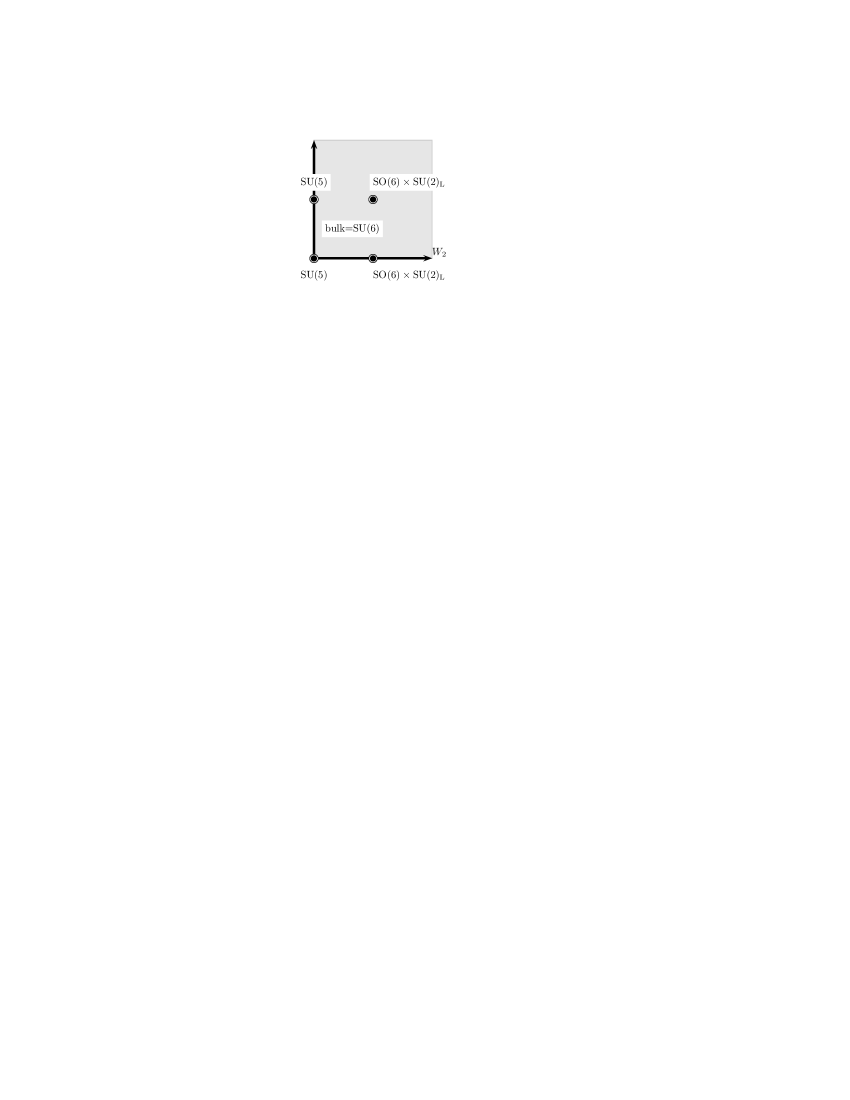
In this Letter, we have presented a heterotic string model which reproduces the spectrum of the minimal supersymmetric SM and is consistent with gauge coupling unification. The emerging picture has a simple geometrical interpretation. The SM gauge group is obtained as an intersection of the local $\mathrm{E}_{8}$ subgroups at inequivalent orbifold fixed points. Two generations of quarks and leptons appear as $\boldsymbol{16}$–plets localized at the fixed points with unbroken $\mathrm{SO}(10)$ symmetry, whereas the third ‘$\boldsymbol{16}$–plet’ involves both bulk and localized states. The Yukawa couplings do not exhibit $\mathrm{SO}(10)$ relations. The top quark Yukawa coupling is related to the gauge couplings, while the other Yukawa couplings are due to non–renormalizable interactions. The model has a hidden sector which allows for supersymmetry breaking via gaugino condensation.

Finally, let us remark that although this model is very special, it is perhaps not unique. In the $\mathbbm{Z}_{6}$-II orbifold with the $V_{6}$ shift given above, there are roughly $10^{4}$ models (some of them may be equivalent) with the SM gauge group. ${\cal O}(10^{2})$ of them have 3 matter generations plus vector–like exotic matter, whereas we have so far found only one model where the vector–like matter can be decoupled consistently with the string selection rules. We plan to investigate this issue further. It would also be interesting to understand the relation of this type of models to other phenomenologically promising constructions Braun:2005ux .

We thank T. Kobayashi, H. P. Nilles and S. Stieberger for valuable discussions. This work was partially supported by the European Union 6th Framework Program MRTN-CT-2004-503369 “Quest for Unification” and MRTN-CT-2004-005104 “ForcesUniverse”.

References

- (1) D. J. Gross et al., Phys. Rev. Lett. 54, 502 (1985); Nucl. Phys. B 256 (1985) 253.
- (2) L. J. Dixon et al., Nucl. Phys. B 261 (1985) 678; Nucl. Phys. B 274 (1986) 285.
- (3) L. E. Ibáñez, H. P. Nilles, F. Quevedo, Phys. Lett. B 187 (1987) 25; L. E. Ibáñez et al., Phys. Lett. B 191 (1987) 282.
- (4) Y. Katsuki et al., Nucl. Phys. B 341 (1990) 611.
- (5) T. Kobayashi, S. Raby and R. J. Zhang, Phys. Lett. B 593 (2004) 262; Nucl. Phys. B 704 (2005) 3.
- (6) S. Förste et al., Phys. Rev. D 70 (2004) 106008.
- (7) W. Buchmüller et al., Nucl. Phys. B 712 (2005) 139.
- (8) J. A. Casas and C. Muñoz, Phys. Lett. B 209, 214 (1988); Phys. Lett. B 214, 63 (1988).
- (9) A. Font et al., Phys. Lett. 210B (1988) 101; Nucl. Phys. B 307 (1988) 109.
- (10) A. Font et al., Nucl. Phys. B 331 (1990) 421.
- (11) S. Hamidi and C. Vafa, Nucl. Phys. B 279 (1987) 465; L. J. Dixon et al., Nucl. Phys. B 282 (1987) 13.
- (12) T. Asaka, W. Buchmüller and L. Covi, Phys. Lett. B 563 (2003) 209
- (13) F. Buccella, et al., Phys. Lett. B 115, 375 (1982); R. Gatto and G. Sartori, Commun. Math. Phys. 109, 327 (1987).
- (14) J. P. Derendinger, L. E. Ibáñez and H. P. Nilles, Phys. Lett. B 155 (1985) 65; M. Dine et al., Phys. Lett. B 156 (1985) 55.
- (15) J. A. Casas, Phys. Lett. B 384 (1996) 103; P. Binetruy, M. K. Gaillard and Y. Y. Wu, Nucl. Phys. B 493, 27 (1997); Phys. Lett. B 412, 288 (1997).
- (16) E. Witten, Nucl. Phys. B 471 (1996) 135, footnote 3; A. Hebecker and M. Trapletti, Nucl. Phys. B 713 (2005) 173.
- (17) V. Braun et al., Phys. Lett. B 618 (2005) 252.