Exploring the BWCA (Bino-Wino Co-Annihilation)
Scenario for Neutralino Dark Matter

Abstract:

In supersymmetric models with non-universal gaugino masses, it is possible to have opposite-sign $SU(2)$ and $U(1)$ gaugino mass terms. In these models, the gaugino eigenstates experience little mixing so that the lightest SUSY particle remains either pure bino or pure wino. The neutralino relic density can only be brought into accord with the WMAP measured value when bino-wino co-annihilation (BWCA) acts to enhance the dark matter annihilation rate. We map out parameter space regions and mass spectra which are characteristic of the BWCA scenario. Direct and indirect dark matter detection rates are shown to be typically very low. At collider experiments, the BWCA scenario is typified by a small mass gap $m_{\widetilde{Z}_{2}}-m_{\widetilde{Z}_{1}}\sim 20-80$ GeV, so that tree level two body decays of $\widetilde{Z}_{2}$ are not allowed. However, in this case the second lightest neutralino has an enhanced loop decay branching fraction to photons. While the photonic neutralino decay signature looks difficult to extract at the Fermilab Tevatron, it should lead to distinctive events at the CERN LHC and at a linear $e^{+}e^{-}$ collider.

1 Introduction

In $R$-parity conserving supergravity models a stable neutralino ($\widetilde{Z}_{1}$) is the lightest supersymmetric particle (LSP) over a large part of the parameter space of the model. A neutralino LSP is generally considered an excellent candidate to comprise the bulk of the cold dark matter (CDM) in the universe. The relic density of neutralinos in supersymmetric models can be calculated by solving the Boltzmann equation for the neutralino number density[1]. The central part of the calculation is to evaluate the thermally averaged neutralino annihilation and co-annihilation cross section times velocity. The computation requires evaluating many thousands of Feynman diagrams. Several computer codes are now publicly[2, 3] available to evaluate the neutralino relic density $\Omega_{\widetilde{Z}_{1}}h^{2}$.

From its analysis of the anisotropies in the cosmic microwave background radiation, the WMAP collaboration has inferred that the CDM density of the universe is given by[4],

$$\Omega_{CDM}h^{2}=0.113\pm 0.009.$$ (1)

Since the dark matter could well be composed of several components, strictly speaking, the WMAP measurement only implies an upper limit on the density of any single dark matter candidate. Nevertheless, even this upper bound imposes a tight constraint on all models that contain such candidate particles, and in particular, on supersymmetric models with a conserved $R$-parity [5].

Many analyses have been recently performed in the context of the paradigm minimal supergravity model[6] (mSUGRA), which is completely specified by the parameter set,

$$m_{0},\ m_{1/2},\ A_{0},\ \tan\beta\ {\rm and}\ sign(\mu).$$

The mSUGRA model assumes that the minimal supersymmetric model (MSSM) is valid between the mass scales $Q=M_{GUT}$ and $Q=M_{weak}$. A common value $m_{0}$ ($m_{1/2}$) (($A_{0}$)) is assumed for all scalar mass (gaugino mass) ((trilinear soft SUSY breaking)) parameters at $Q=M_{GUT}$, and $\tan\beta$ is the ratio of vacuum expectation values of the two Higgs fields that give masses to the up and down type fermions. The magnitude of the superpotential Higgs mass term $\mu$, but not its sign, is fixed so as to reproduce the observed $Z$ boson mass. The values of couplings and other model parameters renormalized at the weak scale can be computed via renormalization group (RG) evolution from $Q=M_{GUT}$ to $Q=M_{weak}$. Once these weak scale parameters that are relevant to phenomenology are obtained, sparticle masses and mixings may be computed, and the associated relic density of neutralinos can be determined.

In most of the allowed mSUGRA parameter space, the relic density $\Omega_{\widetilde{Z}_{1}}h^{2}$ turns out to be considerably larger than the WMAP value. Consistency with WMAP thus implies that neutralinos should be able to annihilate very efficiently. In the mSUGRA model, the annihilation rate is enhanced in just the following regions of parameter space, where the sparticle masses and/or the neutralino composition assume special forms.

• The bulk region occurs at low values of $m_{0}$ and $m_{1/2}$[7, 8]. In this region, neutralino annihilation is enhanced by $t$-channel exchange of relatively light sleptons. The bulk region, featured prominently in many early analyses of the relic density, has been squeezed from below by the LEP2 bound on the chargino mass $m_{\widetilde{W}_{1}}>103.5$ GeV and the measured value of the branching fraction $B(b\rightarrow s\gamma)$, and from above by the tight bound from WMAP.

• The stau co-annihilation region occurs at low $m_{0}$ for almost any $m_{1/2}$ value where $m_{\tilde{\tau}_{1}}\simeq m_{\widetilde{Z}_{1}}$. The staus, being charged, can annihilate rapidly so that $\tilde{\tau}_{1}\widetilde{Z}_{1}$ co-annihilation processes that maintain $\widetilde{Z}_{1}$ in thermal equilibrium with $\tilde{\tau}_{1}$, serve to reduce the relic density of neutralinos [9].

• The hyperbolic branch/focus point (HB/FP) region at large $m_{0}\sim$ several TeV, where $|\mu|$ becomes small, and neutralinos efficiently annihilate via their higgsino components[10]. This is the case of mixed higgsino dark matter (MHDM).

• The $A$-annihilation funnel occurs at large $\tan\beta$ values when $2m_{\widetilde{Z}_{1}}\sim m_{A}$ and neutralinos can efficiently annihilate through the relatively broad $A$ and $H$ Higgs resonances[11].

In addition, a less prominent light Higgs $h$ annihilation corridor occurs at low $m_{1/2}$[12] and a top squark co-annihilation region occurs at particular $A_{0}$ values when $m_{\tilde{t}_{1}}\simeq m_{\widetilde{Z}_{1}}$[13].

Many analyses have also been performed for gravity-mediated SUSY breaking models with non-universal soft terms. Non-universality of soft SUSY breaking (SSB) scalar masses can, 1. pull one or more scalar masses to low values so that “bulk” annihilation via $t$-channel exchange of light scalars can occur[14, 15], 2. they can bring in new near degeneracies of various sparticles with the $\widetilde{Z}_{1}$ so that new co-annihilation regions open up[16, 15, 17], 3. bring the value of $m_{A}$ into accord with $2m_{\widetilde{Z}_{1}}$ so that funnel annihilation can occur[18, 15], or 4. they can pull the value of $\mu$ down so that higgsino annihilation can occur[18, 19, 15]. It is worth noting that these general mechanisms for increasing the neutralino annihilation rate can all occur in the mSUGRA model. Moreover, in all these cases the lightest neutralino is either bino-like, or a bino-higgsino mixture.

If non-universal gaugino masses are allowed, then qualitatively new possibilities arise that are not realized in the mSUGRA model[20, 21, 22, 23]. One case, that of mixed wino dark matter (MWDM), has been addressed in a previous paper[24]. In this case, as the weak scale value of $SU(2)$ gaugino mass $M_{2}({\rm weak})$ is lowered from its mSUGRA value, keeping the hypercharge gaugino mass $M_{1}({\rm weak})$ fixed, the wino component of $\widetilde{Z}_{1}$ continuously increases until it becomes dominant when $M_{2}({\rm weak})<M_{1}({\rm weak})$ (assuming $|\mu|$ is large). The $\widetilde{Z}_{1}\widetilde{W}_{1,2}W$ coupling becomes large when $\widetilde{Z}_{1}$ becomes wino-like, resulting in enhanced $\widetilde{Z}_{1}\widetilde{Z}_{1}\rightarrow W^{+}W^{-}$ annihilations. Moreover, co-annihilations with the lightest chargino and with the next-to-lightest neutralino help to further suppress the LSP thermal relic abundance. Indeed, if the wino component of the neutralino is too large, this annihilation rate is very big and the neutralino relic density falls well below the WMAP value.

A qualitatively different case arises in supersymmetric models if the SSB gaugino masses $M_{1}$ and $M_{2}$ are of opposite sign. As we will see below, the transition from a bino-like $\widetilde{Z}_{1}$ to a wino-like $\widetilde{Z}_{1}$ is much more abrupt as $-M_{2}({\rm weak})$ passes through $M_{1}({\rm weak})$. Opposite sign masses for $SU(3)$ relative to $SU(2)$ and $U(1)$ gaugino mass parameters are well known to arise in the anomaly-mediated SUSY breaking (AMSB) model [25]. An opposite sign between bino and wino masses, which is of interest to us here, can arise in supersymmetric models with a non-minimal gauge kinetic function (GKF). In supergravity Grand Unified Theories (GUT), the GKF $f_{AB}$ must transform as the symmetric product of two adjoints of the GUT group. In minimal supergravity, the GKF transforms as a singlet. In $SU(5)$ SUGRA-GUT models, it can also transform as a 24, 75 or 200 dimensional representation[26], while in $SO(10)$ models it can transform as 1, 54, 210 and 770 dimensional representations[27, 28]. Each of these non-singlet cases leads to unique predictions for the ratios of GUT scale gaugino masses, though of course (less predictive) combinations are also possible. The GUT scale and weak scale ratios of gaugino masses are listed in Table 1 for these non-singlet representations of the GKF. If the GKF transforms as a linear combination of these higher dimensional representations, then essentially arbitrary gaugino masses are allowed. In this report, we will adopt a phenomenological approach as in Ref. [24], and regard the three MSSM gaugino masses as independent parameters, with the constraint that the neutralino relic density should match the WMAP measured value. However, in this paper, we will mainly address the special features that arise when the $SU(2)$ and $U(1)$ gaugino masses have opposite sign.

		$M_{\rm GUT}$			$M_{Z}$
group	$F_{h}$	$M_{3}$	$M_{2}$	$M_{1}$	$M_{3}$	$M_{2}$	$M_{1}$
$SU(5)$	${\bf 1}$	$1$	$\;\;1$	$\;\;1$	$\sim\;6$	$\sim\;\;2$	$\sim\;\;1$
$SU(5)$	${\bf 24}$	$2$	$-3$	$-1$	$\sim 12$	$\sim-6$	$\sim-1$
$SU(5)$	${\bf 75}$	$1$	$\;\;3$	$-5$	$\sim\;6$	$\sim\;\;6$	$\sim-5$
$SU(5)$	${\bf 200}$	$1$	$\;\;2$	$\;10$	$\sim\;6$	$\sim\;\;4$	$\sim\;10$
$SO(10)\rightarrow G_{442}$	${\bf 54}$	$1$	$\;\;-1.5$	$\;-1$	$\sim\;3$	$\sim\;\;-1.3$	$\sim\;-1$
$SO(10)\rightarrow SU(2)\times SO(7)$	${\bf 54}$	$1$	$\;\;-7/3$	$\;1$	$\sim\;3$	$\sim\;\;-2.1$	$\sim\;0.42$
$SO(10)\rightarrow H_{51}$	${\bf 210}$	$1$	$\;\;1$	$\;-96/25$	$\sim\;3$	$\sim\;\;0.88$	$\sim\;-1.6$

Table 1: Relative gaugino mass parameters at $Q=M_{\rm GUT}$ and their relative values evolved to $Q=M_{Z}$ in various possible $F_{h}$ irreducible representations in $SU(5)$ and $SO(10)$ SUSY GUTs with a non-minimal GKF. Here, $G_{442}=SU(4)\times SU(2)\times SU(2)$, and $H_{51}$ denotes the flipped $SU(5)\times U(1)$ symmetry group.

Much work has already been done on evaluating the relic density in models with gaugino mass non-universality. Prospects for direct and indirect detection of DM have also been studied. Griest and Roszkowski first pointed out that a wide range of relic density values could be obtained by abandoning gaugino mass universality[29]. A specific form of gaugino mass non-universality occurs in AMSB models mentioned above, where the gaugino masses are proportional to the $\beta$-functions of the corresponding low energy gauge groups: $M_{1}:M_{2}:M_{3}\sim 3:1:-10$. In this case the $\widetilde{Z}_{1}$ is almost a pure wino and so can annihilate very efficiently, resulting in a very low thermal relic density of neutralinos. This led Moroi and Randall[30] to suggest that the decay of heavy moduli to wino-like neutralinos in the early universe could account for the observed dark matter density. Corsetti and Nath investigated dark matter relic density and detection rates in models with non-minimal $SU(5)$ GKF and also in O-II string models[31]. Birkedal-Hanson and Nelson showed that a GUT scale ratio $M_{1}/M_{2}\sim 1.5$ would bring the relic density into accord with the measured CDM density via MWDM, and also presented direct detection rates[32]. Bertin, Nezri and Orloff studied the variation of relic density and the enhancements in direct and indirect DM detection rates as non-universal gaugino masses are varied[33]. Bottino et al. performed scans over independent weak scale parameters to show variation in indirect DM detection rates, and noted that neutralinos as low as 6 GeV are allowed[34]. Belanger et al. have recently presented relic density plots in the $m_{0}\ vs.\ m_{1/2}$ plane for a variety of universal and non-universal gaugino mass scenarios, and showed that large swaths of parameter space open up when the $SU(3)$ gaugino mass $M_{3}$ becomes small [35]: this is primarily because the value of $|\mu|$ reduces with the corresponding value of $M_{3}$, resulting in an increased higgsino content of the neutralino. Mambrini and Muñoz, and also Cerdeno and Muñoz, examined direct and indirect detection rates for models with scalar and gaugino mass non-universality[36]. Auto et al.[16] proposed non-universal gaugino masses to reconcile the predicted relic density in models with Yukawa coupling unification with the WMAP result. Masiero, Profumo and Ullio exhibit the relic density and direct and indirect detection rates in split supersymmetry where $M_{1}$, $M_{2}$ and $\mu$ are taken as independent weak scale parameters with ultra-heavy squarks and sleptons[37].

The main purpose of this paper is to examine the phenomenology of SUSY models with non-universal gaugino masses and examine their impact upon the cosmological relic density of DM and its prospects for detection in direct and indirect detection experiments, and finally for direct detection of sparticles at the Fermilab Tevatron, the CERN LHC and at the future international $e^{+}e^{-}$ linear collider (ILC). Towards this end, we will adopt a model with GUT scale parameters including universal scalar masses, but with independent $SU(2)$ and $U(1)$ gaugino masses which can be of opposite-sign. Indeed while some of the earlier studies with non-universal gaugino masses mentioned in the previous paragraph do allow for negative values of $M_{1}/M_{2}$, we are not aware of a systematic exploration of this part of parameter space. For the most part, we adjust the gaugino masses until the relic density matches the central value determined by WMAP. Whereas the case of same-sign gaugino masses allows consistency with WMAP via both bino-wino mixing and bino-wino co-annihilations (the MWDM scenario), the opposite sign case admits essentially no mixing between the bino and wino gaugino components. Agreement with the WMAP value can be attained if the LSP is bino-like, and the wino mass $M_{2}\simeq-M_{1}$ at the weak scale, so that bino-wino co-annihilation (BWCA) processes come into play and act to reduce the bino relic density to acceptable values.

The BWCA scenario leads to a number of distinct phenomenological consequences. For direct and indirect DM search experiments (except when sfermions are also very light), very low detection rates are expected in the BWCA scenario because $SU(2)_{L}\times U(1)_{Y}$ gauge invariance precludes couplings of the bino to gauge bosons. Regarding collider searches, the BWCA scenario yields relatively low $\widetilde{Z}_{2}-\widetilde{Z}_{1}$ mass gaps, so that two-body tree level neutralino decays are not kinematically allowed. However, when $m_{0}\stackrel{{\scriptstyle<}}{{\sim}}.5-1$ TeV, the loop-induced radiative decay $\widetilde{Z}_{2}\rightarrow\widetilde{Z}_{1}\gamma$ is enhanced, and can even be the dominant $\widetilde{Z}_{2}$ decay mode. This may give rise to unique signatures involving isolated photon plus jet(s) plus lepton(s) plus $E_{T}^{\rm miss}$ events at the Fermilab Tevatron and the CERN LHC hadron colliders. At the ILC, $\widetilde{Z}_{1}\widetilde{Z}_{2}$ production can lead to “photon plus nothing” events, while $\widetilde{Z}_{2}\widetilde{Z}_{2}$ production can lead to diphoton plus missing energy events at large rates. It would be interesting to examine if these signals can be separated from SM backgrounds involving neutrinos, $e^{+}e^{-}\gamma$ and multiple gamma processes where the electron and positron, or some of the photons, are lost down the beam pipe. Potentially, the energy spectrum of the signal $\gamma$ may allow for the extraction of $m_{\widetilde{Z}_{2}}$ and $m_{\widetilde{Z}_{1}}$ via photon energy spectrum endpoint measurements.

The remainder of this paper is organized as follows. In Sec. 2, we present the parameter space for the BWCA scenario, and show the spectrum of sparticle masses which are expected to occur. We also discuss some fine points of the BWCA relic density analysis. In Sec. 3, we show rates for direct and indirect detection of DM in the BWCA scenario. These rates are expected to be below detectable levels unless some sfermions are very light or additional annihilation mechanisms can be active. In Sec. 4, we present expectations for the radiative neutralino decay $\widetilde{Z}_{2}\rightarrow\widetilde{Z}_{1}\gamma$ in BWCA parameter space. In Sec. 5, we examine the implications of the BWCA scenario for the Fermilab Tevatron, CERN LHC and the ILC. In Sec. 6, we present our conclusions. In the Appendix we adapt the idea of integrating out heavy degrees of freedom, familiar in quantum field theory, to quantum mechanics, and use the results to obtain simplified expressions for neutralino masses in the large $|\mu|$ limit where the higgsinos can be “integrated out”.

2 Sparticle mass spectrum in the BWCA scenario

It is well known that a pure bino LSP can annihilate rapidly enough to give the observed relic density only if scalars are sufficiently light, as for instance in the so-called bulk region of the mSUGRA model. Our goal here is to explore SUGRA models with universal values of high scale SSB scalar masses and $A$-parameters, but without the assumption of universality on gaugino masses. In models without gaugino mass universality, the annihilation rate of a bino LSP may be increased in several ways, including

1. by increasing the higgsino content of the LSP, which may be achieved by decreasing the gluino mass relative to the electroweak gaugino masses[35];

2. by increasing the wino content of the LSP, by reducing the ratio $M_{1}/M_{2}$ as in the MWDM scenario which has been the subject of many investigations[32, 24];

3. by allowing co-annihilations between highly pure bino-like and wino-like states with comparable physical masses. We dub this the bino-wino coannihilation (BWCA) scenario.

The MWDM scenario is realized when the $SU(2)$ gaugino mass parameter $M_{2}({\rm weak})\equiv M_{2}(M_{weak})$ approaches the $U(1)$ gaugino mass parameter $M_{1}({\rm weak})$. Since the $\widetilde{Z}_{1}$ in MWDM can annihilate very efficiently into $W^{+}W^{-}$ pairs via its wino component, care must be taken to ensure that this wino component is not so large that the relic density falls below its WMAP value. The reader can easily check that if the electroweak gaugino masses are equal at the weak scale, the photino state

$$\tilde{\gamma}\equiv\cos\theta_{W}\tilde{B}+\sin\theta_{W}\tilde{W},$$

is an exact mass eigenstate of the tree level neutralino mass matrix, and has a mass equal to the common weak scale gaugino mass, $M$ [38]. Since the photino can readily annihilate to $W^{+}W^{-}$ pairs via chargino exchange in the $t$ channel, we would expect that it gives a relic density that is smaller than the WMAP value: in other words, the wino content of the $\widetilde{Z}_{1}$ must be smaller than $\sin\theta_{W}$ in order to obtain the WMAP value of the relic density. We will see shortly that this is indeed the case.

In the MWDM scenario, treating the gaugino-higgsino mixing entries in the neutralino mass matrix, whose scale is set by $M_{W}$, as a perturbation, the signed tree level gaugino masses for the case $M_{1}({\rm weak})=M_{2}({\rm weak})=M$ are given (to second order) by,

$$M\ \ ({\rm photino})\hskip 113.81102pt$$

$$M+\frac{1}{2}M_{Z}^{2}\left[\frac{(\sin\beta-\cos\beta)^{2}}{M-\mu}+\frac{(\sin\beta+\cos\beta)^{2}}{M+\mu}\right]\ \ ({\rm zino}).$$ (2)

If instead of exact degeneracy between $M_{1}({\rm weak})$ and $M_{2}({\rm weak})$, we have $M_{1}({\rm weak})=M-\delta$ and $M_{2}({\rm weak})=M+\delta$, where $\delta$ is as small or comparable to the gaugino-higgsino mixing entries, these eigenvalues change to,

$$M+\frac{1}{2}[g^{2}+g^{\prime 2}\mp\xi]v_{\rm pert},$$ (3)

where

$$v_{\rm pert}=\frac{1}{2}\frac{M_{Z}^{2}}{g^{2}+g^{\prime 2}}\left[\frac{(\sin\beta-\cos\beta)^{2}}{M-\mu}+\frac{(\sin\beta+\cos\beta)^{2}}{M+\mu}\right],$$

and

$$\xi^{2}=(g^{2}+g^{\prime 2})^{2}+4(g^{2}-g^{\prime 2})\frac{\delta}{v_{\rm pert}}+4\frac{\delta^{2}}{v_{\rm pert}^{2}}\;.$$

Clearly, these eigenvalues reduce to the masses (2) of the photino and zino states when $\delta\rightarrow 0$.

The generic case where the differences between $M_{1}({\rm weak})$, $M_{2}({\rm weak})$ and $\pm\mu$ are all much larger than the gaugino-higgsino mixing entries is much simpler to treat since we do not have to worry about degeneracies as in the $M_{1}({\rm weak})\simeq M_{2}({\rm weak})$ case that we have just discussed. In the absence of gaugino-higgsino mixing, the bino and neutral wino are the gaugino mass eigenstates. Then, again treating the gaugino-higgsino mixing entries in the neutralino mass matrix as a perturbation, we see that mixing between wino and bino states occurs only at second order in $M_{W}/\cal M$, where $\cal M$ denotes a generic mass difference between the “unperturbed” higgsino and gaugino mass eigenvalues. This is in sharp contrast to the MWDM scenario where even the “unperturbed” gaugino states are strongly mixed because of the degeneracy of the eigenvalues when $M_{1}({\rm weak})=M_{2}({\rm weak})$. It is simple to show that the signed masses of the bino-like and wino-like neutralino eigenstates take the form,

$$M_{1}+\frac{1}{2}M_{Z}^{2}\sin^{2}\theta_{W}\left[\frac{(\sin\beta-\cos\beta)^{2}}{M_{1}-\mu}+\frac{(\sin\beta+\cos\beta)^{2}}{M_{1}+\mu}\right]\ ({\rm bino}),$$

$$M_{2}+\frac{1}{2}M_{Z}^{2}\cos^{2}\theta_{W}\left[\frac{(\sin\beta-\cos\beta)^{2}}{M_{2}-\mu}+\frac{(\sin\beta+\cos\beta)^{2}}{M_{2}+\mu}\right]\ ({\rm wino}),$$ (4)

where $M_{1}$ and $M_{2}$ in (4) denote their values at the weak scale. Note that for the special case $M_{1}({\rm weak})=-M_{2}({\rm weak})$, the formulae (4) apply even though the physical masses of the two lighter neutralinos may be very close to one another. The main purpose of our discussion of the approximate masses and mixing patterns is that these will enable us to better understand the differences in phenomenology in the MWDM scenario, where $M_{1}({\rm weak})$ is slightly smaller than $M_{2}({\rm weak})$, and the BWCA scenario where $M_{1}({\rm weak})\simeq-M_{2}({\rm weak})$.

Before proceeding to explore other sparticle masses in these scenarios, we first check that the qualitative expectations for neutralino mixing patterns and relic density discussed above are indeed realized by explicit calculation. Toward this end, we adopt the subprogram Isasugra, which is a part of the Isajet v 7.72^′ event generator program[39]. Isasugra allows the user to obtain sparticle masses for a wide variety of GUT scale non-universal soft SUSY breaking terms. The sparticle mass spectrum is generated using 2-loop MSSM renormalization group equations (RGE) for the evolution of all couplings and SSB parameters. An iterative approach is used to evaluate the supersymmetric spectrum. Electroweak symmetry is broken radiatively, so that the magnitude, but not the sign, of the superpotential $\mu$ parameter is determined. The RG-improved 1-loop effective potential is minimized at an optimized scale to account for the most important 2-loop effects. Full 1-loop radiative corrections are incorporated for all sparticle masses. To evaluate the neutralino relic density, we adopt the IsaRED program[3], which is based on CompHEP[40] to compute the several thousands of neutralino annihilation and co-annihilation Feynman diagrams. Relativistic thermal averaging of the cross section times velocity is performed[41]. The parameter space we consider is given by

$$m_{0},\ m_{1/2},\ A_{0},\ \tan\beta,\ sign(\mu),\ M_{1}\ {\rm or}\ M_{2},$$ (5)

where we take either $M_{1}$ or $M_{2}$ to be free parameters (renormalized at $Q=M_{GUT}$), and in general not equal to $m_{1/2}$. When $M_{1}$ is free, we maintain $M_{2}=m_{1/2}$, while when $M_{2}$ is free, we maintain $M_{1}=m_{1/2}$.

We show our first results in Fig. 1, where we take $m_{0}=m_{1/2}=300$ GeV, with $A_{0}=0$, $\tan\beta=10$, $\mu>0$ with $m_{t}=178$ GeV. We plot the neutralino relic density $\Omega_{\widetilde{Z}_{1}}h^{2}$ in frame a) versus variation in the $U(1)$ gaugino mass parameter $M_{1}$. For $M_{1}=300$ GeV, we are in the mSUGRA case, and $\Omega_{\widetilde{Z}_{1}}h^{2}=1.3$, so that this model would be strongly excluded by the WMAP measurement. For smaller values of $M_{1}$, the bino-like neutralino becomes lighter and two dips occur in the neutralino relic density. These correspond to the cases where $2m_{\widetilde{Z}_{1}}\simeq m_{h}$ and $M_{Z}$ as one moves towards decreasing $M_{1}$, i.e. one has either light Higgs $h$ or $Z$ resonance annihilation. Instead, as $M_{1}$ increases past its mSUGRA value, the $\widetilde{Z}_{1}$ becomes increasing wino-like and the relic density agrees with the WMAP value at $M_{1}\sim 490$ GeV, where the MWDM scenario is realized [24]. For yet larger values of $M_{1}$, the wino content of $\widetilde{Z}_{1}$ is so large that the relic density falls below the WMAP value. Turning to negative values of $M_{1}$, we see that as $M_{1}$ starts from zero and becomes increasingly negative, the $Z$ and $h$ poles are again encountered. The relic density is again much larger than the WMAP bound until it begins decreasing for $M_{1}<-400$ GeV. At $M_{1}\simeq-480$ GeV, the relic density is again in accord with the WMAP value, while for more negative values of $M_{1}$, the relic density is too low, so that some other form of CDM or non-thermal production of neutralinos would be needed to account for the WMAP measurement.

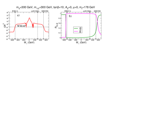
Figure 1: A plot of a) relic density $\Omega_{CDM}h^{2}$ and b) bino/wino component of the lightest neutralino as a function of $M_{1}$ for $m_{0}=300$ GeV, $m_{1/2}=300$ GeV, $A_{0}=0$, $\tan\beta=10$, $\mu>0$ and $m_{t}=178$ GeV.

In frame b), we show the amplitude, $R_{\widetilde{B},\widetilde{W}}$, for the bino/wino content of the lightest neutralino $\widetilde{Z}_{1}$. Here, we adopt the notation of Ref. [42, 38], wherein the lightest neutralino is written in terms of its (four component Majorana) Higgsino and gaugino components as

$$\widetilde{Z}_{1}=v_{1}^{(1)}\psi_{h_{u}^{0}}+v_{2}^{(1)}\psi_{h_{d}^{0}}+v_{3}^{(1)}\lambda_{3}+v_{4}^{(1)}\lambda_{0},$$ (6)

where $R_{\widetilde{W}}=|v_{3}^{(1)}|$ and $R_{\widetilde{B}}=|v_{4}^{(1)}|$. A striking difference between the positive and negative $M_{1}$ portions of frame b) is the shape of the level crossings at $R_{\widetilde{B}}=R_{\widetilde{W}}=1/\sqrt{2}$: while the transition from a bino-like to a wino-like LSP is gradual when $M_{1}>0$, it is much more abrupt for negative values of $M_{1}$. We had already anticipated this when we noted that for $M_{1}({\rm weak})=M_{2}({\rm weak})$ the mass eigenstates are the photino, and aside from a small admixture of higgsinos, the zino, while the corresponding eigenstates were bino-like and wino-like as long as $|M_{1}({\rm weak})-M_{2}({\rm weak})|$ was larger than the gaugino-higgsino mixing entries in the neutralino mass matrix. We also see that, for $M_{1}>0$, the MWDM scenario is realized for the value $M_{1}$ where $R_{\widetilde{W}}<\sin\theta_{W}\simeq 0.48$ as we also expected. Finally, again as we anticipated, for $M_{1}<0$, the BWCA scenario is obtained for $|M_{1}|$ just above the level crossing, when the LSP is mainly bino-like and close in mass to the wino-like $\widetilde{Z}_{1}$. For a bino-like LSP, annihilation to vector boson pairs is suppressed, and the only way to reduce the relic density in the case of large negative $M_{1}$ is by having rather small $\widetilde{Z}_{2}-\widetilde{Z}_{1}$ and $\widetilde{W}_{1}-\widetilde{Z}_{1}$ mass gaps, so that chargino and neutralino co-annihilation effects are large[43], and act to decrease the relic density. Of course, when $-M_{1}>M_{2}$, then the $\widetilde{Z}_{1}$ suddenly becomes pure wino-like, and very low relic density is obtained, as in the case of AMSB models.

Similar results are obtained by keeping $M_{1}=m_{1/2}$, and varying $M_{2}$, as shown in Fig. 2. The MWDM scenario is reached just to the right of the level crossing where $M_{2}({\rm weak})$ is slightly larger than $M_{1}({\rm weak})$, while the BWCA scenario is reached for $M_{2}=-156$ GeV, where $|M_{2}({\rm weak})|$ is again just above $|M_{1}({\rm weak})|$ and the $\widetilde{Z}_{1}$ is essentially a bino. Again, the $\widetilde{Z}_{2}-\widetilde{Z}_{1}$ and, as discussed just below, also the $\widetilde{W}_{1}-\widetilde{Z}_{1}$, mass gaps are very small, so that co-annihilation plays an essential role in reducing $\Omega_{\widetilde{Z}_{1}}h^{2}$ to an acceptable value. We see also that there is a region of mainly small negative $M_{2}$ values where $m_{\widetilde{W}_{1}}<m_{\widetilde{Z}_{1}}$, where a charged LSP is obtained. This is, of course, ruled out by the negative results for searches for charged stable relics from the Big Bang.

In both the MWDM and the BWCA scenarios, $\widetilde{Z}_{1},\ \widetilde{Z}_{2}$ and $\widetilde{W}_{1}$ are the lightest sparticles. They will likely have a large impact upon the phenomenology of these models. Of particular interest is the ordering of the mass spectrum of these particles. We work this out in the so-called large $|\mu|$ approximation, where $|\mu|\gg M_{1},M_{2}$ applicable in many models. The chargino sector, since it consists of just two states, is simple and $m_{\widetilde{W}_{1}}$ is given by a relatively simple and well known expression that we do not reproduce here (see e.g. Ref. [38]). The neutralino sector is much more complicated but, in the large $|\mu|$ approximation, it is possible to “integrate out” the higgsinos, and work with an effective low scale theory that only includes the neutral bino and wino as discussed in the Appendix. The couplings of winos and binos to higgsinos in the original theory manifests itself as a mixing between winos and binos in the effective theory, where this mixing is suppressed by $1/|\mu|$. To ${\cal O}(1/\mu^{2})$, the signed tree level neutralino masses are given (in terms of weak scale parameters) by,

$$(1+\frac{M_{W}^{2}}{\mu^{2}})m_{\widetilde{Z}_{1,2}}=\frac{M_{1}+M_{2}+a\sec^{2}\theta_{W}+M_{2}\eta\pm\kappa}{1(1+\eta)}+{\cal O}({1\over\mu^{3}})\;,$$ (7)

where

$$a={{M_{W}^{2}\sin 2\beta}\over\mu}\ll|M_{1}|,\ |M_{2}|,$$

$$\eta=\frac{M_{W}^{2}}{\mu^{2}}(-1+\tan^{2}\theta_{W})\ll 1,$$

and

$$\kappa^{2} = (M_{1}-M_{2})^{2}+2a(M_{1}+M_{2})\sec^{2}\theta_{W}+a^{2}\sec^{4}\theta_{W}$$

$$+ 2(M_{1}+M_{2})M_{2}\eta-4a(M_{1}+M_{2}\tan^{2}\theta_{W})-4M_{1}M_{2}\eta.$$

We emphasize that (7) is valid even when the gaugino masses are comparable to the gaugino-higgsino mixing terms in the neutralino mass matrix, and is a useful approximation as long as $|\mu|$ is large. If $M_{1}$ is not very close to $M_{2}$, we can simplify the expressions for $m_{\widetilde{Z}_{1,2}}$ by expanding $\kappa\simeq|M_{1}-M_{2}|$ plus terms that are suppressed by powers of $\mu$. Such an expansion then yields,

$$m_{\widetilde{Z}_{1}} = M_{1}+\frac{M_{W}^{2}}{\mu}\tan^{2}\theta_{W}\sin 2\beta-M_{1}\frac{M_{W}^{2}}{\mu^{2}}\frac{\sin^{2}2\beta\tan^{2}\theta_{W}}{M_{1}-M_{2}}+{\cal O}(1/\mu^{3}),$$

$$m_{\widetilde{Z}_{2}} = M_{2}+\frac{M_{W}^{2}}{\mu}\sin 2\beta-M_{2}\frac{M_{W}^{2}}{\mu^{2}}-\frac{M_{W}^{4}}{\mu^{2}}\frac{\tan^{2}\theta_{W}}{M_{1}-M_{2}}\sin^{2}2\beta+{\cal O}(1/\mu^{3}),$$ (8)

$$m_{\widetilde{W}_{1}} = M_{2}+\frac{M_{W}^{2}}{\mu}\sin 2\beta-\frac{M_{W}^{2}}{\mu^{2}}M_{2}+{\cal O}(1/\mu^{3})\;,$$

where we have assumed $|M_{1}|<|M_{2}|$ when we associated the bino-like state with $\widetilde{Z}_{1}$. Except for this, (8) are valid for all magnitudes and signs of $M_{1}$ and $M_{2}$, as long as $|M_{1}-M_{2}|\gg M_{W}^{2}/|\mu|$. In particular, we can use these expressions for the BWCA scenario, but for the MWDM case, we would have to use (7) to get the neutralino masses.

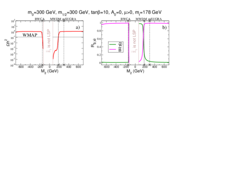
Figure 2: A plot of a) relic density $\Omega_{CDM}h^{2}$ and b) bino/wino component of the lightest neutralino as a function of $M_{2}$ for $m_{0}=300$ GeV, $m_{1/2}=300$ GeV, $A_{0}=0$, $\tan\beta=10$, $\mu>0$ and $m_{t}=178$ GeV.

The ordering of the mass spectrum of the lightest SUSY particles in the same sign MWDM and opposite sign BWCA scenarios is different, as can be seen from Fig. 3, where we plot the $\widetilde{W}_{1}$-$\widetilde{Z}_{2}$ mass splitting as a function of the absolute GUT-scale value $|M_{1}|/m_{1/2}$. For the MWDM case, the lightest chargino is lighter than the next-to-lightest neutralino, while the opposite holds true in the BWCA case. As long as $|M_{1}({\rm weak})|<|M_{2}({\rm weak})|$, both $\widetilde{W}_{1}$ and $\widetilde{Z}_{2}$ are dominantly wino-like, and the tree-level mass splitting between them can be read off from (8), as long as the weak scale values of $M_{1}$ and $M_{2}$ are not too close. We then find that at tree-level [44],

$$\Delta m_{\rm tree}\equiv m_{\widetilde{W}_{1}}-m_{\widetilde{Z}_{2}}\approx\frac{m_{W}^{4}\tan^{2}\theta_{W}}{(M_{1}({\rm weak})-M_{2}({\rm weak})\mu^{2})}\sin^{2}2\beta.$$ (9)

for all combinations of signs of gaugino masses. For the BWCA case, the denominator $|M_{1}({\rm weak})-M_{2}({\rm weak})|$ is very large, so that the tree level splitting is negligible compared to the one-loop splitting; the latter is always positive, hence in the opposite sign BWCA case, when the LSP is bino-like, the lightest chargino is always heavier than the next-to-lightest neutralino. In contrast, for the same-sign MWDM case, the tree level splitting (over the range of $M_{1}$ values where (9) is valid) is negative, and comparable to or larger than the one-loop splitting, so that the chargino is now usually heavier than $\widetilde{Z}_{2}$, as may be seen by the dashed line in Fig. 3.

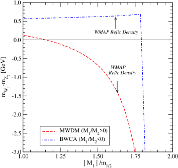
Figure 3: The mass splitting between the lightest chargino and the next-to-lightest neutralino, $m_{\widetilde{W}_{1}}-m_{\widetilde{Z}_{2}}$ in the BWCA scenario (dot-dashed blue line, with opposite $M_{1}$ and $M_{2}$ signs) and in the MWDM scenario (dashed red line, with same $M_{1}$ and $M_{2}$ signs), as a function of the absolute GUT scale value of $|M_{1}|/m_{1/2}$. The arrows indicate the value of $|M_{1}|/m_{1/2}$ where the neutralino thermal relic abundance equals the central WMAP CDM abundance value. The other SUSY parameters are as in Fig. 1.

Various other sparticle masses are also affected by varying the gaugino masses, since these feed into the soft term evolution via the RGEs. In Fig. 4, we show the variation of the sparticle mass spectrum with respect to the GUT scale ratio $M_{1}/m_{1/2}$ for the same parameters as in Fig. 1. In the mSUGRA case where $M_{1}/m_{1/2}=1$, there is a relatively large mass gap between $\widetilde{Z}_{2}$ and $\widetilde{Z}_{1}$: $m_{\widetilde{Z}_{2}}-m_{\widetilde{Z}_{1}}=106.7$ GeV. As $M_{1}$ varies to large positive values (the MWDM case), the mass gap shrinks to $m_{\widetilde{Z}_{2}}-m_{\widetilde{Z}_{1}}=31.9$ GeV. As $M_{1}$ varies to large negative values, the mass gap also decreases, this time to just 22.7 GeV in the BWCA scenario. We also note that as $|M_{1}|$ increases, the $\tilde{e}_{R}$, $\tilde{\mu}_{R}$ and $\tilde{\tau}_{1}$ masses also increase, since $M_{1}^{2}$ feeds into their mass evolution via RGEs. This also gives rise to the nearly symmetric behavior versus the sign of $M_{1}$ for the mass spectrum of first and second generation sfermions. As the coefficient appearing in front of $M_{1}$ in the RGEs is larger (and with the same sign) for the right handed sfermions than for the left handed ones, one expects, in general, a departure from the usual mSUGRA situation where the lightest sleptons are right-handed. As a matter of fact, whereas in mSUGRA $m_{\tilde{e}_{L}}>>m_{\tilde{e}_{R}}$ for $m_{0}\stackrel{{\scriptstyle<}}{{\sim}}m_{1/2}$, in the case of BWCA or MWDM, we find that $m_{\tilde{e}_{L}}\sim m_{\tilde{e}_{R}}$. As shown in the figure, the right-handed squark masses also increase with increasing $|M_{1}|$, although the relative effect is less dramatic than the case involving sleptons: the dominant driving term in the RGEs is, in this case, given by $M_{3}$ (absent in the case of sleptons), hence variations in the GUT value of $M_{1}$ produce milder effects. The trilinear SSB $A_{t},\ A_{b}$ and $A_{\tau}$ parameters have a linear dependence on gaugino mass in their RGEs, which means the weak scale $A$-parameters will be asymmetric versus the sign of $M_{1}$. The $\mu$ parameter is also slightly asymmetric. This gives rise to the asymmetric behavior of the third generaton sfermion masses with respect to the sign of the gaugino mass.

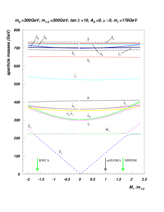
Figure 4: A plot of various sparticle masses vs. $M_{1}/m_{1/2}$ for $m_{0}=300$ GeV, $m_{1/2}=300$ GeV, $A_{0}=0$, $\tan\beta=10$ and $\mu>0$.

In Fig. 5, we show a plot of sparticle masses for the same parameters as in Fig. 4, but versus $M_{2}/m_{1/2}$. In this case, as $|M_{2}|$ is decreased from its mSUGRA value of 300 GeV, the $\widetilde{W}_{1}$ and $\widetilde{Z}_{2}$ masses decrease until $\Omega_{\widetilde{Z}_{1}}h^{2}$ reaches 0.11 in both the BWCA and MWDM scenarios. In this case, with decreasing $|M_{2}|$, the left- slepton and sneutrino masses also decrease, again leading to $m_{\tilde{e}_{L}}\sim m_{\tilde{e}_{R}}$. The left-handed squark masses similarly decrease. This increase is more pronounced that in Fig. 4 because the $SU(2)$ gauge coupling is larger than the $U(1)_{Y}$ gauge coupling. The $SU(2)$ singlet right-handed sfermion masses are not affected, with the net result that the mSUGRA $m_{\tilde{e}_{L}}>>m_{\tilde{e}_{R}}$ hierarchy is again altered.

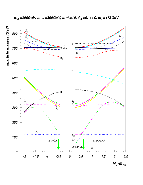
Figure 5: A plot of various sparticle masses vs. $M_{2}/m_{1/2}$ for $m_{0}=300$ GeV, $m_{1/2}=300$ GeV, $A_{0}=0$, $\tan\beta=10$ and $\mu>0$.

It should be apparent now that most points in the $m_{0}\ vs.\ m_{1/2}$ plane can become WMAP allowed by adopting an appropriate negative value of either $M_{1}$ or $M_{2}$ such that one enters into the BWCA scenario. The exception occurs if the WMAP-allowed point is obtained because the $A$-funnel or stau co-annihilation region is reached instead. To illustrate this, we plot in Fig. 6 the ratio $r_{1}\equiv M_{1}/m_{1/2}$ in frame a) or $r_{2}\equiv M_{2}/m_{1/2}$ in frame b) needed to achieve a relic density in accord with the WMAP central value. We see in frame a) that $r_{1}$ generally increases as one moves from lower-left to upper-right. The structure in the upper-left of the plot occurs when $-M_{1}$ is dialed to such a value that $2m_{\widetilde{Z}_{1}}\simeq m_{A}$, i.e. one is entering the $A$-funnel (even though $\tan\beta$ is relatively low) instead of the BWCA scenario. These regions will of course have a much larger $\widetilde{Z}_{2}-\widetilde{Z}_{1}$ mass gap than points in the BWCA scenario. Like the non-universal mass scenario [15], the BWCA scenario allows the $A$ funnel to be reached for any value of $\tan\beta$, but should be distinguishable from this because the $\widetilde{Z}_{1}-\widetilde{Z}_{2}$ mass gap, for instance, will be quite different in the two scenarios. In frame b), the ratio $r_{2}$ that gives rise to a WMAP-allowed point is shown to increase as one travels from lower to higher values of $m_{1/2}$. In this case, since the value of $M_{2}$ hardly changes the value of $m_{\widetilde{Z}_{1}}$, the $A$-funnel is never reached, and the BWCA region can be accessed over most of parameter space, save near the left-hand edge in the stau co-annihilation region.

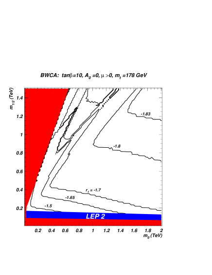
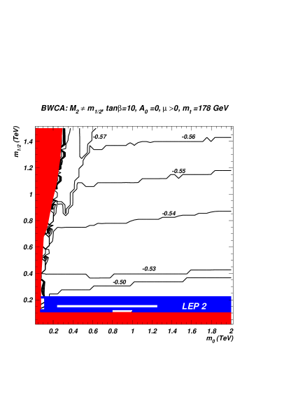
Figure 6: Contours of a) $r_{1}$ and b) $r_{2}$ in the $m_{0}\ vs.\ m_{1/2}$ plane for $\tan\beta=10$, $A_{0}=0$, $\mu>0$. Each point has $\Omega_{\widetilde{Z}_{1}}h^{2}=0.11$. The origin of the strips in the LEP excluded region of the right hand frame is discussed in Sec. 5.

3 Dark matter in the BWCA scenario

3.1 Neutralino relic density in the BWCA scenario: a closer look

In order to better understand the coannihilation mechanisms which drive the neutralino relic abundance within the WMAP preferred range in the BWCA vs. the MWDM scenario (with opposite and same signs for $M_{1}$ and $M_{2}$), we adopt the sample point defined by the mSUGRA input parameters ($m_{0}$=300 GeV, $m_{1/2}$=300 GeV, $\tan\beta$=10, sgn($\mu)>0$, $A_{0}$=0, $m_{\rm top}$=178 GeV), and pick the $M_{1}/m_{1/2}$ values which give $\Omega_{\widetilde{Z}_{1}}h^{2}=0.11$, i.e., respectively, $M_{1}/m_{1/2}=-1.619$ and $M_{1}/m_{1/2}=1.630$. We plot in Fig. 7 the thermally averaged cross section including coannihilations (solid) and without coannihilations (dashed lines) times the relative velocity as a function of the temperature $T$. In the same sign MWDM case, one notices that the very significant wino-component in the photino-like lightest neutralino gives a non-negligible $s$-wave contribution via annihilation to $W$ pairs, (i.e., a contribution which goes as $\langle\sigma v\rangle(T)\sim a$), while in the opposite sign BWCA case the lightest neutralino is a pure bino, and the squark mediated $t$-channel dominated pair annihilation cross section is strongly $s$-wave suppressed ($\langle\sigma v\rangle(T)\sim a^{\prime}+b^{\prime}(T/m_{\rm LSP})$, $a^{\prime}\ll b^{\prime}$). As a result, the pair annihilation cross section at $T=0$ (relevant for indirect DM detection) is more than one order of magnitude suppressed in the BWCA case.

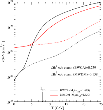
Figure 7: The thermally averaged effective pair annihilation cross section times velocity, $\langle\sigma v\rangle(T)$ as a function of the temperature, for the BWCA (black lines) and MWDM (red lines) scenarios. The dotted lines correspond to $\langle\sigma v\rangle(T)$ without the inclusion of coannihilation effects. The arrow indicates the approximate temperature where freeze-out occurs.

A second effect, also traced back to the lack of a significant wino component in the opposite sign BWCA case, is the role and onset of coannihilations. To isolate the role of coannihilations, we show by dashed lines $\langle\sigma v\rangle(T)$ computed without any coannihilation contribution. In the BWCA case, coannihilations play a much more important role, as can be understood by looking at the relative size of the cross sections with and without coannihilations around the lightest neutralino freeze-out temperature $T_{\rm f.o.}$, indicated by an arrow in the figure. Furthermore, in the BWCA case, the onset of the coannihilation regime takes place at lower temperatures, a reflection of the reduced mass splitting between the coannihilation partners and the LSP. At the freeze-out temperature, $\langle\sigma v\rangle(T)$ is dominated by coannihilations in the opposite sign BWCA case, while the relative coannihilation contribution for the MWDM case (for which the $\widetilde{Z}_{1}$s can annihilate to $WW$) is significantly smaller. Observe also the indicated relic abundance of the LSP computed without coannihilations, respectively 0.759 in the BWCA case and 0.138 in the same MWDM.

Coannihilations of particles $A$ and $B$ effectively enter the neutralino pair annihilation cross section when the center of mass momentum $p_{\rm c.m.}$ of the neutralino-neutralino system satisfies the relation

$$s=4p_{\rm c.m.}^{2}+4m_{\widetilde{Z}_{1}}^{2}\geq(m_{A}+m_{B})^{2}.$$ (10)

A suitable quantity to illustrate the onset of coannihilations is given by an effective annihilation rate $(\sigma v)_{\rm eff}$, defined as in Ref. [45]

$$(\sigma v)_{\rm eff}\equiv\frac{W_{\rm eff}(p_{\rm c.m.})}{4E^{2}_{\rm c.m.}},\qquad E_{\rm c.m.}=\sqrt{p_{\rm c.m.}^{2}+m_{\widetilde{Z}_{1}}^{2}}$$ (11)

(we refer the reader to Ref. [45] for the definition of the effective annihilation rate $W_{\rm eff}$, which is essentially the sum over all (co-)annihilation channels, properly weighted, of the various annihilation rates per unit volume and unit time) and such that

$$\lim_{p_{\rm c.m.}\rightarrow 0}(\sigma v)_{\rm eff}=\langle\sigma v\rangle(T=0).$$ (12)

The temperature dependence of $\langle\sigma v\rangle(T)$ is factored out in the weight function $\kappa(p_{\rm c.m.},T)$ [45], so that

$$\langle\sigma v\rangle(T)=\int_{0}^{\infty}{\rm d}p_{\rm c.m.}\frac{W_{\rm eff}(p_{\rm c.m.})}{4E^{2}_{\rm c.m.}}\kappa(p_{\rm c.m.},T).$$ (13)

In Fig. 8, we plot the two effective annihilation rates $(\sigma v)_{\rm eff}$ for the two BWCA and MWDM sample cases at the mSUGRA point given above, with the correct WMAP relic abundance. The coannihilation thresholds are shifted to larger $p_{\rm c.m.}$ values in the same sign case (the mass splitting of coannihilating partners is increased). The $\widetilde{W}_{1}$-$\widetilde{Z}_{2}$ mass splitting is too small to resolve the separate contributions, and the two bumps correspond to the onset of $\widetilde{Z}_{1}$-$\widetilde{W}_{1},\widetilde{Z}_{2}$ coannihilations and the onset of (co-)annihilations amongst $\widetilde{W}_{1}$ and $\widetilde{Z}_{2}$. When the bino-wino mixing is suppressed, the second processes contribute much more than the first processes to $(\sigma v)_{\rm eff}$. However, as shown by the weight function $\kappa(p_{\rm c.m.},T=T_{\rm f.o.})$, $(\sigma v)_{\rm eff}$ is largely sampled in a $p_{\rm c.m.}$ range where the $\widetilde{W}_{1},\widetilde{Z}_{2}$ (co-)annihilations are not kinematically accessible. This picture, however, depends on the LSP mass : had we picked a larger value for $m_{\widetilde{Z}_{1}}$, the mass splitting between $\widetilde{Z}_{1}$ and $\widetilde{Z}_{2},\ \widetilde{W}_{2}$ needed to obtain a sufficiently low relic abundance would have been smaller, so that the coannihilation bumps in $W_{eff}/4E^{2}$ would have occurred at smaller center-of-mass momenta, where the sampling function $\kappa$ has not yet fallen to very small values. In this case, the role of $\widetilde{W}_{1}-\widetilde{Z}_{2}$ coannihilations would have been enhanced even in the MWDM case.

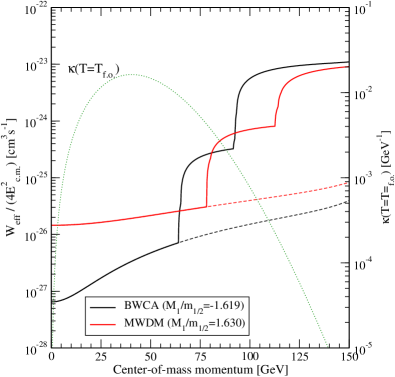
Figure 8: The effective $(\sigma v)_{\rm eff}$ term, as defined in Eq. (11), as a function of the center of mass momentum $p_{\rm eff}$, for the BWCA (black lines) and MWDM (red lines) scenarios, with (solid lines) and without (dotted lines) coannihilations. The green dotted line indicates the “weight function” $\kappa(p_{\rm c.m.},T=T_{\rm f.o.})$.

In the limit in which sfermions are heavy, and thus the bino annihilation cross section is extremely suppressed, and in which $\mu\gg M_{1}(\rm weak),\ M_{2}(\rm weak)$ (in the remainder of this paragraph, we will implicitly use $M_{1,2}=M_{1,2}(\rm weak)$), i.e., in the pure gaugino limit, the relic abundance should only depend on i.) the LSP mass scale and on ii.) the LSP-wino system splitting relative to the LSP mass. Since a pure wino-like system has a relic abundance which goes like [46]

$$\Omega_{\rm pure\ winos}h^{2}\simeq c\cdot\left(\frac{M_{2}}{1\ {\rm TeV}}\right)^{\gamma},\qquad c\simeq 0.024,\ \gamma\simeq 1.9,$$ (14)

the relic abundance of a coannihilating bino will be given by that of the pure wino system, rescaled by the exponential factor $\exp[-((M_{2}-M_{1})/M_{1})\cdot\widetilde{x})]$, with $\widetilde{x}\simeq M_{1}/T_{\rm f.o.}$, and rescaled by the new parasite bino degrees of freedom. The wino system carries 2+4 degrees of freedom, while the bino 2, hence we expect an enhancement of the relic abundance for a coannihilating bino of a factor $(4/3)^{2}$ [47]. The relic abundance should then take the form

$$\Omega_{\rm bino+wino}h^{2}\approx a\cdot\left(\frac{M_{2}}{1\ {\rm TeV}}\right)^{\gamma}\cdot\exp\left[\frac{M_{2}-M_{1}}{M_{1}}\cdot\widetilde{x}\right],\quad\quad a\approx c(4/3)^{2}.$$ (15)

Since $M_{2}\simeq M_{1}$, this allows in principle to define a strip in the $M_{1},\frac{M_{2}-M_{1}}{M_{1}}$ plane of WMAP preferred relic abundance. We show the result in Fig. 9, taking $\mu,m_{\widetilde{S}},m_{A}=100\cdot M_{2}$, $m_{\widetilde{S}}$ being all sfermion masses. Indeed, the iso-level curves for the relic abundance show the functional form of Eq. (15).

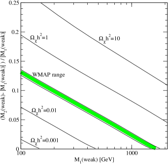
Figure 9: Iso-level curves at given values of the neutralino relic abundance in the $M_{1},(M_{2}-|M_{1}|)/|M_{1}|$ plane. The green strip indicates the WMAP 2-$\sigma$ range. We assumed here $\mu,m_{\widetilde{S}},m_{A}=100\cdot M_{2}$, $m_{\widetilde{S}}$ being all sfermion masses.

3.2 Direct and indirect detection of neutralino CDM

In this section, we turn to consequences of the BWCA scenario for direct and indirect detection of neutralino dark matter[48]. We adopt the DarkSUSY code[49], interfaced to Isajet, for the computation of the various rates, and resort to the Adiabatically Contracted N03 Halo model[50] for the dark matter distribution in the Milky Way. We evaluate the following neutralino DM detection rates:

• Direct neutralino detection via underground cryogenic detectors[54]. Here, we compute the spin independent neutralino-proton scattering cross section, and compare it to expected sensitivities[55] for Stage 2 detectors (CDMS2[56], Edelweiss2[57], CRESST2[58], ZEPLIN2[59]) and for Stage 3, ton-size detectors (XENON[60], GERDA[61], ZEPLIN4[62] and WARP[63]). We take here as benchmark experimental reaches of Stage 2 and Stage 3 detectors the projected sensitivities of, respectively, CDMS2 and XENON 1-ton at the corresponding neutralino mass.

• Indirect detection of neutralinos via neutralino annihilation to neutrinos in the core of the Sun[64]. Here, we present rates for detection of $\nu_{\mu}\rightarrow\mu$ conversions at Antares[65] or IceCube[66]. The reference experimental sensitivity we use is that of IceCube, with a muon energy threshold of 25 GeV, corresponding to a flux of about 40 muons per ${\rm km}^{2}$ per year.

• Indirect detection of neutralinos via neutralino annihilations in the galactic center leading to gamma rays[67], as searched for by EGRET[68], and in the future by GLAST[69]. We evaluate the integrated continuum $\gamma$ ray flux above a $E_{\gamma}=1$ GeV threshold, and assume a GLAST sensitivity of 1.0$\times 10^{-10}\ {\rm cm}^{-2}{\rm s}^{-1}$.

• Indirect detection of neutralinos via neutralino annihilations in the galactic halo leading to cosmic antiparticles, including positrons[70] (HEAT[71], Pamela[72] and AMS-02[73]), antiprotons[74] (BESS[75], Pamela, AMS-02) and anti-deuterons ($\bar{D}$s) (BESS[76], AMS-02, GAPS[77]). For positrons and antiprotons we evaluate the averaged differential antiparticle flux in a projected energy bin centered at a kinetic energy of 20 GeV, where we expect an optimal statistics and signal-to-background ratio at space-borne antiparticle detectors[53, 78]. We take the experimental sensitivity that of the Pamela experiment after three years of data-taking as our benchmark. Finally, the average differential antideuteron flux has been computed in the $0.1<T_{\bar{D}}<0.4$ GeV range, where $T_{\bar{D}}$ stands for the antideuteron kinetic energy per nucleon, and compared to the estimated GAPS sensitivity[77] (see Ref. [79] for an updated discussion of the role of antideuteron searches in DM indirect detection).

In Fig. 10, we show various direct and indirect DM detection rates for $m_{0}=m_{1/2}=300$ GeV, with $A_{0}=0$, $\tan\beta=10$ and $\mu>0$, while $M_{1}$ is allowed to vary. The $M_{1}$ value corresponding to the mSUGRA model is denoted by a dot-dashed vertical line, while the BWCA and MWDM scenarios with $\Omega_{\widetilde{Z}_{1}}h^{2}=0.11$ are denoted by dash-dash-dot and dashed vertical lines, respectively. The dotted lines correspond to the sensitivity level of each of these experiments; i.e., the signal is observable only when the model prediction is higher than the corresponding dotted line. While the minimum sensitivity for the direct detection rates in frames b) – f) refers to the minimum magnitude of the signal that is detectable (and hence independent of the LSP mass), the smallest detectable cross section shown by the dotted curves in frame a) depends on the value of $m_{\widetilde{Z}_{1}}$.

In frame a), we plot the spin-independent neutralino-proton scattering cross section. We see that as $M_{1}$ is decreased, and becomes increasingly negative, the neutralino-proton scattering cross section plummets to values in the $10^{-12}$ pb range, far below the sensitivity of any planned detector. The drop-off is due to increasing negative interference amongst the contributing Feynman diagrams.

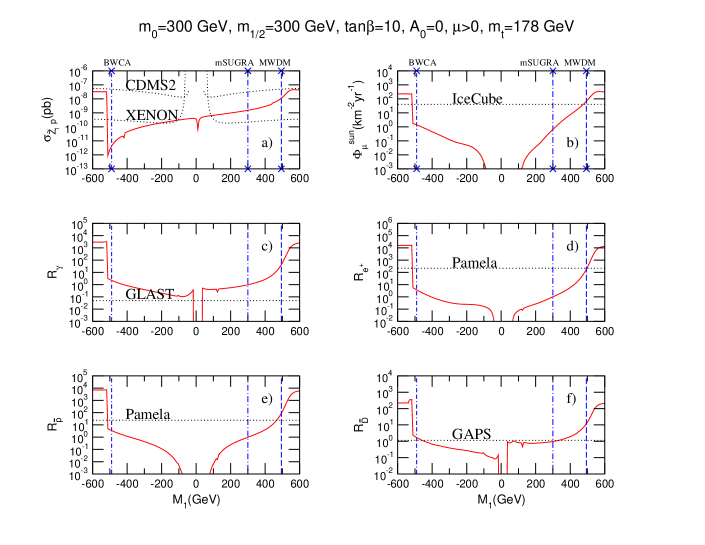
Figure 10: Rates for direct and indirect detection of neutralino dark matter vs. $M_{1}$ for $m_{0}=m_{1/2}=300$ GeV, with $\tan\beta=10$, $A_{0}=0$, $\mu>0$. Frames c) -f) show the ratio of indirect detection rates compared to the mSUGRA model. In this plot, we adopt the adiabatically contracted N03 distribution for halo dark matter.

In frame b), we show the flux of muons from neutralino pair annihilations in the core of the Sun. The muon flux is below the reach of IceCube in the mSUGRA case, and it remains below IceCube observability in the BWCA case. The rate for neutralino annihilation in the sun or earth is given by

$$\Gamma_{A}={1\over 2}C\tanh^{2}(t_{\odot}/\tau),$$ (16)

where $C$ is the capture rate, $A$ is the total annihilation rate times relative velocity per volume, $t_{\odot}$ is the present age of the solar system and $\tau=1/\sqrt{CA}$ is the equilibration time. For small $C$, as shown in frame a), the equilibration time becomes large, so that $\Gamma_{A}\sim\frac{1}{2}C^{2}At^{2}$, and is hence sensitive to the neutralino annihilation cross section times relative velocity, unlike cases where the neutralino-nucleon scattering cross section is large. The muon flux jumps to observable levels at more negative values of $M_{1}$, but this is only because the $\widetilde{Z}_{1}$ suddenly becomes wino-like, so that the relic density becomes too low.

In frames c), d), e) and f) we show the flux of photons, positrons, antiprotons and antideuterons, respectively. The results here are plotted as ratios of fluxes normalized to the mSUGRA point, in order to give results that are approximately halo-model independent. (We do show the above described expected experimental reach lines as obtained by using the Adiabatically Contracted N03 Halo model[50].) The rates for indirect detection via observation of halo annihilation remnants are typically low in the BWCA scenario, since the bino annihilation cross sections are $s$-wave suppressed. Observable results are indicated for $\gamma$ rays by GLAST, but this is due in part to the very favorable N03 halo distribution which is assumed.

In Fig. 11, we show the same direct and indirect DM detection rates as in Fig. 10, except this time versus $M_{2}$ instead of $M_{1}$. In frame a), the neutralino-nucleon scattering rates do not have negative interference, and can remain at observable, although not enhanced, levels. The rates for detection of BWCA DM at IceCube are relatively low, as are rates for anti-matter detection by Pamela in frames d) and e). The rates for $\gamma$ detection by GLAST in frame c) are similar to those from the mSUGRA case, while the rate for antideuteron detection by GAPS is just barely observable for BWCA DM in frame f).

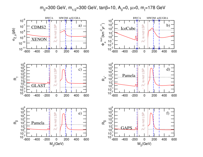
Figure 11: Rates for direct and indirect detection of neutralino dark matter vs. $M_{2}$ for $m_{0}=m_{1/2}=300$ GeV, with $\tan\beta=10$, $A_{0}=0$, $\mu>0$. Frames c) -f) show the ratio of indirect detection rates compared to the mSUGRA model. In this plot, we adopt the adiabatically contracted N03 distribution for halo dark matter.

Overall, prospects for direct or indirect detection of BWCA dark matter are generally at or below levels expected in the mSUGRA model. For this reason, we do not present direct and indirect detection rates in the $m_{0}\ vs.\ m_{1/2}$ plane. We also mention that the situation is sharply different in the MWDM scenarios where the corresponding rates are generally larger than in the mSUGRA model. Thus, a detection of a signal in the XENON or Pamela experiments could serve to discriminate between these scenarios, especially if we already have some information of the SUSY spectrum from collider experiments.

4 Neutralino radiative decay in the BWCA scenario

The loop-induced radiative decay width for $\widetilde{Z}_{2}\rightarrow\widetilde{Z}_{1}\gamma$ has been calculated in Ref. [80, 81]. A thorough numerical analysis[82, 83] has shown that the radiative decay can be large and even dominant in certain regions of MSSM parameter space. A necessary (but not sufficient) condition for this is that all tree level two body decay modes of $\widetilde{Z}_{2}$ be kinematically forbidden. In this case, $\widetilde{Z}_{2}$ usually decays via $\widetilde{Z}_{2}\rightarrow\widetilde{Z}_{1}f{\bar{f}}$, where $f$ is a light SM fermion. However, if $\widetilde{Z}_{1}$ and $\widetilde{Z}_{2}$ are close in mass, the formally higher order two body radiative decay becomes competitive with the three body decays $\widetilde{Z}_{2}\rightarrow f\bar{f}\widetilde{Z}_{1}$. This is because $\Gamma(\widetilde{Z}_{2}\rightarrow\widetilde{Z}_{1}\gamma)\propto(1-m_{\widetilde{Z}_{1}}/m_{\widetilde{Z}_{2}})^{3}$, while $\Gamma(\widetilde{Z}_{2}\rightarrow\widetilde{Z}_{1}f\bar{f})\propto(1-m_{\widetilde{Z}_{1}}/m_{\widetilde{Z}_{2}})^{5}$.

As we have seen, in both the MWDM and BWCA scenarios $m_{\widetilde{Z}_{2}}-m_{\widetilde{Z}_{1}}$ is small, so that we may expect that the branching fraction for radiative decays may be enhanced. Moreover, in both cases, the couplings of the neutralinos to the $Z$ boson, which occur only via the higgsino components of the neutralino are strongly suppressed so that virtual $Z$ boson exchange contribution to three body decay amplitudes is correspondingly suppressed. However, vector boson-gaugino loops essentially also decouple from the radiative decay in the BWCA case because the bino does not couple to these. These do not, however, decouple in the MWDM case since both the photino and the zino couple to $W^{\pm}\widetilde{W}^{\mp}$ system. The branching fraction for the radiative decay is thus a result of a complicated interplay between the kinematic and dynamic effects discussed above.

In Fig. 12, we show in upper frame a) the neutralino relic density, and in b) the $BF(\widetilde{Z}_{2}\rightarrow\widetilde{Z}_{1}\gamma)$ for the same parameters as in Fig. 1, versus GUT scale gaugino mass $M_{1}$. The radiative branching fraction at this point in the mSUGRA model is just $\sim 10^{-5}$. As $M_{1}$ climbs to 490 GeV, in the MWDM case, the branching fraction has climbed to $\sim 5\%$. When $M_{1}$ varies to large negative values in the BWCA case, the branching fraction has climbed to $10\%$. In this case, we may expect that a considerable fraction of SUSY events at colliders to contain hard isolated photons via the decay of $\widetilde{Z}_{2}$ that is produced either directly, or via cascade decays of heavier sparticles. In the two lower frames, we show the same figures except for large $m_{0}=1$ TeV. In this case, the sfermion loops mediating the $\widetilde{Z}_{2}\rightarrow\widetilde{Z}_{1}\gamma$ decay become suppressed, and the branching fraction is much smaller, reaching $\sim 8\%$ in the MWDM case, and just $1\%$ in the BWCA case.

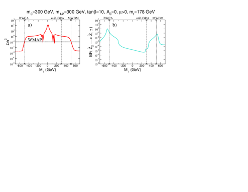
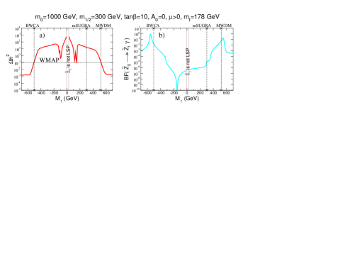
Figure 12: Upper: A plot of a) relic density $\Omega_{CDM}h^{2}$ and b) $BF(\widetilde{Z}_{2}\rightarrow\widetilde{Z}_{1}\gamma$) as a function of $M_{1}$ for $m_{0}=300$ GeV, $m_{1/2}=300$ GeV, $A_{0}=0$, $\tan\beta=10$, $\mu>0$ and $m_{t}=178$ GeV. Lower: Same plot for $m_{0}=1000$ GeV.

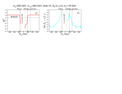
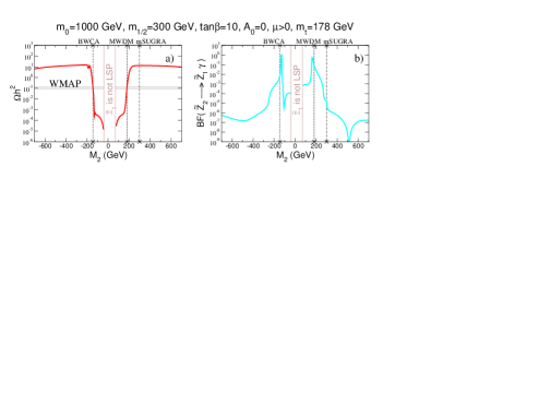
Figure 13: Upper: A plot of a) relic density $\Omega_{CDM}h^{2}$ and b) $BF(\widetilde{Z}_{2}\rightarrow\widetilde{Z}_{1}\gamma$) as a function of $M_{2}$ for $m_{0}=300$ GeV, $m_{1/2}=300$ GeV, $A_{0}=0$, $\tan\beta=10$, $\mu>0$ and $m_{t}=178$ GeV. Lower: Same plot for $m_{0}=1000$ GeV.

A similar situation is illustrated in Fig. 13, where now we plot versus variable $M_{2}$, while keeping $M_{1}=m_{1/2}=300$ GeV. In the upper frames for $m_{0}=300$ GeV, we see that while $BF(\widetilde{Z}_{2}\rightarrow\widetilde{Z}_{1}\gamma)$ reaches $5\%$ in the MWDM case, it reaches 25% in the BWCA scenario. In the lower frames, we see that for $m_{0}=1$ TeV, the branching fraction reaches $8\%$ for the case of MWDM and 0.8% for BWCA dark matter. We note that in both figures $B(\widetilde{Z}_{2}\rightarrow\widetilde{Z}_{1}\gamma)$ attains a higher value at its peak when $M_{1}/M_{2}$ is negative because it is in this case that the sparticle masses get really close (see the level crossings in Figs. 4 and 5).

,
,

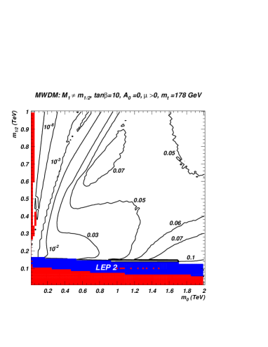
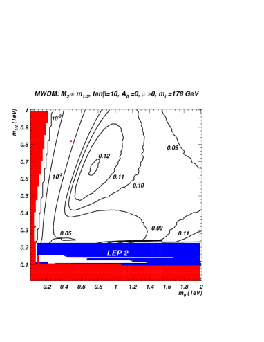
Figure 14: Contours of $BF(\widetilde{Z}_{2}\rightarrow\widetilde{Z}_{1}\gamma)$ in the $m_{0}\ vs.\ m_{1/2}$ plane for $\tan\beta=10$, $A_{0}=0$, $\mu>0$, $m_{t}=178$ GeV. In a)., we have adjusted $M_{1}$ everywhere to negative values so that $\Omega_{\widetilde{Z}_{1}}h^{2}=0.11$ in the BWCA scenario. In b)., we have adjusted $M_{2}$ everywhere to negative values so that $\Omega_{\widetilde{Z}_{1}}h^{2}=0.11$ in the BWCA scenario. In c). (d).), we have adjusted $M_{1}$ and ($M_{2}$) everywhere to positive values so that $\Omega_{\widetilde{Z}_{1}}h^{2}=0.11$ in the MWDM scenario.

In Fig. 14, we plot contours of $BF(\widetilde{Z}_{2}\rightarrow\widetilde{Z}_{1}\gamma)$ in the $m_{0}\ vs.\ m_{1/2}$ plane for $A_{0}=0$, $\tan\beta=10$, $\mu>0$ and $m_{t}=178$ GeV. At every point in the plane of frame a), we have adjusted $M_{1}$ to a negative value chosen so that $\Omega_{\widetilde{Z}_{1}}h^{2}=0.11$ in the BWCA scenario. We see that the $BF(\widetilde{Z}_{2}\rightarrow\widetilde{Z}_{1}\gamma)$ exceeds 50% around $m_{0}\sim 600-1000$ GeV for $m_{1/2}\sim 1-1.4$ TeV. The branching fraction remains large at all $m_{1/2}$ values, but diminishes for $m_{0}\stackrel{{\scriptstyle>}}{{\sim}}500-1000$ GeV. In Fig. 14b), we plot the same contours except that at every point in the plane, we have instead adjusted $M_{2}$ to negative values so that $\Omega_{\widetilde{Z}_{1}}h^{2}=0.11$. In this case, we see again that the branching fraction can become larger than 0.3 for low $m_{0}$ values. In frames c) and d) once again we show contours of $B(\widetilde{Z}_{2}\rightarrow\widetilde{Z}_{1}\gamma)$ but for the case of MWDM, where $M_{1}$ and $M_{2}$ are dialed to positive values. While the radiative branching fractions never reach much beyond the 10% level for MWDM, they maintain a significant rate out to large values of $m_{0}$. This is because in the MWDM case the radiative loop decays are dominated by $W$-chargino exchange, whereas in the BWCA case the radiative loops are dominated by fermion-sfermion exchange.

5 BWCA dark matter at colliders

5.1 $\widetilde{Z}_{2}-\widetilde{Z}_{1}$ mass gap in BWCA scenario

An important question is whether collider experiments would be able to distinguish the case of BWCA dark matter from other forms of neutralino DM such as MHDM as occur in the mSUGRA model or MWDM. We have seen from the plots of sparticle mass spectra that the squark and gluino masses vary only slightly with changing $M_{1}$ or $M_{2}$. However, the chargino and neutralino masses change considerably, and in fact rather small mass gaps $m_{\widetilde{W}_{1}}-m_{\widetilde{Z}_{1}}$ and $m_{\widetilde{Z}_{2}}-m_{\widetilde{Z}_{1}}$ are in general expected in both BWCA and MWDM scenarios, as compared to the case of models that incorporate gaugino mass unification close to the GUT scale.

In Fig. 15, we show contours of the mass gap $m_{\widetilde{Z}_{2}}-m_{\widetilde{Z}_{1}}$ in the $m_{0}\ vs.\ m_{1/2}$ plane for $A_{0}=0$, $\tan\beta=10$ and $\mu>0$ for a) the mSUGRA model, b) the case of BWCA DM where $-M_{1}$ is raised at every point until $\Omega_{\widetilde{Z}_{1}}h^{2}\rightarrow 0.11$ and c) the case of BWCA DM where $-M_{2}$ is lowered until $\Omega_{\widetilde{Z}_{1}}h^{2}\rightarrow 0.11$. In the case of the mSUGRA model, most of the parameter space has $m_{\widetilde{Z}_{2}}-m_{\widetilde{Z}_{1}}>90$ GeV, which means that $\widetilde{Z}_{2}\rightarrow\widetilde{Z}_{1}Z^{0}$ decay is allowed. When this decay is allowed, its branching fraction is always large, unless it competes with other two-body decays such as $\widetilde{Z}_{2}\rightarrow\widetilde{Z}_{1}h$ or $\widetilde{Z}_{2}\rightarrow\bar{f}\tilde{f}$ or $f{\bar{\tilde{f}}}$ (where $f$ is a SM fermion). In the case of BWCA DM in frames b) and c), we see that (aside from the left-most portion of frame b), which is not a region of BWCA), the mass gap is much smaller, so that two-body tree level decays of $\widetilde{Z}_{2}$ and $\widetilde{W}_{1}$ are closed and three-body decays are dominant. If $\widetilde{Z}_{2}$’s are produced at large rates either directly or via gluino or squark cascade decays[84], it should be possible to identify opposite sign/ same flavor dilepton pairs from their decays, to reconstruct their invariant mass, and extract the upper edge of the invariant mass distribution[85, 86].

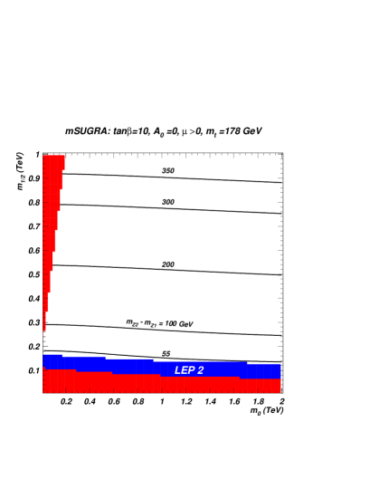
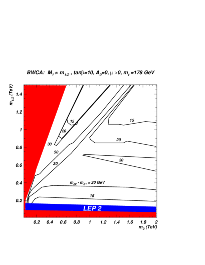
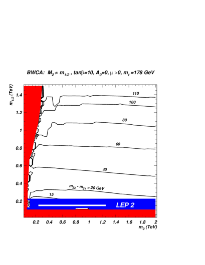
Figure 15: Contours of $m_{\widetilde{Z}_{2}}-m_{\widetilde{Z}_{1}}$ mass gap in the $m_{0}\ vs.\ m_{1/2}$ plane for $\tan\beta=10$, $A_{0}=0$, $\mu>0$ and a) mSUGRA model, b) $-M_{1}>m_{1/2}$ BWCA and c) $-M_{2}<m_{1/2}$ BWCA.

Finally, we note one curious feature of Fig. 15c that was referred to in the caption of Fig. 6. Within the blue shaded LEP2 excluded region there appear three allowed strips. The lower horizontal strip at $m_{1/2}\sim 100$ GeV corresponds to the neutralino $Z$-annihilation funnel, where $M_{2}$ does not have to be dialed to low values, since $Z$ annihilation already reduces the relic density. However, in this case where $M_{2}$ is negative, terms in the two-loop gaugino mass RGE conspire to yield a weak scale $|M_{2}|$ value which is somewhat larger than its mSUGRA counterpart. This means that while $2m_{\widetilde{Z}_{1}}\sim M_{Z}$, at the same time $m_{\widetilde{W}_{1}}$ is just above $103.5$ GeV, and is thus LEP2 allowed. A similar situation occurs for the longer allowed strip at $m_{1/2}\sim 150$ GeV, except in this case it is the $h$ resonance which reduces the relic density. Finally, at very low $m_{0}\sim 80$ GeV, bulk annihilation via light sleptons reduces the relic density, while the negative $M_{2}$ pushed $m_{\widetilde{W}_{1}}$ above the LEP2 limit. The corresponding strips do not appear in frame b) because here, we have only scanned $M_{1}$ values above $m_{1/2}$, as required to get agreement with WMAP: as we can see from Fig. 1 that the $Z$ and $h$ resonances appear for $|M_{1}|<m_{1/2}$.

5.2 Fermilab Tevatron

In the mSUGRA model, the best reach for SUSY at the Fermilab Tevatron occurs in the clean trilepton channel[87, 88]. We examined the clean trilepton signal rate for case study point BWCA3. For this point, the total SUSY particle production cross section was $\sim 440$ fb for $\sqrt{s}=2$ TeV $p\bar{p}$ collisions. Using the soft trilepton cuts SC2 of Ref. [88] (three isolated leptons with $p_{T}(\ell_{1},\ell_{2},\ell_{3})>11,7,5$ GeV, $|\eta(\ell_{1,2/3})|<1,2$, $E_{T}^{\rm miss}>25$ GeV, $m(\ell\bar{\ell})>20$ GeV, $m_{T}(\ell,E_{T}^{\rm miss})<60$ GeV plus a $Z$ mass veto), we find a surviving signal cross section of only 0.035 fb, well below observability. The main problem here is the $m(\ell\bar{\ell})>20$ GeV cut. This cut is essential to remove background from virtual photons in $q\bar{q}^{\prime}\rightarrow\ell\nu_{\ell}\ell^{\prime}\bar{\ell}^{\prime}$ electroweak production. However, the cut also kills much of the SUSY signal in the BWCA case, since the $\ell\bar{\ell}$ invariant mass is constrained to be $<m_{\widetilde{Z}_{2}}-m_{\widetilde{Z}_{1}}$, which is already quite small.

Another possibility is to search for events at the Tevatron containing isolated high $E_{T}$ photons from radiative $\widetilde{Z}_{2}$ decays. We examined the isolated photon inclusive channel ($E_{T}(\gamma)>8$ GeV with $\sum_{cone}^{R=0.4}E_{T}<0.1E_{T}(\gamma)$ and $|\eta(\gamma)|<1.1$), the photon plus lepton channel ($p_{T}(\ell)>15$ GeV with $\sum_{cone}^{R=0.4}E_{T}<5$ GeV and $E_{T}^{\rm miss}>20$ GeV), and photon plus $E_{T}^{\rm miss}>20$ GeV channels for the BWCA3 case study (see Table 2). In the latter two channels, we also vetoed jets. The signal rates were 43, 2.7 and 13.5 fb respectively, while backgrounds from $W\gamma$ ($Z\gamma$) production were 6911 (1803), 2500 (6.2) and 394 (253) fb, respectively. In light of these results, it appears very difficult to use the isolated photon channels in the BWCA scenario to identify SUSY at the Tevatron.

5.3 CERN LHC

If the $R$-parity conserving MSSM is a good description of nature at the weak scale, then multi-jet plus multi-lepton plus $E_{T}^{\rm miss}$ events should occur at large rates at the CERN LHC, provided that $m_{\tilde{g}}\stackrel{{\scriptstyle<}}{{\sim}}2-3$ TeV[89]. The LHC reach for SUSY in the mSUGRA model has been calculated in Ref. [90, 91]. The ultimate mSUGRA reach results, coming from the $E_{T}^{\rm miss}+$ jets channel, should also apply qualitatively to the BWCA case, since the values of $m_{\tilde{g}}$ and $m_{\tilde{q}}$ change little in going from mSUGRA to BWCA, and the $E_{T}^{\rm miss}+$ jets reach mainly depend on these masses.

The reach in other channels such as multileptons plus jets and isolated photons plus jets may change substantially in the BWCA scenario. The reach of the LHC in the ($m_{0},\ m_{1/2}$) plane of the mSUGRA model was recently re-assessed in Ref. [91] . The search strategy was based on the detection of gluino and squark cascade decay products, namely multiple high transverse momentum jets and/or leptons and/or photons plus large missing transverse energy. Here, we use Isajet 7.72^′ [39] for the simulation of signal and background events at the LHC. The event and detector simulation was performed along the lines established in Ref. [91], where details on cuts and detector resolution along with our definitions of jets and isolated leptons and photons may be found.

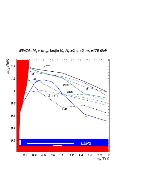
Figure 16: Reach contours of the CERN LHC for 100 fb^-1 of integrated luminosity for various signal topologies in the $m_{0}\ vs.\ m_{1/2}$ plane for $\tan\beta=10$, $A_{0}=0$, $\mu>0$ and for $-M_{2}<m_{1/2}$ such that $\Omega_{\widetilde{Z}_{1}}h^{2}=0.11$ at every point in the plane.

We plot the reach of the LHC in Fig. 16 for the BWCA case using the procedure described in [91]. All events had to pass the pre-cuts, which impose the requirement that $E_{T}^{\rm miss}>200$ GeV and there are at least 2 jets with $p_{T}^{\rm jet}>40$ GeV. We then optimized the cuts using the strategy in Ref. [91] – generally speaking, harder jet $E_{T}$ and $E_{T}^{\rm miss}$ cuts apply for heavier sparticles, and softer cuts apply for lighter sparticles. The events are divided into several classes, characterized by the number of leptons or the presence of an isolated photon in the final state. The $5\sigma$ discovery reach for 100 $fb^{-1}$ of integrated luminosity is shown for the various channels. The ultimate reach in the $E_{T}^{\rm miss}+$ jets channel ranges from $m_{1/2}\sim 1.4$ TeV at low $m_{0}$ to $m_{1/2}\sim 1$ TeV at $m_{0}=2$ TeV. These results are similar to those obtained in the mSUGRA model. The reach contour in the isolated photon plus jets plus $E_{T}^{\rm miss}$ channel, however, has greatly increased in the BWCA scenario compared to the mSUGRA case. In mSUGRA, the reach contour varies from $m_{1/2}:850\rightarrow 500$ GeV as $m_{0}:.1\rightarrow 2$ TeV. In the BWCA case, where $\widetilde{Z}_{2}\rightarrow\widetilde{Z}_{1}\gamma$ at a large rate, the photon reach contour reaches a maximum of $m_{1/2}=1.2$ TeV for $m_{0}\sim 500$ GeV. Thus, at CERN LHC, the BWCA scenario will be signalled by multijet plus isolated multilepton plus $E_{T}^{\rm miss}$ events, but with a large content of hard isolated photons as well, at least for the case where $m_{0}\stackrel{{\scriptstyle<}}{{\sim}}1$ TeV. For larger values of $m_{0}>1$ TeV, the $\widetilde{Z}_{2}\rightarrow\widetilde{Z}_{1}\gamma$ branching fraction drops, and the reach projections become similar to the case of mSUGRA. We have also checked that the reach using the $\gamma+n$ lepton channel is smaller than the reach via the corresponding $n$ lepton channel, primarily because the signal becomes too small to pass our 10 event/100 fb^-1 requirement.

For SUSY searches at the CERN LHC, Hinchliffe et al. have pointed out[86] that an approximate value of $m_{\tilde{q}}$ or $m_{\tilde{g}}$ can be gained by extracting the maximum in the $M_{eff}$ distribution, where $M_{eff}=E_{T}^{\rm miss}+E_{T}(jet\ 1)+E_{T}(jet\ 2)+E_{T}(jet\ 3)+E_{T}(jet\ 4)$. Their analysis will carry over to the BWCA scenario, as well as in models with gaugino mass unification, so that the approximate mass scale of strongly interacting sparticles will be known soon after a supersymmetry signal has been established.

In mSUGRA, a dilepton mass edge should be visible in SUSY signal events only if $m_{1/2}\stackrel{{\scriptstyle<}}{{\sim}}250$ GeV or if $\widetilde{Z}_{2}\rightarrow\tilde{\ell}\bar{\ell},\ \bar{\tilde{\ell}}\ell$ decays are allowed. In the case of BWCA DM, as with MWDM, the dilepton mass edge should be visible over almost all parameter space. We illustrate the situation for four case studies listed in Table 2. The first case, labeled mSUGRA, has $m_{0}=m_{1/2}=300$ GeV, with $A_{0}=0$, $\tan\beta=10$ and $\mu>0$. In this case, $\tilde{g}\tilde{g}$, $\tilde{g}\tilde{q}$ and $\tilde{q}\tilde{q}$ production occurs with a combined cross section of about 12 pb, while the total SUSY cross section is around 13.4 pb (the additional 1.4 pb comes mainly from -ino pair production and -ino-squark or -ino-gluino associated production). The case of BWCA1, with $M_{1}=-480$ GeV, has similar rates of sparticle pair production. The case of BWCA2, with lighter chargino and neutralino masses, has a total production cross section of 19.2 pb, wherein strongly interacting sparticles are pair produced at similar rates as in mSUGRA or BWCA1, but -ino pairs are produced at a much larger rate $\sim 6.1$ pb. We also show the case of BWCA3, which is similar to that of BWCA2 except that $\mu<0$, which gives a better fit to $(g-2)_{\mu}$ measurements.

parameter	mSUGRA	BWCA1	BWCA2	BWCA3
$M_{1}$	300	-480	300	300
$M_{2}$	300	300	-156	-170
$\mu$	409.2	401.3	402.3	-401.6
$m_{\tilde{g}}$	732.1	733.4	736.3	736.8
$m_{\tilde{u}_{L}}$	713.9	715.3	701.9	703.5
$m_{\tilde{t}_{1}}$	523.4	535.0	554.8	566.4
$m_{\tilde{b}_{1}}$	650.0	651.8	645.1	646.1
$m_{\tilde{e}_{L}}$	364.7	371.6	324.5	327.7
$m_{\tilde{e}_{R}}$	322.8	352.7	322.6	322.6
$m_{\widetilde{W}_{2}}$	432.9	426.0	419.6	421.3
$m_{\widetilde{W}_{1}}$	223.9	223.4	138.5	141.7
$m_{\widetilde{Z}_{4}}$	433.7	425.0	415.2	419.7
$m_{\widetilde{Z}_{3}}$	414.8	409.4	414.0	410.0
$m_{\widetilde{Z}_{2}}$	223.7	222.7	138.6	141.4
$m_{\widetilde{Z}_{1}}$	117.0	200.0	116.8	118.8
$m_{A}$	538.7	537.1	508.4	508.5
$m_{H^{+}}$	548.0	546.4	517.9	518.0
$m_{h}$	115.7	115.3	114.0	112.7
$\Omega_{\widetilde{Z}_{1}}h^{2}$	1.1	0.11	0.10	0.12
$BF(b\rightarrow s\gamma)$	$3.2\times 10^{-4}$	$3.3\times 10^{-4}$	$3.7\times 10^{-4}$	$4.6\times 10^{-4}$
$\Delta a_{\mu}$	$12.1\times 10^{-10}$	$9.9\times 10^{-10}$	$-13.8\times 10^{-10}$	$13.1\times 10^{-10}$
$\sigma_{sc}(\widetilde{Z}_{1}p)$	$1.5\times 10^{-9}\ {\rm pb}$	$4.7\times 10^{-12}\ {\rm pb}$	$1.2\times 10^{-9}\ {\rm pb}$	$8.0\times 10^{-11}\ {\rm pb}$
$BF(\widetilde{Z}_{2}\rightarrow\widetilde{Z}_{1}\gamma)$	$2.7\times 10^{-5}$	0.096	0.25	0.25

Table 2: Masses and parameters in GeV units for mSUGRA and three BWCA scenarios. In each case, $m_{0}=m_{1/2}=300$ GeV, $A_{0}=0$, $\tan\beta=10$ and $m_{t}=178$ GeV. The third BWCA case has $\mu<0$, while the first two have $\mu>0$.

We have generated 50K LHC SUSY events for each of these cases using Isajet 7.72^′, and passed them through a toy detector simulation as described above. Since gluino and squark masses of the three case studies are similar to those of LHC point 5 of the study of Hinchliffe et al.[86], we adopt the same overall signal selection cuts which efficiently select the SUSY signal while essentially eliminating SM backgrounds: $E_{T}^{\rm miss}>max(100\ {\rm GeV},0.2M_{eff})$, at least four jets with $E_{T}>50$ GeV, where the hardest jet has $E_{T}>100$ GeV, transverse sphericity $S_{T}>0.2$ and $M_{eff}>800$ GeV.

Figure 17: Distribution of same flavor/opposite sign dileptons from SUSY events at the CERN LHC from a) mSUGRA, b) BWCA1, c) BWCA2 and d) BWCA3 cases as in Table 2.

In these events, we require at least two isolated leptons, and then plot the invariant mass of all same flavor/opposite sign dileptons. The results are shown in Fig. 17. In the case of the mSUGRA model, frame a), there is a sharp peak at $m(\ell^{+}\ell^{-})\sim M_{Z}$, which comes from $\widetilde{Z}_{2}\rightarrow\widetilde{Z}_{1}Z^{0}$ decays where $\widetilde{Z}_{2}$ is produced in the gluino and squark cascade decays. In the case of BWCA1 in frame b), we again see a $Z^{0}$ peak, although here the $Z^{0}$s arise from $\widetilde{Z}_{3}$, $\widetilde{Z}_{4}$ and $\widetilde{W}_{2}$ decays. We also see the continuum distribution in $m(\ell^{+}\ell^{-})<m_{\widetilde{Z}_{2}}-m_{\widetilde{Z}_{1}}=22.7$ GeV. The cross section plotted here is $\sim 0.035$ pb, which would correspond to 3.5K events in 100 fb^-1 of integrated luminosity (the sample shown in the figure contains just 135 events). In frame c)– with a cross section of $\sim 0.07$ pb (but just 187 actual entries)– we see again the $Z^{0}$ peak, but also we see again the $m(\ell^{+}\ell^{-})<m_{\widetilde{Z}_{2}}-m_{\widetilde{Z}_{1}}=21.8$ GeV continuum. In both these BWCA cases, the $m_{\widetilde{Z}_{2}}-m_{\widetilde{Z}_{1}}$ mass edge should be easily measurable. It should also be obvious that it is inconsistent with models based on gaugino mass unification, in that the projected ratios $M_{1}:M_{2}:M_{3}$ will not be in the order $1:\sim 2:\sim 7$ as in mSUGRA. Although the $\widetilde{Z}_{2}-\widetilde{Z}_{1}$ mass edge will be directly measurable, the absolute neutralino and chargino masses will be difficult to extract at the LHC. In frame d), we show the spectrum from BWCA3, which is similar to the case of BWCA2.

5.4 Linear $e^{+}e^{-}$ collider

Figure 18: Reach of the ILC and the LHC for SUSY in the BWCA DM scenario where $|M_{2}|$ is lowered until $\Omega_{\widetilde{Z}_{1}}h^{2}=0.11$ at every point in the $m_{0}\ vs.\ m_{1/2}$ plane. We assume 100 fb^-1 of integrated luminosity for each collider, and show the ILC reach for $\sqrt{s}=500$ GeV and 1000 GeV.

The reach of the CERN LHC for supersymmetric matter is determined mainly by $m_{\tilde{q}}$ and $m_{\tilde{g}}$, which depend on $m_{0}$ and $m_{1/2}$. In contrast, the reach of the ILC for SUSY is largely determined by whether or not the reactions $e^{+}e^{-}\rightarrow\widetilde{W}_{1}^{+}\widetilde{W}_{1}^{-}$ or $e^{+}e^{-}\rightarrow\tilde{\ell}^{+}\tilde{\ell}^{-}$ are kinematically accessible[92]. For instance, chargino pair production is expected to be visible if $\sqrt{s}>2m_{\widetilde{W}_{1}}$. The value of $m_{\widetilde{W}_{1}}$ depends mainly on $M_{2}$ and $\mu$. Thus, in the BWCA case where $M_{2}=m_{1/2}$ but $M_{1}$ is variable, the reach of the ILC in the $m_{0}\ vs.\ m_{1/2}$ plane will be similar to the case of the mSUGRA model. However, in the BWCA case where $M_{1}=m_{1/2}$, with variable $M_{2}$, the reach of the ILC will be enhanced compared to the mSUGRA case, since $|M_{2}|$ is typically much smaller for a given set of $m_{0}$ and $m_{1/2}$ values. The situation is illustrated in Fig. 18 where we show the ultimate reach of the LHC and the ILC in the $m_{0}\ vs.\ m_{1/2}$ plane for $\tan\beta=10$, $A_{0}=0$, $\mu>0$ and $m_{t}=178$ GeV. We have dialed $-M_{2}$ at every point to give $\Omega_{\widetilde{Z}_{1}}h^{2}=0.11$, in accord with the WMAP observation. We have assumed 100 fb^-1 of integrated luminosity for both LHC and ILC. The reach of ILC with $\sqrt{s}=500$ GeV (denoted by ILC 500) extends to $m_{1/2}\sim 500$ GeV, while the corresponding reach in the mSUGRA model with gaugino mass unification extends to $m_{1/2}\sim 320$ GeV[92]. The reach of ILC with $\sqrt{s}=1000$ GeV extends to $m_{1/2}\sim 1$ TeV, compared with the mSUGRA value of $m_{1/2}\sim 600$ GeV. In fact, we see that for $m_{0}\stackrel{{\scriptstyle>}}{{\sim}}1.9$ TeV, the ILC1000 reach begins to exceed that of the LHC. In this region, $m_{\widetilde{W}_{1}}\sim 500$ GeV, while $m_{\tilde{g}}\sim 2300$ GeV and $m_{\tilde{q}}\sim 2675$ GeV.

At a $\sqrt{s}=500$ GeV ILC, the new physics reactions for the four case studies shown in Table 2 would include $Zh$, $\widetilde{W}_{1}^{+}\widetilde{W}_{1}^{-}$, $\widetilde{Z}_{1}\widetilde{Z}_{2}$ and $\widetilde{Z}_{2}\widetilde{Z}_{2}$ production. It was shown in Ref. [92] that even in the case of a small $\widetilde{W}_{1}-\widetilde{Z}_{1}$ mass gap chargino pair production events could still be identified above SM backgrounds using cuts specially designed to pick out low visible energy acollinear signal events over backgrounds from $e^{+}e^{-}$ and $\gamma\gamma$ processes. The chargino and neutralino masses can be inferred from the resultant dijet distribution in $\widetilde{W}_{1}^{+}\widetilde{W}_{1}^{-}\rightarrow(\bar{\ell}\nu_{\ell}\widetilde{Z}_{1})+(q\bar{q}\widetilde{Z}_{1})$ events[93, 94, 92]. These measurements should allow the absolute mass scale of the sparticles to be pinned down, and will complement the $\widetilde{Z}_{2}-\widetilde{Z}_{1}$ mass gap measurement from the CERN LHC. The combination of $m_{\widetilde{Z}_{2}}$, $m_{\widetilde{W}_{1}}$, $m_{\widetilde{Z}_{1}}$ and $m_{\widetilde{Z}_{2}}-m_{\widetilde{Z}_{1}}$ measurements will point to whether or not gaugino mass unification is realized in nature.

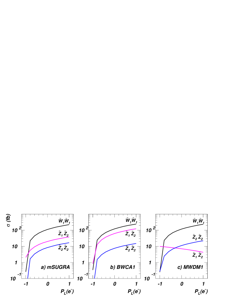
Figure 19: Cross sections for $e^{+}e^{-}\rightarrow\widetilde{W}_{1}^{+}\widetilde{W}_{1}^{-}$, $\widetilde{Z}_{1}\widetilde{Z}_{2}$ and $\widetilde{Z}_{2}\widetilde{Z}_{2}$ processes versus electron beam polarization $P_{L}(e^{-})$ for an electron-positron linear collider operating at $\sqrt{s}=500$ GeV for a) mSUGRA, b) BWCA1 and c) MWDM1 from Ref. [24]. The positron beam is taken to be unpolarized.

The dependence of the cross sections for $\widetilde{W}_{1}^{+}\widetilde{W}_{1}^{-}$, $\widetilde{Z}_{1}\widetilde{Z}_{2}$ and $\widetilde{Z}_{2}\widetilde{Z}_{2}$ production on the longitudinal polarization of the electron beam provides an additional tool at the ILC. This dependence is illustrated in Fig. 19 for the mSUGRA model in Table 2 in frame a), for case BWCA1 in frame b) and for case MWDM1, which is point 1 of Ref. [24]. In all three cases, the chargino and the second lightest neutralino have dominant wino components so that the magnitudes and the polarization depence of $\sigma(\widetilde{W}_{1}\widetilde{W}_{1})$ and $\sigma(\widetilde{Z}_{2}\widetilde{Z}_{2})$ are qualitatively similar to one another and to the corresponding dependence in the mSUGRA model[94]. A minor difference is that, for $P_{L}=-1$, $\sigma(\widetilde{Z}_{2}\widetilde{Z}_{2})$ does not fall to quite as small values for the MWDM1 case because its hypercharge gaugino component always remains significant, as we have already discussed. The polarization-dependence and/or the magnitude of the $e^{+}e^{-}\rightarrow\widetilde{Z}_{1}\widetilde{Z}_{2}$ process are, however, quite different in the three cases. In the limit that $\widetilde{Z}_{1}$ is a bino and $\widetilde{Z}_{2}$ is the wino (a good approximation in the mSUGRA case and an even better approximation in the BWCA case), $t$-channel selectron exchange dominates the amplitude. Recall, however, that for $P_{L}(e^{-})=1$ ($P_{L}(e^{-})=-1$) only $\tilde{e}_{L}$ ($\tilde{e}_{R}$) exchange is possible. Since the chargino is always wino-like, its couplings to $\tilde{e}_{R}$ are strongly suppressed, accounting for the behaviour of the cross sections in the first two frames. For the MWDM1 case in frame c), we would naively expect that $\widetilde{Z}_{1}$ would be photino-like and $\widetilde{Z}_{2}$ would be zino-like. It turns out, however, that (for the specific MWDM1 parameters) the difference $M_{1}({\rm weak})-M_{2}({\rm weak})$ is sufficiently large, and results in a flip of the relative sign between the gaugino components of both $\widetilde{Z}_{1}$ and $\widetilde{Z}_{2}$, while roughly preserving the magnitude. This strongly suppresses the $e\tilde{e}_{L}\widetilde{Z}_{1}$ coupling, and hence, the $\tilde{e}_{L}$ exchange amplitude, resulting in the relatively flat and even decreasing polarization-dependence of the cross section.

A very striking feature of the figure is the very large cross section for $\widetilde{Z}_{1}\widetilde{Z}_{2}$ production for a left polarized electron beam for the BWCA1 case in frame b), as compared with the mSUGRA case. In both cases, since $\widetilde{Z}_{1}$ and $\widetilde{Z}_{2}$ couple to (a not-so-heavy) $\tilde{e}_{L}$ mainly via their large hypercharge and $SU(2)$ gaugino components, respectively, $\tilde{e}_{L}$ exchange completely dominates $\widetilde{Z}_{1}\widetilde{Z}_{2}$ production at $P_{L}=1$. Moreover, the magnitudes of the couplings, as well as selectron masses, are very comparable in the two scenarios. The reason for the difference in the cross sections lies in the relative sign between the $\widetilde{Z}_{1}$ and $\widetilde{Z}_{2}$ eigenvalues (not physical masses) of the neutralino mass matrix. Since $M_{1}/M_{2}<0$, we expect this sign to flip in the BWCA case as compared with the mSUGRA or the MWDM cases, where $M_{1}/M_{2}$ is positive. This is relevant because when we square the $t$-channel amplitude and sum over the neutralino spins, there is one term that is proportional to the product $m_{\widetilde{Z}_{1}}m_{\widetilde{Z}_{2}}$ (see e.g. Eq. (8f) of Ref. [95], where the last term that includes the factor $(-1)^{\theta_{i}+\theta_{j}}$ is the one we are referring to). This term always flips sign between any scenario with positive $M_{1}/M_{2}$ vs. negative $M_{1}/M_{2}$. As a result, what was a significant cancellation in the mSUGRA case in frame a) of Fig. 19 turns into a sum in frame b), accounting for the factor $\sim 2.5$ increase in $\sigma(\widetilde{Z}_{1}\widetilde{Z}_{2})$ at $P_{L}=1$.

We examine this potential enhancement of the $e^{+}e^{-}\rightarrow\widetilde{Z}_{1}\widetilde{Z}_{2}$ production cross section at a $\sqrt{s}=0.5$ TeV linear collider in Fig. 20. In frame a), we show contours of $\sigma(e^{+}e^{-}\rightarrow\widetilde{Z}_{1}\widetilde{Z}_{2})$ in fb in the $m_{0}\ vs.\ m_{1/2}$ plane for $A_{0}=0$, $\tan\beta=10$ and $\mu>0$, in the case of the mSUGRA model. The light (yellow) shaded region is where either chargino pair production or selectron pair production is kinematically accessible at a $\sqrt{s}=0.5$ TeV ILC. We see that the $\widetilde{Z}_{1}\widetilde{Z}_{2}$ cross section only exceeds the 100 fb level at the very lowest values of $m_{0}$ and $m_{1/2}$, in the lower left corner. The cross section at the $\sim 10$ fb level gives some additional reach of an ILC for SUSY beyond the range where chargino pair production or slepton pair production are possible[94, 92]. In frame b), we show the same situation for the BWCA scenario where $M_{1}$ has been set to negative values everywhere in the $m_{0}\ vs.\ m_{1/2}$ plane such that the WMAP value $\Omega_{\widetilde{Z}_{1}}h^{2}=0.11$ is fulfilled. In this case, the $\widetilde{Z}_{1}\widetilde{Z}_{2}$ production cross section is in general increased everywhere, and exceeds 100 fb in a much larger region. Of course, the region of reaction kinematic accessibility has decreased somewhat due to the increase in $m_{\widetilde{Z}_{1}}$ for a given $m_{0}$ and $m_{1/2}$ value, so that contours of accessibility reach only up to $m_{1/2}\sim 350$ GeV (as opposed to $420$ GeV in the mSUGRA case). Also, the cross section falls off at large values of $m_{0}$ since the amplitude is suppressed with increasing selectron mass. In frame c), we show the same cross section in the $m_{0}\ vs.\ m_{1/2}$ plane, except here $M_{2}$ is taken negative, and is decreased at each point in absolute value until the WMAP value is obtained. In this case, the kinematically accessible region increases since for a given $m_{0}$ and $m_{1/2}$ value $m_{\widetilde{Z}_{2}}$ is lowered compared to the mSUGRA case, while $m_{\widetilde{Z}_{1}}$ stays fixed. Again, a rather large region appears with $\sigma>10-100$ fb, so that $\widetilde{Z}_{1}\widetilde{Z}_{2}$ production should be robust over much of parameter space in the BWCA scenario as long as $\widetilde{Z}_{1}\widetilde{Z}_{2}$ production is kinematically accessible and $m_{0}$ is not too large. An unexpectedly large value of $\sigma(\widetilde{Z}_{1}\widetilde{Z}_{2})/\sigma(\widetilde{W}_{1}\widetilde{W}_{1})$ may, therefore, be an indication that $M_{1}/M_{2}<0$ and that the selectrons are not too heavy.

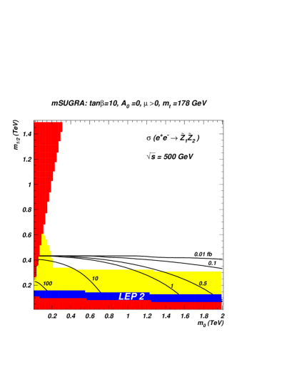
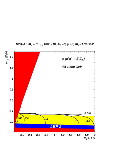
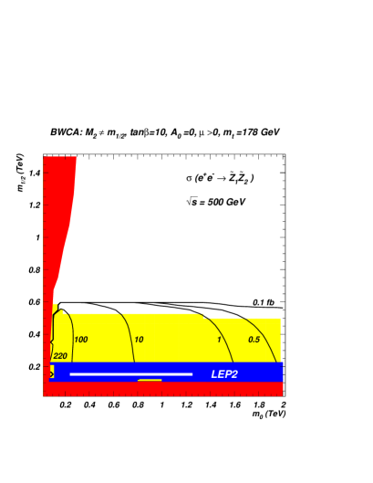
Figure 20: Contours of $\sigma(e^{+}e^{-}\rightarrow\widetilde{Z}_{1}\widetilde{Z}_{2})$ in fb for a $\sqrt{s}=0.5$ TeV ILC with unpolarized beams in the $m_{0}\ vs.\ m_{1/2}$ plane for $\tan\beta=10$, $A_{0}=0$, $\mu>0$ and a) mSUGRA model, b) $-M_{1}>m_{1/2}$ BWCA and c) $-M_{2}<m_{1/2}$ BWCA. The yellow shaded regions show where $\widetilde{W}_{1}^{+}\widetilde{W}_{1}^{-}$ and/or $\tilde{\ell}^{+}\tilde{\ell}^{-}$ should also be kinematically accessible to a $\sqrt{s}=0.5$ TeV ILC.

The rather large $e^{+}e^{-}\rightarrow\widetilde{Z}_{1}\widetilde{Z}_{2}$ cross section at the ILC potentially leads to another distinguishing feature of SUSY events at the ILC in the BWCA model: at least for $m_{0}\stackrel{{\scriptstyle<}}{{\sim}}1$ TeV, we should expect a large rate for events with one or more isolated photons due to the enhanced branching fraction for $\widetilde{Z}_{2}\rightarrow\widetilde{Z}_{1}\gamma$ decays. Thus, from $\widetilde{Z}_{1}\widetilde{Z}_{2}$ production, we may expect $\gamma+\not\!\!{E}$ events, while from $\widetilde{Z}_{2}\widetilde{Z}_{2}$ production, we may expect $\gamma\gamma+\not\!\!{E}$, $\gamma+jets+\not\!\!{E}$ events, $\gamma+\ell\bar{\ell}+\not\!\!{E}$ events and $\gamma+\not\!\!{E}$. Since the $\gamma$ arises from a two body decay, the endpoints of the $E(\gamma)$ distribution will be functions of $\sqrt{s},\ m_{\widetilde{Z}_{2}}$ and $m_{\widetilde{Z}_{1}}$. A measurement of the endpoints of this distribution will thus allow an independent measurement of the two lighter neutralino masses. The $E(\gamma)$ distribution is shown in Fig. 21 for BWCA2 at a $\sqrt{s}=0.5$ TeV ILC.

Figure 21: Distribution in $E(\gamma)$ from $e^{+}e^{-}\rightarrow\widetilde{Z}_{2}\widetilde{Z}_{1}$ with $\widetilde{Z}_{2}\rightarrow\gamma\widetilde{Z}_{1}$ for point BWCA2 in $e^{+}e^{-}$ collisions at $\sqrt{s}=0.5$ TeV.

6 Conclusions

In this paper, we have considered the phenomenological implications of neutralino dark matter in the bino-wino co-annihilation (BWCA) scenario, and compared these to the case of mixed wino dark matter which has a qualitatively similar spectrum. The BWCA scenario arises in models with non-universal gaugino masses where, at the weak scale, $|M_{1}|\sim|M_{2}|$, but where the two gauginos masses have opposite signs. The same sign case gives rise to mixed wino dark matter, while in the BWCA case, there is little mixing so that the $\widetilde{Z}_{1}$ remains nearly a pure bino, while $\widetilde{Z}_{2}$ remains nearly a pure wino. The scenario can be brought into accord with the WMAP $\Omega_{\widetilde{Z}_{1}}h^{2}\sim 0.11$ constraint by arranging for $m_{\widetilde{W}_{1}}\sim m_{\widetilde{Z}_{2}}\sim m_{\widetilde{Z}_{1}}$, so that bino-wino co-annihilation is the dominant neutralino annihilation mechanism in the early universe.

Since co-annihilation processes are the dominant mechanism for the annihilation of relic neutralinos from the Big Bang, it is expected that indirect dark matter detection rates (which depend on the $\widetilde{Z}_{1}\widetilde{Z}_{1}$ pair-annihilation cross section) will typically be quite low in the BWCA scenario. Direct detection of neutralinos may be possible for BWCA DM at stage 3 detectors in some portions of parameter space. In contrast, for the MWDM case, neutralino annihilation cross sections are enhanced relative to mSUGRA so that it is more likely that an indirect signal for DM will be seen. If we already have some infomation about the sparticle spectrum from the LHC, it may be that results from direct and indirect DM detection experiments may serve to discriminate between these scenarios.

The small mass gap expected between $m_{\widetilde{Z}_{2}}$ and $m_{\widetilde{Z}_{1}}$ is a hallmark of both the BWCA and the MWDM scenarios, and leads to a variety of interesting consequences for collider experiments. In teh BWCA case, if $m_{0}\stackrel{{\scriptstyle<}}{{\sim}}1$ TeV, then the radiative decay $\widetilde{Z}_{2}\rightarrow\widetilde{Z}_{1}\gamma$ is greatly enhanced, leading to the production of isolated photons at the Tevatron, LHC and ILC. While extraction of the isolated photon signal above SM background looks difficult at the Tevatron, they should yield observable signals at the CERN LHC. The LHC should also be able to extract the $m_{\widetilde{Z}_{2}}-m_{\widetilde{Z}_{1}}$ mass difference from gluino and squark cascade decay events which contain isolated opposite sign/same flavor dilepton pairs. By comparing the neutralino mass difference to measurements of the gluino mass, we should readily be able to infer that the weak scale gaugino masses are incompatible with expectation from models with a universal gaugino mass at the high scale. At the ILC, again small $m_{\widetilde{W}_{1}}-m_{\widetilde{Z}_{1}}$ and $m_{\widetilde{Z}_{2}}-m_{\widetilde{Z}_{1}}$ mass gaps should be measurable, as in the MWDM and MHDM scenarios. It should also be possible to extract the weak scale values of the gaugino mass parameters. However, in the case of BWCA, $\widetilde{Z}_{1}\widetilde{Z}_{2}$ production should occur at enhanced rates relative to mSUGRA and MWDM, with a production cross section which increases with $P_{L}(e^{-})$. In constrast to MHDM, the $\widetilde{Z}_{3}$ and $\widetilde{Z}_{4}$ states will typically occur at much higher mass scales associated with large values for the $|\mu|$ parameter.

Appendix: Effective Theories in Quantum Mechanics

Consider a situation where the total Hamiltonian can be split into two pieces,

$$H=H_{0}+V,$$

so that the spectrum of $H_{0}$ is hierarchical, i.e., it consists of “low energy” states $|l_{i}\rangle$, possibly interacting with one another via interactions included in $H_{0}$, and “high energy” states, $|h_{a}\rangle$ (again possibly interacting with themselves via interactions included in $H_{0}$). Without loss of generality, all interactions between the states $\left\{|l_{i}\rangle\right\}$ and the states $\left\{|h_{a}\rangle\right\}$ are encapsulated in $V$. In other words, $\langle h_{a}|H_{0}|l_{i}\rangle=0$, and $\langle l_{i}|V|l_{j}\rangle=\langle h_{a}|V|h_{b}\rangle=0$.

We seek a description of low energy states in terms of an effective Hamiltonian $H_{\rm eff}$, that acts only on the low energy states $\left\{|l_{i}\rangle\right\}$, assuming that we are at energies that are too low to excite the high energy states. Note that even if $H_{0}$ is completely diagonal in the low energy sector, we would expect that scattering of low energy states (with energy $E\ll M_{a}$) would occur via their interactions with the high energy sector, with an amplitude suppressed by $E/M_{a}$. Here, we show how this comes about and obtain an expression for $H_{\rm eff}$.

We define $H_{\rm eff}$ by matching the low energy Green’s functions of the full theory with those of the effective theory,

$$\langle l_{i}|\frac{1}{H_{0}+V-z}|l_{j}\rangle\equiv\langle l_{i}|\frac{1}{H_{\rm eff}-z}|l_{j}\rangle,\ \ \ {\rm if}\ |z|\ll M_{a}.$$ (17)

Here, $z$ is the complex argument of the Green’s function. Expanding the left hand side of (17), we obtain

$$\langle l_{i}|\frac{1}{H_{\rm eff}-z}|l_{j}\rangle = \langle l_{i}|\frac{1}{H_{0}-z}|l_{j}\rangle+\langle l_{i}|\frac{1}{H_{0}-z}(-V)\frac{1}{H_{0}-z}|l_{j}\rangle$$ (18)

$$+ \langle l_{i}|\frac{1}{H_{0}-z}(-V)\frac{1}{H_{0}-z}(-V)\frac{1}{H_{0}-z}|l_{j}\rangle+\cdots.$$

Clearly, if $V=0$ (no interactions between low and high energy states), $H_{\rm eff}$ is just $H_{0}$ restricted to the low energy subspace, i.e. $H_{\rm eff}=H_{0}{\cal P}_{\rm low}$, where ${\cal P}_{\rm low}$ is the projector on to the low energy subspace. It is also clear that terms with an odd number of $(-V)$ factors on the right hand side of (18) are all zero because $V$ only connects states in the low energy sector with those in the high energy sector, whereas $H_{0}$ only connects low energy (high energy) states with one another. The third term on the right hand side of (18) can be written as

$$\left(\frac{1}{H_{0}-z}\right)_{ii^{\prime}}(-V)_{i^{\prime}a}\left(\frac{1}{H_{0}-z}\right)_{ab}(-V)_{bj^{\prime}}\left(\frac{1}{H_{0}-z}\right)_{j^{\prime}j},$$

with the repeated indices $i^{\prime},a,b$ and $j^{\prime}$ all summed up. We now defined an induced effective potential $V^{\rm induced}$ by,

$$-\left(V^{\rm induced}\right)_{i^{\prime}j^{\prime}}=(-V)_{i^{\prime}a}\left(\frac{1}{H_{0}-z}\right)_{ab}(-V)_{bj^{\prime}},$$ (19)

in terms of which this term can be written as,

$$\left(\frac{1}{H_{0}-z}\right)_{ii^{\prime}}\left(-V^{\rm induced}\right)_{i^{\prime}j^{\prime}}\left(\frac{1}{H_{0}-z}\right)_{j^{\prime}j}.$$

In exactly the same manner, the term with four factors of $(-V)$ will end up as one with two factors of $\left(-V^{\rm induced}\right)$, etc. so that we have a geometric series that can be summed to give

$$\langle l_{i}|\frac{1}{H_{\rm eff}-z}|l_{j}\rangle=\langle l_{i}|\frac{1}{H_{0}+V^{\rm induced}-z}|l_{j}\rangle,$$ (20)

showing that the interactions between the low and high sectors effectively induce an additional “potential” in the low sector.

Up to now, our considerations (though formal) have been “exact” in the sense that we have not made any low energy approximation. This shows up in the fact that the “potential” $V^{\rm induced}$ defined in (19) depends on the “energy” $z$. If $|z|$ is small compared with the high energy scale associated with the spectrum of $H_{0}$, we can ignore it in the evaluation of the matrix elements of $(H_{0}-z)^{-1}$ between high energy states, and approximate $V^{\rm induced}$ by,

$$\left(V^{\rm induced}\right)_{ij} = -\sum_{a,b}\left[V_{ia}\left(\frac{1}{H_{0}}\right)_{ab}V_{bj}+V_{ia}{\cal O}(\frac{|z|}{M_{a}^{2}})V_{bj}+\cdots\right]$$ (21)

$$\simeq -\sum_{a,b}V_{ia}\left(\frac{1}{H_{0}}\right)_{ab}V_{bj},$$

where, in the last step, we have made the “low energy approximation” and obtained what is a conventional potential (independent of $z$). Assuming that the matrix elements $V_{ia}$ have magnitudes corresponding to the low energy scale, we see that the $\left(\frac{1}{H_{0}}\right)_{ab}$ term supresses the low energy matrix elements of $V^{\rm induced}$ by $|z|/M_{a}$ as expected.

This expression is particularly useful in two cases.

1. If $H_{0}{\cal P}_{\rm low}$ is diagonal, then all interactions arise only from $V^{\rm induced}$ and this analysis is essential to obtain any scattering in the low energy sector.

2. If the low energy sector has an approximate symmetry that is violated only by its interactions with the high mass sector, or even just by interactions solely within the high mass sector, we can use $V^{\rm induced}$ to study these symmetry violations.

In the analysis up to now, we have retained just the leading correction in powers of $M_{a}$. It is straightforward to retain the ${\cal O}(1/M_{a}^{2})$ term in the expansion of the Green’s function $(H_{\rm eff}-z)^{-1}$. The energy eigenvalues $E$ in the low energy theory are given by those values of $z$ where the corresponding Green’s function develops a singularity,i.e., where

$$H_{\rm eff}|\psi\rangle=E|\psi\rangle.$$

Assuming, for simplicity, that $H_{0}$ is diagonal in the high mass sector and retaining terms to ${\cal O}(1/M_{a}^{2})$, we find that these eigenvalues are given by the generalized matrix eigenvalue equation,

$$\sum_{j}[(H_{0})_{ij}-\sum_{a}V_{ia}\frac{1}{M_{a}}V_{aj}]c_{j}=E\sum_{j}[\delta_{ij}+\sum_{a}V_{ia}\frac{1}{M_{a}^{2}}V_{aj}]c_{j}.$$ (22)

The positive operator on the right hand side serves as a metric in the low energy subspace.

This formalism can be directly used to obtain the eigenvalues (8) of the neutralino mas matrix in the large $|\mu|$ limit. In this case, the low energy sector comprises of the neutral wino and the bino, and the generalized eigenvalue equation takes the form,

$$\left(\begin{array}[]{cc}M_{2}+a&-a\tan\theta_{W}\\ -a\tan\theta_{W}&M_{1}+a\tan^{2}\theta_{W}\end{array}\right)\left(\begin{array}[]{c}c_{1}\\ c_{2}\end{array}\right)=E\left(\begin{array}[]{cc}1+\frac{M_{W}^{2}}{\mu^{2}}&-\frac{M_{W}^{2}}{\mu^{2}}\tan\theta_{W}\\ -\frac{M_{W}^{2}}{\mu^{2}}\tan\theta_{W}&1+\frac{M_{W}^{2}}{\mu^{2}}\tan^{2}\theta_{W}\end{array}\right)\left(\begin{array}[]{c}c_{1}\\ c_{2}\end{array}\right),$$ (23)

with $a\equiv\frac{M_{W}^{2}}{\mu}\sin 2\beta$ much smaller than $M_{1}$ and $M_{2}$ in the large $|\mu|$ limit.

References

- [1] For recent reviews, see e.g. C. Jungman, M. Kamionkowski and K. Griest,Phys. Rept. 267 (195) 1996; A. Lahanas, N. Mavromatos and D. Nanopoulos, Int. J. Mod. Phys. D 12 (2003) 1529; M. Drees, hep-ph/0410113; K. Olive, “Tasi Lectures on Astroparticle Physics”, astro-ph/0503065.
- [2] P. Gondolo, J. Edsjo, P. Ullio, L. Bergstrom, M. Schelke and E. A. Baltz, JCAP 0407, 008 (2004); G. Belanger, F. Boudjema, A. Pukhov and A. Semenov, Comput. Phys. Commun. 149 (2002) 103.
- [3] IsaRED, by H. Baer, C. Balazs and A. Belyaev, J. High Energy Phys. 0203 (2002) 042.
- [4] D. N. Spergel et al., astro-ph/0302209; C. L. Bennett et al., astro-ph/0302207.
- [5] J. Ellis, K. Olive, Y. Santoso and V. Spanos, Phys. Lett. B 565 (2003) 176; H. Baer and C. Balazs, JCAP05 (2003) 006; U. Chattapadhyay, A. Corsetti and P. Nath, Phys. Rev. D 68 (2003) 035005; A. Lahanas and D. V. Nanopoulos, Phys. Lett. B 568 (2003) 55; for a review, see A. Lahanas, N. Mavromatos and D. Nanopoulos, Int. J. Mod. Phys. D 12 (2003) 1529.
- [6] A. Chamseddine, R. Arnowitt and P. Nath, Phys. Rev. Lett. 49 (1982) 970; R. Barbieri, S. Ferrara and C. Savoy, Phys. Lett. B 119 (1982) 343; N. Ohta, Prog. Theor. Phys. 70 (1983) 542; L. J. Hall, J. Lykken and S. Weinberg, Phys. Rev. D 27 (1983) 2359; for reviews, see H. P. Nilles, Phys. Rep. 110 (1984) 1, and P. Nath, hep-ph/0307123.
- [7] H. Goldberg, Phys. Rev. Lett. 50 (1419) 1983; J. Ellis, J. Hagelin, D. Nanopoulos and M. Srednicki, Phys. Lett. B127, 233 (1983); J. Ellis, J. Hagelin, D. Nanopoulos, K. Olive and M. Srednicki, Nucl. Phys. B238, 453 (1984).
- [8] H. Baer and M. Brhlik, Phys. Rev. D 53 (1996) 597; V. Barger and C. Kao, Phys. Rev. D 57 (1998) 3131.
- [9] J. Ellis, T. Falk and K. Olive, Phys. Lett. B 444 (1998) 367; J. Ellis, T. Falk, K. Olive and M. Srednicki, Astropart. Phys. 13 (2000) 181; M.E. Gómez, G. Lazarides and C. Pallis, Phys. Rev. D 61 (2000) 123512 and Phys. Lett. B 487 (2000) 313; A. Lahanas, D. V. Nanopoulos and V. Spanos, Phys. Rev. D 62 (2000) 023515; R. Arnowitt, B. Dutta and Y. Santoso, Nucl. Phys. B 606 (2001) 59; see also Ref. [3]
- [10] K. L. Chan, U. Chattopadhyay and P. Nath, Phys. Rev. D 58 (1998) 096004. J. Feng, K. Matchev and T. Moroi, Phys. Rev. Lett. 84 (2000) 2322 and Phys. Rev. D 61 (2000) 075005; see also H. Baer, C. H. Chen, F. Paige and X. Tata, Phys. Rev. D 52 (1995) 2746 and Phys. Rev. D 53 (1996) 6241; H. Baer, C. H. Chen, M. Drees, F. Paige and X. Tata, Phys. Rev. D 59 (1999) 055014; for a model-independent approach, see H. Baer, T. Krupovnickas, S. Profumo and P. Ullio, J. High Energy Phys. 0510 (2005) 020.
- [11] M. Drees and M. Nojiri, Phys. Rev. D 47 (1993) 376; H. Baer and M. Brhlik, Phys. Rev. D 57 (1998) 567 and Ref. [8]; H. Baer, M. Brhlik, M. Diaz, J. Ferrandis, P. Mercadante, P. Quintana and X. Tata, Phys. Rev. D 63 (2001) 015007; J. Ellis, T. Falk, G. Ganis, K. Olive and M. Srednicki, Phys. Lett. B 510 (2001) 236; L. Roszkowski, R. Ruiz de Austri and T. Nihei, J. High Energy Phys. 0108 (024) 2001; A. Djouadi, M. Drees and J. L. Kneur, J. High Energy Phys. 0108 (2001) 055; A. Lahanas and V. Spanos, Eur. Phys. J. C 23 (2002) 185.
- [12] R. Arnowitt and P. Nath, Phys. Rev. Lett. 70 (1993) 3696; H. Baer and M. Brhlik, Ref. [8]; A. Djouadi, M. Drees and J. Kneur, Phys. Lett. B 624 (2005) 60.
- [13] C. Böhm, A. Djouadi and M. Drees, Phys. Rev. D 30 (2000) 035012; J. R. Ellis, K. A. Olive and Y. Santoso, Astropart. Phys. 18 (2003) 395; J. Edsjö, et al., JCAP 04 (2003) 001
- [14] H. Baer, A. Belyaev, T. Krupovnickas and A. Mustafayev, J. High Energy Phys. 0406 (2004) 044.
- [15] H. Baer, A. Mustafayev, S. Profumo, A. Belyaev and X. Tata, Phys. Rev. D 71 (2005) 095008 and J. High Energy Phys. 0507 (2005) 065.
- [16] D. Auto, H. Baer, A. Belyaev and T. Krupovnickas, J. High Energy Phys. 0410 (2004) 066.
- [17] S. Profumo, Phys. Rev. D 68 (2003) 015006
- [18] J. Ellis, K. Olive and Y. Santoso, Phys. Lett. B 539 (2002) 107; J. Ellis, T. Falk, K. Olive and Y. Santoso, Nucl. Phys. B 652 (2003) 259.
- [19] M. Drees, hep-ph/0410113.
- [20] A. Brignole, L. E. Ibanez and C. Munoz, Nucl. Phys. B 422 (1994) 125 [Erratum-ibid. B 436 (1995) 747]; . Brignole, L. E. Ibanez, C. Munoz and C. Scheich, Z. Physik C 74 (1997) 157.
- [21] C. H. Chen, M. Drees and J. Gunion, Phys. Rev. D 55 (1997) 330, Erratum-ibid. D 60 (1999) 039901.
- [22] R. Dermisek and A. Mafi, Phys. Rev. D 65 (2002) 055002; H. Baer, C. Balazs, A. Belyaev, R. Dermisek, A. Mafi and A. Mustafayev, J. High Energy Phys. 0205 (2002) 061; C. Balazs and R. Dermisek, J. High Energy Phys. 0306 (2003) 024.
- [23] H. Baer, M. Diaz, P. Quintana and X. Tata, J. High Energy Phys. 0004 (2000) 016.
- [24] H. Baer, A. Mustafayev, E. Park and S. Profumo, J. High Energy Phys. 0507 (2005) 046.
- [25] L. Randall and R. Sundrum, Nucl. Phys. B 557 (1999) 79; G. Giudice, M. Luty, H. Murayama and R. Rattazzi, J. High Energy Phys. 9812 (1998) 27.
- [26] J. Amundsen et al., hep-ph/9609374; G. Anderson, H. Baer, C. H. Chen and X. Tata, Phys. Rev. D 61 (2000) 095005.
- [27] N. Chamoun, C. S. Huang, C. Liu and X. Wu, Nucl. Phys. B 624 (2002) 81.
- [28] U. Chattapadhyay, A. Corsetti and P. Nath, Phys. Rev. D 66 (2002) 035003.
- [29] K. Griest and L. Roszkowski, Phys. Rev. D 46 (1992) 3309.
- [30] T. Moroi and L. Randall, Nucl. Phys. B 570 (2000) 455.
- [31] A. Corsetti and P. Nath, Phys. Rev. D 64 (2001) 125010.
- [32] A. Birkedal-Hansen and B. Nelson, Phys. Rev. D 64 (2001) 015008 and Phys. Rev. D 67 (2003) 095006.
- [33] V. Bertin, E. Nezri and J. Orloff, J. High Energy Phys. 0302 (2003) 046.
- [34] A. Bottino, F. Donato, N. Fornengo and S. Scopel, Phys. Rev. D 70 (2004) 015005.
- [35] G. Belanger, F. Boudjema, A. Cottrant, A. Pukhov and A. Semenov, Nucl. Phys. B 706 (2005) 411.
- [36] D. Cerdeno and C. Munoz, J. High Energy Phys. 0410 (2004) 015; Y. Mambrini and C. Munoz, JCAP 0410 (2004) 003 and hep-ph/0507263; see also S. Baek, D. Cerdeno, Y. G. Kim, P. Ko and C. Munoz, hep-ph/0505019.
- [37] A. Masiero, S. Profumo and P. Ullio, Nucl. Phys. B 712 (2005) 86.
- [38] H. Baer and X. Tata, Weak Scale Supersymmetry: From Superfields to Scattering Events, (Cambridge University Press, 2006).
- [39] ISAJET v7.72, by H. Baer, F. Paige, S. Protopopescu and X. Tata, hep-ph/0312045.
- [40] E. Boos et al. (CompHEP Collaboration), Nucl. Instrum. Meth. A534 (2004) 250.
- [41] P. Gondolo and G. Gelmini, Nucl. Phys. B 360 (1991) 145; J. Edsjo and P. Gondolo, Phys. Rev. D 56 (1997) 1879.
- [42] H. Baer, V. Barger, D. Karatas and X. Tata, Phys. Rev. D 36 (1987) 96.
- [43] K. Griest and D. Seckel, Phys. Rev. D 43 (1991) 3191.
- [44] J. L. Feng, T. Moroi, L. Randall, M. Strassler and S. f. Su, Phys. Rev. Lett. 83 (1999) 1731.
- [45] J. Edsjo, M. Schelke, P. Ullio and P. Gondolo, JCAP 0304 (2003) 001 [arXiv:hep-ph/0301106].
- [46] S. Profumo, arXiv:astro-ph/0508628, Phys. Rev. D, in press.
- [47] S. Profumo and C. E. Yaguna, Phys. Rev. D 69 (2004) 115009 [arXiv:hep-ph/0402208].
- [48] For a review, see e.g. G. Eigen, R. Gaitskell, G. Kribs and K. Matchev, hep-ph/0112312; see also D. Hooper and L. T. Wang, Phys. Rev. D 69 (2004) 035001; W. de Boer, M. Herold, C. Sander and V. Zhukov, hep-ph/0309029.
- [49] P. Gondolo, J. Edsjo, P. Ullio, L. Bergstrom, M. Schelke and E. A. Baltz, astro-ph/0211238.
- [50] J.F. Navarro et al., Mon. Not. Roy. Astron. Soc. 349 (2004) 1039, astro-ph/0311231; the adiabatic contraction of the halo follows Blumental et al., Astrophys. J. 301 (1986) 27. For the halo parameter choices see also ref. [53].
- [51] H. Baer and J. O’Farrill, JCAP03, 012 (2004).
- [52] H. Baer, A. Belyaev, T. Krupovnickas and J. O’Farrill, JCAP 0404 (2004) 005.
- [53] S. Profumo and P. Ullio, JCAP 0407 (2004) 006.
- [54] For a recent analysis, see H. Baer, C. Balazs, A. Belyaev and J. O’Farrill, JCAP0309, 2003 (007); a subset of earlier work includes M. Goodman and E. Witten, Phys. Rev. D 31 (1985) 3059; K. Griest, Phys. Rev. Lett. 61 (1988) 666 and Phys. Rev. D 38 (1988) 2357 [Erratum-ibid. D 39, 3802 (1989)]; M. Drees and M. Nojiri, Phys. Rev. D 47 (1993) 4226 and Phys. Rev. D 48 (1993) 3483; V. A. Bednyakov, H. V. Klapdor-Kleingrothaus and S. Kovalenko, Phys. Rev. D 50 (1994) 7128; P. Nath and R. Arnowitt, Phys. Rev. Lett. 74 (1995) 4592; L. Bergstrom and P. Gondolo, Astropart. Phys. 5 (1996) 263; H. Baer and M. Brhlik, Phys. Rev. D 57 (1998) 567; J. Ellis, A. Ferstl and K. Olive, Phys. Lett. B 481 (2000) 304 and Phys. Rev. D 63 (2001) 065016; E. Accomando, R. Arnowitt, B. Dutta and Y. Santoso, Nucl. Phys. B 585 (2000) 124; A. Bottino, F. Donato, N. Fornengo and S. Scopel, Phys. Rev. D 63 (2001) 125003; M. E. Gomez and J. D. Vergados, Phys. Lett. B 512 (2001) 252; A. B. Lahanas, D. V. Nanopoulos and V. C. Spanos, Phys. Lett. B 518 (2001) 94; A. Corsetti and P. Nath, Phys. Rev. D 64 (2001) 115009; E. A. Baltz and P. Gondolo, Phys. Rev. Lett. 86 (2001) 5004; M. Drees, Y. G. Kim, T. Kobayashi and M. M. Nojiri, Phys. Rev. D 63 (2001) 115009; see also J. Feng, K. Matchev and F. Wilczek, Phys. Lett. B 482 (2000) 388 and Phys. Rev. D 63 (2001) 045024; R. Ellis, A. Ferstl, K. A. Olive and Y. Santoso, Phys. Rev. D 67 (2003) 123502; J. R. Ellis, K. A. Olive, Y. Santoso and V. C. Spanos, Phys. Rev. D 69 (2004) 015005; see C. Munoz, hep-ph/0309346 for a recent review.
- [55] See H. Baer, C. Balazs, A. Belyaev and J. O’Farrill, Ref. [54]
- [56] D. S. Akerib et al. (CDMS Collaboration), astro-ph/0405033 (2004).
- [57] A. Benoit et al. (Edelweiss Collaboration), Phys. Lett. B 545 (2002) 43.
- [58] M. Bravin et al. (CRESST Collaboration), Astrophys. J. 12 (1999) 107.
- [59] N. Spooner et al. (Zeplin-1Collaboration), in Proc. of the APS/DPF/DPB Summer Study on the Future of Particle Physics (Snowmass 2001) ed. N. Graf, eConf C010630, E601 (2001).
- [60] Y. Suzuki et al. (Xenon Colaboration), hep-ph/0008296.
- [61] I. Abt et al., hep-ex/0404039.
- [62] D. B. Cline et al. (ZEPLIN-4 Collaboration), Nucl. Phys. 124 (Proc. Suppl.) (2003) 229.
- [63] See talk by C. Rubbia at 6th UCLA Symposium on Sources and Detection of Dark Matter and Dark Energy in the Universe, Marina del Ray, CA, February (2004).
- [64] J. Silk, K. Olive and M. Srednicki, Phys. Rev. Lett. 55 (1985) 257; K. Freese, Phys. Lett. B 167 (1986) 295; L. Krauss, M. Srednicki and F. Wilczek, Phys. Rev. D 33 (1986) 2079; V. Berezinsky, A. Bottino, J. R. Ellis, N. Fornengo, G. Mignola and S. Scopel, Astropart. Phys. 5 (1996) 333; L. Bergstrom, J. Edsjo and P. Gondolo, Phys. Rev. D 55 (1997) 1765 and Phys. Rev. D 58 (1998) 103519; A. Bottino, F. Donato, N. Fornengo and S. Scopel, Astropart. Phys. 10 (1999) 203; A. Corsetti and P. Nath, Int. J. Mod. Phys. A 15 (2000) 905; V. Barger, F. Halzen, D. Hooper and C. Kao, Phys. Rev. D 65 (2002) 075022; V. Bertin, E. Nezri and J. Orloff, Eur. Phys. J. C 26 (2002) 111 and J. High Energy Phys. 0302 (2003) 046.
- [65] E. Carmona et al., (Antares Collaboration), Nucl. Phys. 95 (Proc. Suppl.) (2001) 161.
- [66] J. Ahrens et al., (IceCube Collaboration), Nucl. Phys. 118 (Proc. Suppl.) (2003) 388; F. Halzen, astro-ph/0311004; F. Halzen and D. Hooper, JCAP0401 (2004) 002.
- [67] F. Stecker, Phys. Lett. B 201 (1988) 529; F. W. Stecker and A. J. Tylka, Astrophys. J. 343 (1989) 169; S. Rudaz and F. Stecker, Astrophys. J. 368 (1991) 406; M. Urban et al., Phys. Lett. B 293 (1992) 149; V. Berezinsky, A. Gurevich and K. Zybin, Phys. Lett. B 294 (1992) 221; V. Berezinsky, A. Bottino and G. Mignola, Phys. Lett. B 325 (1994) 136; L. Bergstrom, P. Ullio and J. H. Buckley, Astropart. Phys. 9 (1998) 137; L. Bergstrom, J. Edsjö and P. Ullio, Phys. Rev. D 58 (1998) 083507; J. Buckley et al., astro-ph/0201160; P. Ullio, L. Bergstrom, J. Edsjö and C. Lacey, Phys. Rev. D 66 (2002) 123502.
- [68] H. A. Mayer-Hasselwander et al. (EGRET Collaboration), MPE-440 (1998).
- [69] A. Morselli et al., (GLAST Collaboration), Nucl. Phys. 113 (Proc. Suppl.) (2002) 213.
- [70] S. Rudaz and F. Stecker, Astrophys. J. 325 (1988) 16; A. Tylka, Phys. Rev. Lett. 63 (1989) 840; M. Turner and F. Wilczek, Phys. Rev. D 42 (1990) 1001; M. Kamionkowski and M. Turner, Phys. Rev. D 43 (1991) 1774; A. Moskalenko and A. Strong, Phys. Rev. D 60 (1999) 063003; E. Baltz and J. Edsjö, Phys. Rev. D 59 (1999) 023511; G. Kane, L. T. Wang and J. Wells, Phys. Rev. D 65 (2002) 057701; E. Baltz, J. Edsjo, K. Freese and P. Gondolo, Phys. Rev. D 65 (2002) 063511; G. Kane, L. T. Wang and T. Wang, Phys. Lett. B 536 (2002) 263; D. Hooper, J. Taylor and J. Silk, hep-ph/0312076.
- [71] M. A. DuVernois et al. (HEAT Collaboration), Astrophys. J. 559 (2001) 296.
- [72] M. Pearce (Pamela Collaboration), Nucl. Phys. 113 (Proc. Suppl.) (2002) 314.
- [73] J. Casaus et al. (AMS Collaboration), Nucl. Phys. 114 (Proc. Suppl.) (2003) 259.
- [74] F. Stecker, S. Rudaz and T. Walsh, Phys. Rev. Lett. 55 (1985) 2622; F. Stecker and A. J. Tylka, Astrophys. J. 336 (1989) L51; P. Chardonnet, Mignola, P. Salati and R. Taillet, Phys. Lett. B 384 (1996) 161; A. Bottino, F. Donato, N. Fornengo and P. Salati, Phys. Rev. D 58 (1998) 123503; L. Bergstrom, J. Edsjo and P. Ullio, Astrophys. J. 526 (1999) 215.
- [75] S. Orito et al. (BESS Collaboration), Phys. Rev. Lett. 84 (2000) 1078.
- [76] H. Fuke et al. (BESS Collaboration), astro-ph/0504361.
- [77] K. Mori, C. J. Hailey, E. A. Baltz, W. W. Craig, M. Kamionkowski, W. T. Serber and P. Ullio, Astrophys. J. 566 (2002) 604.
- [78] S. Profumo and C.E. Yaguna, Phys. Rev. D 70 (2004) 095004
- [79] H. Baer and S. Profumo, astro-ph/0510722.
- [80] H. Komatsu and H. Kubo, Phys. Lett. B 157 (1985) 90 and Nucl. Phys. B 263 (1986) 265; H. E. Haber, G. Kane and M. Quiros, Phys. Lett. B 160 (1985) 297 and Nucl. Phys. B 273 (1986) 333; G. Gamberini, Z. Physik C 30 (1986) 605; R. Barbieri, G. Gamberini, G. F. Giudice and G. Ridolfi, Nucl. Phys. B 296 (1988) 75.
- [81] H. E. Haber and D. Wyler, Nucl. Phys. B 323 (1989) 267.
- [82] S. Ambrosanio and B. Mele, Phys. Rev. D 53 (1996) 2541 and Phys. Rev. D 55 (1997) 1399 [Erratum-ibid. D56, 3157 (1997)].
- [83] H. Baer and T. Krupovnickas, J. High Energy Phys. 0209 (2002) 038.
- [84] H. Baer, J. Ellis, G. Gelmini, D. V. Nanopoulos and X. Tata, Phys. Lett. B 161 (1985) 175; G. Gamberini, Z. Physik C 30 (1986) 605; H. Baer, V. Barger, D. Karatas and X. Tata, Phys. Rev. D 36 (1987) 96; H. Baer, X. Tata and J. Woodside, Phys. Rev. D 45 (1992) 142.
- [85] H. Baer, K. Hagiwara and X. Tata, Phys. Rev. D 35 (1987) 1598; H. Baer, D. Dzialo-Karatas and X. Tata, Phys. Rev. D 42 (1990) 2259; H. Baer, C. Kao and X. Tata, Phys. Rev. D 48 (1993) 5175; H. Baer, C. H. Chen, F. Paige and X. Tata, Phys. Rev. D 50 (1994) 4508.
- [86] I. Hinchliffe et al., Phys. Rev. D 55 (1997) 5520 and Phys. Rev. D 60 (1999) 095002; H. Bachacou, I. Hinchliffe and F. Paige, Phys. Rev. D 62 (2000) 015009; Atlas Collaboration, LHCC 99-14/15.
- [87] D. Dicus, S. Nandi and X. Tata, Phys. Lett. B 129 (1983) 451; A. Chamseddine, P. Nath and R. Arnowitt, Phys. Lett. B 129 (1983) 445; H. Baer and X. Tata,Phys. Lett. B 155 (1985) 278; H. Baer, K. Hagiwara and X. Tata, Phys. Rev. Lett. 57 (1986) 294 and Phys. Rev. D 35 (1987) 1598; R. Arnowitt and P. Nath, Mod. Phys. Lett. A 2 (1987) 331; R. Barbieri, F. Caravaglios, M. Frigeni and M. Mangano, Nucl. Phys. B 367 (1991) 28; H. Baer and X. Tata, Phys. Rev. D 47 (1993) 2739; J. Lopez, D. Nanopoulos, X. Wang and A. Zichichi, Phys. Rev. D 48 (1993) 2062 and Phys. Rev. D 52 (1995) 142; H. Baer, C. Kao and X. Tata, Phys. Rev. D 48 (1993) 5175; S. Mrenna, G. Kane, G. Kribs and J. Wells, Phys. Rev. D 53 (1996) 1168; H. Baer, C. H. Chen, F. Paige and X. Tata, Phys. Rev. D 54 (1996) 5866; V. Barger, C. Kao and T. Li,Phys. Lett. B 433 (1998) 328; K. Matchev and D. Pierce, Phys. Rev. D 60 (1999) 075004; H. Baer, C. H. Chen, M. Drees, F. Paige and X. Tata, Phys. Rev. Lett. 79 (1997) 986 and Phys. Rev. D 58 (1998) 075008; J. Lykken and K. Matchev, Phys. Rev. D 61 (2000) 015001.
- [88] H. Baer, M. Drees, F. Paige, P. Quintana and X. Tata, Phys. Rev. D 61 (2000) 095007; V. Barger and C. Kao, Phys. Rev. D 60 (1999) 115015; K. Matchev and D. Pierce, Phys. Lett. B 467 (1999) 225; H. Baer, T. Krupovnickas and X. Tata, J. High Energy Phys. 0307 (2003) 020.
- [89] H. Baer, J. Ellis, G. Gelmini, D. Nanopoulos and X. Tata, Phys. Lett. B 161 (1985) 175; G. Gamberini, Z. Physik C 30 (1986) 605; H. Baer, V. Barger, D. Karatas and X. Tata, Ref. [42]; H. Baer, X. Tata and J. Woodside, Phys. Rev. D 45 (1992) 142.
- [90] H. Baer, C. Balazs, A. Belyaev, T. Krupovnickas and X. Tata, J. High Energy Phys. 0306 (2003) 054. For earlier work, see H. Baer, C. H. Chen, F. Paige and X. Tata, Phys. Rev. D 52 (1995) 2746 and Phys. Rev. D 53 (1996) 6241; H. Baer, C. H. Chen, M. Drees, F. Paige and X. Tata, Phys. Rev. D 59 (1999) 055014; S. Abdullin and F. Charles, Nucl. Phys. B 547 (1999) 60; S. Abdullin et al. (CMS Collaboration), hep-ph/9806366; B. Allanach, J. Hetherington, A. Parker and B. Webber, J. High Energy Phys. 08 (2000) 017.
- [91] H. Baer, C. Balazs, A. Belyaev, T. Krupovnickas and X. Tata, J. High Energy Phys. 0306 (2003) 054.
- [92] H. Baer, A. Belyaev, T. Krupovnickas and X. Tata, J. High Energy Phys. 0402 (2004) 007; H. Baer, T. Krupovnickas and X. Tata, J. High Energy Phys. 0406 (2004) 061.
- [93] T. Tsukamoto, K. Fujii, H. Murayama, M. Yamaguchi and Y. Okada, Phys. Rev. D 3153 (1995) 3153.
- [94] H. Baer, R. Munroe and X. Tata, Phys. Rev. D 54 (1996) 6735.
- [95] H. Baer, A. Bartl, D. Karatas, W. Majerotto and X. Tata, Int. J. Mod. Phys. A 4 (1989) 4111.