Abstract

We present the results of a realistic global fit of the Lagrangian parameters of the Minimal Supersymmetric Standard Model assuming universality for the first and second generation and real parameters. No assumptions on the SUSY breaking mechanism are made. The fit is performed using the precision of future mass measurements of superpartners at the LHC and mass and polarized topological cross-section measurements at the ILC. Higher order radiative corrections are accounted for whereever possible to date. Results are obtained for a modified SPS1a MSSM benchmark scenario but they were checked not to depend critically on this assumption. Exploiting a simulated annealing algorithm, a stable result is obtained without any a priori assumptions on the values of the fit parameters. Most of the Lagrangian parameters can be extracted at the percent level or better if theoretical uncertainties are neglected. Neither LHC nor ILC measurements alone will be sufficient to obtain a stable result. The effects of theoretical uncertainties arising from unknown higher-order corrections and parametric uncertainties are examined qualitatively. They appear to be relevant and the result motivates further precision calculations. The obtained parameters at the electroweak scale are used for a fit of the parameters at high energy scales within the bottom-up approach. In this way regularities at these scales are explored and the underlying model can be determined with hardly any theoretical bias. Fits of high-scale parameters to combined LHC$+$ILC measurements within the mSUGRA framework reveal that even tiny distortions in the low-energy mass spectrum already lead to inacceptable $\chi^{2}$ values. This does not hold for “LHC only” inputs.

1 Introduction

Provided low-energy Supersymmetry (SUSY) [1] is realized in Nature, the next generation of colliders, the Large Hadron Collider (LHC) [2] and the International Linear Collider (ILC) [3] are likely to copiously produce SUSY particles and will allow for precise measurements of their properties. Once SUSY is established experimentally, it is the main task to explore the unknown mechanism of SUSY breaking (SSB). While specific models of SUSY breaking, like e. g. minimal supergravity (mSUGRA) [4] can be tested against the data in a relative straight-forward manner (see e. g. [5]), an exploration of the parameters of the general Minimal Supersymmetric Standard Model (MSSM) [6] parameter space is significantly more ambitious. A first step in this direction has been done in [7] where a fit of the real and flavour-diagonal MSSM parameters has been performed using MINUIT [8]. The use of MINUIT implied some restrictions, e. g. the starting point for the fit has to be close to the real values and also the correlation matrix depends significantly on the starting point due to the large number of parameters. These limitations can be overcome by the methods presented in [9] and it is among the aims of this paper to demonstrate this in detail.

The general MSSM Lagrangian contains more than 100 new parameters which are only related to each other through the unknown SSB mechanism. Many of these new parameters are CP-violating complex phases which are to some extent limited by the absence of neutron and electron electric dipole moments [10] and flavour-nondiagonal couplings which are bounded by the absence of flavour-changing neutral currents both in the quark and lepton sector [11, 12]. It seems therefore justified to initially consider a somewhat constrained MSSM with real parameters and flavour-diagonal couplings. Furthermore universality of the first and second generation parameters appears to be a reasonable approximation while large Yukawa couplings lead to significant differences for the third generation. Applying these constraints, the number of free parameters is reduced to 19, including the top quark mass as a parameter to account for parametric uncertainties. While still many, these parameters may be confronted with an even larger number of independent observables at the LHC and ILC. Thus it is of high interest how well this 19-dimensional parameter space can be restricted with future measurements.

The experimental collabarations ATLAS [13] and CMS [14] at the LHC have performed detailed simulations of the possibilities to extract mass information from their future data, predominantly from the reconstruction of kinematic end-points of involving leptons and jets in cascade decays of gluinos and squarks [15] produced in proton proton collisions at 14 TeV centre-of-mass energy.

At a future electron positron collider for collision energies up to 1 TeV, the International Linear Collider (ILC), the kinematically accessible part of the superpartner spectrum can be studied in great detail due to favourable background conditions and the well-known initial state [15].

The attempt of an evaluation of the MSSM Lagrangian parameters and their associated errors is only useful if the experimental errors of the future measurements are known and under control. The by far best-studied SUSY scenario to serve as a basis for such an evaluation is an mSUGRA-inspired benchmark scenario, the SPS1a scenario. For this scenario with a relatively light superpartner spectrum, a wealth of experimental simulations exists and has recently been compiled in the framework of the international LHC/ILC study group [15]. In this paper we take a point close in parameter space which is consistent with low energy data and respects the dark matter constraints. We perform a global fit of the 19 parameters to those expected measurements augmented by possible measurements of topological cross-sections (i. e. cross sections times branching fractions) that will be possible at the ILC with polarised beams. Since a detailed experimental simulation for some measurements is lacking, we estimate their uncertainties conservatively from the predicted cross-sections and transferring experimental efficiency from well-studied cases.

While at leading order, certain subsets of the parameters of the Lagrangian only influence certain subsets of observables (e. g. only three parameters determine the masses of the charginos) this ’block-wise diagonal’ mapping of parameters to observables no longer holds at loop-level. At loop-level, in principle each observable depends on each Lagrangian parameter, thus making the extraction of the parameters much more involved. This is particularly striking in the supersymmetric Higgs sector where due to the large third generation Yukawa couplings, radiative corrections to the mass of the lightest Higgs boson are in general of the order of 30 % to 50 %. However, also for the superpartner properties radiative corrections become important as soon as experimental precision enters the percent level which is clearly the case for many of the measurements possible at the LHC and in particular at the ILC.

The calculation of higher-order corrections to SUSY observables has started in many sectors, see e. g. ref. [16] for an overview. However, a coherent framework for these corrections and a study of the transformation of the parameters defined in different renormalisation schemes has only started recently in the framework of the Supersymmetry Parameter Analysis (SPA) project [17].

As theoretical basis for the global fit presented in this paper we use the calculations as implemented into the program SPheno [18]. In SPheno, the masses and decay branching fractions of the superpartners are calculated as well as production cross sections in $\text{e}^{+}\text{e}^{-}$ collisions. The calculation of the masses is carried out in the $\overline{DR}$ scheme and the formulae for the 1-loop masses are used as given in ref. [19]. In the case of the Higgs boson masses, the 2-loop corrections as given in ref. [20] are added. The calculation of the branching ratios is performed at tree-level using however running couplings evolved at the scale corresponding to the mass of the decaying particle. In case of the cross sections tree-level formulae are used except for the production of squarks in $\text{e}^{+}\text{e}^{-}$ annihilation where the formulae of ref. [21] are used. In addition we have added ISR corrections as given in [22]. For the evolution of parameters between various energy scales the 2-loop RGEs as given in [23] are used.

In this paper we present the result of a global fit of the MSSM Lagrangian parameters at the electro-weak scale for a slightly modified SPS1a benchmark scenario using the program Fittino [24, 9]. For a similar program see [25]. Previous evaluations of the errors of those parameters [7] did not attempt to develop a strategy to extract those parameters from data without a priori knowledge. Within Fittino, special attention is given precisely to this task, i. e. to find the parameter set which is most consistent with the data before a careful evaluation of errors and correlations is performed. The obtained parameters are then evolved to high energy scales, e. g. a GUT scale, taking into account all correlations between the errors. This is done within the bottom-up approach, e. g. no assumptions regarding the underlying high energy model are used. For further details see [7].

This paper is organized as follows. In Section 2 we shortly describe the approach used in Fittino. In Section 3, the modified SPS1a benchmark scenario (SPS1a’) and assumptions for the input observables are explained. The results of the fit and the error evaluation method are summarized in Section 4. The extrapolation of the obtained fit parameters and their errors to high energy scales is carried out in Section 5. A fit within the mSUGRA framework is perfromed in Section 6 and conclusions are drawn in Section 7.

2 Fit Procedure

From the numerous fitting options provided by Fittino we have chosen the following fit procedure to extract the low-energy Lagrangian parameters. First start values for the parameters are calculated using tree-level relations between parameters and a few observables [9]. For fits with many parameters these values are not good enough to allow a fitting tool like MINUIT [8] to find the global minimum due to the amount of loop-level induced cross-dependencies between the individual sectors of the MSSM. Therefore, in a second step, the parameters are refined, using a simulated annealing approach [9, 26, 27]. As a result, the parameter values are close to the global minimum so that a global fit using MINUIT can find the exact minimum in a third step. To determine the parameter uncertainties and correlations many individual fits with input values randomly smeared around their true values within their uncertainty range are carried out. The parameter uncertainties and the correlation matrix are derived from the spread of the fitted parameter values.

The advantages of this approach are:

• All available measurements can be used at once to extract the maximal possible information from the data.

• No a priori knowledge is required for the fit. The calculation of tree-level start values is a time-saving way to obtain reasonable start values for the fit. A brute force scan of the parameter space would not be feasible for a large set of parameters.

• Correlations between input observables can easily be taken into account.

The results presented in this article were obtained with Fittino version 1.1.1. More detailed information on the algorithms used by Fittino can be found in [9].

3 SPS1a’ Inspired Fit

The SPS1a’ inspired scenario studied in this article is defined by the following high-scale parameters [17]:

$$m_{0} = 70\;\mbox{GeV}\hskip 8.53581pt\mbox{universal scalar mass}$$ (1)

$$m_{1/2} = 250\;\mbox{GeV}\hskip 8.53581pt\mbox{universal gaugino mass}$$ (2)

$$A_{0} = -300\;\mbox{GeV}\hskip 8.53581pt\mbox{universal trilinear coupling}$$ (3)

$$\tan\beta = 10$$ (4)

$$\mbox{sign}(\mu) = +1$$ (5)

As opposed to SPS1a [28], SPS1a’ has the advantage that it is fully consistent with all available measurements including cosmological data [29].

Although in the definition of this scenario, gravity mediated SUSY breaking (mSUGRA) is assumed, no assumption on the SUSY breaking mechanism is made in the reconstruction of the Lagrangian parameters. This generality entails the introduction of many soft SUSY breaking parameters. The advantage of this approach is that the parameters are reconstructed at the low-energy scale without unnecessary assumptions and can subsequently be extrapolated to the high-scale to learn about the SUSY breaking mechanism (“bottom-up” approach) [7].

3.1 Fit Assumptions

The current version of Fittino (version 1.1.1) is able to fit all low-energy SUSY parameters of theories fulfilling the following properties:

• There is no CP violation in the SUSY sector of the theory, i. e. all phases vanish.

• No inter-generation mixing is present.

• Mixing within the first and second generation is zero.

With these assumptions, 24 SUSY parameters remain from the initial 105 parameters in the general case.

For the fit presented here, the 24 MSSM parameters available in Fittino have been further reduced. We assume that the first and second generation sparticle masses are almost degenerate which is motivated by the fact that no deviation from SM predictions have been found up to now in low energy data, e. g. in kaon physics [11, 12]. In the squark sector, one unified squark mass parameter $M_{\tilde{q}_{L}}$ is assumed for the superpartners of the left-handed u, d, s and c quarks and one mass parameter $M_{\tilde{q}_{R}}$ is used for the superpartners of the right-handed light quarks. Using all assumtions, 18 free MSSM parameters are left. For the fit, the low-energy parameters calculated from equations 1 to 5 are slightly modified so that this unification is exact. Additionally, the top quark mass $m_{t}$ is fitted to account for parametric uncertainties.

Instead of the trilinear couplings $A_{\text{t}}$, $A_{\text{b}}$ and $A_{\tau}$, the parameters

$$X_{\text{t}} = A_{\text{t}}-\mu/\tan\beta$$ (6)

$$X_{\text{b}} = A_{\text{b}}-\mu\tan\beta$$ (7)

$$X_{\tau} = A_{\tau}-\mu\tan\beta$$ (8)

are fitted in order to reduce correlations with $\tan\beta$ and $\mu$.

3.2 Input Observables to the Fit

A number of anticipated LHC and ILC measurements serve as input observables to the fit. For the ILC, running at centre-of-mass energies of 400 GeV, 500 GeV and 1 TeV is considered with 80 % electron and 60 % positron polarization. The predicted values of the observables are calculated using the following prescriptions:

• Masses:
  The experimental uncertainties of the mass measurements are taken from [15]. For the LHC, the mass information is extracted from measurements of edge positions in mass spectra. In the gaugino and Higgs sector the precision is driven by the ILC, for strongly interacting SUSY particles by the LHC. The benefit of combined analyses at LHC and ILC is taken into account.

• Cross-sections:
  Only $\text{e}^{+}\text{e}^{-}$ cross-sections are included in the fit. However, the measurement of absolute cross-sections is impossible for many channels, in which only a fraction of the final states can be reconstructed. Therefore, absolute cross-section measurements are only used for the Higgs-strahlung production of the light Higgs boson, which is studied in detail in [30].

• Cross-sections times branching fractions:
  Since no comprehensive study of the precision of cross-section times branching fraction measurements is available, the uncertainty is assumed to be the error of a counting experiment with the following assumptions:

  • The selection efficiency amounts to 50 %.

  • 80 % polarization of the electron beam and 60 % polarization of the positron can be achieved.

  • 500 fb^-1 per centre-of-mass energy and polarization is collected.

  • The relative precision is not allowed to be better than 1 % and the absolute accuracy is at most 0.1 fb to account for systematic uncertainties.

  All production processes and decays of SUSY particles and Higgs bosons are used which have a cross-section times branching ratio value of more than 1 fb in one of the $\text{e}^{+}\text{e}^{-}$ polarization states LL, RR, LR, RL at $500$ GeV and LR or RL at $\sqrt{s}=400$ GeV and $\sqrt{s}=1000$ GeV.

• Branching fractions:
  The four largest branching fractions of the lightest Higgs boson are included. The uncertainties on the Higgs branching fractions are taken from [30].

• Standard Model parameters:
  The present uncertainties for $m_{\text{W}}$ and $m_{\text{Z}}$ are used as conservative estimates. The uncertainty for the top mass $m_{\text{t}}$ is assumed to be 50 MeV (experimental) [30] and 100 MeV (theoretical) [31].

• Mixing angles:
  For tree-level estimates of $\tan\beta$, $\mu$ and the parameters of the gaugino sector the chargino mixing angles $\cos 2\phi_{L}$ and $\cos 2\phi_{R}$ are used. Their values are reconstructed using tree-level relations from chargino production cross-sections at different beam polarizations [32, 33]. No use is made of those observables in the fit. The fit result is independent of their assumed uncertainties.

In order to check the influence of theoretical uncertainties on the fit results, the fit has been performed twice, once with experimental uncertainties only and a second time with experimental and estimated theoretical uncertainties. To be conservative we take present theoretical uncertainties. As an estimate, the scale uncertainties as given in [17] are used for the mass predictions which also induce a shift in the ’edge’ observables. They are obtained by varying the scale, where the parameters are decoupled from the RGE running and the shifts to the pole masses are calculated, from $m_{\text{Z}}$ to 1 TeV. In this way one gets an estimate of the missing higher order corrections for the shift from the running mass to the pole mass. Here we use the complete 1-loop formulae given in [19] for the SUSY masses and in addition the 2-loop corrections for the Higgs sector as given in [20]. The experimental and theoretical contributions are added in quadrature. The assumed experimental and theoretical uncertainties for the masses are listed in Tables 5 and 6. For the cross-section and cross-section times branching fraction measurements, the smallest allowed relative precision is raised to 2 % for the fit including theoretical uncertainties (as opposed to 1 % for the fit without theoretical uncertainties). The full list of observables used in the fit and their uncertainties can be obtained from [24].

4 Fit Results

The input observables described in Section 3.2 are used to determine the SUSY Lagrangian parameters in a global fit under the assumptions mentioned in Section 3.1. In total 18 SUSY parameters remain to be fitted. In addition to those, the top mass $m_{\text{t}}$ is fitted, since it has a relatively large uncertainty and strongly influences parts of the MSSM observables. Thus 19 Lagrangian parameters are simultaneously determined in this fit.

Parameter	“True” value	Fit value	Uncertainty	Uncertainty
			(exp.)	(exp.+theor.)
$\tan\beta$	$10.00$	$10.00$	$0.11$	$0.15$
$\mu$	$400.4\;\text{GeV}$	$400.4\;\text{GeV}$	$1.2\;\text{GeV}$	$1.3\;\text{GeV}$
$X_{\tau}$	$-4449.\;\text{GeV}$	$-4449.\;\text{GeV}$	$20.\;\text{GeV}$	$29.\;\text{GeV}$
$M_{\tilde{e}_{R}}$	$115.60\;\text{GeV}$	$115.60\;\text{GeV}$	$0.13\;\text{GeV}$	$0.43\;\text{GeV}$
$M_{\tilde{\tau}_{R}}$	$109.89\;\text{GeV}$	$109.89\;\text{GeV}$	$0.32\;\text{GeV}$	$0.56\;\text{GeV}$
$M_{\tilde{e}_{L}}$	$181.30\;\text{GeV}$	$181.30\;\text{GeV}$	$0.06\;\text{GeV}$	$0.09\;\text{GeV}$
$M_{\tilde{\tau}_{L}}$	$179.54\;\text{GeV}$	$179.54\;\text{GeV}$	$0.12\;\text{GeV}$	$0.17\;\text{GeV}$
$X_{\text{t}}$	$-565.7\;\text{GeV}$	$-565.7\;\text{GeV}$	$6.3\;\text{GeV}$	$15.8\;\text{GeV}$
$X_{\text{b}}$	$-4935.\;\text{GeV}$	$-4935.\;\text{GeV}$	$1207.\;\text{GeV}$	$1713.\;\text{GeV}$
$M_{\tilde{q}_{R}}$	$503.\;\text{GeV}$	$504.\;\text{GeV}$	$12.\;\text{GeV}$	$16.\;\text{GeV}$
$M_{\tilde{b}_{R}}$	$497.\;\text{GeV}$	$497.\;\text{GeV}$	$8.\;\text{GeV}$	$16.\;\text{GeV}$
$M_{\tilde{t}_{R}}$	$380.9\;\text{GeV}$	$380.9\;\text{GeV}$	$2.5\;\text{GeV}$	$3.7\;\text{GeV}$
$M_{\tilde{q}_{L}}$	$523.\;\text{GeV}$	$523.\;\text{GeV}$	$3.2\;\text{GeV}$	$4.3\;\text{GeV}$
$M_{\tilde{t}_{L}}$	$467.7\;\text{GeV}$	$467.7\;\text{GeV}$	$3.1\;\text{GeV}$	$5.1\;\text{GeV}$
$M_{1}$	$103.27\;\text{GeV}$	$103.27\;\text{GeV}$	$0.06\;\text{GeV}$	$0.14\;\text{GeV}$
$M_{2}$	$193.45\;\text{GeV}$	$193.45\;\text{GeV}$	$0.08\;\text{GeV}$	$0.13\;\text{GeV}$
$M_{3}$	$569.\;\text{GeV}$	$569.\;\text{GeV}$	$7.\;\text{GeV}$	$7.4\;\text{GeV}$
$m_{\text{A}_{\text{run}}}$	$312.0\;\text{GeV}$	$311.9\;\text{GeV}$	$4.3\;\text{GeV}$	$6.5\;\text{GeV}$
$m_{\text{t}}$	$178.00\;\text{GeV}$	$178.00\;\text{GeV}$	$0.05\;\text{GeV}$	$0.12\;\text{GeV}$
Corresponding values for the trilinear couplings:
$A_{\tau}$	$-445.\;\text{GeV}$	$-445.\;\text{GeV}$	$40.\;\text{GeV}$	$52.\;\text{GeV}$
$A_{\text{t}}$	$-526.\;\text{GeV}$	$-526.\;\text{GeV}$	$6.\;\text{GeV}$	$16.\;\text{GeV}$
$A_{\text{b}}$	$-931.\;\text{GeV}$	$-931.\;\text{GeV}$	$1184.\;\text{GeV}$	$1676.\;\text{GeV}$
$\chi^{2}$ for unsmeared observables: $2.1\times 10^{-5}$

Table 1: The Fittino fit result for the SPS1a’ inspired scenario. The left column shows the values predicted by SPheno version 2.2.2 for this scenario, the second column exhibits the central values of the fit with unsmeared input observables, the third column displays the parameter uncertainties for the fit with experimental uncertainties only. The last column shows the parameter uncertainties for the fit with experimental and theoretical uncertainties. In addition to the fitted parameters, the corresponding values for the trilinear couplings are given as obtained from reversing the parameter transformations (6)-(8), taking correlations into account.

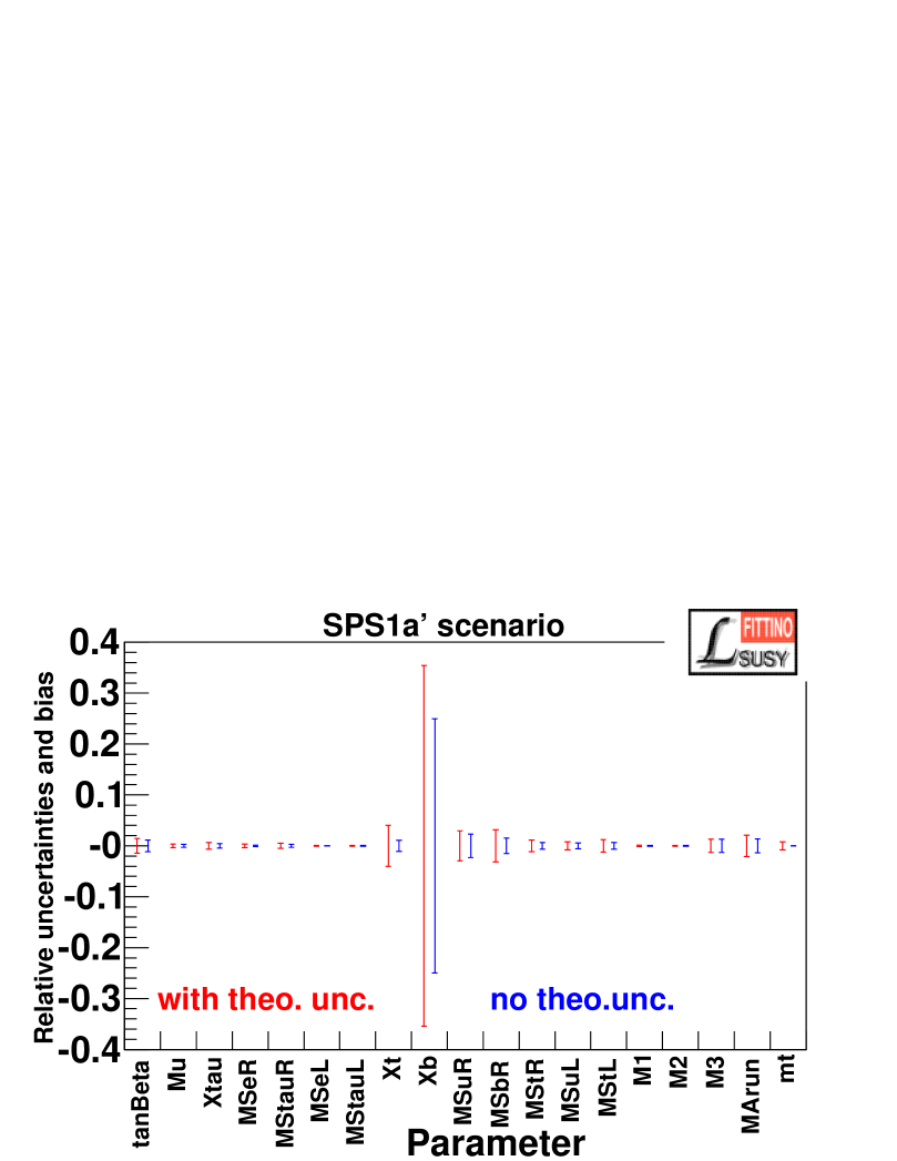
Figure 1: Relative uncertainties of the parameter measurements with (red, left error bars) and without (blue, right error bars) theoretical uncertainties.

As shown in Table 1 all parameters are perfectly reconstructed at their input values. Due to the fact that the input observables are unsmeared in this fit, the final $\chi^{2}$ is close to zero at $\chi^{2}=2.1\times 10^{-5}$.

4.1 Extraction of the Fit Uncertainties and Correlations

After a successful convergence of the simulated annealing algorithm to the input parameter values, the fit uncertainties are evaluated by carrying out many individual fits with input values randomly smeared within their uncertainty range using a Gaussian probability density. The complete covariance matrix and the correlation matrix are derived from the spread of the fitted parameter values.

For the case without and for the case with theoretical uncertainties about 1000 fits are performed. For each of those fits, the $\chi^{2}$ is minimized. For a large and complex parameter space with large correlations among the parameters this method has turned out to be more robust than a MINOS error analysis.

An example of the outcome of this procedure for the fit (with experimental uncertainties only) from Section 4 is shown in Figure 2 for the parameters $\tan\beta$, $M_{1}$, $m_{\mathrm{A}_{\mathrm{pole}}}$ and $X_{\text{b}}$ for the $\sim$1000 independent fits. All distributions apart from $m_{\mathrm{A}_{\mathrm{pole}}}$ and $X_{\text{b}}$ agree well with Gaussians.

The difference of the RMS of the parameter distribution and the width of a Gaussian fitted to the distribution (normalized to the Gaussian width) is shown in Tab. 2 for the 19 parameters. The distributions showing the largest disagreement are $m_{\mathrm{A}_{\mathrm{pole}}}$ and $X_{\text{b}}$, indicating that a parabolic error assumption for these parameters is not completely correct.

The parameter uncertainties extracted from the fit value distributions are shown in Tab. 1, while the corresponding correlation matrix is displayed in Tab. 7 and 8. Additionally, a graphical representation of the relative uncertainties of the individual parameters, both with and without theoretical uncertainties, is given in Figure 1.

Parameter	$(\text{RMS}-\sigma)/\sigma$	Parameter	$(\text{RMS}-\sigma)/\sigma$
$\tan\beta$	$0.01$	$M_{\tilde{b}_{R}}$	$0.07$
$\mu$	$0.06$	$M_{\tilde{t}_{R}}$	$0.02$
$X_{\tau}$	$0.03$	$M_{\tilde{q}_{L}}$	$0.01$
$M_{\tilde{e}_{R}}$	$0.02$	$M_{\tilde{t}_{L}}$	$0.04$
$M_{\tilde{\tau}_{R}}$	$0.00$	$M_{1}$	$0.01$
$M_{\tilde{e}_{L}}$	$0.02$	$M_{2}$	$-0.01$
$M_{\tilde{\tau}_{L}}$	$0.01$	$M_{3}$	$0.04$
$X_{\text{t}}$	$0.03$	$m_{\text{A}_{\text{run}}}$	$0.14$
$X_{\text{b}}$	$0.17$	$m_{\text{t}}$	$0.01$
$M_{\tilde{q}_{R}}$	$0.04$

Table 2: Comparison of the RMS and the Gaussian width $\sigma$ fitted to the parameter distributions.

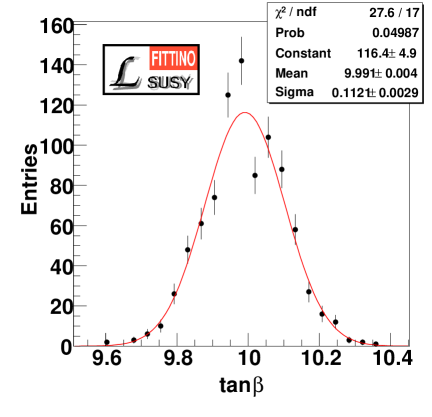
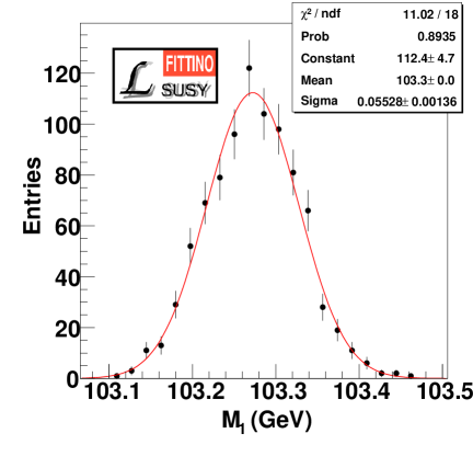
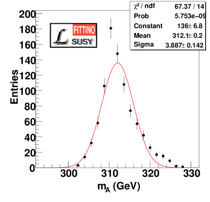
Figure 2: Examples of the toy fit value distributions for $\sim$1000 independent fits with observables smeared within their uncertainties.

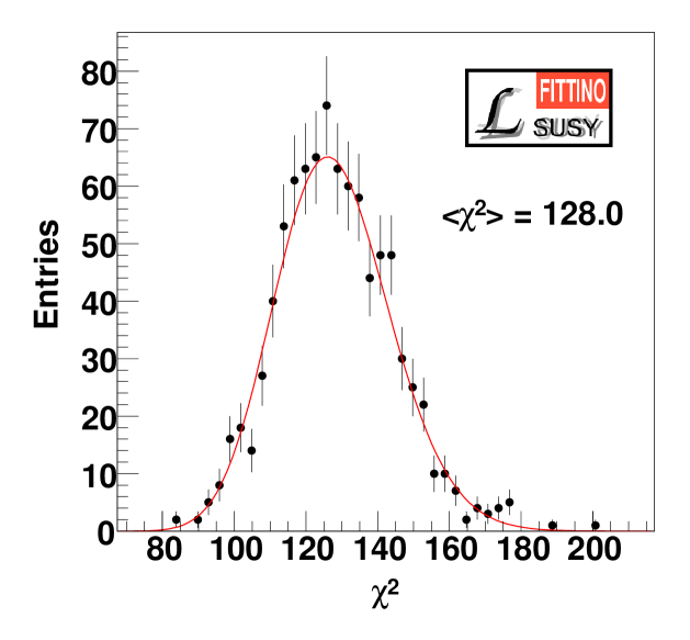
Figure 3: $\chi^{2}$ distribution for $\sim$1000 independent fits with observables smeared within their uncertainties. The mean $\chi^{2}$ from a $\chi^{2}$ function fitted to the observed distribution of 128.0 agrees with the expectation of 129.0 $\pm$ 0.7.

Figure 3 shows the distribution of the $\chi^{2}$ values for these $\sim$1000 independent fits for the case without theoretical uncertainties. The mean $\chi^{2}$ obtained from a fit of the $\chi^{2}$ distribution to the observed distribution is 128.0, in agreement with the expectation of 129.0 $\pm$ 0.7. This shows that the fits converge well to the true minimum of the $\chi^{2}$ surface for the smeared observables, implying that the uncertainties extracted from the toy fit value distributions are correct.

4.2 Interpretation of the Fit Results

Most parameters are reconstructed to a precision better than or around 1 %. For the U(1) gaugino mass parameter $M_{1}$, an accuracy below the per mil level is achieved for the fit including experimental uncertainties only. But its precision is worse by more than a factor of 2 once theoretical uncertainties are included. The uncertainties on other parameters increase by up to a factor of 3.3 if theoretical uncertainties are taken into account, such as $M_{\tilde{\text{e}}_{R}}$. In order to fully benefit from the precision data provided in particular by the ILC, more precise calculations would be beneficial.

The least constrained variables are the mixing parameters. Especially $X_{\text{b}}$ has only small influence on the Higgs sector and the sbottom masses, resulting in a relative precision of only 25 % (corresponding to 130 % relative uncertainty for $A_{\text{b}}$). The situation is better for $X_{\tau}$ and $X_{\text{t}}$. The high precision in the chargino and slepton sector as well as the occurrence of the decay channel $\text{H}^{+}\rightarrow\tilde{\nu}_{\tau_{L}}\tilde{\tau}_{1}^{+}$ allows to determine $X_{\tau}$ to an accurary of less than 0.5 % (corresponds to 9 % for $A_{\tau}$). The achieved relative precision of 1 % for $X_{\text{t}}$ (1 % for $A_{\text{t}}$) is possible due to the large mass splitting in the stop sector and its influence on the Higgs sector. Searching for sensitive observables to constrain the mixing parameters to a larger extent is important to improve their precisions.

The benefit of a global fit is that the full correlation matrix of all parameters is available (see Appendix B). As expected correlations within sectors can be strong. The parameters of the gaugino sector $\tan\beta$, $\mu$, $M_{1}$ and $M_{2}$, for example, reveal correlations up to 69 %. But even between different sectors the correlations cannot be neglected. One example is $M_{\tilde{\text{q}}_{R}}$ from the squark sector whose correlation coefficient with $M_{\tilde{\text{e}}_{R}}$ from slepton sector amounts to $-0.79$. Even the relatively robust gaugino sector is affected by such inter-sector correlations. $M_{2}$, for example, has a correlation of 20 % with $M_{\tilde{\text{q}}_{L}}$ from the sfermion sector. This underlines the importance of fitting all SUSY parameters simultaneously. Neglecting these inter-sector correlations causes incorrect fit uncertainties in fits restricted to specific sectors.

4.3 Fits in Subspaces

This section is devoted to a check of the influence of restricted fits on the precision of the reconstructed parameters and their uncertainties. It might be interesting to study the possibility to extract limited information on the SUSY parameters in a certain subspace only, because the input described in Section 3.2 will not be completely available at the beginning of ILC running at lower energies. Therefore fits with inputs restricted to the low-energy running phase of ILC have been performed. But this entails fixing parameters which cannot be determined with the low-energy data. The following excerpt of observables from Section 3.2 has been used for the fit:

• All SM observables.

• All mass measurements in the gaugino and slepton sector from ILC running at $\sqrt{s}=500$ GeV.

• All chargino, neutralino and $\tilde{e}$ cross-section times branching fraction measurements at $\sqrt{s}=400$ GeV and $\sqrt{s}=500$ GeV.

No Higgs sector parameters and observables are used in the fit, since they have large dependencies on squark sector parameters such as $X_{\text{t}}$ and $M_{\tilde{t}}$.

The fixed and fitted parameters are listed in Table 3. All fixed parameters are set to the correct values in a first fit. As shown in Table 3 the central values of the fit reproduce the correct parameter values. In a second step the fit is performed with all fixed parameters set to modified values. The chosen numbers are estimates in a situation where the strongly interacting sector has not been precisely measured yet. The quality of the fit results for this second fit depends on the chosen set of fixed and fitted parameters.

Parameter	“True” value	Fit with correctly	Fit with incorrectly	Uncertainty
		fixed parameters	fixed parameters
Fixed parameters
$X_{\text{t}}$	$-565.7\;\text{GeV}$	$-565.7\;\text{GeV}$	$-30.0\;\text{GeV}$	fixed
$X_{\text{b}}$	$-4934.8\;\text{GeV}$	$-4934.8\;\text{GeV}$	$-4000.0\;\text{GeV}$	fixed
$M_{\tilde{q}_{R}}$	$501.6\;\text{GeV}$	$501.6\;\text{GeV}$	$600.0\;\text{GeV}$	fixed
$M_{\tilde{b}_{R}}$	$497.4\;\text{GeV}$	$497.4\;\text{GeV}$	$600.0\;\text{GeV}$	fixed
$M_{\tilde{t}_{R}}$	$503.9\;\text{GeV}$	$503.9\;\text{GeV}$	$500.0\;\text{GeV}$	fixed
$M_{\tilde{q}_{L}}$	$523.2\;\text{GeV}$	$523.2\;\text{GeV}$	$500.0\;\text{GeV}$	fixed
$M_{\tilde{t}_{L}}$	$467.7\;\text{GeV}$	$467.7\;\text{GeV}$	$500.0\;\text{GeV}$	fixed
$M_{3}$	$568.9\;\text{GeV}$	$568.9\;\text{GeV}$	$700.0\;\text{GeV}$	fixed
$m_{\text{A}_{\text{run}}}$	$312.0\;\text{GeV}$	$312.0\;\text{GeV}$	$400.0\;\text{GeV}$	fixed
$m_{\text{t}}$	$178.0\;\text{GeV}$	$178.0\;\text{GeV}$	$178.0\;\text{GeV}$	fixed
Fitted parameters
$\tan\beta$	$10.00$	$10.00$	$11.1$	$0.47$
$\mu$	$400.39\;\text{GeV}$	$400.388\;\text{GeV}$	$388.3\;\text{GeV}$	$3.1\;\text{GeV}$
$X_{\tau}$	$-4449.2\;\text{GeV}$	$-4449.2\;\text{GeV}$	$-4447.8\;\text{GeV}$	$37.2\;\text{GeV}$
$M_{\tilde{e}_{R}}$	$115.60\;\text{GeV}$	$115.602\;\text{GeV}$	$113.74\;\text{GeV}$	$0.06\;\text{GeV}$
$M_{\tilde{\tau}_{R}}$	$109.89\;\text{GeV}$	$109.89\;\text{GeV}$	$107.77\;\text{GeV}$	$0.48\;\text{GeV}$
$M_{\tilde{e}_{L}}$	$181.30\;\text{GeV}$	$181.304\;\text{GeV}$	$181.76\;\text{GeV}$	$0.04\;\text{GeV}$
$M_{\tilde{\tau}_{L}}$	$179.54\;\text{GeV}$	$179.54\;\text{GeV}$	$179.99\;\text{GeV}$	$0.14\;\text{GeV}$
$M_{1}$	$103.271\;\text{GeV}$	$103.271\;\text{GeV}$	$103.11\;\text{GeV}$	$0.05\;\text{GeV}$
$M_{2}$	$193.446\;\text{GeV}$	$193.445\;\text{GeV}$	$193.49\;\text{GeV}$	$0.12\;\text{GeV}$
$\chi^{2}$		$1.8\times 10^{-5}$	$5.89$

Table 3: Fittino fits of a parameter subspace using inputs from the low-energy running of ILC only.

This test shows that subspace fits can provide results of the correct order of magnitude. Subspace fits are justified at the beginning of the exploration of SUSY phenomena where experimental uncertainties are large and only limited data is available for SUSY parameter analysis. Depending on the chosen set of fixed and fitted parameters, subspace fits might yield parameter values whose biases are several times as large as their uncertainties obtained from the fit. This unfortunate feature is a consequence of neglected correlations. The errors obtained from subsector fits do not express a probability to find the true parameter values within the uncertainty range. Uncovering these shifts by looking at the $\chi^{2}$ of the fit is unlikely in reality since a degradation of $\Delta\chi^{2}=5.89$, which is the largest $\chi^{2}$ enhancement observed in above fits, might still yield a reasonable $\chi^{2}$ value for the fit with its 85 degrees of freedom. In any case, as this example shows, a precision determination of the SUSY Lagrangian parameters requires a comprehensive global fit using inputs from all sectors of the theory and fitting parameters from all sectors of the theory.

5 Extrapolation to High Energy Scales

As soon as the complete set of parameters is known at the electroweak scale, they can be extrapolated to high energy scales to test ideas concerning SUSY breaking or grand unification within the bottom-up approach [7]. In this way one exploits the experimental information to the maximum extent possible without any assumptions on the structure of the high scale theory except that there are no new particles between the electroweak scale and the high scale.

Figure 4: Running of a) the gaugino mass parameters, b) first generation scalar mass parameters and $M^{2}_{H_{2}}$ and c) third generation scalar mass parameters and $M^{2}_{H_{1}}$ in SPS1a^′. Full bands: only experimental errors are taken into account; dashed lines: today’s theoretical errors are taken into account as a conservative estimate.

The parameters at the high energy are related to the electroweak scale parameters by renormalization group equations (RGEs). Here we use two-loop RGEs for the evolution [23]. The evolution of the parameters from the electroweak scale to the GUT scale are shown in Fig. 4 where the GUT scale is defined as the scale where the $SU(2)$ gauge coupling $g_{2}$ coincides with $U(1)$ gauge coupling $g_{1}$ (using the proper normalisation $g_{1}=\sqrt{5/3}g^{\prime}$) and the value for the electroweak scale is given by $\sqrt{m_{\tilde{t}_{1}}m_{\tilde{t}_{2}}}$. The latter value is motivated by the expectation that at this scale the effect of missing higher order corrections in the calculation of $m_{\text{h}}$, which is most probably the most precisely measured mass, is minimized.

In Fig. 4 a the evolution for the gaugino parameters $M^{-1}_{i}$ is presented. They are clearly under excellent control allowing for precise tests concerning their unification at $M_{GUT}$. Note, that their ’unification point’ is in principle independent of the one for the gauge couplings allowing for a cross check if both sets of parameters indeed meet at the same point.

In Fig. 4 b and c the running of the scalar mass parameters are shown. The slepton mass parameters are under excellent control whereas the squark and the Higgs mass parameters are signifcantly worse. Part of this difference can be traced back to the structure of the RGEs as explained in detail in the second paper of [7]. In addition the analysis used here does not coincide with ones presented in [7] and [35]: In [7] and [35] it has been assumed that all $A$ parameters meet within 1-sigma as up to now no good proposal exists for a precise measurement of $A_{b}$. As we did not use this assumption in this study we find significantly larger errors for the third generation squark mass parameters and the Higgs parameters. Using this assumption or, equivalently, having tools at hand which allow for a better determination of $A_{\text{b}}$, the error bands get significantly reduced as can be seen in Fig. 5 where we show the running of the same parameters as in Fig. 4 c assuming that $A_{\text{b}}$ is known within 50 % at the electroweak scale.

Figure 5: Running of third generation scalar mass parameters and $M^{2}_{H_{1}}$ in SPS1a^′ assuming that $A_{\text{b}}$ is known with an ’accuracy’ of 50%.

In Fig. 4 we also show the case that today’s theoretical uncertainties are taken into account (dashed lines). In case of the gaugino mass parameters the effect is so small that it cannot be seen in the plot (see also Tab. 1). Note that the smallness of the theoretical uncertainty on the gluino mass is due to the fact that the squarks have a similar mass. It gets larger if there is a significant hierarchy between these particles, e. g. in focus point scenarios. One sees that the main effect is on the parameters of the third generation sfermions and the Higgs mass parameters. The main reason for this is that the error on $X_{\text{b}}$ and $M_{\tilde{\text{b}}_{R}}$ get considerably larger once the theoretical uncertainties are taken into account. This figure clearly shows that there is a strong need to further increase accuracies of the theoretical predictions.

6 Fit Within mSUGRA Framework

Instead of determining the full spectrum of the general low-energy Lagrangian parameters and inferring the high-scale mechanisms from them, the parameters of a more restrictive high-scale scenario can be fitted directly to the observables. This section presents an example for the mSUGRA scenario SPS1a’, using the same set of observables as described in Section 3.2. The parameters of the scenario are $\tan\beta$, $M_{0}$, $M_{1/2}$, $A_{0}$ and $\text{sign}(\mu)$. The latter has been fixed to 1 for this exercise.

Since there are only four continuous parameters, the fit converges without complex fitting techniques and the uncertainty determination is stable. The fit results for the simulated LHC+ILC measurements from Section 4 and observables set to the exact prediction of the mSUGRA model are given in Table 4, along with results for a fit just using the LHC observables in the fit. As an additional LHC measurement, the ratio of Higgs couplings as simulated in [36] has been used. For the LHC$+$ILC measurements, due to the much more constrained theoretical parameter space, the precision on the parameters is much better than for the general low-energy model (see Table 1). For the same reason, the LHC alone is able to perform well constrained parameter measurements with uncertainties typically one to two orders of magnitude larger than in the case of the combination of both.

	SPS1a’ value	Fitted value	$\Delta_{\text{LHC$+$ILC}}$	$\Delta_{\text{LHC only}}$
$\tan\beta$	$10.000$	$10.000$	$0.036$	$1.3$
$M_{0}$ (GeV)	$70.000$	$70.000$	$0.070$	$1.4$
$M_{1/2}$ (GeV)	$250.000$	$250.000$	$0.065$	$1.0$
$A_{0}$ (GeV)	$-300.0$	$-300.0$	$2.5$	$16.6$

Table 4: Fit results for fits within mSUGRA scenario. The meanings of the columns are (starting from the left): SPS1a’ values, the fitted mSUGRA parameters, parameter uncertainties for a fit to LHC$+$ILC observables and parameter uncertainties for a fit to “LHC only” observables. In both cases theoretical uncertainties are not included.

An important test is, however, to determine how well the experimental results can be used to determine deviations from a specific high-scale model such as mSUGRA. Therefore the mSUGRA high-energy parameters have been fitted to the observables from the SPS1a’ inspired scenario used in Section 3, which is only slightly modified to obtain exact unification in the first two generations of squarks and sleptions. For this case, the total $\chi^{2}$s from the two fits indicate that the LHC$+$ILC measurements are precise enough to discriminate the modified scenario from exact mSUGRA ($\chi^{2}=3600$, 144 n.d.f.), while the LHC measurements alone do not allow this insight ($\chi^{2}=0.5$, 25 n.d.f.).

7 Conclusions

The Lagrangian parameters of the MSSM assuming universality for the first and second generation and real parameters but without assumptions on the SUSY breaking mechanism are correctly reconstructed without usage of a priori information. This has been achieved using precision measurements at the LHC and ILC as input to a global fit exploiting the techniques implemented in the program Fittino.

Most of the Lagrangian parameters can be determined to a precision around the percent level. For some parameters an accuracy of better than 1 per mil is achievable if theoretical uncertainties are neglected. As a (very) conservative estimate we have re-done the fit using today’s theoretical uncertainties. As expected it turns out that they can significantly deteriorate the precision of the Lagrangian parameter determination. More work is needed to improve the accurary of theoretical predictions in order to fully benefit from the experimental precision. The only parameter which cannot be strongly constrained by the observables used in the presented fit is $X_{\text{b}}$ resulting in a precision of only 25 % for this parameter which translates into an uncertainty of 130 % on $A_{\text{b}}$.

The strong (inter-sector) correlations between the fitted parameters underline the importance of performing a global fit including all sectors of the theory. As shown, fits in parameter subspaces can lead to significant biases and wrong uncertainty estimates.

The fitted parameters at the electroweak scale have been extrapolated to high scales using the bottom-up approach taking into account all correlations between the errors. We have found that the gaugino sector as well as the slepton sector can be reconstructed rather precisely allowing for stringent tests of the underlying model in these sectors. The accuracy deteriorates considerably for squark mass parameters and the Higgs mass parameters. The results clearly show how far the squark mass parameters can deviate from the universality assumption indicated by the measurements in the slepton sector. We have also performed a top-down fit of the high-energy mSUGRA parameters to combined LHC$+$ILC observables. Here we have found that they are very sensitive to even tiny deviations from the mSUGRA hypothesis. The discriminative power of “LHC only” inputs is significantly weaker.

Appendix A List of Input Observables to the SPS1a’ Inspired Fit

Observable	Value	Exp. uncertainty
$m_{\text{W}}$	$80.3371\;\text{GeV}$	$0.039\;\text{GeV}$
$m_{\text{Z}}$	$91.1187\;\text{GeV}$	$0.0021\;\text{GeV}$
$m_{\text{t}}$	$178.0\;\text{GeV}$	$0.05\;\text{GeV}$
$m_{\text{h}}$	$112.888\;\text{GeV}$	$0.05\;\text{GeV}$
$m_{\text{A}_{\text{pole}}}$	$374.228\;\text{GeV}$	$1.3\;\text{GeV}$
$m_{\text{H}}$	$374.464\;\text{GeV}$	$1.3\;\text{GeV}$
$m_{\text{H}^{\pm}}$	$383.131\;\text{GeV}$	$1.1\;\text{GeV}$
$m_{\tilde{q}_{L}}$	$561.539\;\text{GeV}$	$9.8\;\text{GeV}$
$m_{\tilde{q}_{R}}$	$543.35\;\text{GeV}$	$11.0\;\text{GeV}$
$m_{\tilde{b}_{1}}$	$502.059\;\text{GeV}$	$5.7\;\text{GeV}$
$m_{\tilde{b}_{2}}$	$541.81\;\text{GeV}$	$6.2\;\text{GeV}$
$m_{\tilde{t}_{1}}$	$365.819\;\text{GeV}$	$2.0\;\text{GeV}$
$m_{\tilde{e}_{L}}$	$190.209\;\text{GeV}$	$0.2\;\text{GeV}$
$m_{\tilde{e}_{R}}$	$124.883\;\text{GeV}$	$0.05\;\text{GeV}$
$m_{\tilde{\mu}_{L}}$	$190.237\;\text{GeV}$	$0.5\;\text{GeV}$
$m_{\tilde{\mu}_{R}}$	$124.837\;\text{GeV}$	$0.2\;\text{GeV}$
$m_{\tilde{\tau}_{1}}$	$107.292\;\text{GeV}$	$0.3\;\text{GeV}$
$m_{\tilde{\tau}_{2}}$	$195.290\;\text{GeV}$	$1.1\;\text{GeV}$
$m_{\tilde{\text{g}}}$	$603.639\;\text{GeV}$	$6.4\;\text{GeV}$
$m_{\tilde{\chi}^{0}_{1}}$	$97.7662\;\text{GeV}$	$0.05\;\text{GeV}$
$m_{\tilde{\chi}^{0}_{2}}$	$184.345\;\text{GeV}$	$0.08\;\text{GeV}$
$m_{\tilde{\chi}^{0}_{3}}$	$404.134\;\text{GeV}$	$4.0\;\text{GeV}$
$m_{\tilde{\chi}^{0}_{4}}$	$417.037\;\text{GeV}$	$2.3\;\text{GeV}$
$m_{\tilde{\chi}^{\pm}_{1}}$	$184.132\;\text{GeV}$	$0.55\;\text{GeV}$
$m_{\tilde{\chi}^{\pm}_{2}}$	$418.495\;\text{GeV}$	$3.0\;\text{GeV}$
Edge 3 with $m_{\tilde{\chi}^{0}_{1}}$, $m_{\tilde{q}_{L}}$, $m_{\tilde{\chi}^{0}_{2}}$	$449.679\;\text{GeV}$	$4.9\;\text{GeV}$
Edge 3 with $m_{\tilde{\mu}_{R}}$, $m_{\tilde{q}_{L}}$, $m_{\tilde{\chi}^{0}_{2}}$	$390.285\;\text{GeV}$	$3.35\;\text{GeV}$
Edge 4 with $m_{\tilde{\chi}^{0}_{1}}$, $m_{\tilde{\chi}^{0}_{2}}$, $m_{\tilde{\mu}_{R}}$, $m_{\tilde{q}_{L}}$	$329.831\;\text{GeV}$	$4.2\;\text{GeV}$
Edge 5 with $m_{\tilde{\chi}^{0}_{1}}$, $m_{\tilde{\chi}^{0}_{2}}$, $m_{\tilde{\mu}_{R}}$, $m_{\tilde{q}_{L}}$	$218.529\;\text{GeV}$	$3.44\;\text{GeV}$

Table 5: Simulated measurements at LHC and at ILC running at 400 GeV, 500 GeV and 1 TeV center-of-mass energy. The values of the observables are taken from the prediction of SPheno version 2.2.2 for the SPS1a’ inspired scenario. The experimental uncertainties on the masses are taken from [15]. The definition of the edge numbers can be found in [9].

Observable	Theor. uncertainty
$m_{\text{t}}$	$0.1\;\text{GeV}$
$m_{\text{h}}$	$1.3\;\text{GeV}$
$m_{\text{A}_{\text{pole}}}$	$0.7\;\text{GeV}$
$m_{\text{H}}$	$0.7\;\text{GeV}$
$m_{\text{H}^{\pm}}$	$0.7\;\text{GeV}$
$m_{\tilde{q}_{L}}$	$10.2\;\text{GeV}$
$m_{\tilde{q}_{R}}$	$9.4\;\text{GeV}$
$m_{\tilde{b}_{1}}$	$8.0\;\text{GeV}$
$m_{\tilde{b}_{2}}$	$10.2\;\text{GeV}$
$m_{\tilde{t}_{1}}$	$5.4\;\text{GeV}$
$m_{\tilde{e}_{L}}$	$0.4\;\text{GeV}$
$m_{\tilde{e}_{R}}$	$1.2\;\text{GeV}$
$m_{\tilde{\mu}_{L}}$	$0.4\;\text{GeV}$
$m_{\tilde{\mu}_{R}}$	$1.2\;\text{GeV}$
$m_{\tilde{\tau}_{1}}$	$0.5\;\text{GeV}$
$m_{\tilde{\tau}_{2}}$	$0.5\;\text{GeV}$
$m_{\tilde{\text{g}}}$	$1.4\;\text{GeV}$
$m_{\tilde{\chi}^{0}_{1}}$	$0.4\;\text{GeV}$
$m_{\tilde{\chi}^{0}_{2}}$	$1.2\;\text{GeV}$
$m_{\tilde{\chi}^{0}_{3}}$	$1.2\;\text{GeV}$
$m_{\tilde{\chi}^{0}_{4}}$	$1.2\;\text{GeV}$
$m_{\tilde{\chi}^{\pm}_{1}}$	$1.3\;\text{GeV}$
$m_{\tilde{\chi}^{\pm}_{2}}$	$1.3\;\text{GeV}$
Edge 3 with $m_{\tilde{\chi}^{0}_{1}}$, $m_{\tilde{q}_{L}}$, $m_{\tilde{\chi}^{0}_{2}}$	$4.5\;\text{GeV}$
Edge 3 with $m_{\tilde{\mu}_{R}}$, $m_{\tilde{q}_{L}}$, $m_{\tilde{\chi}^{0}_{2}}$	$3.9\;\text{GeV}$
Edge 4 with $m_{\tilde{\chi}^{0}_{1}}$, $m_{\tilde{\chi}^{0}_{2}}$, $m_{\tilde{\mu}_{R}}$, $m_{\tilde{q}_{L}}$	$3.3\;\text{GeV}$
Edge 5 with $m_{\tilde{\chi}^{0}_{1}}$, $m_{\tilde{\chi}^{0}_{2}}$, $m_{\tilde{\mu}_{R}}$, $m_{\tilde{q}_{L}}$	$2.19\;\text{GeV}$

Table 6: Theoretical uncertainties on the masses (taken from [17]) and the induced ones on the edge variables.

Appendix B Correlation Matrix of the SPS1a’ Inspired Fit

Table 7 and 8 show the full correlation matrix from the fit for the SPS1a’ inspired scenario described in Section 3.

Parameter	$\tan\beta$	$\mu$	$X_{\tau}$	$M_{\tilde{e}_{R}}$	$M_{\tilde{\tau}_{R}}$	$M_{\tilde{e}_{L}}$	$M_{\tilde{\tau}_{L}}$	$X_{\text{t}}$	$X_{\text{b}}$	$M_{\tilde{q}_{R}}$
$\tan\beta$	$1.000$	$-0.509$	$-0.238$	$0.042$	$0.032$	$-0.125$	$-0.321$	$0.030$	$-0.569$	$0.033$
$\mu$	$-0.509$	$1.000$	$0.014$	$-0.038$	$-0.028$	$0.303$	$0.308$	$-0.064$	$0.151$	$0.031$
$X_{\tau}$	$-0.238$	$0.014$	$1.000$	$0.055$	$-0.431$	$-0.076$	$0.225$	$-0.137$	$-0.091$	$-0.058$
$M_{\tilde{e}_{R}}$	$0.042$	$-0.038$	$0.055$	$1.000$	$0.369$	$-0.631$	$-0.329$	$0.026$	$-0.109$	$-0.793$
$M_{\tilde{\tau}_{R}}$	$0.032$	$-0.028$	$-0.431$	$0.369$	$1.000$	$-0.254$	$-0.339$	$0.062$	$0.074$	$-0.362$
$M_{\tilde{e}_{L}}$	$-0.125$	$0.303$	$-0.076$	$-0.631$	$-0.254$	$1.000$	$0.368$	$-0.048$	$0.112$	$0.557$
$M_{\tilde{\tau}_{L}}$	$-0.321$	$0.308$	$0.225$	$-0.329$	$-0.339$	$0.368$	$1.000$	$-0.023$	$0.121$	$0.320$
$X_{\text{t}}$	$0.030$	$-0.064$	$-0.137$	$0.026$	$0.062$	$-0.048$	$-0.023$	$1.000$	$-0.360$	$0.097$
$X_{\text{b}}$	$-0.569$	$0.151$	$-0.091$	$-0.109$	$0.074$	$0.112$	$0.121$	$-0.360$	$1.000$	$-0.090$
$M_{\tilde{q}_{R}}$	$0.033$	$0.031$	$-0.058$	$-0.793$	$-0.362$	$0.557$	$0.320$	$0.097$	$-0.090$	$1.000$
$M_{\tilde{b}_{R}}$	$-0.049$	$0.037$	$-0.016$	$0.193$	$0.080$	$-0.133$	$-0.011$	$0.076$	$0.004$	$0.091$
$M_{\tilde{t}_{R}}$	$-0.166$	$0.125$	$-0.011$	$-0.335$	$-0.141$	$0.327$	$0.210$	$-0.371$	$0.307$	$0.082$
$M_{\tilde{q}_{L}}$	$-0.065$	$0.025$	$-0.035$	$0.192$	$0.069$	$-0.084$	$-0.001$	$0.144$	$-0.014$	$0.076$
$M_{\tilde{t}_{L}}$	$-0.005$	$-0.094$	$0.054$	$0.109$	$0.001$	$-0.138$	$-0.066$	$-0.270$	$0.092$	$0.070$
$M_{1}$	$-0.147$	$-0.263$	$0.118$	$0.169$	$0.051$	$-0.177$	$0.032$	$0.044$	$0.130$	$-0.244$
$M_{2}$	$0.229$	$-0.694$	$-0.299$	$-0.047$	$0.062$	$0.087$	$0.024$	$0.128$	$0.042$	$-0.058$
$M_{3}$	$0.044$	$0.003$	$-0.036$	$0.078$	$0.065$	$-0.046$	$-0.061$	$0.076$	$-0.070$	$-0.180$
$m_{\text{A}_{\text{run}}}$	$-0.594$	$0.143$	$-0.048$	$-0.108$	$0.056$	$0.110$	$0.130$	$-0.223$	$0.972$	$-0.076$
$m_{\text{t}}$	$-0.004$	$-0.013$	$0.004$	$-0.005$	$0.018$	$-0.018$	$0.039$	$0.186$	$-0.029$	$0.011$

Table 7: Correlation matrix of the Fittino SPS1a’ motivated fit, part I.

Parameter	$M_{\tilde{b}_{R}}$	$M_{\tilde{t}_{R}}$	$M_{\tilde{q}_{L}}$	$M_{\tilde{t}_{L}}$	$M_{1}$	$M_{2}$	$M_{3}$	$m_{\text{A}_{\text{run}}}$	$m_{\text{t}}$
$\tan\beta$	$-0.049$	$-0.166$	$-0.065$	$-0.005$	$-0.147$	$0.229$	$0.044$	$-0.594$	$-0.004$
$\mu$	$0.037$	$0.125$	$0.025$	$-0.094$	$-0.263$	$-0.694$	$0.003$	$0.143$	$-0.013$
$X_{\tau}$	$-0.016$	$-0.011$	$-0.035$	$0.054$	$0.118$	$-0.299$	$-0.036$	$-0.048$	$0.004$
$M_{\tilde{e}_{R}}$	$0.193$	$-0.335$	$0.192$	$0.109$	$0.169$	$-0.047$	$0.078$	$-0.108$	$-0.005$
$M_{\tilde{\tau}_{R}}$	$0.080$	$-0.141$	$0.069$	$0.001$	$0.051$	$0.062$	$0.065$	$0.056$	$0.018$
$M_{\tilde{e}_{L}}$	$-0.133$	$0.327$	$-0.084$	$-0.138$	$-0.177$	$0.087$	$-0.046$	$0.110$	$-0.018$
$M_{\tilde{\tau}_{L}}$	$-0.011$	$0.210$	$-0.001$	$-0.066$	$0.032$	$0.024$	$-0.061$	$0.130$	$0.039$
$X_{\text{t}}$	$0.076$	$-0.371$	$0.144$	$-0.270$	$0.044$	$0.128$	$0.076$	$-0.223$	$0.186$
$X_{\text{b}}$	$0.004$	$0.307$	$-0.014$	$0.092$	$0.130$	$0.042$	$-0.070$	$0.972$	$-0.029$
$M_{\tilde{q}_{R}}$	$0.091$	$0.082$	$0.076$	$0.070$	$-0.244$	$-0.058$	$-0.180$	$-0.076$	$0.011$
$M_{\tilde{b}_{R}}$	$1.000$	$0.009$	$-0.017$	$-0.077$	$-0.034$	$0.024$	$-0.105$	$0.026$	$0.012$
$M_{\tilde{t}_{R}}$	$0.009$	$1.000$	$-0.036$	$-0.428$	$-0.048$	$0.045$	$-0.236$	$0.249$	$-0.063$
$M_{\tilde{q}_{L}}$	$-0.017$	$-0.036$	$1.000$	$0.057$	$0.006$	$-0.200$	$-0.275$	$0.011$	$0.017$
$M_{\tilde{t}_{L}}$	$-0.077$	$-0.428$	$0.057$	$1.000$	$-0.002$	$-0.140$	$-0.225$	$0.106$	$-0.081$
$M_{1}$	$-0.034$	$-0.048$	$0.006$	$-0.002$	$1.000$	$0.293$	$0.055$	$0.141$	$-0.060$
$M_{2}$	$0.024$	$0.045$	$-0.200$	$-0.140$	$0.293$	$1.000$	$0.109$	$0.040$	$-0.005$
$M_{3}$	$-0.105$	$-0.236$	$-0.275$	$-0.225$	$0.055$	$0.109$	$1.000$	$-0.086$	$0.008$
$m_{\text{A}_{\text{run}}}$	$0.026$	$0.249$	$0.011$	$0.106$	$0.141$	$0.040$	$-0.086$	$1.000$	$-0.008$
$m_{\text{t}}$	$0.012$	$-0.063$	$0.017$	$-0.081$	$-0.060$	$-0.005$	$0.008$	$-0.008$	$1.000$

Table 8: Correlation matrix of the Fittino SPS1a’ motivated fit, part II.

References

- [1] J. Wess and B. Zumino, Nucl. Phys. B 70(1974) 39.
-
[2]
ATLAS Coll., Technical Design Report, CERN/LHCC/99-15 (1999);
CMS Coll., Technical Proposal, CERN/LHCC/94-38 (1994);
J. G. Branson, D. Denegri, I. Hinchliffe, F. Gianotti, F. E. Paige and P. Sphicas [ATLAS and CMS Collaborations], Eur. Phys. J. C direct4 (2002) N1; -
[3]
J. A. Aguilar-Saavedra et al. [ECFA/DESY LC Physics Working Group Collaboration], [arXiv:hep-ph/0106315];
T. Abe et al. [American Linear Collider Working Group Collaboration], in Proc. of Snowmass 2001, ed. N. Graf, [arXiv:hep-ex/0106055];
K. Abe et al. [ACFA Linear Collider Working Group Coll.], [arXiv:hep-ph/0109166]; see: http://lcdev.kek.jp/RMdraft/ . - [4] A. H. Chamseddine, R. Arnowitt and P. Nath, Phys. Rev. Lett. 49 (1982) 970;
- [5] ATLAS Technical Design Report, CERN/LHCC/99-15, ATLAS TDR 15 (1999); CMS Technical Proposal, CERN/LHCC/94-38 (1994); B. C. Allanach, S. Kraml and W. Porod, JHEP 0303, 016 (2003) [arXiv:hep-ph/0302102]; G. Polesello and D. R. Tovey, JHEP 0405 (2004) 071 [arXiv:hep-ph/0403047].
- [6] see e. g. H. P. Nilles, Phys. Rept. 110 (1984) 1.
- [7] G. A. Blair, W. Porod and P. M. Zerwas, Eur. Phys. J. C 27 (2003) 263 [arXiv:hep-ph/0210058] ; Phys. Rev. D 63 (2001) 017703 [arXiv:hep-ph/0007107].
- [8] F. James, M. Roos, Comp. Phys. Commun. 10 (1975) 343.
- [9] P. Bechtle, K. Desch, P. Wienemann, [arXiv:hep-ph/0412012], accepted by Comp. Phys. Commun.
-
[10]
E. D. Commins, S. B. Ross, D. DeMille, and B. C. Regan,
Phys. Rev. A 50(1994) 2960;
P. G. Harris et al., Phys. Rev. Lett. 82(1999) 904. - [11] S. Eidelman et al. [Particle Data Group], Phys. Lett. B 592 (2004) 1.
- [12] F. Gabbiani, E. Gabrielli, A. Masiero and L. Silvestrini, Nucl. Phys. B 477 (1996) 321 [arXiv:hep-ph/9604387].
- [13] ATLAS Coll., Technical Design Report, CERN/LHCC/99-15 (1999);
- [14] CMS Coll., Technical Proposal, CERN/LHCC/94-38 (1994);
- [15] LHC/LC Study Group, G. Weiglein et al., [arXiv:hep-ph/0410364], submitted to Phys. Rep.
- [16] W. Majerotto, arXiv:hep-ph/0209137; T. Fritzsche and W. Hollik, Nucl. Phys. Proc. Suppl. 135 (2004) 102 [arXiv:hep-ph/0407095]; W. Hollik, talk at SUSY’05, Durham, England, July 18-23, 2005, http://susy-2005.dur.ac.uk/susy05programme.html .
- [17] SPA working group, Supersymmetry Parameter Analysis: SPA Convention and Project, draft available at http://spa.desy.de/spa.
- [18] W. Porod, Comp. Phys. Commun. 153 (2003) 275.
- [19] D. M. Pierce, J. A. Bagger, K. T. Matchev and R. j. Zhang, Nucl. Phys. B 491 (1997) 3 [arXiv:hep-ph/9606211].
- [20] G. Degrassi, P. Slavich and F. Zwirner, Nucl. Phys. B 611 (2001) 403 [arXiv:hep-ph/0105096]; A. Brignole, G. Degrassi, P. Slavich and F. Zwirner, Nucl. Phys. B 631 (2002) 195 [arXiv:hep-ph/0112177]; Nucl. Phys. B 643 (2002) 79 [arXiv:hep-ph/0206101]; A. Dedes and P. Slavich, Nucl. Phys. B 657 (2003) 333 [arXiv:hep-ph/0212132]; B. C. Allanach et al.,JHEP 0409, 044 (2004) [arXiv:hep-ph/0406166].
- [21] H. Eberl, A. Bartl and W. Majerotto, Nucl. Phys. B 472 (1996) 481 [arXiv:hep-ph/9603206].
- [22] E. A. Kuraev and V. S. Fadin, Sov. J. Nucl. Phys. 41 (1985) 466 [Yad. Fiz. 41 (1985) 733].
- [23] S. P. Martin and M. T. Vaughn, Phys. Rev. D 50 (1994) 2282 [arXiv:hep-ph/9311340]; Y. Yamada, Phys. Rev. D 50 (1994) 3537 [arXiv:hep-ph/9401241]; I. Jack and D. R. T. Jones, Phys. Lett. B 333 (1994) 372 [arXiv:hep-ph/9405233].
- [24] P. Bechtle, K. Desch, P. Wienemann, Fittino, available at http://www-flc.desy.de/fittino.
- [25] R. Lafaye, T. Plehn and D. Zerwas, [arXiv:hep-ph/0404282].
- [26] A. Corona et al., ACM Transactions on Mathematical Software 13(1987) 262.
- [27] W. L. Goffe, G. D. Ferrier, and J. Rogers, Journal of Econometrics 60(1994) 65.
- [28] B. C. Allanach et al., Eur. Phys. J. C 25 (2002) 113.
- [29] G. Belanger, F. Boudjema, A. Cottrant, A. Pukhov and A. Semenov, Nucl. Phys. B 706 (2005) 411 [arXiv:hep-ph/0407218].
- [30] R.-D. Heuer, D. Miller, F. Richard, P. Zerwas, TESLA Technical Design Report, Part III: Physics at an Linear Collider, DESY, Hamburg, Germany, DESY 2001-011 and ECFA 2001-209, March 2001, arXiv:hep-ph/0106315.
- [31] A. H. Hoang, [arXiv:hep-ph/0412160].
- [32] S. Y. Choi, A. Djouadi, M. Guchait, J. Kalinowski, H. S. Song and P. M. Zerwas, Eur. Phys. J. C 14 (2000) 535 [arXiv:hep-ph/0002033].
- [33] S. Y. Choi, J. Kalinowski, G. Moortgat-Pick and P. M. Zerwas, Eur. Phys. J. C 22 (2001) 563 [Addendum-ibid. C 23 (2002) 769] [arXiv:hep-ph/0108117].
- [34] A. Freitas, W. Porod and P. M. Zerwas, [arXiv:hep-ph/0509056].
- [35] B. C. Allanach, G. A. Blair, S. Kraml, H. U. Martyn, G. Polesello, W. Porod and P. M. Zerwas, [arXiv:hep-ph/0403133].
- [36] M. Dührssen, Prospects for the measurement of Higgs boson coupling parameters in the mass range from 110 - 190 GeV/, ATLAS-PHYS-2003-030; M. Dührssen et al., Phys. Rev. D 70 (2004) 113009.