Quark–antiquark states and their radiative transitions in terms of the spectral integral equation.
II. Charmonia.

Abstract

In the precedent paper of the authors (hep-ph/0510410), the $b\bar{b}$ states were treated in the framework of the spectral integral equation, together with simultaneous calculations of radiative decays of the considered bottomonia. In the present paper, such a study is carried out for the charmonium $(c\bar{c})$ states. We reconstruct the interaction in the $c\bar{c}$-sector on the basis of data for the charmonium levels with $J^{PC}=0^{-+}$, $1^{--}$, $0^{++}$, $1^{++}$, $2^{++}$, $1^{+-}$ and radiative transitions $\psi(2S)\to\gamma\chi_{c0}(1P)$, $\gamma\chi_{c1}(1P)$, $\gamma\chi_{c2}(1P)$, $\gamma\eta_{c}(1S)$ and $\chi_{c0}(1P)$, $\chi_{c1}(1P)$, $\chi_{c2}(1P)\to\gamma J/\psi$. The $c\bar{c}$ levels and their wave functions are calculated for the radial excitations with $n\leq 6$. Also, we determine the $c\bar{c}$ component of the photon wave function using the $e^{+}e^{-}$ annihilation data: $e^{+}e^{-}\to J/\psi(3097)$, $\psi(3686)$, $\psi(3770)$, $\psi(4040)$, $\psi(4160)$, $\psi(4415)$ and perform the calculations of the partial widths of the two-photon decays for the $n=1$ states: $\eta_{c0}(1S)$, $\chi_{c0}(1P)$, $\chi_{c2}(1P)\to\gamma\gamma$, and $n=2$ states: $\eta_{c0}(2S)\to\gamma\gamma$, $\chi_{c0}(2P)$, $\chi_{c2}(2P)\to\gamma\gamma$. We discuss the status of the recently observed $c\bar{c}$ states $X(3872)$ and $Y(3941)$: according to our results, the $X(3872)$ can be either $\chi_{c1}(2P)$ or $\eta_{c2}(1D)$, while $Y(3941)$ is $\chi_{c2}(2P)$.

1 Introduction

In this paper, we continue the study initiated in [1] for the $b\bar{b}$ states in the framework of the spectral integral equation. Here the results for the $c\bar{c}$-states are presented.

In [2], the program has been formulated for the reconstruction of the quark–antiquark interaction based on our knowledge of meson levels and their radiative decays. Within this program, as a first step we have considered the bottomonia [1]. Now we present analogous results for the charmonia. In the subsequent publication, we suggest to give corresponding results for the light quark–antiquark systems.

Our study is carried out in terms of the spectral integral technique. The application of this technique to the composite quark–antiquark systems and its relation to the dispersion $N/D$-method have been discussed in [1, 2] — one may find there necessary details.

Still, let us point once again to particular properties of our approach. The quark–antiquark interaction given, the spectral integral equations provides us unambiguously with both levels and wave functions of composite systems. But if the interaction is unknown, to reconstruct it one needs to know the levels as well as their wave functions. Our knowledge of the interaction of constituent quarks (in particular, long-range interaction) is rather fragmentary, so actually the description of the composite quark–antiquark systems means the reconstruction of quark interaction. To this aim, one needs the information on the wave function of a level, and the radiative decays are precisely the source of information for the wave functions. Because of that, in our investigation of the quark–antiquark states we rely equally upon our knowledge of levels and radiative decays.

The method of calculation of the radiative transition amplitudes in terms of the double dispersion integrals was developed in a number of papers [3, 4, 5], where the important point was the representation of the transition amplitude in the form convenient for simultaneous fitting to the spectral integral equation — it was done in [6, 7].

An important information on the $c\bar{c}$-meson wave function is hidden in the two-photon meson decays: $c\bar{c}-meson\to\gamma\gamma$. For the calculation of such a type processes, the quark wave function of the photon is needed; correspondingly, the method of reconstruction of the $\gamma\to c\bar{c}$ vertices was developed in [8]. The results of calculations of the $c\bar{c}$-mesons are presented in Section 2. The known levels with $J^{PC}=0^{-+}$, $1^{--}$, $0^{++}$, $1^{++}$, $2^{++}$, $1^{+-}$ have been included in the fitting procedure, together with the widths of radiative transitions as follows: $\psi(2S)\to\gamma\chi_{c0}(1P)$, $\gamma\chi_{c1}(1P)$, $\gamma\chi_{c2}(1P)$, $\gamma\eta_{c}(1S)$ and $\chi_{c0}(1P)$, $\chi_{c1}(1P)$, $\chi_{c2}(1P)\to\gamma J/\psi$. The masses of the states have been calculated for the radial quantum numbers $n\leq 6$ and radiative transition amplitudes for the states with $n\leq 2$. Let us emphasize that we face rather significant relativistic effects in the case of excited states.

The recently observed states $X(3872)$ and $Y(3941)$ [9, 10, 11, 12] are lively discussed at present time [13, 14, 15, 16, 17, 18, 19, 20, 21, 22]. Our calculations argue that $X(3872)$ is either the excited $1^{++}$-state $\chi_{c1}(2P)$, or basic $2^{-+}$-state $\eta_{c2}(1D)$. The charmonium $Y(3941)$ state can be the radial excited $2^{++}$ state, $\chi_{c2}(2P)$.

We determine the $c\bar{c}$ component of the photon wave function using the transitions $e^{+}e^{-}\to J/\psi(3097)$, $\psi(3686)$, $\psi(3770)$, $\psi(4040)$, $\psi(4160)$, $\psi(4415)$ that allow us to calculate partial widths of the two-photon decays. We present the results for the $1S$, $1P$ states: $\eta_{c0}(2979)$, $\chi_{c0}(3415)$, $\chi_{c2}(3556)\to\gamma\gamma$, and $2S$, $2P$ states: $\eta_{c0}(3594)$, $\chi_{c0}(3849)$, $\chi_{c2}(3950)\to\gamma\gamma$. The predictions are also given for the two-photon decays $\eta_{c0},\chi_{c0}$, $\chi_{c2}\to\gamma\gamma$ of the states below $4$ GeV.

In Conclusion, we briefly summarize the results.

2 Charmonium states

We calculate the $c\bar{c}$ levels and their wave functions using two types of the $t$-channel exchanges: scalar and vector states, ($I\otimes I$) and ($\gamma_{\mu}\otimes\gamma_{\mu}$). The calculations of the $c\bar{c}$-systems have been carried out similarly to the consideration of bottomonia [1], with both retardation interaction (Solution $R(c\bar{c})$) and three variants of instantaneous interactions (Solutions $I(c\bar{c})$, $II(c\bar{c})$ and $U(c\bar{c})$). In the case of instantaneous interactions, the $t$-channel exchanges may be represented by using the potentials. In the fitting to the $c\bar{c}$ spectra, we have applied scalar and vector potentials of the type:

$$a+b\,r+c\,e^{-\mu_{c}r}+\frac{d}{r}\,e^{-\mu_{d}r}\ .$$ (1)

The presentation of these interactions in the momentum space, also with retardation effects, is given in [1].

The interaction parameters obtained in the fit are as follows (in GeV units):

Interaction Solution $$a$$

As concerns the solution $U(c\bar{c})$, we have included into calculations the scalar and vector confinement forces, with $b_{S}=-b_{V}=0.150$ GeV². The vector confinement potential is needed for the description of the light quark states ($q\bar{q}$) with large masses. In this way, solution $U(c\bar{c})$ gives us the description of data with a universal confinement potential for all flavours.

The $\alpha_{s}$ coupling, being determined by the one-gluon exchange forces, is of the same order in all solutions: $\alpha_{s}=3/4\cdot d_{V}\simeq 0.38$.

The mass of the constituent $c$-quark is taken to be $m_{c}=1.25$ GeV. This mass value is consistent with the magnitude provided by the heavy-quark effective theory [23, 24]: $1.0\leq m_{c}\leq 1.4$ GeV; a slightly larger interval for $m_{c}$ is given by lattice calculations, $0.93\leq m_{c}\leq 1.59$ GeV, see [24] and references therein. The compilation [25] gives us $1.15\leq m_{c}\leq 1.35$ GeV.

2.1 Masses of $c\bar{c}$ states

The fitting procedure results in the following masses (in GeV units) for $1^{--}$ states:

State Data $$I(c\bar{c})$$

3.097 3.100 3.132 3.115 3.109 2.060

3.686 3.676 3.662 3.635 3.681 6.897

3.770 3.794 3.770 3.747 3.788 2.060

4.040 4.079 4.049 4.009 4.107 12.636

4.160 4.156 4.121 4.087 4.168 6.897

4.415 4.434 4.386 4.290 4.498 17.227

— 4.482 4.432 4.390 4.581 12.636

— 4.781 4.737 4.566 4.812 32.968

— 4.889 4.801 4.711 5.181 17.227

— 5.135 5.057 4.993 5.429 23.372

— 5.451 5.325 5.136 5.985 32.968

— 6.030 5.869 5.819 6.943 23.372  ,

(3)

Bold numbers stand for the masses included in the fit as an input. The states $1^{--}$ are the mixture of $S$ and $D$ waves (in parantheses the dominant wave is shown, see indices $(nS)$ and $(nD)$). In Appendix, we present the wave functions for the $1^{--}$ states and the values $W_{00}$, $W_{02}$, $W_{22}$, which characterize a percentage of the $L=0$ and $L=2$ components (see [1] for the details). The last column gives us the mean square radii for the states in solution $I(c\bar{c})$: $R^{2}_{I}$ GeV^-2.

For the other considered states, the fit resulted in the following masses and $R^{2}_{I}$ (all values in GeV units):

for $0^{-+}$ states $(L=0)$:

State Data $$I(c\bar{c})$$

2.979 2.979 2.985 3.016 2.970 1.682

3.594 3.606 3.581 3.574 3.616 6.207

— 4.030 3.994 3.958 4.067 11.813

— 4.386 4.338 4.265 4.461 16.604

— 4.763 4.715 4.555 4.813 30.919

— 5.136 5.054 4.881 5.475 22.831  ,

(4)

for $0^{++}$ states $(L=1)$:

State Data $$I(c\bar{c})$$

3.415 3.412 3.372 3.473 3.407 3.401

— 3.867 3.822 3.850 3.876 8.777

— 4.228 4.180 4.173 4.265 15.115

— 4.538 4.489 4.493 4.603 22.156

— 4.943 4.862 4.795 5.038 18.133

— 5.436 5.318 5.067 5.804 13.806  ,

(5)

for $1^{++}$ states $(L=1)$:

State Data $$I(c\bar{c})$$

3.510 3.500 3.491 3.503 3.497 4.234

3.872 3.933 3.904 3.880 3.944 9.861

— 4.278 4.242 3.989 4.328 17.628

— 4.563 4.524 4.228 4.809 24.460

— 4.916 4.841 4.575 5.635 18.407

— 5.460 5.345 4.819 6.445 13.345  ,

(6)

for $1^{+-}$ states $(L=1)$:

State Data $$I(c\bar{c})$$

3.526 3.511 3.513 3.522 3.515 4.447

— 3.949 3.918 4.013 3.942 10.199

— 4.323 4.260 4.385 4.300 14.886

— 4.678 4.599 4.696 4.659 19.976

— 5.158 4.916 5.078 4.997 24.106

— 5.968 5.353 5.531 5.472 15.336  ,

(7)

and for $2^{++}$ states $(L=1,3)$:

State Data $$I(c\bar{c})$$

3.556 3.552 3.570 3.508 3.556 5.008

3.941 3.986 3.957 3.898 3.969 11.085

— 4.050 4.035 3.946 4.054 5.008

— 4.350 4.288 4.222 4.320 14.928

— 4.476 4.333 4.260 4.362 11.085

— 4.786 4.402 4.546 4.411 41.793

— 5.073 4.648 4.558 4.705 14.928

— 5.505 4.687 4.803 4.762 12.018

— 5.833 5.055 4.937 5.153 41.793

— 6.318 5.223 5.079 5.334 10.590

— 6.765 5.596 5.429 5.727 12.018

— 7.710 6.154 6.065 6.325 10.590  ,

(8)

for $2^{-+}$ states $(L=2)$:

State Data $$I(c\bar{c})$$

— 3.829 3.823 3.742 3.818 7.721

— 4.185 4.164 4.087 4.185 14.387

— 4.471 4.449 4.397 4.591 22.729

— 4.788 4.745 4.713 5.151 18.708

— 5.242 5.157 5.084 5.996 14.024

— 5.813 5.693 5.546 6.832 12.227  .

(9)

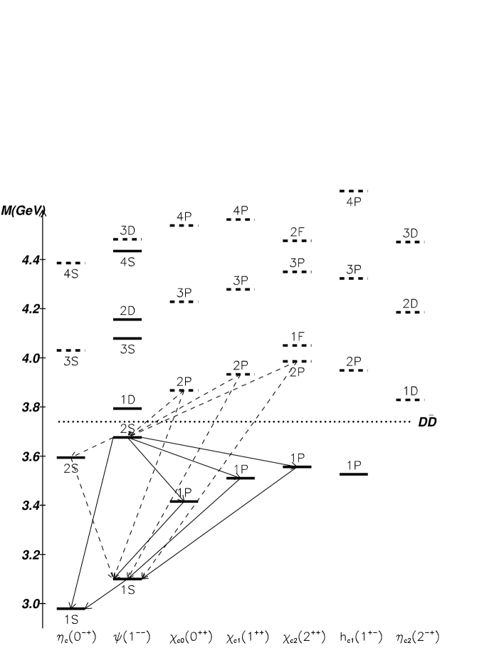
Figure 1: The $c\bar{c}$ levels in solution $I(c\bar{c})$. Solid lines stand for observed states, dashed lines for the predicted ones. Thin solid lines show the transitions included into fitting procedure, thin dashed line demonstrates the transitions, whose widths are predicted.

In Fig. 1, the levels for solution $I(c\bar{c})$ are shown for the mass region $M<4.5$ GeV. The wave functions for this solution are given in Appendix.

The obtained variants of solutions allow us to consider the status of $X(3872)$ and $Y(3941)$.

The solution $II(c\bar{c})$ provides for $\chi_{c1}(2P)$ the mass $3904$ MeV that is close to the value found in [9, 10, 11, 12] for the pick denoted as $X(3872)$. In agreement with $II(c\bar{c})$-solution, the analysis [26] favours the quantum numbers $J^{PC}=1^{++}$ for this state.

Still, one cannot exclude that $X(3872)$ is the $2^{-+}$-state (see [27] and references therein). In all solutions, the mass of $\eta_{c2}(1D)$ is lying in the interval $3815-3830$ MeV that demonstrates the plausibility of this variant as well.

The signal $Y(3941)$ does not contradict the hypothesis about its $2^{++}$ nature, because the mass of the $\chi_{2c}(2P)$ is close to $Y(3941)$ in all solutions.

2.2 Radiative transitions $(c\bar{c})_{in}\to\gamma+(c\bar{c})_{out}$

In Fig. 1, we show radiative decays which have been accounted for in the fitting procedure (corresonding formulae are presented in [1, 28]). For the levels below $D\bar{D}$ threshold, experimental data [25, 29, 30, 31] and the magnitudes of widths obtained in different versions of the fit are as follows (in keV):

Process Data $$I(c\bar{c})$$

1.10.3 2.877 4.853 1.4 4.216

16550 180.845 164.884 273.8 180.578

29590 291.536 297.362 391.8 289.569

390120 226.700 239.835 312.3 225.265

— 23.297 23.326 40.263 25.852

0.80.2 1.661 2.529 0.37 2.309

264 22.854 32.408 12.2 22.169

254 45.291 51.853 31.1 44.343

204 26.096 20.929 40.2 26.620

— 0.541 0.770 1.003 0.447

(10)

Note that the 20% accuracy is allowed for the transitions $\psi(2S)\to\gamma\chi_{cJ}(1P)$ and 30% one for $\chi_{cJ}(1P)\to\gamma\psi(1S)$ (we use a bit larger errors than those obtained in [31]). We also predict the widths of the decays $\eta_{c0}\to\gamma J/\psi$ and $\psi(2S)\to\gamma\eta_{c0}(2S)$.

The calculated values in (10) agree rather reasonably with the data.

The predictions of widths of the levels above the $D\bar{D}$ threshold (see Fig. 1) are as follows (widths are in keV):

Process Data $$I(c\bar{c})$$

— 9.181 5.841 0.468 12.612

— 48.130 50.831 28.797 59.013

— 56.911 72.080 31.331 67.713

— 81.851 73.158 92.450 73.925

— 212.937 221.604 290.379 192.502

— 154.796 176.599 197.162 144.714

(11)

2.3 The $c\bar{c}$ component of the photon wave function and two-photon radiative decays

In the fitting procedure, we approximate the vertex of the transition $\gamma\to c\bar{c}$ by the following formula:

$$G_{\gamma\to c\bar{c}(S)}(s)=\sum\limits_{n=1}^{6}C_{nS}G_{V(nS)}(s)+\frac{1}{1+\exp(-\beta_{\gamma}(s-s_{0}))}\ ,$$ (12)

$$G_{\gamma\to c\bar{c}(D)}(s)=\sum\limits_{n=1}^{2}C_{nD}G_{V(nD)}(s)\ ,$$

where $G_{V(nS)}(s)$ is the vertex for the transition $\psi(nS)\to c\bar{c}$ and $G_{V(nD)}(s)$ is the vertex for the transition $\psi(nD)\to c\bar{c}$, see [1] for the details. The parameters $C_{nS}$, $C_{nD}$, $\beta_{\gamma}$, $s_{0}$ for solutions $I(c\bar{c})$, $II(c\bar{c})$, $U(c\bar{c})$ and $R(c\bar{c})$ have been found as follows (in GeV):

$$I(c\bar{c})$$

= -10.100 = -9.073 = -3.852 = -14.990

= 2.121 = -0.252 = 0.476 = 3.416

= -0.373 = 0.038 = 0.325 = -0.862

= -1.818 = 0.217 = 0.667 = -1.834

= 9.998 = -1.158 = -2.571 = 11.704

= 3.369 = -0.529 = -0.707 = 0.305

= -0.031 = -0.005 = 0.080 = -0.186

= -0.110 = 0.020 = -0.082 = 0.114

= 2.85 = 2.85 = 2.85 = 2.85

= 18.79 = 18.79 = 18.79 = 18.79

(13)

The corresponding vertices $G_{\gamma\to c\bar{c}}(s)$ are shown in Fig. 2.

Figure 2: a) Vertices $G^{(S)}_{\gamma\to c\bar{c}}$ (a) and $G^{(D)}_{\gamma\to c\bar{c}}$ (b) for solutions $I(c\bar{c})$ (solid lines), $U(c\bar{c})$ (dashed lines) and $R(c\bar{c})$ (dotted lines).

Experimental values of partial widths [25, 32, 33, 34, 35] together with the widths obtained in the fitting procedure are shown below (in keV):

Process Data $$I(c\bar{c})$$

5.40 0.22 5.392 5.360 5.403 6.088

2.14 0.21 2.146 2.137 2.142 2.843

0.24 0.05 0.239 0.730 0.240 0.301

0.75 0.15 0.754 0.472 0.749 1.210

0.47 0.10 0.472 0.236 0.469 0.113

0.77 0.23 0.771 0.763 0.770 0.915

(14)

With the determined vertices for $G_{\gamma\to c\bar{c}}(s)$, we can obtain the widths of the two-photon decays (see [1] for more detail). The comparison of experimentally measured widths with those obtain in our calculations is given below:

Process Data $$I(c\bar{c})$$

7.00.9 6.971 6.808 7.002 7.088

2.60.5 2.426 2.620 2.578 2.212

1.020.400.17(L3 ) 0.558 0.528 0.068 5.706

1.760.470.40(OPAL)

1.080.300.26(CLEO)

0.330.080.06(E760)

(15)

Let us emphasize that the data do not tell us definitely about the width $\chi_{c2}(3556)\to\gamma\gamma$. In the reaction $p\bar{p}\to\gamma\gamma$, the value $\Gamma(\chi_{2}(3556)\to\gamma\gamma)=0.32\pm 0.080\pm 0.055$ keV was obtained in [35], while in direct measurements such as $e^{+}e^{-}$ annihilation the width is much larger: $1.02\pm 0.40\pm 0.17\;{\rm keV}$ [32] , $1.76\pm 0.47\pm 0.40\;{\rm keV}$ [33]  , $1.08\pm 0.30\pm 0.26\;{\rm keV}$ [34]  . The compilation [25] provides us with the value close to that of [35]. The value found in our fit agrees with data reported by [32, 33, 34] and contradicts the magnitude from [35].

Our predictions of widths $c\bar{c}\to\gamma\gamma$ for the levels below $4$ GeV are as follows:

Process Data $$I(c\bar{c})$$

— 12.234 11.947 12.289 12.439

— 2.142 2.313 2.276 1.953

— 0.500 0.473 0.061 5.111

(16)

In tables 1,2,3, we compare our results with those obtained by other authors.

In [36], the calculated widths depend on a chosen gauge for the gluon exchange interaction — we demonstrate the results obtained for both Feynman (F) and Coulomb (C) gauges.

In [37], the $c\bar{c}$ system was studied in terms of scalar (S) and vector (V) confinement forces — both variants are presented in tables 1,2,3. The results obtained in the nonrelativistic approach to the $c\bar{c}$ system [38] are also shown in tables 1,2,3.

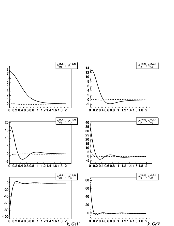
Figure 3: Wave functions for $\psi(nS)$ in solution $I(c\bar{c})$. Solid lines stand for $\psi^{(1,0,1)}_{n}$ and dashed ones for $\psi^{(1,2,1)}_{n}$. All magnitudes are in GeV units.

In both relativistic [36, 37] and nonrelativistic [38] approaches, there is rather large discrepancy between the data and calculated values of $\psi(nS)\to e^{+}e^{-}$ (in [36] the width of the transition $J/\psi\to e^{+}e^{-}$ was fixed with the use of a subtraction parameter). In our opinion, the reason is that in all above-mentioned papers, soft interaction of quarks was not accounted for — we mean the processes shown in Fig. 3b,c of Ref. [1]. In fact, the necessity of taking into consideration the low-energy quark interaction was understood decades ago but untill now this procedure has not become commonly accepted even for light quarks; see, for example, [39, 40].

Table 1: Comparison of data for the transitions $(c\bar{c})_{in}\to\gamma+(c\bar{c})_{out}$ with our results and calculations of other groups (the width is given in keV).

Decay	Data	$I(c\bar{c})$	LS(F)[36]	LS(C)[36]	RM(S)[37]	RM(V)[37]	NR[38]
$J/\psi(1S)\to\eta_{c0}(1S)\gamma$	1.1$\pm$0.3	3.4	1.7–1.3	1.7–1.4	3.35	2.66	1.21
$\psi(2S)\to\chi_{c0}(1P)\gamma$	26$\pm$4	23	31–47	26–31	31	32	19.4
$\psi(2S)\to\chi_{c1}(1P)\gamma$	25$\pm$4	45	58–49	63–50	36	48	34.8
$\psi(2S)\to\chi_{c2}(1P)\gamma$	20$\pm$4	26	48–47	51–49	60	35	29.3
$\psi(2S)\to\eta_{c0}(1S)\gamma$	0.8$\pm$0.2	2.0	11–10	10–13	6	1.3	4.47
$\chi_{c0}(1P)\to J/\psi(1S)\gamma$	165$\pm$50	181	130–96	143–110	140	119	147
$\chi_{c1}(1P)\to J/\psi(1S)\gamma$	295$\pm$90	292	390–399	426–434	250	230	287
$\chi_{c2}(1P)\to J/\psi(1S)\gamma$	390$\pm$120	227	218–195	240–218	270	347	393

Table 2: Decay widths $\psi\to e^{+}e^{-}$, our results and those of other groups v.s. data (in keV).

Decay	Data	$I(c\bar{c})$	LS(F)[36]	LS(C)[36]	RM(S)[37]	RM(V)[37]	NR[38]
$J/\psi(1S)\to e^{+}e^{-}$	5.40 $\pm$ 0.22	5.39	5.26	5.26	8.05	9.21	12.2
$\psi(2S)\to e^{+}e^{-}$	2.14 $\pm$ 0.21	2.15	2.8–2.5	2.9–2.7	4.30	5.87	4.63
$\psi(1D)\to e^{+}e^{-}$	0.24 $\pm$ 0.05	0.24	2.0–1.6	2.1–1.8	3.05	4.81	3.20
$\psi(3S)\to e^{+}e^{-}$	0.75 $\pm$ 0.15	0.75	1.4–1.0	1.6–1.3	2.16	3.95	2.41
$\psi(2D)\to e^{+}e^{-}$	0.47 $\pm$ 0.10	0.47	—	—	—	—	—
$\psi(4S)\to e^{+}e^{-}$	0.77 $\pm$ 0.23	0.77	—	—	—	—	—

Table 3: Decay widhs $(c\bar{c})_{in}\to\gamma+(c\bar{c})_{out}$ in the region below $4$ GeV (in keV)

Decay	Data	$I(c\bar{c})$	LS [36]	[41]	[42]	[43]	[44]	[45]	[46]
$\eta_{c}(1S)\to\gamma\gamma$	7.0$\pm$0.9	6.9	6.2–6.3 (F,C)	5.5	3.5	10.9	7.8	5.5	4.8
$\eta_{c}(1S)\to\gamma\gamma$	—	12.2	–	1.8	1.38	–	3.5	2.1	3.7
$\chi_{c0}(1P)\to\gamma\gamma$	2.6$\pm$0.5	2.4	1.5–1.8 (F,C)	2.9	1.39	6.4	2.5	5.32	–
$\chi_{c0}(1P)\to\gamma\gamma$	—	2.1	—	1.9	1.11	–	–	–	–
$\chi_{c2}(1P)\to\gamma\gamma$	1.02$\pm$0.40$\pm$0.17[32]	0.61	0.3–0.4 (F,C)	0.50	0.44	0.57	0.28	0.44	–
	1.76$\pm$0.47$\pm$0.40[33]
	1.08$\pm$0.30$\pm$0.26[34]
	0.33$\pm$0.08$\pm$0.06[35]
$\chi_{c2}(1P)\to\gamma\gamma$	—	0.5	—	0.52	0.48	–	–	–	–

3 Conclusion

We have performed a successful description of both $c\bar{c}$ levels and their radial excitation transitions for several interaction variants as follows: for scalar confinement potential, scalar and vector confinement potential in case of instantaneous and retardation forces. Such a diversity in the choice of forces reflects the lack of available experimental data to guarantee unambiguous determination of the interaction. First of all, one misses the data for the radiative $c\bar{c}$ decays. This is why we pay special attention to the predictions given by different versions of our calculations.

Rather good description of the $c\bar{c}$ levels being obtained, the wave functions related to different solutions may noticeably differ from each other, and sometimes they demonstrate rather unusual behaviour. Because of that, we pay a considerable attention to the presentation of wave functions of the $c\bar{c}$ systems. We think that the future progress in understanding the $c$-quark interactions in the soft region is related precisely to a better knowledge of wave functions, that should be based on further study of radiative transitions.

4 Appendix. Wave function of the $c\bar{c}$ sector

**

Tables 4–10 give us the $c_{i}(S,L,J;n)$ coefficients, which determine the wave functions $\psi^{(S,L,J)}$ for solution $I(c\bar{c})$ according to the following formula:

$$\psi^{(S,L,J)}_{(n)}(k^{2})=e^{-\beta k^{2}}\sum\limits_{i=1}^{9}c_{i}(S,L,J;n)k^{i-1}\,,$$

where $k^{2}\equiv{\bf k}^{2}$ (recall that $s=4m^{2}+4{\bf k}^{2}$). The fitting parameter $\beta$ is of the order of $0.5-1.5$ GeV^-2 and it may be different in different flavor sectors; we put $\beta=1.2$ GeV^-2. In tables, we also show $W_{LL^{\prime}}$’s, which enter the normalization condition $W_{LL}+W_{LL^{\prime}}+W_{L^{\prime}L^{\prime}}=1$, being the convolution of the wave functions

$$W_{L,L^{\prime}}=\psi^{(S,L,J)}\otimes\psi^{(S,L^{\prime},J)}\ ,$$

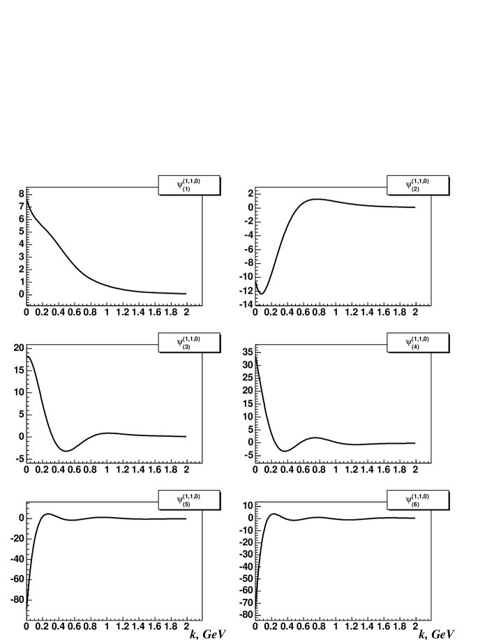
Figure 5: Wave functions for $\eta_{c}$ in solution $I(c\bar{c})$.

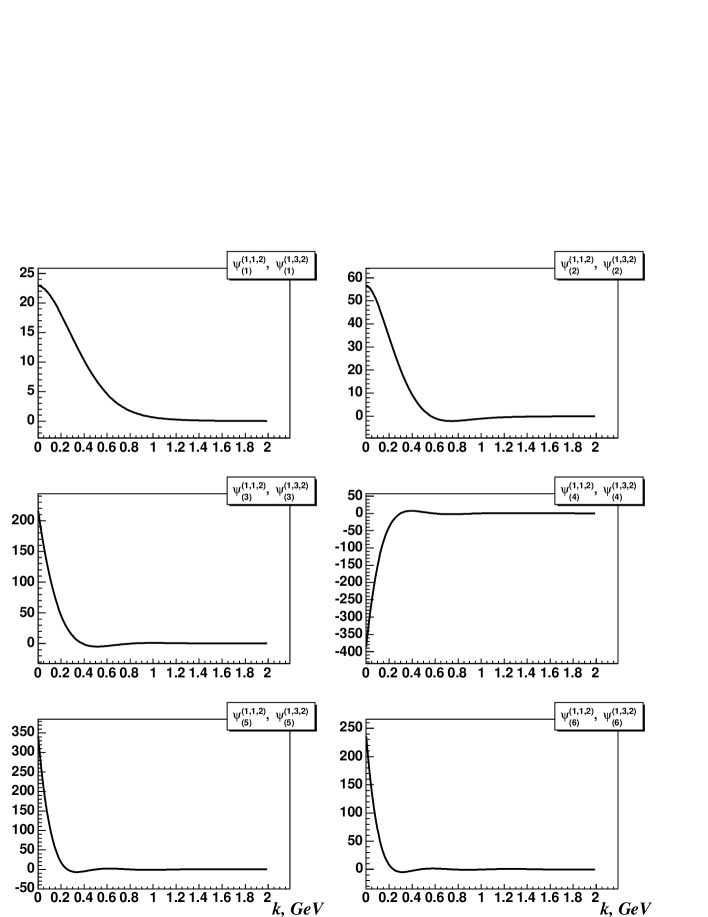
Figure 7: Wave functions for $\chi_{c1}$ in solution $I(c\bar{c})$.

see [1] for more detail. In Figs. 3–9, we demonstrate these wave functions.

Table 4: Constants $c_{i}(S,L,J;n)$ from Eq. (4) (in GeV units) for the wave functions of $\Upsilon$-mesons in solution $I(c\bar{c})$

	$\Psi(1S)$		$\Psi(2S)$		$\Psi(3S)$
	$W_{00}\qquad W_{02}\qquad W_{22}$		$W_{00}\qquad W_{02}\qquad W_{22}$		$W_{00}\qquad W_{02}\qquad W_{22}$
	0.99987   -0.00066   0.00079		0.99924   -0.00174   0.00250		0.99807   -0.00288   0.00481
$i$	$\psi^{(1,0,1)}$	$\psi^{(1,2,1)}$	$\psi^{(1,0,1)}$	$\psi^{(1,2,1)}$	$\psi^{(1,0,1)}$	$\psi^{(1,2,1)}$
1	7.9009	-5.9190	11.6473	1.5241	17.3698	-30.6053
2	-6.0655	34.4862	47.6240	-14.8598	41.6854	199.5601
3	16.7028	-83.5239	-453.2935	41.5693	-860.2544	-499.8739
4	-105.4498	102.1413	1094.1453	-41.5148	2693.3655	625.7537
5	224.9337	-63.9523	-1334.8514	2.7143	-3793.6194	-415.9994
6	-231.2288	16.2702	943.6424	24.1754	2870.7394	134.3492
7	127.1267	1.9716	-393.8494	-18.1178	-1206.4102	-9.1646
8	-36.0487	-1.8633	90.4811	5.3507	264.5053	-5.3519
9	4.1617	0.2684	-8.8655	-0.5785	-23.4715	0.9886
	$\Psi(4S)$		$\Psi(5S)$		$\Psi(6S)$
	$W_{00}\qquad W_{02}\qquad W_{22}$		$W_{00}\qquad W_{02}\qquad W_{22}$		$W_{00}\qquad W_{02}\qquad W_{22}$
	0.99166   -0.00737   0.01570		0.99889   -0.00450   0.00561		0.95583   -0.02419   0.06835
$i$	$\psi^{(1,0,1)}$	$\psi^{(1,2,1)}$	$\psi^{(1,0,1)}$	$\psi^{(1,2,1)}$	$\psi^{(1,0,1)}$	$\psi^{(1,2,1)}$
1	36.5862	-1.1743	-95.0826	-9.0172	78.7073	62.0712
2	-212.7589	51.7345	1136.7086	81.4929	-1113.5476	-481.4354
3	-6.8022	-243.2839	-4872.0833	-284.5462	5651.5790	1419.5113
4	1855.8350	448.2876	10215.8015	523.5176	-13997.7499	-2062.1487
5	-4206.0402	-401.5179	-11814.1052	-570.3848	18993.0373	1573.0804
6	4182.8669	178.7153	7907.6179	381.1356	-14736.1180	-594.8321
7	-2151.4758	-31.8182	-3052.3529	-152.6765	6486.3763	71.5608
8	559.1998	-1.4693	631.1276	33.4538	-1501.0222	15.2345
9	-58.1665	0.8430	-54.2492	-3.0632	141.2673	-3.6824
	$\Psi(1D)$		$\Psi(2D)$		$\Psi(3D)$
	$W_{00}\qquad W_{02}\qquad W_{22}$		$W_{00}\qquad W_{02}\qquad W_{22}$		$W_{00}\qquad W_{02}\qquad W_{22}$
	0.00435   -0.00169   0.99734		0.00736   -0.00316   0.99581		0.00697   -0.00433   0.99736
$i$	$\psi^{(1,2,1)}$	$\psi^{(1,0,1)}$	$\psi^{(1,2,1)}$	$\psi^{(1,0,1)}$	$\psi^{(1,2,1)}$	$\psi^{(1,0,1)}$
1	84.4242	-0.1030	313.1175	-0.2904	467.5023	-1.8858
2	-205.1653	3.1892	-1319.9899	10.2284	-2389.2054	23.4791
3	181.7717	-19.8052	2113.8219	-70.5461	4394.0661	-121.9462
4	-77.1585	46.4276	-1592.4362	192.4214	-3418.8591	332.6430
5	49.8493	-58.9700	460.0515	-260.8978	524.5556	-507.1882
6	-57.6810	44.8041	111.8270	194.4329	907.2750	442.0815
7	35.7092	-20.4094	-120.5831	-80.7753	-629.5731	-218.2705
8	-10.1511	5.1363	32.7133	17.4329	163.7261	56.6805
9	1.0906	-0.5496	-3.1245	-1.5051	-15.6276	-6.0100
	$\Psi(4D)$		$\Psi(5D)$		$\Psi(6D)$
	$W_{00}\qquad W_{02}\qquad W_{22}$		$W_{00}\qquad W_{02}\qquad W_{22}$		$W_{00}\qquad W_{02}\qquad W_{22}$
	0.02465   -0.01134   0.98669		0.01698   -0.01676   0.99978		0.02212   -0.01885   0.99673
$i$	$\psi^{(1,2,1)}$	$\psi^{(1,0,1)}$	$\psi^{(1,2,1)}$	$\psi^{(1,0,1)}$	$\psi^{(1,2,1)}$	$\psi^{(1,0,1)}$
1	413.1586	8.8245	-289.4977	1.5578	244.8123	3.7011
2	-2384.9885	-114.1754	1734.9402	-22.5966	-1545.0640	-63.3077
3	4895.6915	524.1161	-3619.8761	127.1963	3437.6769	378.8322
4	-4120.8799	-1159.3614	2815.1704	-371.5994	-2942.2393	-1087.4587
5	490.3119	1390.2561	415.7821	619.5920	-231.3078	1690.6255
6	1523.0854	-947.6269	-2036.6024	-602.2710	2146.9545	-1488.8664
7	-1076.5260	366.2696	1288.9620	332.9247	-1496.2120	736.8267
8	293.9187	-74.6692	-343.3866	-96.0393	431.2140	-189.8749
9	-29.5824	6.2449	34.1359	11.1873	-46.2070	19.7831

Table 5: Constants $c_{i}(S,L,J;n)$ from Eq. (4) (in GeV) for the wave functions of $\chi_{c2}$-mesons in solution $I(c\bar{c})$

	$\chi_{c2}(1P)$		$\chi_{c2}(2P)$		$\chi_{c2}(3P)$
	$W_{11}\qquad W_{13}\qquad W_{33}$		$W_{11}\qquad W_{13}\qquad W_{33}$		$W_{11}\qquad W_{13}\qquad W_{33}$
	0.99952   -0.00070   0.00118		0.99765   -0.00211   0.00446		0.99209   -0.00518   0.01309
$i$	$\psi^{(1,1,2)}$	$\psi^{(1,3,2)}$	$\psi^{(1,1,2)}$	$\psi^{(1,3,2)}$	$\psi^{(1,1,2)}$	$\psi^{(1,3,2)}$
1	-17.5035	9.0856	4.5957	39.0522	-93.1247	44.4200
2	-86.9407	-40.9452	-623.9524	-250.9432	163.8698	-311.5971
3	506.5360	85.1047	3316.2121	629.3054	1317.7565	796.6134
4	-988.9820	-100.6670	-7222.9252	-821.2865	-5066.0027	-990.8076
5	1026.3189	71.0253	8391.4505	608.6930	7472.6180	644.8615
6	-625.3392	-29.4658	-5639.3954	-257.5492	-5744.7189	-202.3282
7	224.1992	6.6484	2197.9985	57.7459	2434.8192	13.3976
8	-43.7175	-0.6473	-460.8963	-5.2652	-539.0269	7.5182
9	3.5664	0.0062	40.1760	-0.0143	48.6569	-1.3447
	$\chi_{c2}(4P)$		$\chi_{c2}(5P)$		$\chi_{c2}(6P)$
	$W_{11}\qquad W_{13}\qquad W_{33}$		$W_{11}\qquad W_{13}\qquad W_{33}$		$W_{11}\qquad W_{13}\qquad W_{33}$
	0.88640   -0.00477   0.11837		0.98493   -0.01273   0.02780		0.93818   -0.03946   0.10128
$i$	$\psi^{(1,1,2)}$	$\psi^{(1,3,2)}$	$\psi^{(1,1,2)}$	$\psi^{(1,3,2)}$	$\psi^{(1,1,2)}$	$\psi^{(1,3,2)}$
1	638.6609	391.6378	-134.7570	-221.6602	117.7874	104.0293
2	-5864.8034	-2008.6939	1751.9157	1250.1138	-1488.3254	-706.9778
3	21108.8607	4224.3629	-8121.0456	-2766.6069	6956.8543	1877.3877
4	-39600.9145	-4709.0719	18375.8266	3074.1617	-16174.3244	-2509.6472
5	42944.0995	2957.4768	-22896.3579	-1771.0161	20877.3955	1793.4813
6	-27861.8978	-999.8571	16466.2322	434.8957	-15563.0676	-647.3392
7	10649.1787	137.5405	-6796.9738	31.0544	6631.3660	78.8171
8	-2206.5653	8.3919	1492.7938	-36.5787	-1494.2661	13.2404
9	190.7603	-3.1287	-134.9738	5.1157	137.6804	-3.2854
	$\chi_{c2}(1F)$		$\chi_{c2}(2F)$		$\chi_{c2}(3F)$
	$W_{11}\qquad W_{13}\qquad W_{33}$		$W_{11}\qquad W_{13}\qquad W_{33}$		$W_{11}\qquad W_{13}\qquad W_{33}$
	0.00301   -0.00135   0.99834		0.10992   -0.00454   0.89462		0.03903   -0.01166   0.97263
$i$	$\psi^{(1,3,2)}$	$\psi^{(1,1,2)}$	$\psi^{(1,3,2)}$	$\psi^{(1,1,2)}$	$\psi^{(1,3,2)}$	$\psi^{(1,1,2)}$
1	-242.7471	10.5652	-565.8475	225.5515	733.1238	19.8324
2	744.2459	-95.8214	2117.9502	-2067.2776	-3370.3257	-120.2819
3	-845.6564	355.4159	-2625.9078	7468.3409	5512.4695	179.6152
4	320.2998	-686.5646	638.7903	-14099.5057	-3448.4647	157.0118
5	166.8886	763.7615	1409.3867	15396.8275	-410.2084	-688.2629
6	-224.3091	-506.8350	-1486.9023	-10057.8914	1736.5500	755.6477
7	96.3257	197.7245	638.6645	3868.9470	-956.7876	-394.8955
8	-19.3136	-41.7533	-131.7223	-806.4039	226.5196	101.4201
9	1.5203	3.6750	10.7017	70.0913	-20.3853	-10.2876
	$\chi_{c2}(4F)$		$\chi_{c2}(5F)$		$\chi_{c2}(6F)$
	$W_{11}\qquad W_{13}\qquad W_{33}$		$W_{11}\qquad W_{13}\qquad W_{33}$		$W_{11}\qquad W_{13}\qquad W_{33}$
	0.01125   -0.00896   0.99771		0.01670   -0.01856   1.00186		0.01548   -0.02033   1.00485
$i$	$\psi^{(1,3,2)}$	$\psi^{(1,1,2)}$	$\psi^{(1,3,2)}$	$\psi^{(1,1,2)}$	$\psi^{(1,3,2)}$	$\psi^{(1,1,2)}$
1	-580.3877	-12.4060	431.6178	1.5693	345.9078	5.2688
2	2948.0418	137.4061	-2289.0231	-16.1472	-1924.9704	-74.4252
3	-5368.6253	-566.3875	4363.4753	50.9676	3911.9978	376.9102
4	3893.8813	1161.4946	-3306.3734	-47.7121	-3311.2035	-935.6268
5	3.8221	-1320.6326	-27.4883	-46.6674	358.9932	1279.4826
6	-1709.0721	866.8103	1606.1715	127.5496	1343.8856	-1004.6984
7	1047.0953	-325.6228	-1012.8337	-98.5000	-964.7262	448.1251
8	-263.5517	64.7935	261.2351	33.0133	268.3202	-104.9359
9	24.8409	-5.2798	-25.0732	-4.1196	-27.3899	9.9921

Table 6: Constants $c_{i}(S,L,J;n)$ from eq. (4) (in GeV) for the wave functions of $\eta_{c0}$, $\chi_{c0}$, $\chi_{c1}$ and $h_{c1}$ mesons in solution $I(c\bar{c})$

$i$	$\eta_{c0}(1P)$	$\eta_{c0}(2P)$	$\eta_{c0}(3P)$	$\eta_{c0}(4P)$	$\eta_{c0}(5P)$	$\eta_{c0}(6P)$
1	7.6494	-10.5636	18.1089	33.6294	-89.2312	-75.5014
2	-23.0211	-53.9217	15.0118	-170.0167	1032.3991	1029.1523
3	124.2754	461.0285	-623.7988	-168.7223	-4276.2522	-5025.8538
4	-395.6413	-1133.8010	1908.5781	2060.7362	8662.4563	11959.9547
5	656.5275	1456.7298	-2536.9289	-4211.5707	-9688.9143	-15569.2648
6	-605.5583	-1101.1359	1780.5781	3997.5023	6289.9521	11572.6965
7	314.7296	493.4357	-680.8186	-1997.5324	-2365.3552	-4872.6646
8	-86.2318	-121.2544	132.0261	509.0043	479.4585	1076.4010
9	9.7057	12.6004	-9.8555	-52.2319	-40.7532	-96.3877
$i$	$\chi_{c0}(1P)$	$\chi_{c0}(2P)$	$\chi_{c0}(3P)$	$\chi_{c0}(4P)$	$\chi_{c0}(5P)$	$\chi_{c0}(6P)$
1	-17.8495	-50.2837	-151.3174	-313.0348	318.7744	-249.2578
2	3.8696	5.7940	731.5190	2334.3640	-2879.7647	2448.4531
3	29.1978	634.0603	-1074.8942	-6487.9099	9875.5585	-9126.1510
4	70.7786	-1637.8698	270.8311	8844.2446	-17101.9307	17108.1285
5	-273.1091	1949.8183	727.7711	-6388.0162	16610.2166	-17802.3919
6	321.4758	-1315.0808	-767.5997	2335.4592	-9396.2245	10577.7296
7	-184.1650	521.0477	313.2245	-289.9459	3061.3295	-3502.4000
8	52.5331	-113.9435	-55.4903	-50.4060	-530.9090	584.2914
9	-5.9970	10.6960	3.0610	13.0531	37.9718	-36.1088
$i$	$\chi_{c1}(1P)$	$\chi_{c1}(2P)$	$\chi_{c1}(3P)$	$\chi_{c1}(4P)$	$\chi_{c1}(5P)$	$\chi_{c1}(6P)$
1	23.0070	56.7513	217.3310	-388.4208	344.6565	238.1913
2	-3.8670	-14.0364	-1332.2767	3249.2463	-3365.3754	-2490.3066
3	-115.4587	-778.7437	3058.3410	-10453.2199	12574.5044	9950.4054
4	191.1470	2115.0575	-3497.5882	17295.2284	-23976.3393	-20229.2674
5	-112.1101	-2567.5452	2172.1531	-16412.7705	25956.4509	23216.4628
6	4.4321	1719.1521	-716.3965	9284.6416	-16581.9431	-15583.6367
7	23.5865	-657.5312	101.6710	-3089.5089	6182.0939	6036.8548
8	-9.8945	134.9058	1.4698	556.8344	-1242.3831	-1245.5237
9	1.2824	-11.5449	-1.2720	-41.8049	103.9046	105.5852
$i$	$h_{c}(1P)$	$h_{c}(2P)$	$h_{c}(3P)$	$h_{c}(4P)$	$h_{c}(5P)$	$h_{c}(6P)$
1	-19.4824	44.2886	130.8468	-296.9419	431.5082	-293.9990
2	-42.1580	119.7469	-553.3042	2284.4817	-4002.0767	2983.8574
3	305.3320	-1319.3114	298.1904	-6661.4528	14363.1096	-11699.4557
4	-573.6405	3202.4192	1602.7564	9794.3567	-26533.5962	23525.9355
5	548.0217	-3792.3619	-3269.2777	-8048.5695	28014.7411	-26866.9716
6	-299.4493	2527.4497	2752.3010	3805.6849	-17540.3649	18029.3913
7	93.8170	-967.1883	-1199.8706	-1003.0218	6432.1760	-7008.3077
8	-15.4547	198.4952	266.1679	130.1848	-1274.7649	1455.2756
9	1.0081	-16.9394	-23.7422	-5.6569	105.3324	-124.4976

Figure 4: Wave functions for $\psi(nD)$ in solution $I(c\bar{c})$. Solid lines stand for $\psi^{(1,2,1)}_{n}$ and dashed ones for $\psi^{(1,0,1)}_{n}$. All magnitudes are in GeV units.

Figure 6: Wave functions for $\chi_{c0}$ in solution $I(c\bar{c})$.

Figure 8: Wave functions for $\chi_{c2}$ in solution $I(c\bar{c})$. Solid lines stand for $\psi^{(1,1,2)}_{n}$ and dashed ones for $\psi^{(1,3,2)}_{n}$.

Figure 9: Wave functions for $\chi_{c2}$ in Solution $I(c\bar{c})$. Solid lines stand for $\psi^{(1,3,2)}_{n}$ and dashed ones for $\psi^{(1,1,2)}_{n}$.

References

- [1] V.V. Anisovich, L.G. Dakhno, M.A. Matveev, V.A. Nikonov, and A.V. Sarantsev, hep-ph/0510410.
- [2] A.V. Anisovich, V.V. Anisovich, B.N. Markov, M.A. Matveev, and A.V. Sarantsev, Yad. Fiz. 67, 794 (2004) [Phys. of Atomic Nuclei, 67, 773 (2004)].
-
[3]
V.V. Anisovich, M.N. Kobrinsky, D.I. Melikhov, and
A.V. Sarantsev, Nucl. Phys. A 544, 747 (1992);
A.V. Anisovich and V.A. Sadovnikova, Yad. Fiz. 55, 2657 (1992); 57, 75 (1994); Eur. Phys. J. A 2, 199 (1998). - [4] V.V. Anisovich, D.I. Melikhov, and V.A. Nikonov, Phys. Rev. D 52, 5295 (1995); D 55, 2918 (1997).
- [5] A.V. Anisovich, V.V. Anisovich, and V.A. Nikonov, Eur. Phys. J. A 12, 103 (2001).
- [6] A.V. Anisovich, V.V. Anisovich, V.N. Markov, and V.A. Nikonov, Yad. Fiz. 65, 523 (2002) [Phys. Atom. Nucl. 65, 497 (2002)].
- [7] A.V. Anisovich, V.V. Anisovich, M.A. Matveev, and V.A. Nikonov, Yad. Fiz. 66, 946 (2003) [Phys. Atom. Nucl. 66, 914 (2003)].
- [8] V.V. Anisovich, L.G. Dakhno, M.N. Markov, V.A. Nikonov, and A.V. Sarantsev, Yad. Fiz., in press; hep-ph/0406320, hep-ph/0410361.
- [9] S.K. Choi at. al., (Belle Collab.), Phys. Rev. Lett. 91, 262001 (2003).
- [10] D. Acosta at. al., (CDF II Collab.), Phys. Rev. Lett. 93, 072001 (2004).
- [11] V.M.Abrazov at. al., (D0 Collab.), Phys. Rev. Lett. 93, 162002 (2004).
- [12] B. Aubert at. al., (Barbar Collab.), Phys. Rev. D 71, 071103 (2005).
- [13] N.A. Törnqvist, arXiv:hep-ph/0402237.
- [14] F.E. Close and P.R. Page, Phys. Lett. B 578, 119 (2004).
- [15] M.B. Voloshin, Phys. Lett. B 579, 316 (2004).
- [16] C.Z. Yuan, X.M. Mo and P. Wang, Phys. Lett. B 579, 74 (2004).
- [17] C.-Y. Wong, Phys. Rev. C 69, 055202 (2004).
- [18] T. Barnes and S. Godfrey, Phys. Rev. D 69, 054008 (2004).
- [19] E.S. Swanson, Phys. Lett. B 588, 189 (2004).
- [20] T. Skwarnicki, arXiv:hep-ph/0311243.
- [21] P. Bicudo, arXiv:hep-ph/0401106.
- [22] E.J. Eichten, K. Lane and C. Quigg, Phys. Rev. D 69, 094019 (2004).
- [23] N. Isgur and M.B. Wiss, Phys. Lett. B 232, 113 (1989); Phys. Lett. B 237, 527 (1990).
- [24] A.V. Monohar and C.T. Sachrajda, Phys. Lett. B 592, 473 (2004).
- [25] S. Eidelman, et al., Phys. Lett. B 592, 1 (2004).
- [26] D.V. Bugg, Phys. Rev. D 71, 016006, (2005).
- [27] T. Barnes and S. Godfrey, Phys. Rev. D 69, 054008, (2004).
- [28] A.V. Anisovich, V.V. Anisovich, M.A. Matveev, V.N. Markov, V.A. Nikonov, and A.V. Sarantsev, J. Phys. G: Nucl. Part. Phys., in press; hep-ph/0509042.
- [29] J. Gaiser, et al., Phys. Rev. D 34, 711 (1986).
- [30] C.J. Biddick, et al., Phys. Rev. Lett. 38, 1324 (1977).
- [31] J.J. Hernández-Rey, S. Navas, and C. Patrignani, Phys. Lett. B 952, 822 (2004).
- [32] M. Acciari, et al., Phys. Lett. B 453, 73 (1999).
- [33] K. Ackerstaff, et al., Phys. Lett. B 439, 197 (1998).
- [34] J. Dominick, et al., Phys. Rev. D 50, 4265 (1994).
- [35] T.A. Armstrong, et al., Phys. Rev. Lett. 70, 2988 (1993).
- [36] J. Linde and H. Snellman, Nucl. Phys. A 619, 346 (1997).
- [37] J. Resag and C.R. Münz, Nucl. Phys. A 590, 735 (1995).
- [38] M.Beyer, U. Bohn, M.G. Huber, B.C. Metsch, and J. Resag, Z.Phys C 55, 307 (1992).
- [39] M.A. DeWitt, H.M. Choi and C.R. Ji, Phys. Rev. D68: 054026 (2003).
- [40] B.-W. Xiao and B.-Q. Ma, Phys. Rev. D 68, 034020 (2003).
- [41] D. Ebert, R.N. Faustov, and V.O. Galkin, Phys. Rev D 67, 014027 (2003).
- [42] S.N. Münz, Nucl. Rhys. A 609, 364 (1996).
- [43] S.N. Gupta, S.F. Radford, and W.W. Repko, Phys. Rev. D 54, 2075 (1996).
- [44] G.A. Schuler, F.A Berends, and R. van Gulik, Nucl. Rhys. B 523, 423 (1998).
- [45] H.-W. Huang, et. al. Phys. Rev. D 54, 2123 (1996); D 56, 368 (1997).
- [46] E.S. Ackleh, T. Barnes, et al., Phys. Rev. D 45, 232 (1992).