Abstract

We reconsider the idea of identifying the Higgs field as the internal component of a gauge field in the flat space $R^{4}\times S^{1}/{\bf Z}_{2}$, by relaxing the constraint of having unbroken SO(4,1) Lorentz symmetry in the bulk. In this way, we show that the main common problems of previous models of this sort, namely the prediction of a too light Higgs and top mass, as well as of a too low compactification scale, are all solved. We mainly focus our attention on a previously constructed model. We show how, with few minor modifications and by relaxing the requirement of SO(4,1) symmetry, a potentially realistic model can be obtained with a moderate tuning in the parameter space of the theory. In this model, the Higgs potential is stabilized and the hierarchy of fermion masses explained.

1 Introduction

The Electroweak Symmetry Breaking (EWSB) mechanism and the hierarchy of fermion masses are among the most obscure aspects of the Standard Model (SM). The minimal set-up of a single doublet scalar field (the SM Higgs field) which drives the EWSB is affected by a stability problem at the quantum level, since the Higgs mass term is quadratically sensitive to the scale of new physics. In the SM, moreover, the observed fermion masses are obtained by an unnatural choice of Yukawa couplings. Even leaving aside the three neutrinos, their values range from $\sim 10^{-5}-10^{-6}$ for the electron up to $\sim 1$ for the top quark.

Looking for alternative theories in which these problems are solved has been one of the main guidelines for new ideas and models beyond the SM. Supersymmetry (SUSY) is certainly the most interesting and well motivated possibility. It predicts the unification of gauge couplings, it naturally incorporates a good candidate to explain the dark matter abundance in the universe and, if assumed to be broken at energy scales $\sim$ few TeV, it can also give rise to a natural EWSB. Last, but not least, it is a weakly coupled theory. The simplest model of this sort is the Minimal Supersymmetric Standard Model (MSSM). Despite the above important positive aspects, superparticles have not been discovered yet and, in fact, most of the parameter space of the MSSM is already experimentally ruled out, resulting in an unwanted fine-tuning in the model. Moreover, the MSSM does not provide a sensible explanation for the hierarchy of SM fermion masses. This motivates the quest for other ideas and models, also alternative to SUSY, which can explain the stability of the EWSB scale and the hierarchy of fermion masses.

Models where the Higgs field is identified with the internal component of a gauge field in TeV–sized extra dimensions [2] (also known as models with gauge-Higgs unification) are an example of this sort [3, 4] (see [5] for earlier references and [6] for a brief overview). The higher dimensional gauge symmetry, rather than SUSY, provides the stabilization of the Higgs mass term. Consequently, the quadratic divergencies in the Higgs mass due to the SM particles are cancelled by states with the same statistic, and not opposite as in SUSY. This is analogous to what typically happens in little Higgs models [7], which indeed arose from the deconstructed version of gauge-Higgs unification models [8]. The five-dimensional (5D) case, with one extra dimension, is the simplest one and also the one which seems phenomenologically more appealing. It is by now clear how to embed the SM fermions and to break the flavour symmetry in such framework, despite the fact that the Yukawa couplings are gauge couplings: one can either put the SM fermions on the boundaries and couple them to massive bulk fermions [9, 10] or one can identify the SM fields as the (chiral) zero modes of bulk fermions with jumping mass terms [11, 4]. In both cases one ends up with a concrete realization of the idea of getting small Yukawa couplings by means of exponentially small overlaps of wave functions in the internal space [12]. Models defined in flat space seem to have common drawbacks. Namely, one obtains too low Higgs, top and compactification masses. To solve these problems, one has to find a gauge-invariant way to increase the (gauge) couplings of the Higgs with the bulk fermions. Two known possibilities are the introduction of large localized gauge kinetic terms [9] and warped compactification [13]. In both cases, however, the bulk wave functions are distorted in a non-trivial way, resulting in potentially too large deviations from the SM coming from the Electroweak Precision Tests (EWPT) and the universality of gauge couplings. Implementing a custodial symmetry improves the situation, but some fine tuning is still necessary to get viable models. An interesting proposal along this direction has been provided in [14].

In this paper we propose a different approach to get a potentially realistic model with gauge-Higgs unification in flat space. The essential ingredient which we advocate is an explicit tree–level breaking of the Lorentz SO(4,1) symmetry. More precisely, we notice that another possible way to increase the couplings between the Higgs field and the fermions in a 5D gauge-invariant way is achieved by breaking the SO(4,1)/SO(3,1) symmetry (so that the usual SO(3,1) Lorentz symmetry is unbroken), which is the one that obliges us to couple the fermions in the same way to the gauge bosons and to the Higgs field. In light of this symmetry breaking, we reconsider the minimal 5D model constructed in [9], to which we also add a new antiperiodic bulk fermion. The latter state plays an important role to get a substantial hierarchy between the SM scale and the scale of new physics. As we will see, such a proposal allows to stabilize the electroweak scale, explain the hierarchy of fermion masses, get the correct top mass and high enough Higgs mass and compactification scale, then resulting in a potentially very interesting model. As in other models of gauge-Higgs unification, the EWSB is radiatively induced. The Higgs mass is completely finite at one-loop level. At higher-loops, mainly due to the Lorentz symmetry breaking, divergencies could be reintroduced, but they would not spoil the stability of the Higgs potential. The Higgs mass can range from 125 GeV up to 600 GeV (see figure 5) depending on the particular set-up of the model. The lightest non-standard particle is a colored fermion with mass $M\sim 1-2$ TeV. Interestingly enough, the neutral component of the lightest Kaluza-Klein (KK) state of the bulk antiperiodic fermion is a stable weakly interacting particle with a mass of a few Tev, which is a potential Dark Matter (DM) candidate, along the lines of [16].

The EWPT, the observed suppression of Flavour Changing Neutral Currents (FCNC) and the universality of the gauge couplings are typically the most severe tests that any theory which claims to be a realistic extension of the SM should pass. We do not perform a detailed analysis of these effects, which are left for future work, but we quantitatively show that our model can pass all these tests. We argue that FCNC effects should be acceptable, since we estimate higher derivative operators mediating FCNC to be governed by dimensionless couplings which are naturally small, particularly for the first two generations. As in several models based on warped extra dimensions (see e.g. [17, 18, 14]), a dangerous and worrisome effect is a deviation from the SM $Zb_{L}\bar{b}_{L}$ coupling. The resulting bound in our case is about the same one would get from corrections to the four fermion operators, as computed for theories similar to ours (Higgs and the gauge fields in the bulk, SM fermions on the brane) [19]. Another important deviation is due to a custodial breaking mixing between the gauge bosons, which leads to a non-vanishing tree-level $\Delta\rho$. The resulting bound is, once again, approximately the same as those coming from $Zb\bar{b}$ and four fermion operators. Our theory is compatible with the above phenomenological constraints for a compactification scale $1/R\gtrsim 5$ TeV. Such values for $1/R$ can be obtained, but at the price of some fine-tuning in the parameter space of the model, which is hard to quantify in a meaningful way, depending on the prescription used.

From a more theoretical point of view, we show that the SO(4,1) Lorentz symmetry breaking which we advocate can have a natural origin as a spontaneous breaking induced by a Scherk-Schwarz [20] twist on a shift symmetry, which can also be seen as a constant flux for a four-form field strength. This interpretation indicates that the Lorentz violation we consider can have a natural origin in a 5D framework.

The structure of the paper is as follows. In section 2 we present our model which, as mentioned, is mainly based on the model of [9]. In section 3 we show the predictions of the model, mostly based on numerical results. In particular, we focus on the values of the Higgs and top masses, and of the compactification scale $1/R$, since the too low values of these quantities were the main obstructions in constructing a realistic model of this sort in 5D. In section 4 we roughly quantify the bounds imposed on our model by $Zb\bar{b}$, FCNC and the EWPT. We also point out the difficulty in giving a solid estimate of the amount of the fine-tuning necessary in our model to pass all these tests. In section 5 we discuss the possible microscopic origin of the SO(4,1) Lorentz symmetry breaking as a spontaneous breaking induced by a Scherk-Schwarz twist. Finally, in section 6 we report our conclusions.

2 The Model

The model we consider is mainly based on the one built in [9], namely a $5D$ gauge theory on the $S^{1}/{\bf Z}_{2}$ orbifold, with group $G=SU(3)_{c}\times SU(3)_{w}\times U(1)^{\prime}$. We denote by $g_{5}\equiv g\sqrt{2\pi R}$ and $g_{5}^{\prime}\equiv g^{\prime}\sqrt{2\pi R}$ the $SU(3)_{w}$ and $U(1)^{\prime}$ gauge couplings respectively. The extra $U(1)^{\prime}$ and its coupling $g^{\prime}$ have to be introduced in order to get the correct weak mixing angle. The ${\bf Z}_{2}$ orbifold projection is embedded non-trivially in the electroweak $SU(3)_{w}$ group only, by means of the matrix

$$P=e^{2\pi i\sqrt{3}t_{8}}=\left(\begin{matrix}-1&0&0\cr 0&-1\;\;\,&0\cr 0&0&1\cr\end{matrix}\;\right)\;,$$ (2.1)

where $t_{a}$ are the standard $SU(3)$ generators, normalized as ${\rm Tr}\,t_{a}t_{b}=1/2\delta_{ab}$. The twist (2.1) breaks the electroweak gauge group to $SU(2)\times U(1)\times U(1)^{\prime}$ in $4D$. The massless 4D fields are the gauge bosons in the adjoint of $SU(2)\times U(1)\subset SU(3)$, the gauge field $A_{\mu}^{\prime}$ and a charged scalar doublet $H$, the Higgs field, arising from $A_{5}^{a}$. The hypercharge generator $Y$, such that $Y=1/2$ for the Higgs field, is taken to be the linear combination $Y=\frac{1}{\sqrt{3}}t_{8}+t^{\prime}$ of the $U(1)$ and $U(1)^{\prime}$ generators. The gauge field $A_{Y}$ associated to the hypercharge and its orthonormal combination $A_{X}$ are

$$A_{Y}=\frac{g^{\prime}A^{8}+\sqrt{3}gA^{\prime}}{\sqrt{3g^{2}+{g^{\prime}}^{2}}}\,,\;\;\;\;\;A_{X}=\frac{\sqrt{3}gA^{8}-g^{\prime}A^{\prime}}{\sqrt{3g^{2}+{g^{\prime}}^{2}}}\,.$$ (2.2)

The $U(1)_{Y}$ coupling $g_{Y}$ is related to the $4D$ $SU(2)$ and $U(1)^{\prime}$ couplings $g$ and $g^{\prime}$ as $g_{Y}=\sqrt{3}gg^{\prime}/\sqrt{3g^{2}+{g^{\prime}}^{2}}$. By suitably choosing $g^{\prime}$ we can adjust the weak angle to the correct value, according to the relation

$$\sin^{2}\theta_{W}=\frac{{g_{Y}}^{2}}{g^{2}+{g_{Y}}^{2}}=\frac{3}{4+3g^{2}/{g^{\prime}}^{2}}\,.$$ (2.3)

As we will better explain in subsection 2.2, the zero mode of $A_{X}$ will get a large mass and decouple from the theory, leaving only its KK excitations. A vacuum expectation value (VEV) for $A_{5}^{a}$ induces an additional spontaneous symmetry breaking to $U(1)_{EM}$. We can take

$$\langle A_{5}^{a}\rangle\equiv\frac{2\alpha}{g_{5}R}\,\delta^{a7}\,,$$ (2.4)

corresponding to an imaginary VEV for the Higgs field: $\langle H\rangle=2i\alpha/(gR)$. The parameter $\alpha\in[0,1/2]$ in Eq. (2.4) is a Wilson line phase, and thus the EWSB in this model is equivalent to a Wilson line symmetry breaking [21].

2.1 The matter Lagrangian

Introducing matter fields in this set-up is a non-trivial task. One possibility is to include massive 5D bulk fermions and massless localized chiral fermions, with a mixing between them, so that the matter fields are identified with the lowest KK mass eigenstates. In this way, Yukawa couplings are exponentially sensitive to the bulk mass terms, and the observed hierarchy of fermion masses is naturally explained. Here we focus on the third generation of quarks (top and bottom), since light quarks and leptons do not significantly contribute to the Higgs potential. The bulk 5D fermions that have the correct quantum numbers to couple with the (conjugate) top and with the bottom are respectively the symmetric (${\bf 6}$) and fundamental (${\bf 3}$) representations of $SU(3)_{w}$, neutral under the $U(1)^{\prime}$ group. In addition to that, we also add a symmetric representation, antiperiodic on the covering circle $S^{1}$, with $U(1)^{\prime}$ charge 2/3. We impose a global $U(1)_{A}$ symmetry under which only the antiperiodic bulk fermions transform. This symmetry forbids any mixing between these fields and the localized ones. Such state was not present in the original model of [9].

The matter fermion content of this basic construction is more precisely the following. We introduce a couple of periodic bulk fermions ($\Psi_{t}$, $\widetilde{\Psi}_{t}$) with opposite ${\bf Z}_{2}$ parities, in the representation $(\bar{\bf 3},{\bf 6})$ and ($\Psi_{b}$, $\widetilde{\Psi}_{b}$) in the $({\bf 3},{\bf 3})$ of $SU(3)_{c}\times SU(3)_{w}$ and a couple of antiperiodic bulk fermions $\Psi_{A}$ and $\widetilde{\Psi}_{A}$ with opposite ${\bf Z}_{2}$ parities, in the $({\bf 1},{\bf 6})$. All these fermions have unconventional SO(4,1) Lorentz violating kinetic terms. At the orbifold fixed points, we have a left-handed doublet $Q_{L}=(t_{L},b_{L})^{T}$ and two right-handed fermion singlets $t_{R}$ and $b_{R}$ of $SU(2)\times U(1)$. They are located at $y_{1}$ and $y_{2}$, equal to $0$ or $\pi R$, the two boundaries of the segment. The parity assignments for the bulk fermions allow for a bulk mass term $M$ mixing $\Psi$ and $\widetilde{\Psi}$, as well as boundary couplings $e_{1,2}$ with mass dimension $1/2$ mixing the bulk fermions to the boundary fields $Q_{L}$, $t_{R}$ and $b_{R}$. The matter Lagrangian reads

$$\mathcal{L}_{\rm mat} = \sum_{j=t,b,A}\Bigg{\{}\overline{\Psi}_{j}\Big{[}i\hskip 3.0pt\raisebox{1.0pt}{$/$}D_{4}-k_{j}D_{5}\gamma^{5}\Big{]}\Psi_{j}+\overline{\widetilde{\Psi}}_{j}\Big{[}i\hskip 3.0pt\raisebox{1.0pt}{$/$}D_{4}-\tilde{k}_{j}D_{5}\gamma^{5}\Big{]}\,\widetilde{\Psi}_{j}+\Big{(}\overline{\Psi}_{j}M_{j}\widetilde{\Psi}_{j}+\mathrm{h.c.}\Big{)}\Bigg{\}}$$ (2.5)

$$+\delta(y-y_{1})\Big{[}\overline{Q}_{L}\,i\hskip 3.0pt\raisebox{1.0pt}{$/$}D_{4}\,Q_{L}+\big{(}e_{1}^{b}\overline{Q}_{L}\psi_{b}+e_{1}^{t}\overline{Q}_{R}^{c}\psi_{t}+\mathrm{h.c.}\big{)}\Big{]}$$

$$+\delta(y-y_{2})\Big{[}\overline{t}_{R}\,i\hskip 3.0pt\raisebox{1.0pt}{$/$}D_{4}\,t_{R}+\overline{b}_{R}\,i\hskip 3.0pt\raisebox{1.0pt}{$/$}D_{4}\,b_{R}+\big{(}e_{2}^{b}\overline{b}_{R}\chi_{b}+e_{2}^{t}\overline{t}_{L}^{c}\chi_{t}+\mathrm{h.c.}\big{)}\Big{]}\,,$$

where $\psi_{t,b}$ and $\chi_{t,b}$ are the doublet and singlet $SU(2)$ components of the bulk fermions $\Psi_{t,b}$. For simplicity, in the following we take $k_{j}=\tilde{k}_{j}$. The metric is “mostly minus” and $(\gamma^{5})^{2}=1$. All bulk fermion modes are massive and, neglecting the bulk-to-boundary couplings, their mass spectrum is given by $M_{n,j}=\pm\sqrt{m_{n,j}^{2}+M_{j}^{2}}$, where $m_{n,j}=k_{j}n/R$. When the EWSB induced by (2.4) is considered, a new basis has to be defined for the bulk fermion modes in which they have diagonal mass terms, with a shift in the KK masses $m_{n,j}\rightarrow m_{n,j}(\alpha)$. The procedure is outlined in the appendix of [9].

In the following, it will be convenient to take the size $\pi R$ of the orbifold as reference length scale and use it to define dimensionless quantities. In particular, it will be useful to introduce the parameters $\lambda^{i}=\pi RM_{i}$ and $\epsilon_{i}^{a}=\sqrt{\pi R/2}e_{i}^{a}$.

2.2 Gauge bosons and anomaly cancellation

The localized chiral fermions in our model induce gauge and gravitational anomalies that must be cancelled. As already discussed in [9], the precise pattern of anomaly cancellation depends on the position of the localized fermions. For all distributions of matter, all anomalies can be cancelled, but at the price of introducing two localized axions (at $y=0$ and at $y=\pi R$) and a Chern-Simons term with a jumping coefficient [24], which has to be introduced anytime the SM anomalies (the ones which do not involve the field $A_{X}$) do not locally cancel in the internal direction. When a Chern-Simons term is needed, couplings which are ${\bf Z}_{2}$ odd cannot be anymore consistently neglected. For this reason, for simplicity, we focus in the following on two special set-ups, that we shortly denote $\delta=0$ and $\delta=1$, in which all the SM anomalies are locally cancelled. We call $\delta=0$ the set-up in which all SM fermions are located at the same fixed-point (say, at $y=0$). Among all the various set-ups in which the matter is located in both fixed-points, but in such a way that the SM anomalies cancel locally, we call $\delta=1$ the ones in which the ($t_{L},b_{L}$) doublet is, say, at $y=0$, whereas $t_{R}$ and $b_{R}$ are at $y=\pi R$, without specifying in detail the location of the other SM fermions.

The anomalies which are left are those involving $A_{X}$ and can be cancelled by means of a 4D version of the Green–Schwarz mechanism (GS) [25]. One introduces one ($\delta=0$) or two ($\delta=1$) localized axions, transforming non-homogeneously under the $U(1)_{X}$ symmetry, with non-invariant 4D Wess–Zumino couplings that compensate for the one-loop anomaly. In this way all mixed $SU(3)_{c}\times SU(2)_{L}\times U(1)_{Y}\times U(1)_{X}$ gauge and gravitational anomalies can be cancelled. When $\delta=0$, the single axion is eaten by the gauge field $A_{X}$, whereas for $\delta=1$ one combination of them is eaten, while the orthogonal one remains massless. In a suitable gauge, the net effect of the anomaly on the gauge bosons is the appearance of localized quadratic terms in $A_{X}$, with a mass term $M_{X}$ whose natural size is the cut-off scale of the model. For $M_{X}\gg 1/R$, the localized mass terms simply result in an effective change (from Neumann to Dirichlet) of the boundary condition of $A_{X}$ at the points where they are located. In the limit $M_{X}\rightarrow\infty$ and for $-\pi R\leq y\leq\pi R$, the KK expansion of $A_{X}$ is given by

$$A_{X}(x,y)=\frac{1}{\sqrt{\pi R}}\sum_{n=0}^{\infty}A_{X,\,n}(x)\sin\frac{[n+(1+\delta)/2]|y|}{R}\,.$$ (2.6)

The zero–mode of $A_{X}$ decouples while its KK tower is still at low energy and can have sizable effects. The remaining gauge bosons are insensitive to the localized mass terms and retain their original expansion in cosines or sines as given by eq.(2.1).

When the EWSB occurs, the diagonal mass eigenstates, taking into account of the localized mass terms for $A_{X}$, are the following:

$$\begin{array}[]{l@{\hspace{2.5em}}l}m_{n}^{(1)}=\displaystyle\frac{n+\alpha}{R}\,,\ \ \ \ m_{n}^{(2)}=\frac{n+h_{\delta}(\alpha)}{R}\,,\hfil\hskip 25.00003pt&n\in[-\infty,\infty]\,,\\ \rule{0.0pt}{20.00003pt}m_{n}^{(3)}=\displaystyle\frac{n}{R}\,,\ \ \ m_{n}^{(4)}=\frac{n+1}{R}\,,\ \ \ m_{n}^{(5)}=\frac{n+(1+\delta)/2}{R}\,,\hfil\hskip 25.00003pt&n\in[0,\infty]\,.\end{array}$$

The SM gauge bosons $W$, $Z$ and $\gamma$ are associated to the $n=0$ modes of $m_{n}^{(1)}$, $m_{n}^{(2)}$ and $m_{n}^{(3)}$, so that the $W$ mass equals

$$m_{W}=\frac{\alpha}{R}\,.$$ (2.7)

The functions $h_{\delta}(\alpha)$ appearing in eq.(2.2) originate from the localized mass terms of $A_{X}$. In the limit $M_{X}\rightarrow\infty$, $m_{Z}=h_{\delta}(\alpha)$ is defined by the transcendental mass equations

$$\sin^{2}(\pi m_{Z}R) = \frac{1}{4\cos^{2}\theta_{W}}\sin^{2}(2\pi\alpha)\,,\hskip 105.2751pt\delta=0$$

$$\sin^{2}(\pi m_{Z}R) = \frac{1}{\cos^{2}\theta_{W}}\sin^{2}(\pi\alpha)-\frac{1}{4\cos^{4}\theta_{W}}\sin^{4}(\pi\alpha)\,.\ \ \ \delta=1$$ (2.8)

By expanding the sines in eq.(2.8) one finds at leading order the SM relation $m_{Z}=m_{W}/\cos\theta_{W}$, as expected. Corrections due to the localized mass terms for $A_{X}$ are however present, so that $\rho\neq 1$. We will better quantify such corrections in subsection 4.2.

By 5D gauge symmetry, the Higgs mass vanishes at tree-level and is radiatively induced. It equals

$$m_{H}^{2}(\alpha_{min})=\bigg{(}\frac{g_{4}R}{2}\bigg{)}^{2}\,\frac{\partial^{2}V}{\partial\alpha^{2}}\bigg{|}_{\alpha=\alpha_{min}}\;,$$ (2.9)

with $V(\alpha)$ the (radiatively induced) Higgs effective potential and $\alpha_{min}$ its minimum.

2.3 Higgs potential and induced fermion masses

The 5D $SU(3)_{w}$ gauge symmetry, which is not broken by the Lorentz violating couplings $k_{j}$, forbids the appearance of any local Higgs potential in the bulk. An Higgs potential localized at the orbifold fixed points is also forbidden by a non-linearly realized symmetry which is left unbroken by the orbifold boundary conditions. This symmetry acts on the Higgs field components $A_{5}^{a}$ ($a=4,5,6,7$) as [26]

$$A_{5}^{a}\rightarrow A_{5}^{a}+\partial_{5}\xi^{a}\,.$$ (2.10)

The symmetry (2.10) is not broken in our model and hence we expect that the Higgs potential is still radiatively induced by non-local operators and thus finite. Since the field $A_{5}$ couples only to the gauge fields and to the bulk fermions, its potential depends indirectly on the boundary couplings through diagrams in which the virtual bulk fermions temporarily switch to a virtual boundary fermion.

The one loop contribution to the potential given by the 5D gauge bosons and ghosts is easily computed from the explicit form of the KK mass spectrum (2.2). It is given by

$$V_{g}(\alpha)=2V_{A}(\alpha)+V_{A}[h_{\delta}(\alpha)]\,,$$ (2.11)

where

$$V_{A}(\alpha)=-\frac{9}{64\pi^{6}R^{4}}\sum_{k=1}^{\infty}\frac{1}{k^{5}}\cos(2k\pi\alpha)\,.$$ (2.12)

The one loop contribution from a massive 5D fermion with mass $\lambda$ and given $k$ is also easily found. For a pair of modes with charge $q$, one has

$$V_{\Psi}(q\alpha)=\frac{3k^{4}}{8\pi^{6}R^{4}}\sum_{n=1}^{\infty}n^{-5}\Big{(}1+2n\frac{\lambda}{k}+\frac{4}{3}n^{2}\frac{\lambda^{2}}{k^{2}}\Big{)}e^{-2n\frac{\lambda}{k}}\cos\Big{[}2\pi nq(\alpha+\frac{\eta}{2q})\Big{]}\,,$$ (2.14)

where $\eta=0$ for periodic fermions and $\eta=1$ for antiperiodic fermions.

The full Higgs effective potential is obtained by summing the gauge and fermion contributions, including also the contributions of the fermion boundary terms. The explicit formulae for the latter ones can be derived exactly as in [9], modulo the changes due to the SO(4,1) breaking parameters, and are given by (see [9] for the notation)

$$\!\!\!\!V_{t}(\alpha) = \frac{-1}{4\pi^{6}R^{4}}\int_{0}^{\infty}\!\!\!\!\!dx\,x^{3}\,{\rm ln}\Bigg{[}\prod_{i=1}^{2}{\rm Re}\Big{[}1+\delta_{i1}\frac{\epsilon_{1}^{b\hskip 1.0pt2}\!}{k_{b}x^{b}}f_{0}(\frac{x^{b}}{k_{b}},0)+\delta_{i2}\frac{\epsilon_{2}^{t\hskip 1.0pt2}\!}{2k_{t}x^{t}}f_{0}(\frac{x^{t}}{k_{t}},0)$$ (2.15)

$$\hskip 85.0pt+\,\frac{\epsilon_{i}^{t\hskip 1.0pt2}\!}{2^{\delta_{i2}}k_{t}x^{t}}f_{0}(\frac{x^{t}}{k_{t}},2\alpha)\Big{]}+\prod_{i=1}^{2}{\rm Im}\Big{[}\frac{\epsilon_{i}^{t\hskip 1.0pt2}\!}{2^{\delta_{i2}}k_{t}x}f_{\delta}(\frac{x^{t}}{k_{t}},2\alpha)\Big{]}\Bigg{]},\hskip 15.0pt$$

$$\!\!\!\!V_{b}(\alpha) = \frac{-1}{4\pi^{6}R^{4}}\int_{0}^{\infty}\!\!\!\!\!dx\,x^{3}\,{\rm ln}\Bigg{[}\prod_{i=1}^{2}{\rm Re}\Big{[}1+\frac{\epsilon_{i}^{b\hskip 1.0pt2}\!}{k_{b}x^{b}}f_{0}(\frac{x^{b}}{k_{b}},\alpha)+\delta_{i1}\frac{\epsilon_{1}^{t\hskip 1.0pt2}\!}{k_{t}x^{t}}f_{0}(\frac{x^{t}}{k_{t}},\alpha)\Big{]}$$ (2.16)

$$\hskip 85.0pt+\prod_{i=1}^{2}{\rm Im}\Big{[}\frac{\epsilon_{i}^{b\hskip 1.0pt2}\!}{k_{b}x}f_{\delta}(\frac{x^{b}}{k_{b}},\alpha)\Big{]}\Bigg{]}\;.$$

We find that the presence of antiperiodic fermions is necessary to obtain small enough values of $\alpha_{min}$. Indeed, as it can be seen from eq. (2.14), they permit a partial cancellation of the leading cosine in the fermion contribution to the potential to be enforced, then lowering the position of its global minimum [27] (see also [28]). Note that for this cancellation to take place a certain correlation among the parameters, mainly between $k_{t}$ and $k_{A}$, is required. We better quantify it in section 3. The Higgs mass, however, is generically too low in this set-up for $k_{i}=1$. Higher values of $k_{i}$ considerably help in getting higher Higgs masses. This is particularly clear in the rough approximation in which one neglects the boundary contributions (2.15) and (2.16) (as well as the gauge contribution) to the Higgs potential, and takes $k_{b}=k_{t}=k_{A}=k$ and massless 5D bulk fermions: $\lambda_{i}=0$. In this case, the total Higgs potential is given by the sum of the bulk contributions of the form (2.14) (with $\lambda=0$). This is exactly of the same form as the usual SO(4,1) invariant case, except for an overall $k^{4}$ factor in front of the potential. According to eq.(2.9), the Higgs mass is $k^{2}$ times the Higgs mass evaluated in the standard case with $k=1$. As we will see below, the factors $k_{i}$’s are also crucial to get reasonable top masses.

In fig. 1, as an illustrative example, the effective potential is shown for a suitable choice of the free microscopic parameters, in the set-up with $\delta=0$. The minimum is at $\alpha_{min}=9\times 10^{-3}$, corresponding to a compactification mass $R^{-1}=8.9$ TeV. The value of the top and bottom quark masses are $m_{t}=176$ GeV and $m_{b}=1$ GeV. The Higgs mass is $370$ GeV.

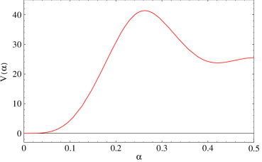
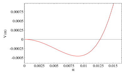
Figure 1: The Higgs potential in the $\delta=0$ set-up, obtained with input parameters $\lambda^{t}=0.99$, $\lambda^{b}=6.9$, $\lambda^{A}=0.24$, $k_{t}=2.42$, $k_{b}=2.26$, $k_{A}=3.14$, $\varepsilon_{1}^{t}=1.9$, $\varepsilon_{2}^{t}=1.6$, $\varepsilon_{1}^{b}=2.9$, $\varepsilon_{2}^{b}=3.4$.

When the bulk-to-boundary couplings are included, the exact spectrum of the bulk-boundary fermion system defined by the Lagrangian (2.5) is determined by solving a complicated transcendental equation (whose form can however be deduced from eqs.(2.15) and (2.16)). The lightest states are identified with the top and bottom quarks and are in general a mixture of localized and bulk fermion states. When the physical mass induced for the boundary fields is much smaller than the masses of the bulk fields, to a very good approximation the top and bottom quark Yukawa couplings (and hence their masses) are found by integrating out the massive bulk fermions and neglecting the momentum dependence induced by higher derivative operators. The relations giving the top and bottom masses are given by appropriate modifications of eqs.(15)-(18) of [9]. One has

$$m_{a}=\left|\frac{m_{0}^{a}}{\sqrt{Z_{1}^{a}Z_{2}^{a}}}\right|\,,\ \ \ a=t,b$$ (2.17)

where

$$m_{0}^{t} = \frac{\epsilon_{1}^{t}\epsilon_{2}^{t}}{\sqrt{2}k_{t}\pi R}\,{\rm Im}\hskip 1.0ptf_{\delta}(\frac{\lambda^{t}}{k_{t}},2\alpha)\;,$$

$$m_{0}^{b} = \frac{\epsilon_{1}^{b}\epsilon_{2}^{b}}{k_{b}\pi R}\,{\rm Im}\hskip 1.0ptf_{\delta}(\frac{\lambda^{b}}{k_{b}},\alpha)\;,$$

$$Z_{i}^{t} = 1+\delta_{i1}\frac{\epsilon_{1}^{b\hskip 1.0pt2}\!}{k_{b}\lambda^{b}}\,{\rm Re}\hskip 1.0ptf_{0}(\frac{\lambda^{b}}{k_{b}},0)+\delta_{i2}\,\frac{\epsilon_{2}^{t\hskip 1.0pt2}\!}{2k_{t}\lambda^{t}}\,{\rm Re}\hskip 1.0ptf_{0}(\frac{\lambda^{t}}{k_{t}},0)+\frac{\epsilon_{i}^{t\hskip 1.0pt2}\!}{2^{\delta_{i2}}k_{t}\lambda^{t}}\,{\rm Re}\hskip 1.0ptf_{0}(\frac{\lambda^{t}}{k_{t}},2\alpha)\;,\qquad$$

$$Z_{i}^{b} = 1+\frac{\epsilon_{i}^{b\hskip 1.0pt2}\!}{k_{b}\lambda^{b}}\,{\rm Re}\hskip 1.0ptf_{0}(\frac{\lambda^{b}}{k_{b}},\alpha)+\delta_{i1}\frac{\epsilon_{1}^{t\hskip 1.0pt2}}{k_{t}\lambda^{t}}\,{\rm Re}\hskip 1.0ptf_{0}(\frac{\lambda^{t}}{k_{t}},\alpha)\;.$$ (2.18)

The changes induced by the $k_{i}$’s are better seen in the limit in which one takes large bulk-to-boundary mixing $\epsilon_{1}^{t},\epsilon_{2}^{t}>>1$ and $\alpha_{min}<<1$. For simplicity, we also take $\epsilon_{1}^{b}=\epsilon_{2}^{b}=0$, since we are mainly interested on the top mass formula. In these approximations one finds

$$m_{t}\simeq\sqrt{2}k_{t}m_{W}F[(2-\delta)\lambda_{t}/k_{t}]\,,$$ (2.19)

where

$$F(x)=\frac{x}{\sinh{x}}\,.$$ (2.20)

The function $F(x)$ has a maximum for $x=0$, where $F(0)=1$, and is monotonically decreasing for $x\geq 0$. Thus

$$m_{t}\lesssim\sqrt{2}k_{t}m_{W}\,,$$ (2.21)

for both $\delta=0$ and $\delta=1$. It is clear from eq.(2.21) that $k_{t}\sim 2$ is enough to get the correct top mass. Another possible way to increase the top mass is obtained by increasing the rank of the $SU(3)$ representation of the bulk fermion which couples to the localized fields. In this way one can get a larger group-theoretical factor multiplying eq.(2.19), at the cost of introducing large representations of SU(3), lowering the Naïve Dimensional Analysis (NDA) estimate of the cut-off.

2.4 Estimate of the cut-off

We estimate the cut-off $\Lambda$ using NDA, as the value at which the first fundamental coupling in the theory gives rise to one-loop diagrams of the same size as the tree–level ones. For simplicity, we consider the non-compact limit $R\rightarrow\infty$, but with $g_{5}/\sqrt{2\pi R}=g$ fixed. The 5D loop factor is $24\pi^{3}$, so one gets

$$\frac{1}{2}\frac{g_{5}^{2}\Lambda}{24\pi^{3}}=\frac{g^{2}\Lambda R}{24\pi^{2}}\simeq 1\,,$$ (2.22)

where the factor 1/2 in the first expression of eq.(2.22) is due to the ${\bf Z}_{2}$ orbifold projection. We should be careful since $g_{5}k$ is effectively a new coupling constant. The most stringent bounds arise indeed from this coupling, when $g_{5}$ is the strong $SU(3)_{c}$ coupling constant. One finds $R\Lambda_{c}\sim 24\pi^{2}/(kg_{s}^{2})\simeq 100/(kR)$, namely that the cut-off scales as $1/k$. This rescaling can easily be understood in the non-compact case, by noting that $k$ enters not only in the coupling, $g_{5}\rightarrow g_{5}k$, but also in the propagators of the virtual states running in the loop. The latter is reabsorbed by sending $q_{5}\rightarrow q_{5}/k$, $q_{5}$ being the momentum along the fifth direction, so that the loop factor scales as $1/k$. We see that NDA does not give strong bounds on the allowed values of $k$, as long as $k\lesssim 10$, which is above the values we have considered. If one takes instead the electroweak coupling constant, $\Lambda_{w}\sim 1000/(kR)$ and no significant constraint arises.

Although $k$ is practically not constrained by perturbativity, it is important to recall that the explicit breaking of the SO(4,1) Lorentz symmetry presents the drawback of generating several counterterms in the effective action which are no longer constrained by SO(4,1) to be absent or equal between each other. This would result in a less constrained model and would also lead to the appearance of additional radiative corrections, absent in the SO(4,1) invariant case. As an example of an effect of this sort, we would expect that at two-loop level the Higgs mass will develop a linear divergence. Indeed, although we think that the Higgs mass term would still be finite, being associated to non-local operators [29], the wave function renormalization of the field $A_{5}$ is no longer exactly cancelled by the gauge coupling constant renormalization, as in the SO(4,1) invariant case, giving rise to a divergence for the physical Higgs mass. Since the Higgs mass term is one-loop induced, such divergence occurs at two-loop level. It is important to stress that this two-loop linear divergence does not significantly destabilize the Higgs mass. It would be interesting to better quantify how higher loop corrections, in general, modify the predictions we have given for the Higgs mass, compactification scale and other parameters.

3 Results

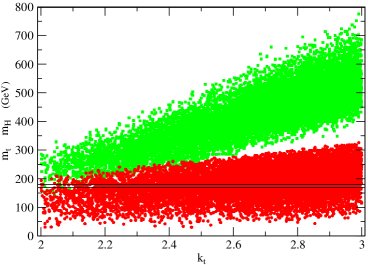
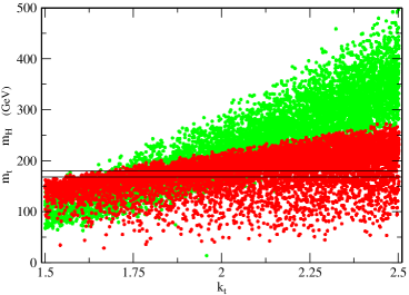
Figure 2: Top (red) and Higgs (green) masses versus the input value of $k_{t}$ for $\delta=0$ (left) and $\delta=1$ (right). The interval between the two black lines corresponds to the physical top mass.

In the present section we report the predictions of our model, as obtained by a numerical study. The analysis is performed by randomly extracting the microscopic parameters within suitable ranges, and computing the resulting values for the relevant observables, namely the Higgs and top masses and the compactification scale. Obviously, we restrict to configurations for which the electroweak symmetry is spontaneously broken, so that we discard points for which $\alpha_{min}=0$. Moreover, a cut $\alpha_{min}<0.05$ is applied in order for the compactification scale $1/R$ to be sufficiently high. As described in section 2, we consider two variants of the model ($\delta=0$ and $\delta=1$) which differ in the location of the boundary fields. The two cases have many qualitative features in common, but they give rise to different quantitative predictions. In particular, different ranges are obtained for the Higgs mass.

3.1 Set-up with $\delta=0$

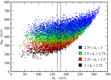
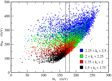
Figure 3: Correlation between Higgs and top masses for $\delta=0$ (left) and $\delta=1$ (right). Different colors label input values of $k_{t}$ in different ranges and the region among the two vertical black lines corresponds to the physical top mass.

As already mentioned, the cancellation of the quadratic term in the effective potential, which permits to obtain small enough values of $\alpha_{min}$, basically results in a correlation between $k_{A}$ and $k_{t}$. Our numerical study reveals indeed acceptable points (with $\alpha_{min}<0.05$) to be only found when $1.1\times k_{t}<k_{A}<1.5\times k_{t}$. For realizing the plots which follows, the bounds

$$\left\{\begin{tabular}[]{l}$2<k_{t}<3$\\ $2<k_{b}<3$\\ $2.6<k_{A}<3.9$\\ \end{tabular}\right.\,,\hskip 30.00005pt\left\{\begin{tabular}[]{l}$0.5<\lambda^{t}<1.5$\\ $5<\lambda^{b}<7$\\ $0.13<\lambda^{A}<3.3$\end{tabular}\right.\,,\hskip 30.00005pt\left\{\begin{tabular}[]{l}$0.75<\epsilon^{t}_{i}<7.5$\\ $2<\epsilon^{b}_{i}<7$\end{tabular}\right.\,,$$

have been used for the input microscopic parameters. First of all, in order to appreciate the effect of the Lorentz violating parameters $k_{i}$, let us see how the various observables depend on $k_{t}$. Clearly, due to the aforementioned cancellation condition, the behaviour in $k_{A}$ is similar to the latter, while the results are weakly sensitive to $k_{b}$ (and to all others $b$ parameters as well), due to the high value of $\lambda^{b}$, which suppresses their contributions. In figure 2, the dependence on $k_{t}$ of the Higgs and top masses is shown. As expected, the upper bound on the top mass linearly increases with $k_{t}$ and correct values (between the black lines in the figure) are obtained for $k_{t}\geq 2$. On the other hand, as expected from eq.(2.14), the Higgs mass grows quadratically with $k_{t}$.

It can be inferred from figure 2 that, at fixed $k_{t}$, a certain correlation between the Higgs and top masses exists. This is shown in fig. 3, in which the Higgs mass is plotted versus the top one, and different colors correspond to different values of $k_{t}$. Figure 4 shows $m_{H}$ and $m_{t}$ as a function of $\alpha_{min}$. Higher Higgs and top masses are favoured at small values of $\alpha_{min}$, even though realistic values of $m_{t}$ can always be obtained. The dependence on $\alpha_{min}$ of the upper bound for the top mass can be derived from eqs.(2.17) and (2.18) in the large $\epsilon$ regime.

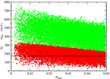
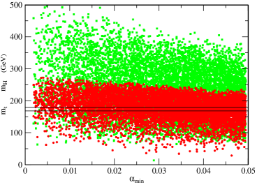
Figure 4: Dependence of the Higgs (green) and top (red) masses on $\alpha_{min}$ for $\delta=0$ (left) and $\delta=1$ (right). The interval between the two black lines corresponds to the physical top mass.

Let us now restrict to realistic values for the top quark mass, in the range $169\;{\rm GeV}<m_{t}<180\;{\rm GeV}$. With this cut (see fig. 5) the Higgs mass is found to be in the range $250-600\ \rm GeV$, independently of the value of $\alpha_{min}$. In figure 6, finally, the mass ($M_{t}=\lambda^{t}/\pi R$) of the lightest non-standard fermions in the model, coming from the KK towers of $\Psi_{t}$ and $\widetilde{\Psi}_{t}$, is plotted versus $\alpha_{min}$. As we will discuss in section 4, this mass is important for estimating new physics effects arising in our model.

3.2 Set-up with $\delta=1$

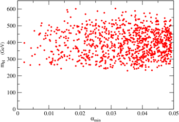
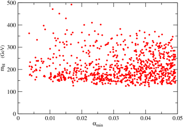
Figure 5: Higgs mass range as a function of $\alpha_{min}$ for $\delta=0$ (left) and $\delta=1$ (right). The top mass has been fixed to the physical value $169\ \rm GeV<m_{t}<180\ \rm GeV$.

As in the case of the previous subsection, acceptable vacua are found only if a certain correlation between $k_{t}$ and $k_{A}$ is imposed. We take $1.1\times k_{t}<k_{A}<1.5\times k_{t}$, and we restrict the other microscopic parameters to the ranges:

$$\left\{\begin{tabular}[]{l}$1.5<k_{t}<2.5$\\ $1.25<k_{b}<2.25$\\ \end{tabular}\right.\,,\hskip 30.00005pt\left\{\begin{tabular}[]{l}$0.5<\lambda^{t}<1.5$\\ $5<\lambda^{b}<7$\\ $0.75<\lambda^{A}<3.5$\end{tabular}\right.\,,\hskip 30.00005pt\left\{\begin{tabular}[]{l}$0.75<\epsilon^{t}_{i}<7.5$\\ $2<\epsilon^{b}_{i}<7$\end{tabular}\right.\,.$$

In figure 2, the dependence on $k_{t}$ of the Higgs and top masses is shown. As in the previous case, the upper bound on the top mass linearly increases with $k_{t}$, while the Higgs mass grows quadratically. Note that, differently from the $\delta=0$ case, configurations with an Higgs mass smaller or equal to the top one can be found (see also figure 3). Figure 4 shows the dependence of the Higgs and top masses on $\alpha_{min}$. The behaviour is similar to the one for $\delta=0$.

We now restrict our analysis to configurations with realistic top mass: $169\ \rm GeV<m_{t}<180\ \rm GeV$. The dependence of the Higgs mass on $\alpha_{min}$ is reported in figure 5. Allowed Higgs masses are in the range $125-400\ \rm GeV$, and the distribution favours small values. Finally, the mass of the lightest non-standard fermions is shown in figure 6. The dependence on $\alpha_{min}$ is analogous to the one found in the case in which all localized fields are at the same fixed point.

3.3 The EW Phase Transition and a Dark Matter Candidate

We have also studied the behaviour of our model at finite temperature, focusing in particular to the study of how (if any) an EW Phase Transition occurs. This analysis is relevant to establish whether baryogenesis at the electroweak scale could be a viable possibility or not. As known, this requires a first-order phase transition where the order parameter $H(T_{C})/T_{C}\geq 1$, $T_{C}$ being the critical temperature of the transition.

The analysis is a simple generalization of [30], so that we will be very brief here and report only the final results. The model develops a first-order phase transition at a temperature of order $T_{C}\sim(0.1-1.5)/(2\pi R)$. We get $0.01\leq H(T_{C})/T_{C}\leq 0.05$ for $\delta=0$ and $0.02\leq H(T_{C})/T_{C}\leq 0.14$ for $\delta=1$. The phase transition strength, as expected, is approximately proportional to $1/m_{H}^{2}$ and this explains why the $\delta=1$ set-up appears to have a stronger phase transition than the $\delta=0$ case. In both cases, however, the latter seems to be too weak to open the possibility of achieving a baryogenesis at the electroweak phase transition.

Interestingly enough, there is a potential DM candidate particle in our model. Thanks to the global $U(1)_{A}$ symmetry that we have imposed to our theory, under which only the antiperiodic fermions transform, the lowest KK modes of both $\Psi_{A}$ and $\widetilde{\Psi}_{A}$ are absolutely stable particles. After EWSB, with the $U(1)^{\prime}$ assignment we have given, the ${\bf 6}$ of $SU(3)_{w}$ gives rise to a couple of four different towers of KK modes (see the appendix of [9] for details), one for $\Psi_{A}$ and one for $\widetilde{\Psi}_{A}$:

$$\begin{array}[]{l@{\hspace{1.5em}}l@{\hspace{1em}}l}\displaystyle m_{n}^{(1)}=\sqrt{\displaystyle M_{A}^{2}+\frac{k_{A}^{2}(n+1/2+\alpha)^{2}}{R^{2}}}\,,\hfil\hskip 15.00002pt&{\rm with}\ \ q=+1\,,\hfil\hskip 10.00002pt&n\in[-\infty,+\infty]\,,\\ \rule{0.0pt}{25.00003pt}\displaystyle m_{n}^{(2)}=\sqrt{\displaystyle M_{A}^{2}+\frac{k_{A}^{2}(n+1/2+2\alpha)^{2}}{R^{2}}}\,,\hfil\hskip 15.00002pt&{\rm with}\ \ q=0\,,\hfil\hskip 10.00002pt&n\in[-\infty,+\infty]\,,\\ \rule{0.0pt}{25.00003pt}\displaystyle m_{n}^{(3)}=\sqrt{\displaystyle M_{A}^{2}+\frac{k_{A}^{2}(n+1/2)^{2}}{R^{2}}}\,,\hfil\hskip 15.00002pt&{\rm with}\ \ q=+2\,,\hfil\hskip 10.00002pt&n\in[0,+\infty]\,,\\ \rule{0.0pt}{25.00003pt}\displaystyle m_{n}^{(4)}=\sqrt{\displaystyle M_{A}^{2}+\frac{k_{A}^{2}(n+1/2)^{2}}{R^{2}}}\,,\hfil\hskip 15.00002pt&{\rm with}\ \ q=0\,,\hfil\hskip 10.00002pt&n\in[0,+\infty]\,,\end{array}$$ (3.1)

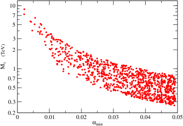
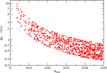
Figure 6: The mass $M_{t}$ of the first non-standard fermions, as a function of $\alpha_{min}$ for $\delta=0$ (left) and $\delta=1$ (right). The top mass has been fixed to the physical value $169\ \rm GeV<m_{t}<\ \rm 180GeV$.

where $q$ is the electromagnetic $U(1)$ charge of the state. The lightest particles in eq.(3.1) are a couple of neutral states with mass $m_{DM}=\sqrt{M_{A}^{2}+k_{A}^{2}(1-4\alpha)^{2}/(4R^{2})}$. Since $m_{DM}\geq 1/R$ for the typical input values of $M_{A}$ and $k_{A}$, which corresponds to a mass of several TeV, such states are potential candidates to explain the observed DM abundance in the Universe.

4 Estimate of Phenomenological Bounds

In this section we give an order–of–magnitude estimate of the main physical effects which we believe to provide the most stringent bounds on our model. The purpose of this analysis is to show that it is not trivially ruled out and to roughly estimate the allowed range in the parameter space of the model.

4.1 Direct Corrections: the $Zb_{L}\bar{b}_{L}$ vertex and FCNC

The first effect one should worry about is the non–universality of the EW couplings which is present in our model, after EWSB, since the physical SM fermions (with diagonal propagators) are a complicated mixture of fields in different representations of the underlying 5D $SU(3)_{w}$ EW group. The $e_{i}^{t,b}$ couplings in Eq. (2.5), indeed, make the localized fields $Q_{L}$ and $b_{R},t_{R}$ to mix with the Kaluza–Klein towers of $\Psi_{t,b}$ and $\tilde{\Psi}_{t,b}$ in the ${\bf 6}$ and ${\bf 3}$ representations of $SU(3)$, which contain singlets, doublets and triplets of $SU(2)_{w}$. Due to gauge invariance, the localized fields only couple to the components of the bulk ones with the right (${\bf 2}_{1/6}$, ${\bf 1}_{-1/3}$ and ${\bf 1}_{2/3}$) quantum numbers. After EWSB, however, mixing among fields in different representations are generated. The latter give rise to tree–level corrections to the EW couplings through tree–level diagrams such as in fig. 7, in which all standard and non–standard fermions ${q^{\prime}}_{n}$, belonging to the Kaluza–Klein towers of $\Psi$, $\tilde{\Psi}$, propagate. The couplings of ${q^{\prime}}_{n}$ to the SM gauge bosons is diagonal, since the wave function of the latter in the extra dimension is flat. We focus in the following only on the corrections to the vertex of the $Z$ gauge boson, since this is the one which is experimentally more constrained. Diagrams such as the one depicted in fig. 7 give rise at the same time to a vertex and a propagator correction. The physical correction to the vertex is obtained only after having canonically normalized the kinetic terms for the external SM fermions. Gauge invariance allows Yukawa couplings of the SM Higgs and the bottom quark $b_{L}$ only through triplets of $SU(2)$, arising from the ${\bf 6}$ of $SU(3)_{w}$.

Figure 7: The leading tree–level correction to the $Zb_{L}\bar{b}_{L}$ vertex and to the $b_{L}$ propagator. The distortion of the $Zb_{L}\bar{b}_{L}$ coupling is generated through the Higgs–mediated mixing of $b_{L}$ with one component ($\phi_{3}$) of the ${\bf 3}_{1/3}$ triplet contained in $\Psi_{t}$.

As it is clear from fig. 7, the distortion is inversely proportional to the mass of the triplets and proportional to the mixing between the doublet and the triplet. Computing the overlap of the wave functions of the quark doublet with all the KK tower of the triplets and then diagonalizing the resulting mass matrix is not straightforward. To a very good approximation, however, the distortion is dominated by the first massive state of the KK tower, with mass $M_{t}$. This is not only the lightest state of the tower, but also the one which mixes more with the quark doublet. By considering only such a state, an explicit computation shows that for the down quarks one has

$$\frac{\delta g_{b}}{g_{b}}\simeq\frac{1}{1-\frac{2}{3}\sin^{2}\theta_{W}}\frac{\epsilon_{1}^{t\,2}k_{t}^{2}}{\lambda^{t\,2}Z_{1}}\Big{(}\frac{m_{W}}{M_{t}}\Big{)}^{2}\,,$$ (4.1)

where $Z_{1}$ is the factor appearing in eq.(2.18), evaluated at $\alpha=0$, for which $Z_{1}=Z_{1}^{t}=Z_{1}^{b}$. We expect that a similar estimate will also apply for up quarks. The distortion caused by eq.(4.1) is always safely below current experimental bounds for all light quarks (including all leptons), in which the bulk fermions are very massive and/or one can consider moderately small mixing $\epsilon_{1}^{u}\lesssim 0.1$. The only exception is represented by the bottom quark, because the requirement of getting a reasonable mass for the top quark obliges us to take $\epsilon_{1}^{t}\geq 1$ and $\lambda^{t}\sim 1$. It turns out, indeed, that eq.(4.1) represents a strong constraint on the parameter space of the model, as can be seen from figure 12, where $\delta g_{b}/g_{b}$ is reported as a function of $\alpha_{min}$, the most relevant parameter. Considering that $(\delta g_{b}/g_{b})_{exp}\leq 10^{-2}-10^{-3}$, essentially all values of $\alpha_{min}\geq 2\times 10^{-2}$ ($1/R\lesssim$ 4 TeV) are ruled out. It is interesting to notice that the constraint imposed by $Zb_{L}\bar{b}_{L}$ also plays an important role in the warped model of [14, 31]. In the latter case, as in ours, the requirement of having an acceptable top mass forbids to lower this distortion.

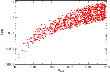
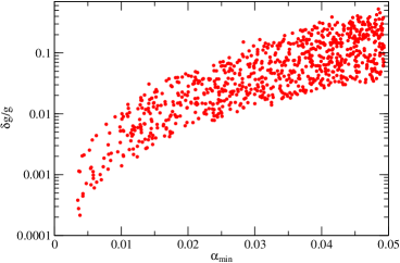
Figure 8: Correction to the $Zb_{L}\bar{b}_{L}$ coupling $\delta g_{b}/g_{b}$ as a function of $\alpha_{min}$ for $\delta=0$ (left) and $\delta=1$ (right).

Another important issue to consider, closely related to the non–universality of the EW couplings, is the suppression of the FCNC which are typically generated at tree–level when integrating out the massive KK modes. For simplicity, consider here the case in which the bulk-to-boundary couplings $\epsilon_{i}$ are diagonal in flavour space and the non-trivial flavour structure, as in [9], is totally encoded in non-trivial bulk mass matrices, which can now involve not only the bulk mass terms $M_{i}$ but also the Lorentz violating factors $k_{i}$. The FCNC are induced in our model by tree-level couplings which arise from diagrams such as the one in fig. 7, in which the non-standard triplet $\phi_{3}$ switches at some point to the KK mode of a different family. Their structure can then be inferred from eq.(4.1), which is in fact the leading correction to a flavour preserving neutral current or to a FCNC, modulo the flavour textures which we will not specify here and conservatively take to be of order one. The typical bound on the couplings of FCNC involving $b$ quarks is $\lesssim 10^{-2}$. Since these couplings are equal to or smaller than the value estimated by eq.(4.1), they do not represent any problem. In other words, the strongest bounds in $b$-physics arise from the $Zb_{L}\bar{b}_{L}$ correction.

The bounds on the couplings of FCNC involving $d$ and $s$ quarks are instead much stronger, $\lesssim 10^{-5}$. In particular, one should worry that, in presence of a generic flavour mixing, a light quark ($d$ or $s$) can first switch to a triplet of the heavy KK tower of the bulk fermion of the corresponding up quark ($u$ or $c$), which then switches to the much lighter triplet of the KK tower of the top quark. The latter emits a $Z$ boson and then switches to another heavy KK tower and thus eventually to another light quark ($s$ or $d$), resulting in a FCNC. We can estimate the tree–level coupling $g_{FCNC}$ of this FCNC vertex from eq.(4.1). Neglecting the factor $Z_{1}$, which is typically of order 1, one has

$$g_{FCNC}\sim\frac{\epsilon_{1}^{c}\epsilon_{1}^{u}}{\lambda^{c}\lambda^{u}}\Big{(}\frac{m_{W}}{M_{t}}\Big{)}^{2}\,.$$ (4.2)

Considering that for the $c$ and the $u$ quarks one can take $\lambda^{c}\lambda^{u}\gtrsim 10$ and, at the same time, one can naturally take $\epsilon_{1}^{u,c}\sim 0.1$, it is reasonable to expect that $g_{FCNC}$ can be made smaller than $10^{-5}$ or $10^{-6}$.

FCNC are also induced by the exchange of the massive KK modes of the $Z$ gauge boson and gluons [32], due to the non–universality of their couplings to different families. This effect, which is present even in the absence of EWSB, comes from the fact that in our model, as required for explaining the mass hierarchy, quarks of different families have different wave functions. By choosing for different generations the same distribution of localized fields, we can however strongly suppress this effect. Flavour non–universality in the KK couplings, indeed, arises in this case only from diagrams in which the brane quark $q$ is changed to a bulk KK fermion, which emits a KK gauge boson, and then back to the brane. The effective coupling of this diagram can be estimated as

$$\frac{\delta g_{KK}}{g_{KK}}\sim\frac{{\epsilon^{q}}^{2}}{\lambda^{q\,2}}\,.$$ (4.3)

For the light families, if $\epsilon^{q}$ is moderately small ($\lesssim 10^{-1}$), we expect the coupling (4.3) to be naturally of order of $10^{-3}-10^{-4}$, since $\lambda^{q\,2}\gtrsim 10$. In this way, the resulting FCNC — due to their stronger couplings, gluons give the dominant contribution — is of the same order of magnitude of that estimated for the $Z$ and thus within the current limits.

4.2 Oblique Corrections: $\Delta\rho$

Figure 9: Leading tree-level correction to $\Delta\rho$.

The leading worrisome universal deviation from the SM in our theory is due to the localized mass terms for the gauge field $A_{X}$, which are necessarily present, as explained in subsection 2.2, for anomaly cancellation. They induce tree-level mixing between the $Z$ boson and the KK modes of $A_{X}$, which are conveniently expressed in the following term:

$${\mathcal{L}}_{m}=\frac{1}{2\cos^{2}\theta_{W}}\frac{\alpha^{2}}{R^{2}}\Big{(}Z-\sqrt{3-4\sin^{2}\theta_{W}}A_{X}(y)\Big{)}^{2}\,,$$ (4.4)

where $Z=\cos\theta_{W}A^{3}_{0}-\sin\theta_{W}A_{Y,0}$ is the usual 4D SM gauge boson, whereas $A_{X}(y)$ is the 5D field in eq.(2.6). Since, due to the anomaly, the wave functions (2.6) are not regular cosines, the $A_{X,\,n}$ fields couple to the zero–mode of the $Z$ via the $Z$–$A_{X}$ term in eq. (4.4), see also fig. 9. The physical mass eigenstate of the $Z$, given by eq.(2.8), is then a complicated mixture of the full KK towers of $A_{X}$, which lead to a deviation from the SM relation $m_{Z}=m_{W}/\cos\theta_{W}$ or $\rho=1$. The deviation $\Delta\rho=\rho-1$ (or $T$) is easily computed by expanding in series the sines in eq.(2.8), or diagrammatically, by considering the $Z$–$A_{X}$ mixing terms in eq.(4.4). The result is

$$\Delta\rho=\frac{8\pi^{2}}{9(1+3\delta)}\alpha_{min}^{2}+O(\alpha_{min}^{4})\,.$$ (4.5)

The current experimental limit on $\Delta\rho$ is $\Delta\rho_{exp}\lesssim 10^{-3}$, so that eq.(4.5) leads to a bound on $\alpha_{min}$ which is $\alpha_{min}\lesssim 10^{-2}$ ($1/R\gtrsim 8$ TeV) for $\delta=0$ and $\alpha_{min}\lesssim 2\times 10^{-2}$ ($1/R\gtrsim 4$ TeV) for $\delta=1$. For $\delta=0$, eq.(4.5) represents the strongest bound on the model, whereas for $\delta=1$ it equals the bound found in the last subsection from $Zb\bar{b}$.

We have not computed the corrections induced by four fermion operators, since we expect that the associated bounds in our model are roughly the same as the ones estimated in [19] for universal theories in which the gauge and Higgs field are bulk fields and the SM fermions are localized states. As such, the resulting bound on $1/R$ is approximately the same as the one coming from $Zb_{L}\bar{b}_{L}$ or $\Delta\rho$. Other universal corrections arise at one-loop level. The leading ones are given by vector-like massive Dirac fermions and are safely small.

4.3 The Fine–Tuning

The phenomenological bounds estimated before essentially result in a bound on $\alpha_{min}$ which is $\alpha_{min}\sim 10^{-2}$. As can be seen from, say, figure 5, low values of $\alpha_{min}$ are not so uncommonly obtained. It is however important to better quantify how much fine-tuning is necessary to impose in the microscopic parameters of our theory to get $\alpha_{min}\sim 10^{-2}$. The exact determination of such tuning is actually a very challenging task due to the difficulty of choosing a precise definition of the tuning itself.

The fine-tuning, according to a commonly used definition [34], is related to the sensitivity of the physical observables to the microscopic parameters of the theory. In such a view, the fine-tuning can be estimated by computing the logarithmic derivative of the observables with respect to the parameters. In our case the most sensitive observable is the Higgs VEV (namely $\alpha_{min}$), while the most relevant parameters are the Lorentz violating couplings $k_{t}$ and $k_{A}$ or, better, their ratio $\beta=k_{A}/k_{t}$. Computing the derivative

$$C(\beta)\equiv\frac{\partial\log\alpha_{min}}{\partial\log\beta}\,,$$ (4.6)

one finds $C\sim 10^{3}$ for $\alpha_{min}\sim 10^{-2}$. If one takes $1/C$ as an estimate of fine-tuning in the model, this should translate in a fine-tuning of ${\cal O}(\kern-0.50003pt\raise 2.15277pt\hbox{\sevenrm0}\kern-1.49994pt/\kern-1.49994pt\lower 1.07639pt\hbox{\sevenrm00})$.

In [35], an improved definition of fine-tuning was proposed. According to this prescription, the value of the logarithmic derivative $C(\beta)$ at a given point must be divided by the average value of $C$ in a suitable range of the microscopic parameters. This should allow to distinguish “spurious” high sensitivity to the parameters from “real” fine-tuning due to cancellations. In this procedure, however, an appropriate definition of the range of the microscopic parameters, in which the average will be performed, must be chosen. In the present case, the result crucially depends on what we assume to be the “natural” values of $\beta$, i.e. on what we decide to be its “natural” interval of variation. If we take values of $\beta$ for which the EWSB is realized (roughly $0\lesssim\beta\lesssim 1$), i.e. all values for which $0<\alpha_{min}<1/2$, and average over all the resulting vacua, the fine-tuning turns out to be roughly as before of ${\cal O}(\kern-0.50003pt\raise 2.15277pt\hbox{\sevenrm0}\kern-1.49994pt/\kern-1.49994pt\lower 1.07639pt\hbox{\sevenrm00})$.

However, we notice that most of the vacua in this ensemble are either at $\alpha_{min}=0$ or at large values $\alpha_{min}\sim 1/3$. If one disregards these points, by taking for instance a range of $\beta$ for which $0<\alpha_{min}<1/4$, one finds a relevant “spurious” sensitivity of $\alpha_{min}$ on $\beta$. The range of $\beta$ for which $0<\alpha_{min}<1/4$ is quite small and the “real” fine-tuning is found now, applying the proposal of [35], to be of ${\cal O}(10\%)$.

Although it is hard to draw a conclusion about the fine-tuning in our model, in the light of these different estimates, we think that it might be fair to say that the bound $\alpha_{min}\sim 10^{-2}$ could be translated to a fine-tuning of ${\cal O}(\%)$.

5 Is Our Model Really a 5D Theory ?

In this work we have essentially shown how it is possible to get a potentially realistic model with gauge-Higgs unification at the price of explicitly breaking the SO(4,1)/SO(3,1) Lorentz generators in the fermionic sector. In light of this breaking, one could wonder whether it is correct to consider our model as a “canonical” 5D theory or not. Indeed, contrary to the usual “spontaneous” breaking of the SO(4,1)/SO(3,1) Lorentz symmetry induced by the compactification, which implies that at short distances $\Delta x\ll R$ the model is effectively a 5D Lorentz invariant theory (in the bulk), the explicit breaking we advocate implies that at arbitrarily short scales the SO(4,1) symmetry is not recovered. This is clearly a theoretical issue, which is mainly related to the possible existence and form of an underlying UV completion of our model. Moreover, the concept of gauge-Higgs unification itself relies on the existence of a 5D interpretation. It is clear that we can always consider our model as an IR effective description of a 4D moose theory for which the “accidental” SO(4,1) Lorentz symmetry is not recovered in the fermionic sector [8]. From this point of view, our model would resemble more a moose-based little Higgs model rather than a gauge-Higgs unification model. We would like to point out, however, that the SO(4,1) Lorentz breaking we advocate in this paper can have a simple origin in the context of a purely 5D theory. A particularly elegant and interesting explanation is the following. Consider an axion-like field $\Phi$, which for simplicity we take to be dimensionless, invariant under the shift $\Phi\rightarrow\Phi+2\pi$. In light of this shift symmetry, one can take twisted periodicity conditions for $\Phi$, which reads

$$\Phi(y+2\pi R)=\Phi(y)+2\pi\,.$$ (5.1)

Scherk-Schwarz reductions of the form (5.1) are not new, appearing in Supergravity as a way to obtain gauged SUGRA or theories with fluxes (see e.g. [36]). Consistency of eq.(5.1) with the ${\bf Z}_{2}$ orbifold action $y\rightarrow-y$ requires that $\Phi$ should be ${\bf Z}_{2}$ odd. This is welcome, implying that all the excitations of $\Phi$ are massive. Due to the twisted condition (5.1), the VEV of $\Phi$ is non-trivial. The background configuration $\Phi_{0}$ which satisfies the field equations of motion and eq.(5.1) is

$$\Phi_{0}(y)=\frac{y}{R}\,,$$ (5.2)

which clearly induces a spontaneous breaking of the SO(4,1)/SO(3,1) Lorentz symmetry. The Lorentz violating factors $k$ introduced in eq.(2.5) are then reinterpreted as due to couplings involving $\Phi$ and fermion bilinears. It turns out that if we also impose a ${\bf Z}_{2}$ global symmetry under which $\Phi\rightarrow-\Phi$, the lowest dimensional operator which couples $\Phi$ and bulk fermions read

$$\frac{\gamma}{f_{\Phi}^{2}}\partial_{M}\Phi\partial_{N}\Phi\overline{\Psi}\gamma^{M}D^{N}\Psi\,,$$ (5.3)

where $\gamma$ is a dimensionless coupling and $f_{\Phi}$ is the “$\Phi$ decay constant”. When $\langle\Phi\rangle=\Phi_{0}$, the operator (5.3) precisely induces the Lorentz violating terms which appear in the Lagrangian (2.5). Since we have considered in our model values of $k$ which are not close to 1, the effective coupling constant of the operator (5.3) is strong (of order 1) and thus insertions of this operator have to be resummed. This is what we have effectively done in our previous analyses. Notice that eq.(5.2) can also be interpreted as a non-vanishing flux for the 1-form field-strength $H_{1}=d\Phi\sim dy$ or else for a non-vanishing flux for the Hodge dual 4-form field-strength $H_{4}\sim dx^{0}\wedge dx^{1}\wedge dx^{2}\wedge dx^{3}$.

We think that the above picture — in no way necessary for the model we have presented — shows that the Lorentz violating factors $k_{j}$ can have a natural origin in a 5D framework.

In light of the rescaling (2.13), the factors $k_{j}$ effectively imply that different fermions “see” a different radius of compactification. Their effect is then quite similar to recent ideas in the context of Higgless models in 5D warped models, in which it has been advocated that different fields could propagate in internal spaces with different sizes [37, 38].

6 Outlook

In this paper we have shown that realistic models based on gauge-Higgs unification in 5D flat space can be constructed, but at the price of breaking the SO(4,1) Lorentz symmetry in the bulk. Our key observation is that the stability of the Higgs potential is mostly provided by the 5D gauge symmetry rather than the SO(4,1) symmetry. Breaking the latter results in additional divergencies and in an increasing number of independent operators to be considered, which however do not significantly destabilize the Higgs potential. Somehow, the SO(4,1) breaking models we propose represent a sort of middle course between little Higgs models and the previously considered SO(4,1) invariant models with gauge-Higgs unification. For simplicity, we have focused our attention on a variant of the minimal model of [9], where an additional antiperiodic bulk fermion is introduced. The latter state is crucial to increase the value of the compactification scale above the TeV scale and, as a by product, its lightest neutral KK state is a possible DM candidate. Clearly, several other models, already constructed or not, could be considered in this Lorentz non-invariant scenario. We have also shown that our model could pass various phenomenological tests, such as the universality of the couplings, EWPT and FCNC.

An important issue that we have not considered at all in this paper regards the experimental signatures of our model. In the light of the forthcoming Large Hadron Collider (LHC), it is particularly important to address which are (if any) the distinct collider signatures of our model. We plan to address in a future work the latter issue, as well as a detailed study of the viability of our theory as a realistic proposal to go beyond the SM.

References

- [1]
- [2] I. Antoniadis, Phys. Lett. B 246 (1990) 377.
-
[3]
G. R. Dvali, S. Randjbar-Daemi, R. Tabbash,
Phys. Rev. D 65 (2002) 064021
[hep-ph/0102307];
L. J. Hall, Y. Nomura, D. R. Smith, Nucl. Phys. B 639 (2002) 307 [hep-ph/0107331];
I. Antoniadis, K. Benakli, M. Quiros, New J. Phys. 3 (2001) 20 [hep-th/0108005];
M. Kubo, C. S. Lim and H. Yamashita, Mod. Phys. Lett. A 17 (2002) 2249 [arXiv:hep-ph/0111327];
N. Haba, M. Harada, Y. Hosotani and Y. Kawamura, Nucl. Phys. B 657 (2003) 169 [Erratum-ibid. B 669 (2003) 381] [arXiv:hep-ph/0212035];
N. Haba, Y. Shimizu, Phys. Rev. D 67 (2003) 095001 [hep-ph/0212166];
K. w. Choi et al., JHEP 0402 (2004) 037 [arXiv:hep-ph/0312178];
I. Gogoladze, Y. Mimura, S. Nandi, Phys. Lett. B 560 (2003) 204 [hep-ph/0301014];
ibid. 562 (2003) 307 [hep-ph/0302176]; Phys. Rev. D 69 (2004) 075006; [arXiv:hep-ph/0311127].
C. A. Scrucca, M. Serone, L. Silvestrini and A. Wulzer, JHEP 0402 (2004) 049 [arXiv:hep-th/0312267]; A. Wulzer, “Gauge-Higgs unification in six dimensions,” arXiv:hep-th/0405168.
C. Biggio and M. Quiros, Nucl. Phys. B 703 (2004) 199 [arXiv:hep-ph/0407348]. - [4] G. Burdman, Y. Nomura, Nucl. Phys. B 656 (2003) 3 [hep-ph/0210257].
-
[5]
D. B. Fairlie,
Phys. Lett. B 82 (1979) 97;
J. Phys. G 5 (1979) L55;
N. S. Manton, Nucl. Phys. B 158 (1979) 141;
P. Forgacs, N. S. Manton, Commun. Math. Phys. 72 (1980) 15;
S. Randjbar-Daemi, A. Salam, J. Strathdee, Nucl. Phys. B 214 (1983) 491;
N. V. Krasnikov, Phys. Lett. B 273 (1991) 246;
H. Hatanaka, T. Inami, C. Lim, Mod. Phys. Lett. A 13 (1998) 2601 [hep-th/9805067]. - [6] M. Serone, AIP Conf. Proc. 794 (2005) 139 [arXiv:hep-ph/0508019].
-
[7]
N. Arkani-Hamed et al.,
JHEP 0208 (2002) 021
[arXiv:hep-ph/0206020];
N. Arkani-Hamed, A. G. Cohen, E. Katz and A. E. Nelson, JHEP 0207 (2002) 034 [arXiv:hep-ph/0206021]. - [8] N. Arkani-Hamed, A. G. Cohen and H. Georgi, Phys. Lett. B 513 (2001) 232 [arXiv:hep-ph/0105239].
- [9] C. A. Scrucca, M. Serone, L. Silvestrini, Nucl. Phys. B 669 (2003) 128 [hep-ph/0304220].
- [10] C. Csaki, C. Grojean, H. Murayama, Phys. Rev. D 67 (2003) 085012 [hep-ph/0210133].
-
[11]
Y. Grossman and M. Neubert,
Phys. Lett. B 474 (2000) 361
[arXiv:hep-ph/9912408];
T. Gherghetta and A. Pomarol, Nucl. Phys. B 586 (2000) 141 [arXiv:hep-ph/0003129]. - [12] N. Arkani-Hamed and M. Schmaltz, Phys. Rev. D 61 (2000) 033005 [arXiv:hep-ph/9903417].
-
[13]
R. Contino, Y. Nomura and A. Pomarol,
Nucl. Phys. B 671 (2003) 148
[arXiv:hep-ph/0306259];
K. y. Oda and A. Weiler, Phys. Lett. B 606 (2005) 408 [arXiv:hep-ph/0410061];
Y. Hosotani and M. Mabe, Phys. Lett. B 615 (2005) 257 [arXiv:hep-ph/0503020]. - [14] K. Agashe, R. Contino and A. Pomarol, Nucl. Phys. B 719 (2005) 165 [arXiv:hep-ph/0412089].
- [15] G. Cacciapaglia, C. Csaki and S. C. Park, “Fully radiative electroweak symmetry breaking,” arXiv:hep-ph/0510366.
- [16] G. Servant and T. M. P. Tait, Nucl. Phys. B 650 (2003) 391 [arXiv:hep-ph/0206071].
- [17] K. Agashe, A. Delgado, M. J. May and R. Sundrum, JHEP 0308 (2003) 050 [arXiv:hep-ph/0308036].
-
[18]
G. Burdman and Y. Nomura,
Phys. Rev. D 69 (2004) 115013
[arXiv:hep-ph/0312247];
G. Cacciapaglia, C. Csaki, C. Grojean and J. Terning, Phys. Rev. D 71 (2005) 035015 [arXiv:hep-ph/0409126]. - [19] R. Barbieri, A. Pomarol, R. Rattazzi and A. Strumia, Nucl. Phys. B 703, 127 (2004) [arXiv:hep-ph/0405040].
- [20] J. Scherk and J. H. Schwarz, Phys. Lett. B 82 (1979) 60; Nucl. Phys. B 153 (1979) 61.
- [21] Y. Hosotani, Phys. Lett. B 126 (1983) 309; ibid. 129 (1983) 193; Ann. Phys. 190 (1989) 233.
- [22] M. Serone and A. Wulzer, Class. Quant. Grav. 22 (2005) 4621 [arXiv:hep-th/0409229]; A. Wulzer, “Orbifold resolutions with general profile,” arXiv:hep-th/0506210.
- [23] G. Martinelli, M. Salvatori, C. A. Scrucca and L. Silvestrini, JHEP 0510 (2005) 037 [arXiv:hep-ph/0503179].
-
[24]
C. A. Scrucca, M. Serone, L. Silvestrini, F. Zwirner,
Phys. Lett. B 525 (2002) 169
[hep-th/0110073];
L. Pilo, A. Riotto, Phys. Lett. B 546 (2002) 135 [hep-th/0202144];
R. Barbieri, R. Contino, P. Creminelli, R. Rattazzi, C. A. Scrucca, Phys. Rev. D 66 (2002) 024025 [hep-th/0203039];
C. A. Scrucca, M. Serone and M. Trapletti, Nucl. Phys. B635, 33 (2002) [hep-th/0203190]. -
[25]
M. B. Green, J. H. Schwarz,
Phys. Lett. B 149 (1984) 117;
E. Witten, Phys. Lett. B 149 (1984) 351;
M. Dine, N. Seiberg, E. Witten, Nucl. Phys. B 289 (1987) 589. - [26] G. von Gersdorff, N. Irges and M. Quiros, Nucl. Phys. B 635 (2002) 127 [arXiv:hep-th/0204223]; “Finite mass corrections in orbifold gauge theories,” arXiv:hep-ph/0206029.
- [27] G. Cacciapaglia, talk given at “The 13th International Conference on Supersymmetry and Unification of Fundamental Interactions”, July 18-23, 2005, IPPP Durham.
- [28] N. Haba, Y. Hosotani, Y. Kawamura and T. Yamashita, Phys. Rev. D 70 (2004) 015010 [arXiv:hep-ph/0401183].
-
[29]
N. Arkani-Hamed et al.,
Nucl. Phys. B605 (2001) 81
[hep-ph/0102090];
A. Masiero, C. A. Scrucca, M. Serone, L. Silvestrini, Phys. Rev. Lett. 87 (2001) 251601 [hep-ph/0107201]. - [30] G. Panico and M. Serone, JHEP 0505 (2005) 024 [arXiv:hep-ph/0502255].
- [31] K. Agashe and R. Contino, “The Minimal Composite Higgs Model and Electroweak Precision Tests,” arXiv:hep-ph/0510164.
- [32] A. Delgado, A. Pomarol and M. Quiros, JHEP 0001 (2000) 030 [arXiv:hep-ph/9911252].
- [33] M. E. Peskin and T. Takeuchi, Phys. Rev. D 46 (1992) 381.
- [34] R. Barbieri and G. F. Giudice, Nucl. Phys. B 306 (1988) 63.
- [35] G. W. Anderson and D. J. Castano, Phys. Lett. B 347 (1995) 300 [arXiv:hep-ph/9409419].
- [36] E. Bergshoeff et al., Nucl. Phys. B 470 (1996) 113 [arXiv:hep-th/9601150].
- [37] G. Cacciapaglia et al., “Top and bottom: A brane of their own,” arXiv:hep-ph/0505001.
- [38] R. Foadi and C. Schmidt, “An effective Higgsless theory: Satisfying electroweak constraints and a heavy top quark,” arXiv:hep-ph/0509071.