HEPHY-PUB 812/05 hep-ph/0510372 October 2005

EXACT-PROPAGATOR INSTANTANEOUS BETHE–SALPETER EQUATION FOR QUARK–ANTIQUARK BOUND STATES
LI Zhi-Feng
Institut für Theoretische Physik, Universität Wien,
Boltzmanngasse 5, A-1090 Wien, Austria
Wolfgang LUCHA
Institut für Hochenergiephysik,
Österreichische Akademie der Wissenschaften,
Nikolsdorfergasse 18, A-1050 Wien, Austria
Franz F. SCHÖBERL
Institut für Theoretische Physik, Universität Wien,
Boltzmanngasse 5, A-1090 Wien, AustriaAbstract

Recently an instantaneous approximation to the Bethe–Salpeter formalism for the analysis of bound states in quantum field theory has been proposed which retains, in contrast to the Salpeter equation, as far as possible the exact propagators of the bound-state constituents, extracted nonperturbatively from Dyson–Schwinger equations or lattice gauge theory. The implications of this improvement for the solutions of this bound-state equation, that is, the spectrum of the mass eigenvalues of its bound states and the corresponding wave functions, when considering the quark propagators arising in quantum chromodynamics are explored. PACS numbers: 11.10.St, 03.65.Ge, 03.65.Pm

1 Introduction

The more than half a century old Bethe–Salpeter formalism[1] constitutes a relativistically covariant framework within the realms of quantum field theory for the description of bound states from first principles. The Bethe–Salpeter equation controls a bound-state amplitude encoding, in momentum space, the distribution of the relative momenta of the bound-state constituents. Within elementary particle physics this formalism has been widely applied to quantum electrodynamics (QED) and quantum chromodynamics (QCD). Unfortunately it faces problems of interpretation and of our ignorance of the full interaction kernel in QCD.

Thus, simplifications of the Bethe–Salpeter equation in form of some three-dimensional reductions are highly desirable. The most famous among all proposals is known as Salpeter equation[2]. Its formulation, however, is based on assuming all bound-state constituents to interact instantaneously and to propagate as free particles; the latter circumstance renders hard to implement effects such as spontaneous chiral-symmetry breaking, crucial for QCD.

In view of this, an instantaneous Bethe–Salpeter equation which incorporates the exact form of the propagators of the bound-state constituents (to the utmost conceivable extent) has been derived recently[3]; this improved bound-state equation reduces, of course, to the Salpeter equation, upon approximation of the exact propagators by their free counterparts. For any description of hadrons as bound states, the exact quark propagators conforming to the QCD Dyson–Schwinger equations are relevant. This work is devoted to the study of the consequences of introducing exact quark propagators in this instantaneous Bethe–Salpeter equation. The most dramatic effect observed is a significant diminution of the level spacing.

The paper is organized as follows. Section 2 sketches the derivation of our instantaneous Bethe–Salpeter equation with exact propagators of the bound-state constituents presented in Ref.[3]. Approximating all interactions entering in the Bethe–Salpeter equation by their static forms but retaining, as far as possible, exact propagators yields[3] a generalization of Salpeter’s equation[2], with momentum-dependent masses of the bound-state constituents and with normalization factors of their exact propagators multiplying all interaction terms. Section 3 introduces the exact light-quark propagators obtained within QCD as solution of the Dyson–Schwinger equations. This infinite tower of coupled integral equations calls for a truncation[4, 5, 6, 7, 8, 9, 10, 11, 12, 13, 14, 15, 16, 17, 18, 19, 20, 21, 22, 23, 24] which must not be in conflict with the relevant Ward–Takahashi identity. Section 4 summarizes the technique developed for finding the solutions of an instantaneous Bethe–Salpeter equation by first reducing it to a coupled set of radial equations[25, 26, 27, 28] and then converting it to a matrix eigenvalue problem[29, 30, 31, 32]. Some implications of taking into account exact instead of free propagators of bound-state constituents are analyzed in Sec. 5 by application of the entire formalism to a linear confining interaction. Section 6 scrutinizes our findings. Appendix A recalls the Hilbert-space basis required for the matrix conversion.

2 Instantaneous Bethe–Salpeter equation with exact propagators

The derivation of the exact-propagator instantaneous Bethe–Salpeter equation[3] parallels the (three-dimensional) reduction of the Bethe–Salpeter equation[1] to the free-propagator Salpeter equation[2]. It may be achieved by several slightly different but equivalent routes.

In the framework of the Bethe–Salpeter formalism, a bound state $|{\rm B}(P)\rangle$ of momentum $P$ and mass $M_{\rm B},$ composed of a fermion and an antifermion described by the field operators $\psi_{1}(x_{1}),$ $\bar{\psi}_{2}(x_{2}),$ resp., is represented, in momentum space, by the Bethe–Salpeter amplitude

$$\Psi(p)\equiv\exp({\rm i}\,P\,X)\int{\rm d}^{4}x\,\exp({\rm i}\,p\,x)\,\langle 0|{\rm T}(\psi_{1}(x_{1})\,\bar{\psi}_{2}(x_{2}))|{\rm B}(P)\rangle\ .$$

Here, $X$ and $x$ denote the center-of-momentum and relative coordinates of the two-particle system while $P$ and $p$ label the total and relative momenta of the bound-state constituents. This Bethe–Salpeter amplitude $\Psi$ has to satisfy the homogeneous Bethe–Salpeter equation

$$\Psi(p)=\frac{{\rm i}}{(2\pi)^{4}}\,S_{1}(p_{1})\int{\rm d}^{4}q\,K(p,q)\,\Psi(q)\,S_{2}(-p_{2})\ .$$ (1)

The dynamical ingredients of this equation of motion are the exact propagators $S_{i}(p)$ of the two bound fermions $i=1,2$ (with individual momenta $p_{1},$ $p_{2}$) and the interaction kernel $K,$ a fully truncated 4-point Green function which encompasses all Bethe–Salpeter irreducible Feynman diagrams for two-particle into two-particle scattering and depends on the relative momenta of initial and final scattering states, $p$ and $q,$ as well as on the total momentum $P$.

The instantaneous approximation to this formalism assumes that the kernel $K$ depends just on the spatial components $p$ and $q$ of the relative momenta $p$ and $q$: $K(p,q)=\hat{K}(\mbox{\boldmath{$p$}},\mbox{\boldmath{$q$}}).$ Its application reduces Eq. (1) to the instantaneous version of the Bethe–Salpeter equation

$$\Phi(\mbox{\boldmath{$p$}})=\frac{{\rm i}}{2\pi}\int{\rm d}p_{0}\,S_{1}(p_{1})\,I(\mbox{\boldmath{$p$}})\,S_{2}(-p_{2})$$ (2)

for the Salpeter amplitude (defined by integration of $\Psi(p)$ over the time component $p_{0}$ of $p$)

$$\Phi(\mbox{\boldmath{$p$}})\equiv\frac{1}{2\pi}\int{\rm d}p_{0}\,\Psi(p)\ ;$$

here the term involving the by assumption now instantaneous interaction is abbreviated by

$$I(\mbox{\boldmath{$p$}})\equiv\frac{1}{(2\pi)^{3}}\int{\rm d}^{3}q\,\hat{K}(\mbox{\boldmath{$p$}},\mbox{\boldmath{$q$}})\,\Phi(\mbox{\boldmath{$q$}})\ .$$

The fermion propagator $S_{i}(p)$ is the solution of the fermion Dyson–Schwinger equation. By Lorentz covariance $S_{i}(p)$ is defined by merely two (Lorentz-scalar) functions $M_{i}(p^{2})$ and $Z_{i}(p^{2}),$ in QCD referred to as the quark wave-function renormalization and mass functions:

$$S_{i}(p)=\frac{{\rm i}\,Z_{i}(p^{2})}{\not\!p-M_{i}(p^{2})+{\rm i}\,\varepsilon}\ ,\quad\not\!p\equiv p^{\mu}\,\gamma_{\mu}\ .$$

In the course of the derivation [3] of a generalization of the Salpeter equation towards exact propagators of all bound-state constituents, two of the present authors (W. L. and F. F. S.) assumed these functions, $M_{i}(p^{2})$ and $Z_{i}(p^{2}),$ to depend only on the spatial components $p$ of the momentum $p.$ This allows to substitute $M_{i}(p^{2})$ by $M_{i}(\mbox{\boldmath{$p$}}^{2})$ and $Z_{i}(p^{2})$ by $Z_{i}(\mbox{\boldmath{$p$}}^{2})$ in $S_{i}(p).$

Then the integral in Eq. (2) over the time component $p_{0}$ can be easily given analytically. Introducing the one-particle energy $E_{i}(\mbox{\boldmath{$p$}}),$ the (generalized) Dirac Hamiltonian $H_{i}(\mbox{\boldmath{$p$}}),$ and the energy projection operators $\Lambda_{i}^{\pm}(\mbox{\boldmath{$p$}})$ for positive or negative energy of particle $i=1,2$ by

$$E_{i}(\mbox{\boldmath{$p$}}) \equiv \sqrt{\mbox{\boldmath{$p$}}^{2}+M_{i}^{2}(\mbox{\boldmath{$p$}}^{2})}\ ,\quad i=1,2\ ,$$

$$H_{i}(\mbox{\boldmath{$p$}}) \equiv \gamma_{0}\,[\mbox{\boldmath{$\gamma$}}\cdot\mbox{\boldmath{$p$}}+M_{i}(\mbox{\boldmath{$p$}}^{2})]\ ,\quad i=1,2\ ,$$

$$\Lambda_{i}^{\pm}(\mbox{\boldmath{$p$}}) \equiv \frac{E_{i}(\mbox{\boldmath{$p$}})\pm H_{i}(\mbox{\boldmath{$p$}})}{2\,E_{i}(\mbox{\boldmath{$p$}})}\ ,\quad i=1,2\ ,$$

few rather standard manipulations yield[3] our instantaneous Bethe–Salpeter equation for fermion–antifermion bound states, with exact propagators of the bound-state constituents:

$$\Phi(\mbox{\boldmath{$p$}})=Z_{1}(\mbox{\boldmath{$p$}}_{1}^{2})\,Z_{2}(\mbox{\boldmath{$p$}}_{2}^{2})\left(\frac{\Lambda_{1}^{+}(\mbox{\boldmath{$p$}}_{1})\,\gamma_{0}\,I(\mbox{\boldmath{$p$}})\,\gamma_{0}\,\Lambda_{2}^{-}(\mbox{\boldmath{$p$}}_{2})}{P_{0}-E_{1}(\mbox{\boldmath{$p$}}_{1})-E_{2}(\mbox{\boldmath{$p$}}_{2})}-\frac{\Lambda_{1}^{-}(\mbox{\boldmath{$p$}}_{1})\,\gamma_{0}\,I(\mbox{\boldmath{$p$}})\,\gamma_{0}\,\Lambda_{2}^{+}(\mbox{\boldmath{$p$}}_{2})}{P_{0}+E_{1}(\mbox{\boldmath{$p$}}_{1})+E_{2}(\mbox{\boldmath{$p$}}_{2})}\right).$$ (3)

From this, each amplitude $\Phi(\mbox{\boldmath{$p$}})$ has to satisfy the two constraints $\Lambda_{1}^{\pm}(\mbox{\boldmath{$p$}}_{1})\,\Phi(\mbox{\boldmath{$p$}})\,\Lambda_{2}^{\pm}(\mbox{\boldmath{$p$}}_{2})=0.$

With little effort our bound-state equation (3) may be rephrased as eigenvalue problem,

$$H_{1}(\mbox{\boldmath{$p$}}_{1})\,\Phi(\mbox{\boldmath{$p$}})-\Phi(\mbox{\boldmath{$p$}})\,H_{2}(\mbox{\boldmath{$p$}}_{2})$$

$$+\,Z_{1}(\mbox{\boldmath{$p$}}_{1}^{2})\,Z_{2}(\mbox{\boldmath{$p$}}_{2}^{2})\,[\Lambda_{1}^{+}(\mbox{\boldmath{$p$}}_{1})\,\gamma_{0}\,I(\mbox{\boldmath{$p$}})\,\gamma_{0}\,\Lambda_{2}^{-}(\mbox{\boldmath{$p$}}_{2})-\Lambda_{1}^{-}(\mbox{\boldmath{$p$}}_{1})\,\gamma_{0}\,I(\mbox{\boldmath{$p$}})\,\gamma_{0}\,\Lambda_{2}^{+}(\mbox{\boldmath{$p$}}_{2})]$$

$$=P_{0}\,\Phi(\mbox{\boldmath{$p$}})\ ,$$

with the bound state’s energy $P_{0}$ or, in its rest frame $\mbox{\boldmath{$p$}}_{2}=-\mbox{\boldmath{$p$}}_{1},$ the mass $M_{\rm B}$ as eigenvalue.

The Salpeter equation[2] is obtained by one further step of simplification. Its derivation assumes, in addition to the instantaneous approximation for $K$, that each exact propagator in Eq. (1) can be replaced by the propagator $S_{0}(p,m_{i})$ of a free particle of effective mass $m_{i}$:

$$S_{i}(p)\cong S_{0}(p,m_{i})=\frac{{\rm i}}{\not\!p-m_{i}+{\rm i}\,\varepsilon}\equiv{\rm i}\,\frac{\not\!p+m_{i}}{p^{2}-m_{i}^{2}+{\rm i}\,\varepsilon}\ ,\quad i=1,2\ .$$

Thus the Salpeter equation is recovered from Eq. (3) in the limit $M_{i}(p^{2})\to m_{i},$ $Z_{i}(p^{2})\to 1.$ The exact-propagator instantaneous Bethe–Salpeter equation (3) generalizes[3] Salpeter’s equation by replacing $m_{i}$ by $M_{i}(p^{2})$ and introducing factors $Z_{i}(p^{2})$ in the interaction terms.

3 Quark propagator from Dyson–Schwinger equation

Within QCD the Dyson–Schwinger equation for the quark propagator involves, besides the exact quark propagator, also the exact gluon propagator and the exact quark–gluon vertex. The Dyson–Schwinger equations governing the two latter Green functions couple the quark Dyson–Schwinger equation to the infinite hierarchy of Dyson–Schwinger equations. Hence, a tractable problem can only be defined by some truncation of this set of integral equations.

For the present investigation we employ the so-called “renormalization-group-improved rainbow–ladder truncation” scheme [4, 5, 6, 7, 8, 9, 10, 11, 12, 13, 14, 15, 16, 17, 18, 19, 20, 21, 22, 23, 24] applied to the quark Dyson–Schwinger equation and the meson Bethe–Salpeter equation. In this specific scheme the exact gluon propagator and the exact quark–gluon vertex are replaced by their (perturbative) tree-level forms. The truncation is consistent with the preservation of the axial-vector Ward–Takahashi identity; this is important for all questions related to chiral symmetry and its dynamical breakdown. In this model, all the dynamical information is encoded in some effective coupling strength.

Viewed as function of the involved momentum transfer squared this effective coupling is characterized by two main features. In the ultraviolet region it approaches the perturbative behaviour of the strong fine-structure constant, incorporating thereby asymptotic freedom. In the infrared region it exhibits the significant enhancement demanded strongly by studies of the Dyson–Schwinger equation satisfied by the exact gluon propagator. In the particular Ansatz for this effective coupling strength proposed in Ref.[4] this infrared enhancement is represented partly by the integrable singularity of a momentum-space $\delta$ function, partly by a finite-width approximation to this $\delta$ function. This constitutes the “model of our choice.”

In the comprehensive study presented in Ref.[4], the exact quark propagators emerging from this truncation model are found as numerical solutions of the quark Dyson–Schwinger equation by fitting main properties of the $\pi$- and K-meson system. Like many treatments of Dyson–Schwinger equations the analysis of Ref.[4] has been performed in Euclidean space, implying that the quark propagators are obtained as Euclidean-space Schwinger functions. Within both QED and QCD, the analytic structure of the exact fermion propagators is still the subject of intense investigations which did not provide a definitive conclusion until now (cf., for instance, Refs.[33, 23, 34] and references therein). In order to proceed, we must thus assume that the necessary analytic continuation from Euclidean to Minkowski space makes sense, at least for the quark propagators. In this case, the numerically computed functions $M(p^{2})$ and $Z(p^{2})$ in the propagator of the light u- and d-quarks may be represented (rather accurately in a range of spacelike momenta) in analytical form by the parametrizations [35]

$$M(p^{2})=\frac{a}{1+\displaystyle\frac{p^{4}}{b}}+m_{0}\ ,\quad Z(p^{2})=1-\frac{c}{1-\displaystyle\frac{p^{2}}{d}}\ ;$$

the values of the parameters $a,b,c,d,m_{0}$ are fixed by interpolation of the numerical results:

$$a=0.745\;{\rm GeV}\ ,\quad b=(0.744\;{\rm GeV})^{4}\ ,\quad m_{0}=0.0055\;{\rm GeV}\ ,$$

$$c=0.545\ ,\quad d=(1.85508\;{\rm GeV})^{2}\ .$$ (4)

These propagator functions read in their “$p_{0}^{2}=0$” approximation required for an analytical formulation of the bound-state equation (3) proposed [3] as a generalized Salpeter equation

$$M(\mbox{\boldmath{$p$}}^{2})=\frac{a}{1+\displaystyle\frac{\mbox{\boldmath{$p$}}^{4}}{b}}+m_{0}\ ,\quad Z(\mbox{\boldmath{$p$}}^{2})=1-\frac{c}{1+\displaystyle\frac{\mbox{\boldmath{$p$}}^{2}}{d}}\ .$$ (5)

The behaviour of the quark propagator functions $M(\mbox{\boldmath{$p$}}^{2})$ and $Z(\mbox{\boldmath{$p$}}^{2})$ as functions of $\mbox{\boldmath{$p$}}^{2}$ is depicted in Fig. 1. For light quarks the mass function $M(\mbox{\boldmath{$p$}}^{2})$ is, of course, dominated by the nonperturbative mechanism responsible for dynamical chiral-symmetry breaking. Starting at $M(0)=0.7505\;{\rm GeV},$ $M(\mbox{\boldmath{$p$}}^{2})$ drops in the vicinity of $\mbox{\boldmath{$p$}}^{2}=(0.57\;{\rm GeV})^{2}$ by more than two orders of magnitude, in order to approach in the limit $\mbox{\boldmath{$p$}}^{2}\to\infty$ the (comparatively tiny but still nonvanishing and hence explicitly chiral-symmetry breaking) current light-quark mass $m_{0}=0.0055\;{\rm GeV}.$ In contrast to such drastic variation, the wave-function renormalization function $Z(\mbox{\boldmath{$p$}}^{2})$ exhibits an only rather moderate dependence on $\mbox{\boldmath{$p$}}^{2}.$ With increasing values of $\mbox{\boldmath{$p$}}^{2},$ $Z(\mbox{\boldmath{$p$}}^{2})$ rises slowly from $Z(0)=0.455$ to its asymptotic value $Z(\mbox{\boldmath{$p$}}^{2})\to 1$ for $\mbox{\boldmath{$p$}}^{2}\to\infty.$

Within the “renormalization-group-improved rainbow–ladder truncation” scheme, it is by no means mandatory to implement, as done in the model studied in Refs.[4, 5, 6, 7, 10, 11, 24], the infrared enhancement in the effective interaction by the sum of an integrable $\delta$ function singularity and its finite-width approximation. The results of the investigations reported in Refs.[8, 9, 13, 14, 15, 16, 17, 18, 20, 23] demonstrate that propagator functions of very similar shape will be obtained in a model in which the infrared enhancement of the effective-interaction coupling required by hadron phenomenology is provided only by the finite-width representation[12].

Moreover, the predictions for the propagator functions $M(p^{2})$ and $Z(p^{2})$ of both models[4, 8] for the effective coupling in the quark Dyson–Schwinger equation exhibit a remarkable qualitative and quantitative agreement with the results produced by lattice gauge theories. A recent unquenched lattice calculation of the quark propagator in Landau gauge involving two degenerate light (u/d) and one heavier (s) dynamical quarks may be found in Ref.[36].

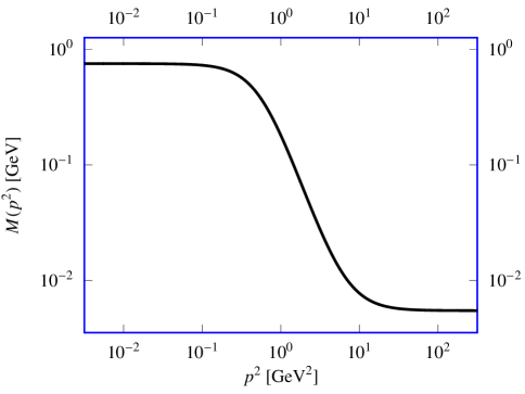
(a)

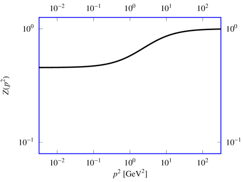
(b)

Figure 1: Mass function $M(\mbox{\boldmath{$p$}}^{2})$ (a) and wave-function renormalization function $Z(\mbox{\boldmath{$p$}}^{2})$ (b) of the exact propagator of the (light) u- and d-quarks obtained by numerical solution of the quark Dyson–Schwinger equation in the “renormalization-group-improved rainbow–ladder truncation” model of Ref.[4] as represented by the simple interpolation of Eqs. (5) and (4).

4 Pseudoscalar fermion–antifermion bound states

Now follow the path, paved in Refs.[25, 26, 27, 28, 29, 30, 31, 32], of the transformation of bound-state equations for Salpeter amplitudes $\Phi(\mbox{\boldmath{$p$}})$ to matrix eigenvalue problems fixing their radial components.

Consider, as the perhaps simplest example, fermion–antifermion bound states of spin $J,$ parity $P=(-1)^{J+1}$ and charge-conjugation quantum number $C=(-1)^{J}.$ In spectroscopic notation such states are labeled by ${}^{1}J_{J}.$ Because of the constraints $\Lambda_{1}^{\pm}(\mbox{\boldmath{$p$}}_{1})\,\Phi(\mbox{\boldmath{$p$}})\,\Lambda_{2}^{\pm}(\mbox{\boldmath{$p$}}_{2})=0$ the general expansion of the Salpeter amplitude $\Phi(\mbox{\boldmath{$p$}})$ over a complete set of Dirac matrices involves not the full 16 but only eight independent components. For our ${}^{1}J_{J}$ states only two of the latter, $\Phi_{1}(\mbox{\boldmath{$p$}})$ and $\Phi_{2}(\mbox{\boldmath{$p$}}),$ are relevant. With our notation for one-particle energy $E(\mbox{\boldmath{$p$}})$ and (generalized) Dirac Hamiltonian $H(\mbox{\boldmath{$p$}})$ introduced in Sec. 2 the corresponding Salpeter amplitude $\Phi(\mbox{\boldmath{$p$}})$ reads in the center-of-momentum frame of the particle–antiparticle system

$$\Phi(\mbox{\boldmath{$p$}})=\left[\Phi_{1}(\mbox{\boldmath{$p$}})\,\frac{H(\mbox{\boldmath{$p$}})}{E(\mbox{\boldmath{$p$}})}+\Phi_{2}(\mbox{\boldmath{$p$}})\right]\gamma_{5}\ .$$

Without loss of generality but for definiteness, focus to exactly the same physical system as studied in Refs.[29, 30, 31, 32]. Aiming at the description of mesons with the quantum numbers of the pion discuss quark–antiquark bound states of spin $J=0,$ that is, pseudoscalar states of spin-parity-charge conjugation assignment $J^{PC}=0^{-+}.$ Assume the kernel $\hat{K}(\mbox{\boldmath{$p$}},\mbox{\boldmath{$q$}})$ to be of convolution type with Dirac structure that of time-component Lorentz-vector interactions: $\hat{K}(\mbox{\boldmath{$p$}},\mbox{\boldmath{$q$}})=\hat{K}(\mbox{\boldmath{$p$}}-\mbox{\boldmath{$q$}})=V(\mbox{\boldmath{$p$}}-\mbox{\boldmath{$q$}})\,\gamma^{0}\otimes\gamma^{0}$ with $V(\mbox{\boldmath{$p$}}-\mbox{\boldmath{$q$}})$ any Lorentz-scalar potential function.

Upon factorizing off all dependence of the Salpeter amplitude $\Phi(\mbox{\boldmath{$p$}})$ on angular variables the exact-propagator instantaneous Bethe–Salpeter equation (3) may be reduced [25, 27] to a set of coupled equations for the radial factors of all the independent Salpeter components. For bound states composed of particle and corresponding antiparticle we clearly have, with $p\equiv|\mbox{\boldmath{$p$}}|,$ $Z_{1}(\mbox{\boldmath{$p$}}^{2})=Z_{2}(\mbox{\boldmath{$p$}}^{2})\equiv Z(p^{2})$ and $M_{1}(\mbox{\boldmath{$p$}}^{2})=M_{2}(\mbox{\boldmath{$p$}}^{2})\equiv M(p^{2}),$ which will also enter in $E_{1}(\mbox{\boldmath{$p$}})=E_{2}(\mbox{\boldmath{$p$}})=E(p)\equiv\sqrt{p^{2}+M^{2}(p^{2})}.$ The set of coupled equations governing the radial functions $\Phi_{1}(p)$ and $\Phi_{2}(p)$ in our independent Salpeter components $\Phi_{1}(\mbox{\boldmath{$p$}})$ and $\Phi_{2}(\mbox{\boldmath{$p$}})$ of ${}^{1}{\rm S}_{0}$ states, respectively, can be simply derived by, for instance, “dressing” Eq. (1) of Ref.[29] or Eq. (1) of Ref.[31] by insertion of the appropriate factors $Z(p^{2})$ in all interaction terms and by replacement of all constant constituent masses $m$ by the relevant mass functions $M(p^{2})$:

$$2\,E(p)\,\Phi_{2}(p)+Z^{2}(p^{2})\int\limits_{0}^{\infty}\frac{{\rm d}q\,q^{2}}{(2\pi)^{2}}\,V_{0}(p,q)\,\Phi_{2}(q)=M_{\rm B}\,\Phi_{1}(p)\ ,$$

$$2\,E(p)\,\Phi_{1}(p)$$ (6)

$$+\,Z^{2}(p^{2})\int\limits_{0}^{\infty}\frac{{\rm d}q\,q^{2}}{(2\pi)^{2}}\left[\frac{M(p^{2})}{E(p)}\,V_{0}(p,q)\,\frac{M(q^{2})}{E(q)}+\frac{p}{E(p)}\,V_{1}(p,q)\,\frac{q}{E(q)}\right]\Phi_{1}(q)=M_{\rm B}\,\Phi_{2}(p)\ .$$

The configuration- and momentum-space representations of any radial function are related by Fourier–Bessel transformations which involve spherical Bessel functions of the first kind $j_{n}(z)$ ($n=0,\pm 1,\pm 2,\dots$)[37]; as a kind of reminiscence of these, the interaction $V(\mbox{\boldmath{$p$}}-\mbox{\boldmath{$q$}})$ in the kernel $\hat{K}(\mbox{\boldmath{$p$}}-\mbox{\boldmath{$q$}})$ enters here in form of some static potential $V(r)$ in configuration space:

$$V_{L}(p,q)\equiv 8\pi\int\limits_{0}^{\infty}{\rm d}r\,r^{2}\,j_{L}(p\,r)\,j_{L}(q\,r)\,V(r)\ ,\quad L=0,1,2,\dots\ .$$

The particular structure of the set of equations (6) allows to find its solutions[29, 30, 31, 32] by inserting one of these relations into the other and obtaining an eigenvalue equation for $M_{\rm B}^{2}$:

$$M_{\rm B}^{2}\,\Phi_{2}(p) = 4\,E^{2}(p)\,\Phi_{2}(p)+2\,Z^{2}(p^{2})\,E(p)\int\limits_{0}^{\infty}\frac{{\rm d}q\,q^{2}}{(2\pi)^{2}}\,V_{0}(p,q)\,\Phi_{2}(q)$$ (7)

$$+ 2\,\frac{Z^{2}(p^{2})}{E(p)}\int\limits_{0}^{\infty}\frac{{\rm d}q\,q^{2}}{(2\pi)^{2}}\left[M(p^{2})\,M(q^{2})\,V_{0}(p,q)+p\,q\,V_{1}(p,q)\right]\Phi_{2}(q)$$

$$+ Z^{2}(p^{2})\int\limits_{0}^{\infty}\frac{{\rm d}q\,q^{2}}{(2\pi)^{2}}\left[\frac{M(p^{2})}{E(p)}\,V_{0}(p,q)\,\frac{M(q^{2})}{E(q)}+\frac{p}{E(p)}\,V_{1}(p,q)\,\frac{q}{E(q)}\right]$$

$$\times Z^{2}(q^{2})\int\limits_{0}^{\infty}\frac{{\rm d}k\,k^{2}}{(2\pi)^{2}}\,V_{0}(q,k)\,\Phi_{2}(k)\ .$$

By expansion over the basis for radial functions summarized in Appendix A we convert this integral equation to an equivalent matrix eigenvalue problem which can be diagonalized by standard means. As noted in Sec. 2, Salpeter’s equation corresponds to the free-propagator approximation $Z(p^{2})\cong 1$ and $M(p^{2})\cong m.$ Thus the studies reported in Refs.[29, 30, 31, 32] could get the matrix, for a large class of interactions, in algebraic form. Due to the presence of the true quark propagator functions $Z(p^{2})$ and $M(p^{2}),$ in general this is no longer possible here. Upon construction of one Salpeter component, $\Phi_{2}(p),$ as solution of Eq. (7), its companion, $\Phi_{1}(p),$ follows, for $M_{\rm B}\neq 0,$ immediately from the first of the two coupled equations (6). For vanishing bound-state mass, $M_{\rm B}=0,$ Eqs. (6) decouple and are thus solved independently.

5 Linear confinement: results and discussion

Let us eventually apply the formalism developed in Secs. 2 through 4 to a confining (static) potential of linear shape, $V(r)=\lambda\,r,$ with slope $\lambda=0.2\;\mbox{GeV}^{2}.$ For confining interactions a time-component Lorentz-vector structure of the kernel appears to be free of all the stability problems encountered by solutions found for a kernel of Lorentz-scalar structure[38, 39, 27].

Our first goal is to analyze the effect of the dynamical generation of quark masses on the solutions of the instantaneous Bethe–Salpeter equation (3) with exact propagators. To this end, Fig. 2 compares, for the three lowest positive-norm $J^{PC}=0^{-+}$ bound states, the mass eigenvalues $M_{\rm B}$ of Eq. (3) for exact light-quark propagators with $m_{0}=0$ (corresponding to the chiral limit of QCD) with those of a Salpeter equation for massless constituents [29, 30].

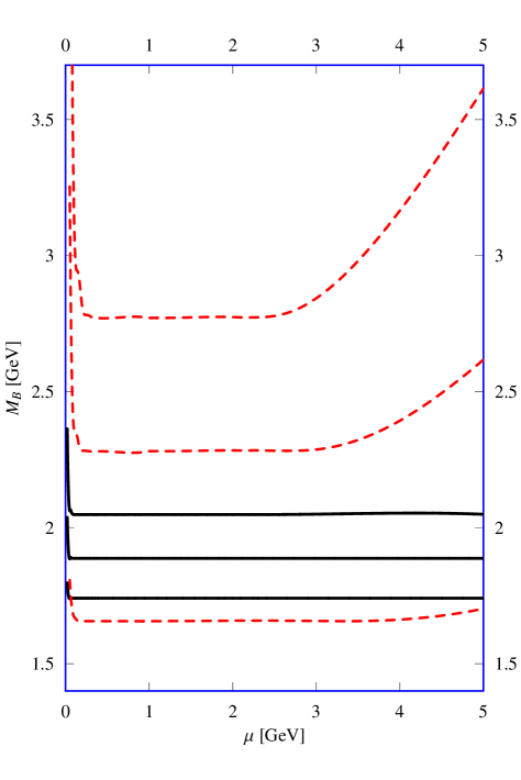
Figure 2: Bound-state masses $M_{\rm B}$ (as functions of our variational parameter $\mu$) of the three lowest-lying (positive-norm) $J^{PC}=0^{-+}$ eigenstates of our exact-propagator instantaneous Bethe–Salpeter equation (3) for the propagator parametrization (5) but $m_{0}=0$ (full lines) and of the Salpeter equation for massless constituents (dashed lines), for a time-component Lorentz-vector kernel representing some linear potential $V(r)=\lambda\,r$ of slope $\lambda=0.2\;\mbox{GeV}^{2}.$ These results arise from diagonalization, for given values of $\mu,$ of $50\times 50$ matrices equivalent to our exact-propagator equation but, mimicking Ref.[29], only $15\times 15$ matrices equivalent to Salpeter’s equation and in both cases 50 terms in all intermediate-step series expansions.

The chosen bases for the Hilbert space $L_{2}(R^{+})$ of all with the weight function $w(r)=r^{2}$ square-integrable (“radial”) functions on the positive real line $R^{+}$ introduce one additional degree of freedom, by allowing the basis states to depend on a variational parameter $\mu>0.$ As a basis, these vectors constitute a complete orthonormal system for any particular value of $\mu.$ Therefore, as long as relying exclusively on expansions over the full set of basis vectors our results may be expected to be independent of $\mu.$ Necessary truncations of expansions to a finite number of basis vectors will induce a certain amount of $\mu$-dependence of the results. However, a reasonable technique involving expansions should exhibit stability with respect to the increase of the number of basis vectors. If taking into account a large enough number of basis vectors, by reducing the dependence on $\mu$ some “region of stability” should emerge.

With respect to the mass $M_{\rm B}$ of a given bound state, such a region of stability manifests itself in form of a plateau where the numerical value predicted for $M_{\rm B}$ is constant over some nonvanishing range of $\mu.$ Beyond doubt, the formation of these plateaus is obvious in Fig. 2. Such extrema of $M_{\rm B}$ disclose the bound states. Compared with the free-propagator results, the ground state of Eq. (3) is higher but its radial excitations are lower, to the effect that all level spacings are significantly smaller if using exact propagators. In general, it is, of course, not possible to compensate for these shifts by some change of the parameter values entering in the interaction kernel. For instance, a reduction of the slope $\lambda$ of the linear potential by a factor 2 to $\lambda\cong 0.1\;\mbox{GeV}^{2}$ lowers the ground-state energy eigenvalue of Eq. (3) to the level of its Salpeter-equation counterpart but simultaneously diminishes the level spacings further.

Table 1 lists the masses $M_{\rm B}$ of the three lowest-lying (positive-norm) $J^{PC}=0^{-+}$ bound states calculated from the exact-propagator instantaneous Bethe–Salpeter equation (3) for the full ($m_{0}\neq 0$) parametrization (5) and (4) of the exact light-quark propagators. Because of the relative smallness of the (explicitly chiral-symmetry breaking) current mass $m_{0}$ these eigenvalues are, of course, less than some 0.5% larger than the corresponding “chiral-limit” values forming the stability plateaus discernible in Fig. 2. These mass values are confronted in Table 1 with the corresponding mass eigenvalues $M_{\rm B}$ of the Salpeter equation, computed by assuming, for the constituent mass $m$ of the light u- and d-quarks entering their effective propagators, the typical value of $m=0.336\;{\rm GeV}$ frequently adopted by nonrelativistic and relativistic constituent quark models to describe hadrons as bound states of quarks[40, 41]. Raising in the Salpeter equation the constituent quark mass $m$ from $m=0$ to the canonical value $m=0.336\;{\rm GeV}$ shifts the masses $M_{\rm B}$ of the three lowest states by more than $0.1\;{\rm GeV}$ towards larger values. The net result of this is a further increase of the discrepancy between the level spacings predicted by the exact-propagator equation (3) and the ones arising from the free-propagator Salpeter equation with some kind of appropriate or reasonable effective mass of the constituent quarks. Therefore, we are forced to conclude that any neglect of the proper behaviour of the momentum-dependent quark mass, $M(p^{2}),$ by approximating it by a constant constituent mass $m$ is, at least for the light u- and d-quarks, rather questionable.

Table 1: Bound-state masses $M_{\rm B}$ (in units of GeV) for the three lowest-lying positive-norm $J^{PC}=0^{-+}$ eigenstates (denoted by $1^{1}{\rm S}_{0},$ $2^{1}{\rm S}_{0},$ $3^{1}{\rm S}_{0},$ in usual spectroscopic notation) of our exact-propagator instantaneous Bethe–Salpeter equation (3) with light-quark propagators parametrized by Eqs. (5), (4) and of the free-propagator Salpeter equation with light-quark constituent mass $m=0.336\;{\rm GeV},$ for time-component Lorentz-vector kernels representing a linear potential $V(r)=\lambda\,r$ of slope $\lambda=0.2\;\mbox{GeV}^{2},$ obtained by converting both equations to $50\times 50$ matrices and taking into account 50 terms in intermediate-step series expansions.

State	Exact-propagator bound-state equation	(Free-propagator) Salpeter equation
$1^{1}{\rm S}_{0}$	1.750	1.813
$2^{1}{\rm S}_{0}$	1.895	2.410
$3^{1}{\rm S}_{0}$	2.056	2.889

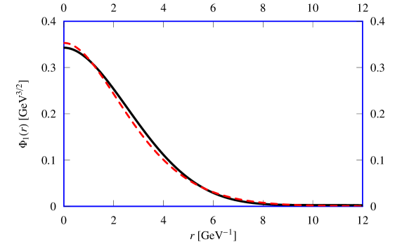
(a)

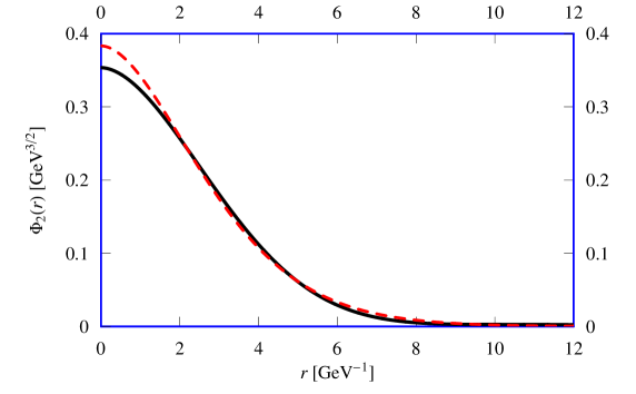
(b)

Figure 3: Configuration-space radial Salpeter component functions $\Phi_{1}(r)$ (a) and $\Phi_{2}(r)$ (b) for the lowest positive-norm $J^{PC}=0^{-+}$ bound state of the exact-propagator instantaneous Bethe–Salpeter equation (3) with the quark propagator parametrization (5) (full lines) and of the Salpeter equation with a light-quark constituent mass $m=0.336\;{\rm GeV}$ (dashed lines) for time-component Lorentz-vector kernels with linear potential $V(r)=\lambda\,r,$ $\lambda=0.2\;\mbox{GeV}^{2}.$

Figure 3 illustrates for the $J^{PC}=0^{-+}$ ground state ($1^{1}{\rm S}_{0}$ state) of the exact-propagator instantaneous Bethe–Salpeter equation (3) with quark-propagator parametrization (5) the configuration-space behaviour of the radial Salpeter component functions $\Phi_{1}(r)$ and $\Phi_{2}(r).$ The norm $\|\Phi\|$ of the Salpeter amplitude $\Phi(\mbox{\boldmath{$p$}})$ for $J^{PC}=0^{-+}$ bound states reads[25, 27, 29]

$$\|\Phi\|^{2}=4\int\frac{{\rm d}^{3}p}{(2\pi)^{3}}\,[\Phi_{1}^{\ast}(\mbox{\boldmath{$p$}})\,\Phi_{2}(\mbox{\boldmath{$p$}})+\Phi_{2}^{\ast}(\mbox{\boldmath{$p$}})\,\Phi_{1}(\mbox{\boldmath{$p$}})]\ ;$$

this translates for the radial parts $\Phi_{1}(p),$ $\Phi_{2}(p)$ of the Salpeter components $\Phi_{1}(\mbox{\boldmath{$p$}}),$ $\Phi_{2}(\mbox{\boldmath{$p$}})$ to

$$\|\Phi\|^{2}=\frac{4}{(2\pi)^{3}}\int\limits_{0}^{\infty}{\rm d}p\,p^{2}\,[\Phi_{1}^{\ast}(p)\,\Phi_{2}(p)+\Phi_{2}^{\ast}(p)\,\Phi_{1}(p)]\ .$$

For the plots depicted in Fig. 3, the normalization has been chosen such that $\Phi_{2}(r)$ satisfies

$$\int\limits_{0}^{\infty}{\rm d}r\,r^{2}\,|\Phi_{2}(r)|^{2}=\int\limits_{0}^{\infty}{\rm d}p\,p^{2}\,|\Phi_{2}(p)|^{2}=1\ ;$$

the first of Eqs. (6) fixes, after a Fourier–Bessel transformation, the normalization of $\Phi_{1}(r).$ A normalization factor common to $\Phi_{1}(p)$ and $\Phi_{2}(p)$ will then give any desired value to $\|\Phi\|.$

A closer inspection of the radial Salpeter components $\Phi_{1}(r)$ and $\Phi_{2}(r)$ reveals a striking similarity to their counterparts found as solutions of the Salpeter equation for a constituent quark mass of $m=0.336\;{\rm GeV}.$ Exact- and free-propagator Salpeter components $\Phi_{1}(r)$ and $\Phi_{2}(r)$ show some notable difference only for $r<5\;{\rm GeV}^{-1}$ for $\Phi_{1}(r)$ and for $r<2\;{\rm GeV}^{-1}$ for $\Phi_{2}(r).$ They are hardly distinguishable from each other for $r>5\;{\rm GeV}^{-1}$ for both $\Phi_{1}(r)$ and $\Phi_{2}(r).$ Thus we feel entitled to expect similar predictions for quantities such as decay rates.

6 Summary, conclusions, and outlook

The reduction of the Bethe–Salpeter formalism to the Salpeter equation requires to assume for all bound-state constituents not only an instantaneous interaction but also free-particle propagation. Realizing this fact, a bound-state equation that retains the exact propagators of the bound-state constituents and generalizes Salpeter’s equation has been formulated by consequent application of the instantaneous approximation to all exact propagators too[3]. Of course, this may be extended to Bethe–Salpeter equations for bound states composed of particles that are not, or not all, identical to spin-$\frac{1}{2}$ fermions as well as to three-dimensional reductions[42, 43, 44, 45] of the Bethe–Salpeter equation[1] different from Salpeter’s equation[2].

The present investigation addressed the question of how realistic descriptions of mesons as quark–antiquark bound states within a general instantaneous Bethe–Salpeter formalism will be modified by such reinstallment of the exact quark propagators, extracted from QCD by analytic continuation from Euclidean to Minkowski space. Interestingly, for the example of a specific interaction used already in earlier studies [27, 28, 29, 30, 31, 32], we find a drastic shrinking of the level spacings of the bound states while their amplitudes remain practically unchanged.

Appendix A The generalized Laguerre basis for radial functions

The Hilbert space $L_{2}(R^{3})$ of all square-integrable functions on the 3-dimensional Euclidean space $R^{3}$ can be spanned by basis functions each of which is the product of a function of the radial variable and of an angular term, the latter being represented by a spherical harmonic ${\cal Y}_{\ell m}(\Omega)$ for the angular momentum $\ell=0,1,2,\dots$ and its projection $m=-\ell,-\ell+1,\dots,+\ell$ which all depend on the solid angle $\Omega\equiv(\theta,\phi)$ and satisfy the orthonormalization condition

$$\int{\rm d}\Omega\,{\cal Y}^{\ast}_{\ell m}(\Omega)\,{\cal Y}_{\ell^{\prime}m^{\prime}}(\Omega)=\delta_{\ell\ell^{\prime}}\,\delta_{mm^{\prime}}\ .$$

For each value of $\ell$ the radial functions constitute a basis for the Hilbert space $L_{2}(R^{+})$ of all with the weight function $w(r)=r^{2}$ square-integrable functions on the positive real line $R^{+}.$ The basis functions of $L_{2}(R^{3})$ in configuration and momentum space are related by Fourier transformation. Thus, the configuration-space representation $\phi_{i}^{(\ell)}(r)$ and momentum-space representation $\phi_{i}^{(\ell)}(p)$ of the radial factors are related by the Fourier–Bessel transformation

$$\phi_{i}^{(\ell)}(r) = {\rm i}^{\ell}\,\sqrt{\frac{2}{\pi}}\int\limits_{0}^{\infty}{\rm d}p\,p^{2}\,j_{\ell}(p\,r)\,\phi_{i}^{(\ell)}(p)\ ,\quad i=0,1,2,\dots\ ,\quad\ell=0,1,2,\dots\ ,$$

$$\phi_{i}^{(\ell)}(p) = (-{\rm i})^{\ell}\,\sqrt{\frac{2}{\pi}}\int\limits_{0}^{\infty}{\rm d}r\,r^{2}\,j_{\ell}(p\,r)\,\phi_{i}^{(\ell)}(r)\ ,\quad i=0,1,2,\dots\ ,\quad\ell=0,1,2,\dots\ .$$

The spherical Bessel functions of the first kind, $j_{n}(z)$ ($n=0,\pm 1,\pm 2,\dots$)[37], are remnants of the angular integration. This may be easily deduced with the help of the expansion of the plane waves over spherical harmonics ${\cal Y}_{\ell m}$ in configuration $(\Omega_{r})$ and momentum $(\Omega_{p})$ space

$$\exp({\rm i}\,\mbox{\boldmath{$p$}}\cdot\mbox{\boldmath{$x$}})=4\pi\,\sum_{\ell=0}^{\infty}\,\sum_{m=-\ell}^{+\ell}\,{\rm i}^{\ell}\,j_{\ell}(p\,r)\,{\cal Y}^{\ast}_{\ell m}(\Omega_{p})\,{\cal Y}_{\ell m}(\Omega_{r})\ .$$

In terms of orthogonal polynomials of generalized-Laguerre type (for parameter $\gamma$)[37],

$$L_{i}^{(\gamma)}(x)=\sum_{t=0}^{i}\,(-1)^{t}\left(\begin{array}[]{c}i+\gamma\\ i-t\end{array}\right)\frac{x^{t}}{t!}\ ,\quad i=0,1,2,\dots\ ,$$

which, by construction, are orthonormalized [with weight $w(x)=x^{\gamma}\exp(-x)]$ according to

$$\int\limits_{0}^{\infty}{\rm d}x\,x^{\gamma}\exp(-x)\,L_{i}^{(\gamma)}(x)\,L_{j}^{(\gamma)}(x)=\frac{\Gamma(\gamma+i+1)}{i!}\,\delta_{ij}\ ,\quad i,j=0,1,2,\dots\ ,$$

our favourite choice of these radial bases is defined in configuration-space representation by

$$\phi_{i}^{(\ell)}(r)=\sqrt{\frac{(2\,\mu)^{2\,\ell+3}\,i!}{\Gamma(2\,\ell+i+3)}}\,r^{\ell}\exp(-\mu\,r)\,L_{i}^{(2\,\ell+2)}(2\,\mu\,r)\ ,\quad i=0,1,2,\dots\ .$$

These basis functions involve one positive real variational parameter, with the dimension of mass, $\mu.$ The requirement of their normalizability imposes the constraint $\mu>0.$ Then these configuration-space radial basis functions, $\phi_{i}^{(\ell)}(r),$ satisfy the orthonormalization condition

$$\int\limits_{0}^{\infty}{\rm d}r\,r^{2}\,\phi_{i}^{(\ell)}(r)\,\phi_{j}^{(\ell)}(r)=\delta_{ij}\ ,\quad i,j=0,1,2,\dots\ .$$

Note that the configuration-space representation of our basis functions is chosen to be real.

The corresponding momentum-space representation $\phi_{i}^{(\ell)}(p)$ of our basis functions reads

$$\phi_{i}^{(\ell)}(p) = \sqrt{\frac{(2\,\mu)^{2\,\ell+3}\,i!}{\Gamma(2\,\ell+i+3)}}\,\frac{(-{\rm i})^{\ell}\,p^{\ell}}{2^{\ell+1/2}\,\Gamma\left(\ell+\frac{3}{2}\right)}\,$$

$$\times \sum_{t=0}^{i}\,\frac{(-1)^{t}}{t!}\left(\begin{array}[]{c}i+2\,\ell+2\\ i-t\end{array}\right)\frac{\Gamma(2\,\ell+t+3)\,(2\,\mu)^{t}}{(p^{2}+\mu^{2})^{(2\,\ell+t+3)/2}}$$

$$\times F\left(\frac{2\,\ell+t+3}{2},-\frac{1+t}{2};\ell+\frac{3}{2};\frac{p^{2}}{p^{2}+\mu^{2}}\right),\quad i=0,1,2,\dots\ ,$$

with the hypergeometric series $F(u,v;w;z)$ given in terms of the gamma function $\Gamma$ by[37]

$$F(u,v;w;z)=\frac{\Gamma(w)}{\Gamma(u)\,\Gamma(v)}\,\sum_{n=0}^{\infty}\,\frac{\Gamma(u+n)\,\Gamma(v+n)}{\Gamma(w+n)}\,\frac{z^{n}}{n!}\ .$$

The momentum-space radial basis functions $\phi_{i}^{(\ell)}(p)$ fulfill the orthonormalization condition

$$\int\limits_{0}^{\infty}{\rm d}p\,p^{2}\,\phi_{i}^{\ast(\ell)}(p)\,\phi_{j}^{(\ell)}(p)=\delta_{ij}\ ,\quad i,j=0,1,2,\dots\ .$$

In momentum space, our basis functions are real for $\ell=0,$ as well as for all even values of $\ell$:

$$\phi_{i}^{\ast(\ell)}(p)=\phi_{i}^{(\ell)}(p)\quad\mbox{for\ }\ell=0,2,4,\dots\ ,\quad\forall\ i=0,1,2,\dots\ .$$

The virtue of our bases is their analytic availability in configuration and momentum space.

Mainly for computational convenience, the present investigation makes use of the radial basis functions for two values $\ell=0$ and $\ell=1$ of the angular momentum. Having to deal, in momentum-space representation, with the cumbersome hypergeometric series $F(u,v;w;z)$ may be avoided by employing simplified expressions equivalent to the above definition[46]:

$$\phi_{i}^{(0)}(p) = \sqrt{\frac{i!}{\mu\,\pi\,\Gamma(i+3)}}\,\frac{4}{p}\,\sum_{t=0}^{i}\,(-2)^{t}\,(t+1)\left(\begin{array}[]{c}i+2\\ i-t\end{array}\right)\left(1+\frac{p^{2}}{\mu^{2}}\right)^{-(t+2)/2}$$

$$\times \sin\left((t+2)\arctan\frac{p}{\mu}\right)$$

$$= \frac{{\rm Im}\{(p+{\rm i}\,\mu)^{2\,i+3}\,[p-{\rm i}\,(3+2\,i)\,\mu]\}}{\sqrt{\mu\,\pi\,(i+1)\,(i+2)}\,p\,(p^{2}+\mu^{2})^{2+i}}\ ,$$

$$\phi_{i}^{(1)}(p) = -{\rm i}\,\sqrt{\frac{\mu^{5}}{\pi\,(i+1)\,(i+2)\,(i+3)\,(i+4)}}\,\frac{8}{p^{2}}\,\sum_{t=0}^{i}\,\frac{(-2)^{t}}{t!}\left(\begin{array}[]{c}i+4\\ i-t\end{array}\right)\frac{(t+3)!\,\mu^{t}}{(p^{2}+\mu^{2})^{(t+3)/2}}$$

$$\times \left[\frac{\sqrt{p^{2}+\mu^{2}}}{t+2}\sin\left((t+2)\arctan\frac{p}{\mu}\right)-\frac{\mu}{t+3}\sin\left((t+3)\arctan\frac{p}{\mu}\right)\right]$$

$$= \frac{{\rm i}}{2\,\sqrt{\mu^{3}\,\pi\,(i+1)\,(i+2)\,(i+3)\,(i+4)}\,p^{2}\,(p^{2}+\mu^{2})^{3}}$$

$$\times {\rm Im}\left\{\frac{(p-{\rm i}\,\mu)^{i+5}}{(p+{\rm i}\,\mu)^{i}}\,[3\,p^{3}+3\,{\rm i}\,(5+2\,i)\,p^{2}\,\mu-(5+2\,i)^{2}\,p\,\mu^{2}-{\rm i}\,(5+2\,i)\,\mu^{3}]\right\}.$$

References

- [1] E. E. Salpeter and H. A. Bethe, Phys. Rev. 84 (1951) 1232.
- [2] E. E. Salpeter, Phys. Rev. 87 (1952) 328.
- [3] W. Lucha and F. F. Schöberl, J. Phys. G: Nucl. Part. Phys. 31 (2005) 1133, hep-th/0507281.
- [4] P. Maris and C. D. Roberts, Phys. Rev. C 56 (1997) 3369, nucl-th/9708029.
- [5] P. Maris and C. D. Roberts, in: Proc. of the IVth Int. Workshop on Progress in Heavy Quark Physics, edited by M. Beyer, T. Mannel, and H. Schröder (University of Rostock, Rostock, 1998), p. 159, nucl-th/9710062.
- [6] C. D. Roberts, in: Proc. of the 11th Physics Summer School on Frontiers in Nuclear Physics: From Quark–Gluon Plasma to Supernova, edited by S. Kuyucak (World Scientific, Singapore, 1999), p. 212, nucl-th/9807026.
- [7] M. A. Ivanov, Yu. L. Kalinovsky, and C. D. Roberts, Phys. Rev. D 60 (1999) 034018, nucl-th/9812063.
- [8] P. Maris and P. C. Tandy, Phys. Rev. C 60 (1999) 055214, nucl-th/9905056.
- [9] P. Maris, Nucl. Phys. A 663 (2000) 621, nucl-th/9908044.
- [10] C. D. Roberts and S. M. Schmidt, Prog. Part. Nucl. Phys. 45 (2000) S1, nucl-th/0005064.
- [11] C. D. Roberts, nucl-th/0007054.
- [12] R. Alkofer and L. von Smekal, Phys. Rep. 353 (2001) 281, hep-ph/0007355.
- [13] P. Maris, in: Proc. of the Int. Conf. on Quark Confinement and the Hadron Spectrum IV, edited by W. Lucha and K. Maung Maung (World Scientific, New Jersey/London/Singapore/Hong Kong, 2002), p. 163, nucl-th/0009064.
- [14] P. Maris and P. C. Tandy, nucl-th/0109035.
- [15] P. Maris, A. Raya, C. D. Roberts, and S. M. Schmidt, Eur. Phys. J. A 18 (2003) 231, nucl-th/0208071.
- [16] M. S. Bhagwat, M. A. Pichowsky, and P. C. Tandy, Phys. Rev. D 67 (2003) 054019, hep-ph/0212276.
- [17] P. C. Tandy, Prog. Part. Nucl. Phys. 50 (2003) 305, nucl-th/0301040.
- [18] P. Maris and C. D. Roberts, Int. J. Mod. Phys. E 12 (2003) 297, nucl-th/0301049.
- [19] M. S. Bhagwat, M. A. Pichowsky, C. D. Roberts, and P. C. Tandy, Phys. Rev. C 68 (2003) 015203, nucl-th/0304003.
- [20] C. D. Roberts, Lect. Notes Phys. 647 (2004) 149, nucl-th/0304050.
- [21] A. Krassnigg and C. D. Roberts, Fizika B 13 (2004) 143, nucl-th/0308039.
- [22] A. Krassnigg and C. D. Roberts, Nucl. Phys. A 737 (2004) 7, nucl-th/0309025.
- [23] R. Alkofer, W. Detmold, C. S. Fischer, and P. Maris, Phys. Rev. D 70 (2004) 014014, hep-ph/0309077.
- [24] A. Krassnigg and P. Maris, J. Phys. Conf. Ser. 9 (2005) 153, nucl-th/0412058.
- [25] J.-F. Lagaë, Phys. Rev. D 45 (1992) 305.
- [26] J.-F. Lagaë, Phys. Rev. D 45 (1992) 317.
- [27] M. G. Olsson, S. Veseli, and K. Williams, Phys. Rev. D 52 (1995) 5141, hep-ph/9503477.
- [28] M. G. Olsson, S. Veseli, and K. Williams, Phys. Rev. D 53 (1996) 504, hep-ph/9504221.
- [29] W. Lucha, K. Maung Maung, and F. F. Schöberl, Phys. Rev. D 63 (2001) 056002, hep-ph/0009185.
- [30] W. Lucha, K. Maung Maung, and F. F. Schöberl, in: Proc. of the Int. Conf. on Quark Confinement and the Hadron Spectrum IV, edited by W. Lucha and K. Maung Maung (World Scientific, New Jersey/London/Singapore/Hong Kong, 2002), p. 340, hep-ph/0010078.
- [31] W. Lucha, K. Maung Maung, and F. F. Schöberl, Phys. Rev. D 64 (2001) 036007, hep-ph/0011235.
- [32] W. Lucha and F. F. Schöberl, Int. J. Mod. Phys. A 17 (2002) 2233, hep-ph/0109165.
- [33] P. Maris, Phys. Rev. D 50 (1994) 4189.
- [34] R. Alkofer, W. Detmold, C. S. Fischer, and P. Maris, Nucl. Phys. Proc. Suppl. 141 (2005) 122, hep-ph/0309078.
- [35] C. D. Roberts (private communication).
- [36] P. O. Bowman, U. M. Heller, D. B. Leinweber, M. B. Parappilly, A. G. Williams, and J.-B. Zhang, Phys. Rev. D 71 (2005) 054507, hep-lat/0501019.
- [37] Handbook of Mathematical Functions, edited by M. Abramowitz and I. A. Stegun (Dover, New York, 1964).
- [38] J. Parramore and J. Piekarewicz, Nucl. Phys. A 585 (1995) 705, nucl-th/9402019.
- [39] J. Parramore, H.-C. Jean, and J. Piekarewicz, Phys. Rev. C 53 (1996) 2449, nucl-th/9510024.
- [40] W. Lucha, F. F. Schöberl, and D. Gromes, Phys. Rep. 200 (1991) 127.
- [41] W. Lucha and F. F. Schöberl, Int. J. Mod. Phys. A 7 (1992) 6431.
- [42] T. Babutsidze, T. Kopaleishvili, and A. Rusetsky, Phys. Lett. B 426 (1998) 139, hep-ph/9710278.
- [43] T. Babutsidze, T. Kopaleishvili, and A. Rusetsky, Phys. Rev. C 59 (1999) 976, hep-ph/9807485.
- [44] T. Kopaleishvili, Phys. Part. Nucl. 32 (2001) 560, hep-ph/0101271.
- [45] T. Babutsidze, T. Kopaleishvili, and D. Kurashvili, Georgian Electronic Scientific J.: Phys. 1 (2004) 20, hep-ph/0308072.
- [46] W. Lucha and F. F. Schöberl, Phys. Rev. A 56 (1997) 139, hep-ph/9609322.