Abstract

We suggest a supersymmetric (SUSY) explanation of neutrino masses and mixing, where nonrenormalizable interactions in the hidden sector generate lepton number violating Majorana mass terms for both right-chiral sneutrinos and neutrinos. It is found necessary to start with a superpotential including an array of gauge singlet chiral superfields. This leads to nondiagonal $\Delta L=2$ mass terms and almost diagonal SUSY breaking $A$-terms. As a result, the observed pattern of bilarge mixing can be naturally explained by the simultaneous existence of the seesaw mechanism and radiatively induced masses. Allowed ranges of parameters in the gauge singlet sector are delineated, corresponding to each of the cases of normal hierarchy, inverted hierarchy and degenerate neutrinos.

PACS indices: 12.60.Jv, 14.60.Lm, 14.60.Pq, 14.60.St

1 Introduction

With the evidence in favor of neutrino masses and mixing at a convincing level now, attempts to seek the role of physics beyond the standard model in the neutrino sector are acquiring enhanced degrees of urgency. As it is, the lack of naturalness of the mass of the Higgs boson in the standard model is a strong pointer towards new physics around the TeV scale. Since tiny masses can be explained by appealing to energy scales much higher than the electroweak scale (for example in the seesaw mechanism), it is appropriate to link neutrino mass generation to new physics options at the TeV scale or above.

Supersymmetry (SUSY) is a frequently explored possibility for new TeV-scale physics. Its capability for solving the naturalness problem being an accepted fact, serious efforts are on at accelerators to see signals of SUSY, broken with an intra-supermultiplet mass splitting $\cal O$(TeV). Does SUSY play a role in providing the requisite new physics component in the masses and mixing pattern of neutrinos? This is the question that we would like to address. Often one has to go beyond the minimal SUSY standard model (MSSM) in order to find satisfactory mechanisms which can achieve this end. Though a fair amount of work has been done in this area [1], one is yet to have a satisfactory answer to the following central question related to the neutrino sector. Why is the mixing pattern of neutrinos, with two large and one small mixing angles, so drastically different from that in the quark sector, where the mixing between the three generations can be cryptically described by the progression - small, smaller, smallest?

In this paper we approach the above problem with the idea that the difference between the two mixing patterns arises from some aspects of the SUSY model which are specific to neutrinos and with no counterparts in the quark sector. For this, we make use of nonrenormalizable terms arising from high-scale physics. Such terms, coupling some hidden sector (gauge singlet) chiral superfields to the MSSM ones, are suppressed by the Planck mass $M_{P}$ or some power of it. If these terms violate lepton number , they can lead to Majorana masses for neutrinos. When, in addition, there are superfields containing right-chiral neutrinos, contributions to the neutrino mass matrix can come not only from the well-known seesaw mechanism but also radiatively via one-loop diagrams containing right chiral sneutrinos. Though both these contributions have been included in earlier works [2, 3, 4], a clear explanation of the different character of mixing for neutrinos vis-a-vis quarks has been lacking without the imposition of some additional restriction on the low-energy theory. The Froggatt-Nielsen mechanism [5] is an example of such additional theoretical inputs. The literature, of course, is rich with uses of various other symmetries [6], as well as of ‘anarchy’ in the neutrino mass matrix [7]. Drawing inspiration from all these approaches, we suggest an alternative justification of bilarge neutrino mixing by postulating an array of gauge singlet chiral superfields with flavor-dependent nonrenormalizable couplings to neutrinos. The specific superpotential that yields the desired results is formulated, and consistency with the observed suppression of flavour-changing neutral currents (FCNC) in the lepton sector is used as a constraint. One further has radiative contributions, pertaining only to the neutrino mass matrix. These are due to the fact that the right chiral sneutrinos may acquire gauge singlet $\Delta L=2$ mass terms. The scenario for neutrinos then immediately becomes quite distinct from that in the quark sector.

Using the standard seesaw as well as the above-mentioned radiative contributions, we have examined whether high-scale parameters, such as the vacuum expectation values (VEV) of scalar as well as of auxiliary components of the gauge singlet chiral superfields, crucial to this mechanism, are in otherwise acceptable ranges of values. For instance, the Higgsino mass ($\mu$) parameter needs to be around the weak scale for the desired implementation of the spontaneous breakdown of electroweak symmetry. Such analyses are carried out for the three alternative possibilitiess of the neutrino mass spectrum allowed by the neutrino oscillation data, namely, normal hierarchy, inverted hierarchy and degenerate neutrinos. The simultaneous importance of the radiative as well as the seesaw contributions enables us to acquire in all the three scenarios substantial regions (of different extent in each case) in the parameter space of our model that correspond to acceptable solutions.

In section 2 we describe the (by now well-known) structure of the neutrino mass matrix $M_{\nu}$ for bilarge mixing. The SUSY model is constructed and the elements of $M_{\nu}$ are consistently generated in section 3; we also show at the end of this section how FCNC processes, induced at one loop, are suppressed. The SUSY parameter space, answering to each of the specific scenarios of normal hierarchy, inverted hierarchy and degenerate neutrinos, is analyzed in section 4. We comment on some related possibilities in section 5. Section 6 contains our summary and conclusions.

2 Facts about neutrinos

There is experimental evidence now that neutrinos have tiny masses. We shall work within the scheme of three light active neutrinos, not including the possibility of an additional light sterile one suggested by the LSND data till results from the ongoing mini-Boone experiment settle the issue. We shall further assume CPT conservation. While there is an upper bound [8] of $\sim 1$ eV on the sum of neutrino mass eigenvlaues from cosmology, the lack of observation of neutrinoless double beta decay implies an upper bound of $\sim 0.3$ eV on the absolute value of the the 11-element of the neutrino mass matrix [9]. On the other hand, the accumulating data from solar, atmospheric, accelerator and reactor neutrino experiments persistently point [10] towards neutrino oscillations. These data identify favored regions of small but distinct mass-squared separation of the three different physical neutrino states. At the same time, they also indicate that the mixing between the second and the third families is near maximal, that between the first and the second is large, while the one between the first and the third families is restricted to a small angle. In perfect analogy with the Cabibbo-Kobayashi-Maskawa (CKM) matrix in the quark sector, the three-flavour neutrino mixing matrix can be parameterized as

$$U=\left(\begin{array}[]{ccc}c_{12}c_{13}&s_{12}c_{13}&s_{13}e^{-i\delta}\\ -s_{12}c_{23}-c_{12}s_{23}s_{13}e^{i\delta}&c_{12}c_{23}-s_{12}s_{23}s_{13}e^{i\delta}&s_{23}c_{13}\\ s_{12}s_{23}-c_{12}c_{23}s_{13}e^{i\delta}&-c_{12}s_{23}-s_{12}c_{23}s_{13}e^{i\delta}&c_{23}c_{13}\end{array}\right).$$ (4)

In Eq. (1) $c_{ij}=\cos\theta_{ij}$, $s_{ij}=\sin\theta_{ij}$, $i,j$ being family indices which run from 1 to 3 (Majorana phases have been neglected here). We work in the basis where the charged lepton mass matrix is diagonalized. While solar (reactor) neutrino (antineutrino) studies suggest that $\theta_{12}\simeq 32^{o}$ [11, 12], the atmospheric neutrino deficit needs $\theta_{23}$ to be $\sim 45^{o}$ [13] and data from reactors require that $\theta_{13}\leq 13^{o}$ [14]. Thus a pattern of bilarge mixing emerges.

The above pattern allows one to construct a candidate neutrino mass matrix in terms of the mass eigenvalues $m_{1},m_{2},m_{3}$. To start with, let us take $\theta_{23}=\frac{\pi}{4}$ and $\theta_{13}=0$ approximately, keeping $\theta_{12}$ free to be large. Then the corresponding transformation matrix can be written as

$$U_{\nu}=\left(\begin{array}[]{ccc}c&s&0\\ -\frac{s}{\sqrt{2}}&\frac{c}{\sqrt{2}}&\frac{1}{\sqrt{2}}\\ \frac{s}{\sqrt{2}}&-\frac{c}{\sqrt{2}}&\frac{1}{\sqrt{2}}\end{array}\right),$$ (8)

where $s=\sin\theta_{12}$ and $c=\cos\theta_{12}$. The neutrino Majorana mass matrix in the flavor basis can now be obtained by transforming the diagonal matrix with the above:

$$M_{\nu} = U_{\nu}\left(\begin{array}[]{ccc}m_{1}&&\\ &m_{2}&\\ &&m_{3}\end{array}\right)U^{T}_{\nu}$$ (12)

$$= \left(\begin{array}[]{ccc}m_{1}c^{2}+m_{2}s^{2}&\frac{cs}{\sqrt{2}}(-m_{1}+m_{2})&\frac{cs}{\sqrt{2}}(m_{1}-m_{2})\\ \frac{cs}{\sqrt{2}}(-m_{1}+m_{2})&\frac{1}{2}(m_{1}s^{2}+m_{2}c^{2}+m_{3})&\frac{1}{2}(-m_{1}s^{2}-m_{2}c^{2}+m_{3})\\ \frac{cs}{\sqrt{2}}(m_{1}-m_{2})&\frac{1}{2}(-m_{1}s^{2}-m_{2}c^{2}+m_{3})&\frac{1}{2}(m_{1}s^{2}+m_{2}c^{2}+m_{3})\end{array}\right).$$ (16)

Thus we see that the requirement of bilarge mixing commits one to a particular structure of the mass matrix where, of course, the relative magnitudes of the entries depend on the eigenvalues. For more precise information one has to take up the specific scenario of normal/inverted hierarchy or that of degenerate neutrinos. In our study, we attempt to link the diagonal and off-diagonal mass terms of $M_{\nu}$ to the parameters of the SUSY model at high scale and see what the different scenarios tell us about the model parameters themselves.

3 The SUSY model and neutrino masses

3.1 Required features of the model

The model that we adopt is motivated by a number of recent works [2, 3, 4]. In  [3], for example, a minimal extension of the MSSM, including a right-handed neutrino, is used. There the terms of the effective Lagrangian responsible for neutrino masses are

$${\cal L}_{eff}=\frac{1}{M_{P}}\left([X^{\dagger}NN]_{D}+\left[XLNH_{u}\right]_{F}\right)+{\rm h.c.},$$ (17)

where $M_{P}$ is Planck scale and coupling coefficients of order unity have been suppressed. In Eq. (4), the chiral field $X$ can acquire both SUSY violating and SUSY conserving VEVs [15]. The above terms can be responsible for seesaw masses of order ${\frac{{F^{2}_{X}}}{M_{P}^{3}}}$ for the neutrinos (recalling the need to have $F_{X}\sim\langle x\rangle^{2}\sim M_{P}\langle H_{u}\rangle$, to ensure the generation of other superparticle masses in the TeV range) . In addition, there can be radiative contributions to the mass matrix from $\Delta L=2$ sneutrino mass terms after SUSY breaking. These can arise with the help of a term $\frac{1}{M_{P}^{3}}[X^{\dagger}XX^{\dagger}NN]_{D}$, making contributions that can dominate over seesaw masses in certain regions of the parameter space.

We aim to explain the bilarge mixing pattern of neutrinos by extending such a model. As mentioned earlier, the basic philosophy is to envision some feature of neutrinos, which has no counterpart in the quark sector, as being responsible for the observed bilarge mixing. There are two features of this kind in such a model: (a) the right-chiral neutrino sector and (b) the corresponding right-chiral sneutrino sector, with provisions of $\Delta L=2$ terms in each. In our approach, each of these sectors is attributed with a $3\times 3$ mass matrix structure which plays a crucial role in the contribution to the radiative as well as seesaw mass terms. Moreover, we postulate an array of gauge singlet chiral superfields $X_{ij}$. Following these propositions, Eq.(4) is generalized to

$${\cal L}_{eff}=\frac{1}{M_{P}}\left([X_{ij}^{\dagger}N^{i}N^{j}]_{D}+\left[X_{ij}L^{i}N^{j}H_{u}\right]_{F}\right)+{\rm h.c.},$$ (18)

where there is a summation over flavor (i.e. generation) indices $i,j$. The choice of the above Lagrangian can be motivated by a global symmetry $G_{F}\times G$ [2]. The factor $G$ helps in solving the $\mu$-problem, and keeps the spontaneous SUSY breaking scale $\sqrt{F_{X}}$ low enough for the superparticle spectrum in the observable sector to be around TeV energies. The summation over family indices in Eq. (5) can be justified by the global symmetry $G_{F}$. This essentially means that the hidden sector chiral superfields $X_{ij}$ interact with those of the visible sector with such a global symmetry and that the low-energy flavour structure is the artifact of such interactions. In case the $X_{ij}$’s acquire SUSY violating VEVs, then different soft SUSY breaking terms will arise from the nonrenormalizable interactions shown in Eq. (5) and other higher dimension terms compatible with all symmetries of the theory. These arise in addition to the soft terms that have analogues in the squark sector.

Schematic expressions can be written for the neutrino and sneutrino mass terms, thus obtained, and for the soft SUSY breaking A-terms as well as for the corresponding terms in the SUSY Lagrangian leading to them. They are obtainable from the following realizations.

$${\frac{1}{M_{P}}}{\int X_{ij}L^{i}N^{j}H_{u}{d^{2}}\theta}\longrightarrow({m_{D}})_{ij}\simeq\langle x_{ij}\rangle M_{EW}/{M_{P}}\\$$ (19)

$${\frac{1}{M_{P}}}{\int X_{ij}^{\dagger}N^{i}N^{j}{d^{4}}\theta}\longrightarrow({m_{R}})_{ij}\simeq 2F_{X_{ij}}^{*}/{M_{P}}\\$$ (20)

$${\frac{1}{M_{P}}}{\int X_{ij}L^{i}N^{j}H_{u}{d^{2}}\theta}\longrightarrow M_{EW}{A_{ij}}\simeq{F_{X}}_{ij}M_{EW}/{M_{P}}\\$$ (21)

$${\frac{1}{3!M_{P}^{3}}}{\int[X_{ik}^{\dagger}X_{kl}X_{lj}^{\dagger}+X_{ik}X_{kl}^{\dagger}X_{lj}^{\dagger}+X_{ik}^{\dagger}X_{kl}^{\dagger}X_{lj}N^{i}N^{j}]{d^{4}}\theta}\longrightarrow$$ (22)

$$(m^{2}_{N})_{ij}\simeq\frac{-1}{6M_{P}^{3}}[\langle F^{*}_{X_{ik}}\rangle\langle F_{X_{kl}}\rangle\langle x^{*}_{lj}\rangle+\langle F^{*}_{X_{lj}}\rangle\langle F_{X_{kl}}\rangle\langle x^{*}_{ik}\rangle+\langle F^{*}_{X_{kl}}\rangle\langle F_{X_{ik}}\rangle\langle x^{*}_{lj}\rangle+$$

$$\langle F^{*}_{X_{lj}}\rangle\langle F_{X{ik}}\rangle\langle x^{*}_{kl}\rangle+\langle F^{*}_{X{ik}}\rangle\langle F_{X{lj}}\rangle\langle x^{*}_{kl}\rangle+\langle F^{*}_{X_{kl}}\rangle\langle F_{X_{lj}}\rangle\langle x^{*}_{ik}\rangle],$$

where $M_{EW}=v/\sqrt{2}=174$ Gev. The above expressions are up to unknown multiplicative factors occurring in the SUSY Lagrangian. It is also assumed that the Dirac mass matrix, generated by canonical Yukawa couplings (as in the quark sector) arising from renormalizable terms in the superpotential, has very small off-diagonal elements. Also, in addition to the $\Delta L=2$ mass terms shown above, there may be L-conserving mass terms for right-chiral sneutrinos as a result of soft SUSY breaking.

Nondiagonal A-terms can potentially contribute to FCNC processes such as $\mu\to e\gamma$ and hence need to be suppressed. Therefore, we wish to have a structure where $F_{X_{ij}}$ vanishes for $i\neq j$. On the other hand, contributions to off-diagonal terms in the neutrino mass matrix are essential for bilarge mixing. Such terms will be made to arise from seesaw as well as radiative processes. As we shall show below, both of these are driven by the VEVs of the scalar components of the X-superfields. We must therefore have nonzero $\langle x_{ij}\rangle$ for $i\neq j$.

Thus we require nonrenormalizable terms in the superpotential involving the chiral superfields $X_{ij}$, with a rather interesting complementarity between the diagonal and nondiagonal elements of the array. The diagonal ones can have nonvanishing F-term VEVs and thus can generate a diagonal A-matrix, whereas the off-diagonal elements must have vanishing F-term VEVs, though the corresponding scalar VEVs must be nonvanishing. A superpotential, in which the above characteristics can be achieved, is presented below.

3.2 The superpotential

It was noticed in the previous subsection that bosonic components of the array of chiral superfields $X_{ij}$ should acquire SUSY violating and SUSY conserving VEVs in a complementary manner to be able to generate the required neutrino masses and mixing pattern. In order to achieve this, we first demonstrate a simple situation in which the auxiliary and the scalar components of a single chiral superfield acquire SUSY violating and SUSY conserving VEVs respectively. Thereafter we generalize this to an array of such superfields $X_{ij}$.

Consider a set of hidden sector fields, for which the superpotential is of the form [2, 3]

$$W=S(Y\bar{Y}-\mu^{2}_{1})+Y^{2}\bar{X}^{\prime}+\bar{Y}^{2}X$$

$$+S^{\prime}(X\bar{X}-\mu^{2}_{2})+X^{2}\bar{Z}+\bar{X}^{2}Z.$$ (23)

Here the $R$-charge for the chiral field $X$ is $\frac{1}{3}$, while the $R$-charges of the remaining chiral fields can be chosen so that $W$ has $R$-charge 2. The explicit assignment of $R$-charges will be shown after generalizing this to an array $X_{ij}$. The superpotential $W$, shown above, leads to a scalar potential $V$ which has local minima. The position of the abosolute minimum depends on the parameters $\mu_{1}$ and $\mu_{2}$.

Case(1): If $|\mu_{1}|<|\mu_{2}|$, the true minimum occurs at $\langle y\rangle=\langle\bar{y}\rangle=\langle s\rangle=\langle s^{\prime}\rangle=\langle\bar{x}^{\prime}\rangle=\langle z\rangle=\langle\bar{z}\rangle=0$ and $|\langle x\rangle|=|\langle\bar{x}\rangle|=\frac{|\mu_{2}|}{\sqrt{3}}$. In this case we have $\langle x\rangle\neq 0$ but $F_{X}=0$. Thus there is a nonzero scalar VEV, but SUSY breaking does not show up in the obserbable sector.

Case(2): If $|\mu_{2}|<|\mu_{1}|$, the true minimum occurs at $|\langle y\rangle|=|\langle\bar{y}\rangle|=\frac{|\mu_{1}|}{\sqrt{3}}$ and $\langle x\rangle=\langle\bar{x}\rangle=\langle s\rangle=\langle s^{\prime}\rangle=\langle\bar{x}^{\prime}\rangle=\langle z\rangle=\langle\bar{z}\rangle=0$. In this case $\langle x\rangle=0$ but $F_{X}\neq 0$ and SUSY is spontaneously broken.

Utilizing these lessons, we make a straightforward genralization of the above superpotential to include an array of chiral superfields $X_{ij}$:

$$W=\sum_{i,j=1}^{3}W_{ij},$$ (24)

where

$$W_{ij}=S_{ij}(Y_{ij}\bar{Y}_{ij}-\mu^{2}_{ij})+Y^{2}_{ij}\bar{X}_{ij}^{\prime}+\bar{Y}_{ij}^{2}X_{ij}+$$

$$S_{ij}^{\prime}(X_{ij}\bar{X}_{ij}-\mu^{\prime 2}_{ij})+X_{ij}^{2}\bar{Z}_{ij}+\bar{X}_{ij}^{2}Z_{ij}.$$ (25)

The $R$-charges of various superfields in this scheme are shown in Table 1.

Hidden sector	Field	$X_{ij}$	$\bar{X}_{ij}$	$\bar{X}_{ij}^{\prime}$	$Y_{ij}$	$\bar{Y}_{ij}$	$S_{ij}$	$S_{ij}^{\prime}$	$Z_{ij}$	$\bar{Z}_{ij}$
	R-charge	$\frac{1}{3}$	$-\frac{1}{3}$	$\frac{11}{3}$	$-\frac{5}{6}$	$\frac{5}{6}$	2	2	$\frac{8}{3}$	$\frac{4}{3}$
Visible sector	Field	$Q^{i}$	$L^{i}$	$U^{i}$	$D^{i}$	$E^{i}$	$N^{i}$	$H_{u}$	$H_{d}$
	R-charge	$\frac{1}{2}$	$\frac{1}{2}$	$\frac{1}{2}$	$\frac{1}{2}$	$\frac{1}{2}$	$\frac{1}{6}$	1	1

Table 1: R-charges of hidden and visible sector superfields.

With the above R-charge assignments, the nonrenormalizable interactions relevant to us are all R-invariant. Moreover, the $\mu$-parameter is obtained in the desired range from the term ${\frac{1}{M_{P}}}\sum\int(S_{ij}^{\dagger}+S^{\prime\dagger}_{ij})H_{u}H_{d}d^{4}\theta$, yielding

$$\mu\simeq{\frac{F_{S}}{M_{P}}},$$ (26)

where $F_{S}$ includes a sum over indices. Thus this scenario has the additional virtue of explaining the value of $\mu$ around the electroweak scale, so long as the hidden sector F-terms can be justified to be at an intermediate scale $\sim 10^{11}$ GeV.

The minima of the scalar potential arising from the above superpotential occur at $\langle s_{ij}\rangle=\langle s_{ij}^{\prime}\rangle=0$, $\langle\bar{x}_{ij}^{\prime}\rangle=0$, $\langle z_{ij}\rangle=\langle\bar{z}_{ij}\rangle=0$ and further depend on the parameters $\mu_{ij},\mu^{\prime}_{ij}$. We choose these parameters in the following way:

1. For $i=j$, choose $|\mu_{ij}^{\prime}|<|\mu_{ij}|$ so that $F_{X_{ij}}\neq 0$ and $\langle x_{ij}\rangle=0$.

2. For $i\neq j$, choose $|\mu_{ij}|<|\mu_{ij}^{\prime}|$ so that $F_{X_{ij}}=0$ and $\langle x_{ij}\rangle\neq 0$.

The generation of off-diagonal entries in the neutrino Majorana mass matrix via nondiagonal $\langle x_{ij}\rangle$ is ensured by this potential. On the other hand, we have secured a diagonal form for $F_{X_{ij}}$, thus suppressing contributions to FCNC processes from A-terms. This interesting complementarity is achieved rather naturally by postulating in the superpotential the presence of some mass parameters $\mu_{ij}$ and $\mu^{\prime}_{ij}$ and their relative hierarchies. Though these parameters may all be broadly of the same order, the relative magnitudes of the primed and unprimed ones can naturally be quite different for different members of the array. The actual suppression of FCNC processes will be demonstrated in further detail in a later subsection.

3.3 Neutrino mass matrix

Schematic expressions for neutrino and sneutrino mass terms, induced in this scenario, have already been shown. Now we obtain the exact entries in the neutrino mass matrix. These will enable us to establish links between observable quantities and the parameters of the SUSY model. The superpotential yields $F_{X_{ij}}=F_{i}\delta_{ij}$ and $\langle x_{ij}\rangle=0$ for $i=j$. For simplicity, we shall further assume that all VEVs are real and $F_{i}=AM_{P}$ for all $i$, thus reducing $A$ to a single number. After SUSY and electroweak symmetry breaking, Eq. (5) then reduces to

$${\cal L}_{eff}=-AN^{i}N^{i}+A_{ij}\frac{v}{\sqrt{2}}\tilde{\nu}^{i}\tilde{n}^{j}-\frac{\langle x_{ij}\rangle}{M_{P}}\frac{v}{\sqrt{2}}\nu^{i}N^{j}+{\rm h.c.},$$ (27)

where $N$ stands for right-chiral neutrino fields (and not the corresponding superfields). From Eq. (14) Dirac neutrino mass elements, as indicated already, are given by

$$\left[m_{D}\right]_{ij}=\frac{\langle x_{ij}\rangle}{M_{P}}\frac{v}{\sqrt{2}}$$ (28)

while right-handed neutrino mass elements are given by

$$\left[m_{R}\right]_{ij}=2A\delta_{ij}.$$ (29)

We can immediately deduce the seesaw masses from the above via the relation

$$m_{\nu}^{s}=-m_{D}m_{R}^{-1}m_{D}^{T}.$$ (30)

In ${\cal L}_{eff}$ we could also use the term $\frac{1}{3!M_{P}^{3}}[(X_{ik}^{\dagger}X_{kl}X_{lj}^{\dagger}+X_{ik}X_{kl}^{\dagger}X_{lj}^{\dagger}+X_{ik}^{\dagger}X_{kl}^{\dagger}X_{lj})N^{i}N^{j}]_{D}$ as well as its hermitian conjugate which are consistent with all conserved quantum numbers. After SUSY breaking this term yields

$${\cal{L}}_{{\tilde{n}}{\tilde{n}}}={\frac{A^{2}}{M_{P}}}\langle x_{ij}\rangle\tilde{n}^{i}\tilde{n}^{j}.$$ (31)

Consequently, the L-violating mass-squared terms for right-chiral sneutrinos [16] become

$$\Delta_{ij}^{2} = -A^{2}\frac{\langle x_{ij}\rangle}{M_{P}}.$$ (32)

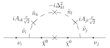
Figure 1: Radiative diagram at one loop level which generates Majorana neutrino mass.

The insertion of L-violating sneutrino masses allows the entry of radiative mass terms via the loop diagram shown in Fig. 1. The expression for the loop-induced contribution is

$$[m_{\nu}^{r}]_{ij} = -(A_{ik}\Delta_{kl}^{2}A_{jl})\frac{v^{2}}{2}\frac{g^{2}}{384\pi^{2}}\frac{1}{\tilde{m}^{5}}$$ (33)

$$= \frac{g^{2}}{384\pi^{2}}\frac{A^{4}\langle x_{ij}\rangle}{M_{P}}\frac{v^{2}}{2}\frac{1}{\tilde{m}^{5}}.$$

where $\tilde{m}$ is the SUSY breaking scale in the observable sector and is of the same order as the physical neutralino and sneutrino masses. The origin of the parameter $A$ in this scenario has been shown in equation 8. It is sufficient for us to assume $\langle x_{ij}\rangle=\langle x_{ji}\rangle$ and $A=A_{i}=F_{i}/M_{p}=F/M_{P}$ for all $i,j$, which makes each of the above matrices symmetric in $i,j$. With this choice and after making the transformation $\nu\rightarrow i\nu$ so as to change the overall sign of the neutrino mass term, the seesaw and radiative mass matrices respectively become

$$m_{\nu}^{s}=\frac{v^{2}}{4M_{P}}\frac{1}{F}\left(\begin{array}[]{ccc}\langle x_{12}\rangle^{2}+\langle x_{13}\rangle^{2}&\langle x_{13}\rangle\langle x_{23}\rangle&\langle x_{12}\rangle\langle x_{23}\rangle\\ \langle x_{13}\rangle\langle x_{23}\rangle&\langle x_{12}\rangle^{2}+\langle x_{23}\rangle^{2}&\langle x_{12}\rangle\langle x_{13}\rangle\\ \langle x_{12}\rangle\langle x_{23}\rangle&\langle x_{12}\rangle\langle x_{13}\rangle&\langle x_{13}\rangle^{2}+\langle x_{23}\rangle^{2}\end{array}\right).$$ (37)

$$m_{\nu}^{r}=-\frac{g^{2}}{384\pi^{2}}\frac{F^{4}}{M^{5}_{P}}\frac{v^{2}}{2\tilde{m}^{5}}\left(\begin{array}[]{ccc}0&\langle x_{12}\rangle&\langle x_{13}\rangle\\ \langle x_{12}\rangle&0&\langle x_{23}\rangle\\ \langle x_{13}\rangle&\langle x_{23}\rangle&0\end{array}\right).$$ (41)

In the above expressions we have used $A=\frac{F}{M_{P}}$. The uncertainty in $m_{\nu}^{s}$ caused by running down to the electroweak scale can be absorbed in $\langle x_{ij}\rangle$ and $F$, since we are concerned with only the orders of magnitude of the latter. Also, the masses of all superparticles such as neutralinos and sneutrinos have been clubbed together as $\tilde{m}$ here. With such an approximation already made, the effect of renormalization group evolution is not expected to make much difference. Finally, with the effects of both nonrenormalizable interactions and lepton-number violation, taken into account, our most general neutrino mass matrix is

$$m_{\nu}=m_{\nu}^{s}+m_{\nu}^{r}.$$ (42)

Comparing the above mass matrix with Eq. (3), we are led to the following equations in the notation of section 2.

$$m_{1}c^{2}+m_{2}s^{2} = \frac{v^{2}}{4M_{P}}\frac{1}{F}(\langle x_{12}\rangle^{2}+\langle x_{13}\rangle^{2})$$ (43)

$$\frac{1}{2}(m_{1}s^{2}+m_{2}c^{2}+m_{3}) = \frac{v^{2}}{4M_{P}}\frac{1}{F}(\langle x_{12}\rangle^{2}+\langle x_{23}\rangle^{2})$$ (44)

$$= \frac{v^{2}}{4M_{P}}\frac{1}{F}(\langle x_{13}\rangle^{2}+\langle x_{23}\rangle^{2})$$ (45)

$$\frac{cs}{\sqrt{2}}(-m_{1}+m_{2}) = -\frac{g^{2}}{384\pi^{2}}\frac{F^{4}}{M^{5}_{P}}\frac{v^{2}}{2\tilde{m}^{5}}\langle x_{12}\rangle+\frac{v^{2}}{4M_{P}}\frac{1}{F}\langle x_{13}\rangle\langle x_{23}\rangle$$ (46)

$$\frac{cs}{\sqrt{2}}(m_{1}-m_{2}) = -\frac{g^{2}}{384\pi^{2}}\frac{F^{4}}{M^{5}_{P}}\frac{v^{2}}{2\tilde{m}^{5}}\langle x_{13}\rangle+\frac{v^{2}}{4M_{P}}\frac{1}{F}\langle x_{12}\rangle\langle x_{23}\rangle$$ (47)

$$\frac{1}{2}(-m_{1}s^{2}-m_{2}c^{2}+m_{3}) = -\frac{g^{2}}{384\pi^{2}}\frac{F^{4}}{M^{5}_{P}}\frac{v^{2}}{2\tilde{m}^{5}}\langle x_{23}\rangle+\frac{v^{2}}{4M_{P}}\frac{1}{F}\langle x_{12}\rangle\langle x_{13}\rangle$$ (48)

One set of consistent solutions to equations (25),(26) and (27),(28) is $\langle x_{12}\rangle=-\langle x_{13}\rangle$. This reduces the above six equations to four which can be expressed as follows:

$$m_{1}=\frac{v^{2}}{2M_{P}}\frac{|\langle x_{12}\rangle|^{2}}{F},\qquad m_{2} = \frac{v^{2}}{2M_{P}}\frac{|\langle x_{12}\rangle|^{2}}{F},\qquad m_{3}=\frac{v^{2}}{2M_{P}}\frac{|\langle x_{23}\rangle|^{2}}{F},\qquad$$

$$\tilde{m}^{5} = \frac{2g^{2}}{384\pi^{2}}\frac{F^{5}}{M^{4}_{P}}\frac{1}{|\langle x_{23}\rangle|}$$ (49)

The last two of the above equations can be combined to eliminate $\langle x_{23}\rangle$ and yield

$$\tilde{m}^{5}=\frac{\sqrt{2}g^{2}}{384\pi^{2}}\frac{F^{5}}{M^{4}_{P}}\frac{v}{\sqrt{m_{3}M_{P}F}},$$ (50)

a form that will be used in our numerical analysis.

It is remarkable that the angle $\theta_{12}$ does not arise in Eq. (30). In the left hand sides of Eqs. (24)$-$(29) we have three independent neutrino mass eigenvalues and there are three independent parameters on the corresponding right hand sides. The three parameters can be expressed as:

$$\chi_{1}=\frac{|\langle x_{12}\rangle|}{\sqrt{F}},\quad\chi_{2}=\frac{|\langle x_{23}\rangle|}{\sqrt{F}},\quad\chi_{3}=\frac{F^{9/2}}{\tilde{m}^{5}M^{4}}.$$ (51)

Upon using the relation $\langle x_{12}\rangle=-\langle x_{13}\rangle$ in Eqs. (24)$-$(29), we are left with four equations. Any three of them can be used to solve $\chi_{1}$, $\chi_{2}$ and $\chi_{3}$ in terms of $m_{1}$, $m_{2}$, $m_{3}$, $c$ and $s$. On substituting the values of the $\chi$’s in the fourth equation, we obtain a constraint equation among $m_{1}$, $m_{2}$, $m_{3}$, $c$ and $s$. The latter is automatically satisfied for $m_{1}=m_{2}$ irrespective of the value of $\theta_{12}$. Thus the near-equality of two mass eigenvalues, basically reflecting the smallness of the mass splitting required by the solar neutrino deficit (as compared to that necessitated by the atmospheric neutrino shortfall), causes $\theta_{12}$ to disappear from the solutions.

The above feature can perhaps be motivated by symmetries of the neutrino mass matrix. As has been noted in recent works [17], when one sets $\theta_{23}=\pi/4$, $\theta_{13}=0$, and further neglects the mass splitting $m_{2}-m_{1}$, then the mass matrix becomes invariant under the successive interchange of the second and third rows, and the second and third columns. This symmetry is found to be independent of the value of $\theta_{12}$: a feature to which the observations of the previous paragraph can be related.

3.4 Constraint from $\mu\to e\gamma$

Special care has been taken in our formulation to ensure a diagonal form for $F_{X_{ij}}$ so that FCNC processes are suppressed. However, a strongly constrained process like the radiative leptonic decay $\mu\to e\gamma$ can still receive one-loop contributions via two insertions of the L-violating sneutrino mass, as shown in Fig. 2.

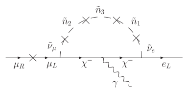
Figure 2: $\mu\to e\gamma$, an FCNC process is shown at one loop level.

In order to estimate such a contribution, one can compute the corresponding amplitude:

$$A^{\mu}\sim\frac{eg^{2}V^{(e)}V^{(\mu)}}{16\pi^{2}\times 30\tilde{m}}\left(\frac{\langle x\rangle}{M_{P}}\right)^{2}\bar{u}(p^{\prime})\left(\frac{1+\gamma_{5}}{2}\right)(\sigma^{\mu\nu}q_{\nu})u(p),$$ (52)

where $p,p^{\prime}$ are momenta of the incoming muon and the outgoing electron in Fig. 2 and $q=p^{\prime}-p$. Here $V^{(e)},V^{(\mu)}$ are summed mixing matrix elements that enter the corresponding chargino-lepton-sneutrino vertices. In the above equation we have used $A\sim M_{EW}\sim\tilde{m}$. By comparing this expression with, say the Standard Model amplitude for the $\mu\to e\gamma$ transition, we notice that there is an additional suppression factor of $\left(\frac{\langle x\rangle}{M_{P}}\right)^{2}\sim 10^{-7}$. This factor is small enough to automatically ensure a sufficiently low rate for the process $\mu\to e\gamma$.

4 Different scenarios of neutrino mass hierarchy

From the four equations (30), we notice that low-energy observables are ultimately controlled by three parameters of the model, namely, $|\langle x_{12}\rangle|,|\langle x_{23}\rangle|$ and $F$. In order to fix them (or the ranges they lie in), though, one needs to know the values of the neutrino masses, along with the mixing angles. However, while the mixing angles are experimentally known to be in certain allowed ranges, all that we can claim to know so far about the masses are the mass-squared differences $\Delta m^{2}_{12}$ and $|\Delta m^{2}_{23}|$, corresponding to the solar and atmospheric neutrino deficits respectively. Their allowed ranges of values, together with those of the mixing angles, can be found, for example, in [10]. Based on these ranges, all three scenarios, namely, normal hierarchy, inverted hierarchy and degenerate masses [18], can be constructed in our model. Each of these places the individual mass eigenvalues within specified ranges. On using them, one can obtain the allowed ranges of the model parameters mentioned above. In the process, simultaneous use can be made of the fact that the SUSY breaking mass parameter $\tilde{m}$ is bounded from above if there are observable TeV-scale superparticles. Similarly, a lower bound on $\tilde{m}$ can be imposed from negative superparticle searches with present accelerator data. Using the expression for $\tilde{m}$, the allowed space for the VEVs of the components of the gauge singlet chiral superfields can be further constrained. Thus one can check whether the VEVs of the scalar and auxiliary components of the $X_{ij}$, as required by neutrino masses, are consistent with the expected scale of SUSY breaking and the value of the $\mu$-parameter. The self- consistency of the entire scheme gets established in this way.

For illustration, we take the lower and upper bounds on $\tilde{m}$ to be about 100 GeV and 2 TeV respectively. The allowed mass-squared difference ranges from oscillation data are

$$\Delta m^{2}_{21} = (8.0\pm 0.3)\times 10^{-5}{\rm eV}^{2}$$

$$|\Delta m^{2}_{32}| = (2.5\pm 0.3)\times 10^{-3}{\rm eV}^{2}.$$ (53)

We have taken $M_{P}=2\times 10^{18}$ GeV in our numerical analysis. The results presented below show the minimum value of $\sqrt{F}$ to be above $5\times 10^{9}$ Gev, corresponding to the lower limit on $\tilde{m}$, which has its justification in the Large Electron Positron (LEP) collider results.

4.1 Normal hierarchy

This scenario corresponds to

$$m_{1}\approx m_{2}\sim\sqrt{\Delta m^{2}_{21}},\qquad m_{3}\sim\sqrt{|\Delta m^{2}_{32}|}.$$ (54)

In figures 3(a),(b) we have shown the allowed regions in the $|\langle x_{12}\rangle|-\sqrt{F}$ and $|\langle x_{23}\rangle|-\sqrt{F}$ planes corresponding to the $3\sigma$ range of $\sqrt{\Delta m^{2}_{21}}$ as well as of $\sqrt{|\Delta m^{2}_{32}|}$. On using the lower and upper limits of $\tilde{m}$, mentioned earlier, $\sqrt{F}$ is found to range between $\approx~{}5\times 10^{9}$ GeV and $5\times 10^{10}$ GeV. The scalar VEVs, on the other hand, are found to lie in the range of $10^{11}$ $-$ $10^{12}$ GeV. Finally, in figure 3(c) we have plotted $\tilde{m}$ against $\sqrt{F}$ using Eq. (31) for the lower and upper limits of $m_{3}$ at the $3\sigma$ level. If $F$ has to be related to the SUSY breaking mass terms, it is desirable to have it in the high side of the allowed region shown here. Thus values of $F$ like a few times $10^{10}$ GeV, and therefore $\tilde{m}$ somewhat on the higher side of the permissible range, are therefore favored in this model, given the accelerator search limits on superparticles.

The next point to note is that while $m_{2}$ and $m_{3}$ have specific lower as well as upper limits in the normal hierarchy scenario, $m_{1}$ could, in principle, go down to zero. Nevertheless, the difference between $m_{1}$ and $m_{2}$ being quite small, the allowed region is restricted to be so narrow that it can be almost called fine-tuned. As discussed below, the situation is somewhat different in this respect in the case of inverted hierarchy.

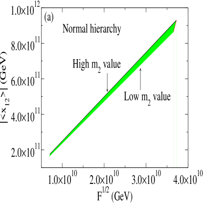
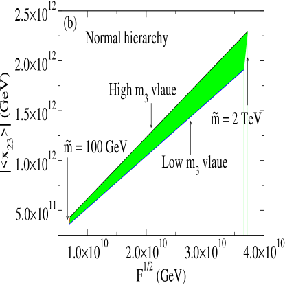
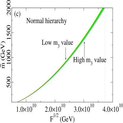
Figure 3: Normal hierarchy: the top left (right) panel shows the allowed region in the $|\langle x_{12}\rangle|(|\langle x_{23}\rangle|)-\sqrt{F}$ plane. The center lower panel shows the dependence of the SUSY mass scale $\tilde{m}$ on $\sqrt{F}$ in the allowed region of $m_{3}$.

4.2 Inverted hierarchy

Here we have

$$m_{1}\approx m_{2}\sim\sqrt{|\Delta m^{2}_{32}|},\qquad m_{3}\ll\sqrt{|\Delta m^{2}_{32}|}.$$ (55)

Notice that the relation $\sqrt{|\Delta m^{2}_{32}|}=\frac{v^{2}}{2M_{P}}\frac{|\langle x_{12}\rangle|^{2}}{F}$ gives us the same plot as figure 3(b), with $|\langle x_{23}\rangle|$ replaced by $|\langle x_{12}\rangle|$ in the y-axis. In addition, $|\langle x_{23}\rangle|$ is plotted against $\sqrt{F}$ in figure 4(a). Since we know that $\sqrt{|\Delta m^{2}_{32}|}\sim$ 0.05 eV, we have allowed a maximum of $m_{3}=0.01$ eV. The minimum value of $m_{3}$, on the other hand, could in principle be zero. In this case, too, for each $m_{3}$ value there is a limiting upper bound on $F$ coming because $\tilde{m}\leq$ 2 TeV. The corresponding parameter range is represented by the shaded area in figure 4(b), where $\tilde{m}$ is plotted against $\sqrt{F}$ using Eq. (31) upto a maximum value of $m_{3}=0.01$ eV starting from $m_{3}=0$. The interesting point to note here is that $m_{3}$ has no specified lower limit in this scenario. As a result, the allowed regions in the parameter space are much wider and less fine-tuned compared to the normal hierarchy scenario. Our conclusion, therefore, is that the inverted hierarchy scenario allows a larger flexibility of high-scale parameter combinations in the scheme adopted here.

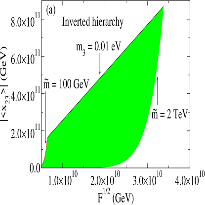
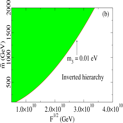
Figure 4: Inverted hierarchy: the left panel shows the allowed region in the $|\langle x_{23}\rangle|-\sqrt{F}$ plane. The right panel shows the variation of the SUSY mass scale $\tilde{m}$ against $\sqrt{F}$ in the allowed range of $m_{3}$.

4.3 Degenerate masses

This case corresponds to

$$m_{1}\approx m_{2}\approx m_{3}\gg\sqrt{|\Delta m^{2}_{23}|},$$ (56)

leading to $|\langle x_{12}\rangle|\approx|\langle x_{23}\rangle|$ along with the requirement the actual masses shoul be significantly greater than the mass-square separations. Since $\sqrt{|\Delta m^{2}_{32}|}\sim$ 0.05 eV, we have to take $m_{3}\gg 0.05$ eV. On the other hand, since these are Majorana neutrinos, there is an upper bound of about 0.3 eV on the lightest mass from neutrinoless double beta decay as well as from cosmological constraints [10]. Therefore, we have plotted $|\langle x_{12}\rangle|$ against $\sqrt{F}$ for $m_{2}$ ranging from 0.1 eV to $m_{2}$ = 0.3 eV, showing the allowed range as shaded area. This is shown in figure 5(a) with the usual constraints on $F$ coming from $\tilde{m}$. In figure 5(b), the allowed region in the $\tilde{m}$ $-$ $\sqrt{F}$ plane is shown with $m_{3}$ ranging between 0.1 eV and 0.3 eV.

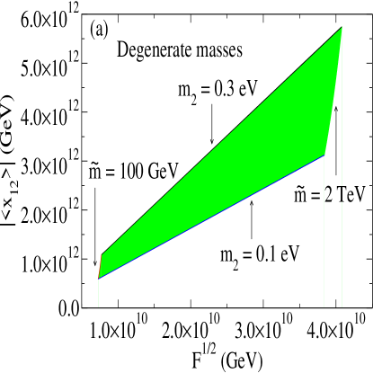
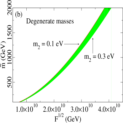
Figure 5: Degenerate masses: the left panel shows the allowed parameter space in the $|\langle x_{12}\rangle|-\sqrt{F}$ plane. The right panel shows the variation of the SUSY mass scale $\tilde{m}$ against $\sqrt{F}$ in the allowed range of $m_{3}$.

4.4 Overall observations

After analyzing these three cases, we can compare their impact on the parameters of our proposed model vis-a-vis the same on other similar models put forward in the literature. In the model considered in [3], for example, there is effectively one parameter which is $F\approx\langle x\rangle^{2}$. This is because just one right-chiral neutrino was considered there. That is why, despite the occurrence of both seesaw and radiative masses, the former are negligibly small in magnitude as compared to the latter. We have a more general (and natural) picture with three right-chiral neutrino superfields. There are consequently three unconnected parameters $F,|\langle x_{12}\rangle|$ and $|\langle x_{23}\rangle|$. These give us more freedom enabling us to treat the seesaw and the radiative masses on the same footing. The plots shown above for the three different neutrino mass cases imply that the different parameters which enter are in the expected range, thereby demonstrating the self-consistency of our model.

It should be noted that the SUSY breaking scale $\tilde{m}$ is related to $F$ by the relation $\tilde{m}\sim\frac{F}{M_{P}}$, and that they are not entirely independent. The results presented in figures 3$-$5 confirm that such a dependence is consistent with the requirement of neutrino masses and mixing. Some additional constraints may be required; for example, for $\tilde{m}$ on the higher side, one may be restricted to relatively larger values of $F$. However, it is impossible to be more exact in the absence of precise knowledge of the coupling strengths and other numerical factors in the hidden sector. Naively, eq. (31) is consistent with $\tilde{m}\sim\frac{F}{M_{P}}$ for $m_{3}$ in the range .01 $-$ .1 eV. This, in principle, restricts the inverted hierarchy scenario a little bit, although it is difficult to be very precise, for reasons already mentioned.

It is clear from the expression of Eq. (30) for $\tilde{m}$ that our model connects very light neutrinos to TeV-scale massive particles. The latter include superparticles such as neutralinos and sneutrinos as well as right-chiral neutrinos. Further experimental information on neutrino masses, specifically the fixation of the hierarchy scenario, will therefore enable us to indirectly probe such yet undiscovered particles. At the same time, we have guidelines concerning the SUSY breaking sectors, especially the non-renormalizable terms that may have other ramifications such as explaining the worrisome $\mu$-problem.

5 Other possibilites

In this section we briefly comment on two other representative scenarios where nonrenormalizable interactions may be invoked to explain the observed pattern in the neutrino sector. We emphasize, however, that none of these has any bearing on the conclusions presented in the last two sections. We include these remarks mainly for the sake of completeness.

In $\S 3.2$ we presented a superpotential which led us to diagonal A-terms and the consequent suppression of FCNC effects. This requires nonvanishing F-component VEVs only for the diagonal elements of the array of superfields $X_{ij}$; the nondiagonal members of the array should have VEVs of the scalar components only, in order to generate off-diagonal elements of the neutrino mass matrix. One may be curious to ask whether, for the diagonal elements $X_{ii}$, one can have nonvanishing VEVs for both the scalar and the auxiliary components and if such be the case, what their implications should be.

There are some models based on Polonyi fields in which SUSY breaking has been achieved with a vanishing cosmological constant  [15]. In these supergravity-inspired models, on integrating out some additional chiral quark fields at a scale $\Lambda$, an effective superpotential

$$W=\lambda\Lambda^{2}Z$$ (57)

is obtained at a scale below $\Lambda$. Here $\lambda$ is a constant ${\cal O}$(1) and $Z$ is a Polonyi superfield. The scalar potential constructed therefrom yields $\langle F_{Z}\rangle=\lambda\Lambda^{2}$. At the same time, supergravity effects lift the flatness of the direction $\langle z\rangle=0$ so that both the scalar and auxiliary components of the chiral superfield $Z$ have nonvanishing VEVs.

Though one has in the past appealed to such models  [2, 3, 4], they do pose some difficulties in our case. A superpotential of the above kind cannot be used for off-diagonal elements of $X_{ij}$, since those would generate large $A_{ij}$’s for $i\neq j$ and threaten to enhance FCNC rates. Thus the superpotentials for the diagonal and off-diagonal members would look very different in such a case, thereby raising doubts about the legitimacy of using the components of $X_{ij}$ as fields of a similar type. What we have done, on the other hand, does not raise such questions, since the complementarity of $\langle x_{ij}\rangle$ and $F_{X_{ij}}$ is decided essentially by the relative magnitudes of two sets of mass parameters ($\mu$, $\mu^{\prime}$) of the same order, where some fluctuation is quite natural.

Another possibility [3] lies in considering the effective SUSY Lagrangian

$${\cal L}_{eff}=[XNN+LNH_{u}]_{F}+{\rm h.c.},$$ (58)

having one right-chiral neutrino to explain tiny neutrino masses. Eq. (39) can be readily generalized to include three right-chiral neutrinos, i.e.

$${\cal L}_{eff}=[X_{ij}N^{i}N^{j}+\lambda_{i}\delta_{ij}L^{i}N^{j}H_{u}]_{F}+{\rm h.c.},$$ (59)

where there is a summation over the flavor indices $i,j$ and $\lambda_{i}$ are Yukawa couplings. The Kronecker $\delta$ in the second term is to suppress FCNC processes. This Lagrangian can be justified on the basis of the global symmetry $G_{F}\times G$, where $G_{F}=SO(3)_{F}$ and $G=U(1)_{R}\times U(1)_{L}$. For SUSY breaking, consider the hidden sector superpotential

$$W=\sum_{i,j=1}^{3}W_{ij},$$ (60)

where

$$W_{ij}=S_{ij}(X_{ij}\bar{X}_{ij}-\mu^{2}_{ij})+\bar{X}^{2}_{ij}Y_{ij}+X^{2}_{ij}\bar{Y}_{ij}.$$ (61)

The charges for various fields under $G$ in this case are:

$$S_{ij}(2,0),\quad X_{ij}(0,2),\quad\bar{X}_{ij}(0,-2),\quad Y_{ij}(2,4),$$ (62)

$$\bar{Y}_{ij}(2,-4),\quad N^{i}(1,-1),\quad L^{i}(1,1),\quad H_{u}(0,0),\quad H_{d}(0,0).$$

The minimization of the scalar potential, arising from this superpotential, yields $\langle x_{ij}\rangle\neq 0$ for all $i,j$. After SUSY breaking, Dirac and right-handed neutrino masses are generated as

$$[m_{D}]_{ij}=\frac{v}{\sqrt{2}}\lambda_{i}\delta_{ij},\qquad[m_{R}]_{ij}=\langle x_{ij}\rangle.$$ (63)

Hence the seesaw mass is

$$m_{\nu}=-m_{D}m_{R}^{-1}m_{D}^{T}.$$ (64)

For $\langle x_{ij}\rangle\sim 10^{11}$ GeV and $\lambda_{i}\sim$ 0.01, we obtain neutrino masses $m_{\nu}\sim$ 0.1 eV. Following the analysis given in the earlier sections, we can explain the observed bilarge neutrino mixing as well as different hierarchies in some parameter space of $\langle x_{ij}\rangle$. However, no connection can be made in this scenario between the tiny neutrino masses and the TeV-scale particles of MSSM. This is since only $\langle x\rangle$ enters the game and no $\langle F\rangle$. Moreover, a global symmetry of the form $U(1)_{R}\times U(1)_{L}$ does not allow the triple-$X$ higher order term which can generate the $\Delta L=2$ sneutrino mass, cf. Eq. (9), in this particular model. Thus there can be no radiative contribution, at least not in the lowest orders. So one is unable to use here the full potential of such a scenario which, in our case, has meant a considerable widening of the parameter space through an interplay of seesaw and radiative effects, making our model more accommodating and natural.

6 Summary and conclusion

With a broken supersymmetric theory, we have considered a general scenario where the neutrino mass matrix is constructed through a combination of the seesaw mechanism and radiative effects. All the agents behind the mechanism for this generation come from (a) a sector containing nonrenormalizable interactions in the superpotential and (b) lepton-number violating terms. We have used an array of gauge singlet chiral superfields $X_{ij}$ for this purpose. In terms of these, we have constructed a superpotential which allows both the above types of contributions, while ensuring FCNC suppression. Right-chiral sneutrinos are found to have as much of a role in the process as the corresponding neutrinos. It should be noted that the angle $\theta_{13}$ vanishes on using the bilarge mixing matrix in equation 2. A small but nonvanishing value of $\theta_{13}$ requires one to modify equations (24)$-$(29), although no quatitative change in the conclusions is expected. We have then taken in turn the neutrino mass scenarios of normal hierarchy, inverted hierarchy and degenerate neutrinos. Using the masses answering to each scenario, we have traced out the allowed region of the parameter space of the involved high-scale physics, given in terms of the relevant VEVs of the scalar and auxiliary components of the superfields $X_{ij}$. Numerically, these are seen to allow a self-consistent region of the parameter space. While the scenario of normal hierarchy (and, partly, that of degenerate neutrinos) forces us into somewhat fine-tuned zones of the parameter space, the inverted hierarchy picture allows a considerably larger region. With forthcoming laboratory measurements and cosmological observations hopefully deciding among the above mass patterns, connecting experimental observables to high-scale physics may become a realistic proposition, especially if Nature indeed proves to be supersymmetric.

Acknowledgment: PR acknowledges the hospitality of Harish-Chandra Research Institute where this work was initiated. RS wishes to thank the Department of Theoretical Physics, Tata Institute of Fundamental Research, for its hospitality during the progress of this work.

References

- [1] For reviews see, for example, G. Altarelli and F. Feruglio, arXiv:hep-ph/0206077; New J. Phys 6, 106 (2004); B. Mukhopadhyaya, arXiv: hep-ph/0301278, and references therein.
- [2] N. Arkani-Hamed, L. Hall, H. Murayama, D. Smith and N. Weiner, Phys. Rev. D 64, 115011 (2001).
- [3] N. Arkani-Hamed, L. Hall, H. Murayama, D. Smith and N. Weiner, arXiv:hep-ph/0007001.
- [4] F. Borzumati and Y. Nomura, Phys. Rev. D 64, 053005 (2001).
- [5] C.D. Froggatt and H.B. Nielsen, Nucl. Phys. B147, 277 (1979).
- [6] R.N. Mohapatra and S. Nussinov, Phys. Lett. B 441, 299 (1998); R.N. Mohapatra and S. Nussinov, Phys. Rev. D 60, 013002 (1999); R. Kuchimanchi and R.N. Mohapatra, Phys. Rev. D 66, 051301(R) (2002); E. Ma, arXiv:hep-ph/0508099, ibid.hep-ph/0508231.
- [7] L. Hall, H. Murayama and N. Weiner, Phys. Rev. Lett. 84, 252 (2002); N. Haba and H. Murayama, Phys. Rev. D 63, 053010 (2001); A. de Govea and H. Murayama, Phys. Lett. B 573, 94 (2003); G. Altarelli and F. Feruglio, J. High Energy Phys. 0301, 035 (2003).
- [8] D.N. Spergel et al., Astrophys. J. Suppl., 148, 175 (2003); O. Elgaroy and O. Lahav, JCAP 0304, 004 (2003); S. Hannestad, JCAP 0305, 004 (2003); S.W. Allen, R.W. Schmidt and S.L. Bridle, Tsukuba 2003, Cosmic Ray, p 1921, arXiv:astro-ph/0306368.
- [9] H.V. Klapdor-Kleingrothaus et al., Eur. Phys. J. A 12, 147 (2001); A.M. Bakalyarov et al., Phys. Part. Nucl. Lett. 2, 77 (2005); H.V. Klapdor-Kleingrothaus et al., Mod. Phys. Lett. A 16, 2409 (2001).
- [10] A. Strumia and F. Vissani, Nucl. Phys. B726, 294 (2005).
- [11] L. Wolfenstein, Phys. Rev. D 17, 2369 (1978); S.P. Mikheyev and A. Yu. Smirnov, Yad. Fiz. 42, 1441 (1985); Nuovo Cim. C 9, 17 (1986); Sov. Phys. JETP, 64, 4 (1986).
- [12] SNO collaboration (S. N . Ahmed et al.), Phys. Rev. Lett. 92, 181301 (2004); K. Eguchi et al., (KamLAND), Phys. Rev. Lett. 90, 021802 (2003).
- [13] M. Maltoni, T. Schwetz, M.A. Tortola and J.W.F. Valle, New J. Phys. 6, 122 (2004).
- [14] M. Apollonio et al., Phys. Lett. B 466, 415 (1999); A. Bandyopadhyay, S. Choubey, S. Goswami, S.T. Petcov and D.P. Roy, Phys. Lett. B 583, 134 (2004); P.C. de Holanda and A. Yu. Smrinov, Astropart. Phys. 21 (2004); G.L. Fogli et al., Phys. Rev. D 69, 017301 (2004).
- [15] I. Ken-Iti and T. Yanagida, Prog. Theor. Phys. 94, 1105 (1995), ibid. 95, 829 (1996).
- [16] For earlier works on masses of right-chiral sneutrinos see, for example, G. D’ Ambrosio, G. Giudice and M. Raidal, Phys. Lett. B 575, 75 (2003); Y. Grossman, T. Kashti, Y. Nir, E. Roulet, J. High Energy Phys. 0411, 080 (2004); Y. Grossman, T. Kashti, Y. Nir, E. Roulet, Phys. Rev. Lett., 91, 251801 (2003).
- [17] C.S. Lam, Phys. Rev. D 71, 093001 (2005).
- [18] A. Joshipura, Proceedings of the Indian National Science Academy, 70A, 223 (2004).