Hadronic corrections to muon anomalous magnetic moment within the instanton liquid model

Abstract

The current status of the muon anomalous magnetic moment problem is briefly presented. The corrections to muon anomaly coming from the effects of hadronic vacuum polarization, $Z^{\ast}\gamma\gamma^{\ast}$ effective vertex and light-by-light scattering are estimated within the instanton model of QCD vacuum.

13.40.Em, 14.60.Ef

1 Muon AMM: experiment vs theory.

The study of anomalous magnetic moments (AMM) of leptons, $a=(g_{S}-2)/2$, have played an important role in the development of the standard model (SM). At present accuracy the electron AMM due to small electron mass is sensitive only to quantum electrodynamic (QED) contributions. The theoretical error [1] is dominated by the uncertainty in the input value of the QED coupling $\alpha\equiv e^{2}/(4\pi)$. Thus, the electron AMM provides the best observable for determining the fine coupling constant

$$\alpha^{-1}=137.035~{}998~{}83(51).$$ (1)

Compared to the electron, the muon AMM has a relative sensitivity to heavier mass scales which is typically proportional to $\left(m_{\mu}/m_{e}\right)^{2}$. At present level of accuracy, the muon AMM gives an experimental sensitivity to virtual $W$ and $Z$ gauge bosons as well as a potential sensitivity to other, as yet unobserved, particles in the few hundred GeV$/c^{2}$ mass range. The muon AMM is known to an unprecedented accuracy of order of $1$ ppm. The latest result from the measurements of the Muon $(g-2)$ collaboration at Brookhaven is [2]

$$a_{\mu}^{\mathrm{Exp}}\equiv{\frac{1}{2}}(g_{\mu}-2)=11\ 659\ 208\left(6\right)\cdot 10^{-10},$$ (2)

which is the average of the measurements of the AMM for the positively and negatively charged muons (Fig. 1). In future, one expects to achieve more than a factor of $2$ reduction in $a_{\mu}$ uncertainty in planning BNL E969 experiment [3] and even more precise g-2 experiment is discussed in J-PARC with the proposal to reach a precision below $0.1$ ppm [4].

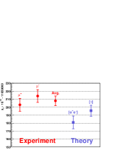
Figure 1: Measurements of $a_{\mu}$ by E821 (g-2) Collaboration with the SM predictions [2]. (Theoretical point based on usage of $e^{+}e^{-}\rightarrow$hadrons annihilation data is raised up after recent analysis by SND collaboration [5]).

The standard model prediction for $a_{\mu}$ consists of quantum electrodynamics, weak and hadronic contributions (schematically presented in Fig. 2). The QED and weak contributions to $a_{\mu}$ have been calculated with great accuracy [1]

$$a_{\mu}^{\mathrm{QED}}=11~{}658~{}471.935(0.203)\cdot 10^{-10}$$ (3)

and [6]

$$a_{\mu}^{\mathrm{EW}}=15.4(0.3)\cdot 10^{-10}.$$ (4)

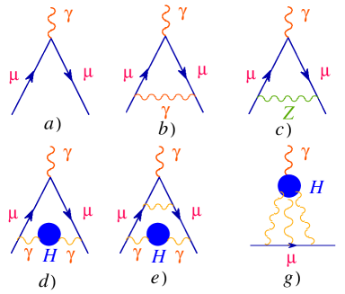
Figure 2: The standard model contributions to the muon anomalous magnetic moment.

The uncertainties of the SM value for $a_{\mu}$ (Fig. 1) are dominated by the uncertainties of the hadronic contributions, $a_{\mu}^{\mathrm{Strong}},$ since their evaluation involve quantum chromodynamics (QCD) at long-distances for which perturbation theory cannot be employed. Under assumption that at reached scales there are no New Physics effects one may estimate the hadronic part of the muon AMM by subtracting the QED and EW contributions from the experimental result (2)

$$a_{\mu}^{\mathrm{Strong(Exp)}}=721(6)\cdot 10^{-10}.$$ (5)

Below we discuss with some details theoretical status of hadronic contributions. First, we discuss the phenomenological estimates of the leading of order $\alpha^{2}$ (LO) hadronic corrections based on usage of inclusive $e^{+}e^{-}\rightarrow$hadrons and hadronic $\tau$ decays data. Then, one evaluate the hadronic corrections of leading and next-to-leading (NLO) order to muon AMM within the instanton liquid model of QCD vacuum (ILM).

2 Phenomenological estimates of the LO hadronic contributions to muon AMM

The LO contribution to the muon AMM comes from the hadronic vacuum polarization (Fig. 2d) and NLO corrections consisting of contributions which are the iteration of the LO term (Fig. 2e) plus the independent contribution from the light-by-light scattering process (Fig. 2g). In absolute value the LO and NLO terms differ by one order of magnitude, but the theoretical accuracy of their extraction is comparable and dominates the overall theoretical error of the SM calculations. All hadronic contributions are sensitive to the low energy physics and there are no rigorous theoretical methods based on first principles for the calculations. Thus, to confront usefully theory with the experiment requires a better determination of the hadronic contributions.

The LO correction to muon AMM, $a_{\mu}^{\mathrm{hvp}~{}\left(1\right)},$ is due to the hadronic photon vacuum polarization effect in the internal photon propagator of the one-loop diagram (Fig. 2d). Using analyticity and unitarity (the optical theorem) $a_{\mu}^{\mathrm{hvp}~{}\left(1\right)}$ can be expressed as the spectral representation integral [7, 8]

$$a_{\mu}^{\mathrm{hvp}\left(1\right)}=\left(\frac{\alpha}{\pi}\right)^{2}\int_{0}^{\infty}dt\frac{1}{t}K(t)\rho_{\mathrm{V}}^{(\mathrm{H})}\left(t\right)\ ,$$ (6)

which is a convolution of the hadronic spectral function $\rho_{V}^{\mathrm{(H)}}\left(t\right)$ with the known QED kinematical factor

$$K(t)=\int_{0}^{1}dx{\frac{x^{2}(1-x)}{x^{2}+(1-x)t/m_{\mu}^{2}}}\ ,$$ (7)

where $m_{\mu}$ is the muon mass. The QED factor is sharply peaked at low $t$ and decreases monotonically with increasing $t$. Thus, the integral defining $a_{\mu}^{\mathrm{hvp}\left(1\right)}$ is sensitive to the details of the spectral function $\rho_{V}^{\mathrm{(H)}}\left(t\right)$ at low invariant masses.

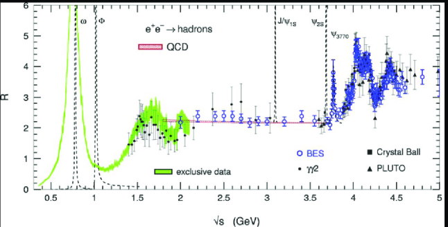
Figure 3: Spectral density as measured from $e^{+}e^{-}\rightarrow$hadrons annihilation, $R(s)=\sigma^{e^{+}e^{-}\rightarrow\mathrm{hadrons}}(s)/\sigma^{e^{+}e^{-}\rightarrow\mu^{+}\mu^{-}}(s)$.

At present there is no direct theoretical tools that allow to calculate the spectral function with required accuracy. Fortunately, $\rho_{V}^{\mathrm{(H)}}\left(t\right)$ is related to the total $e^{+}e^{-}\rightarrow\gamma^{\ast}\rightarrow$ hadrons cross-section $\sigma(t)$ by $(m_{e}\rightarrow 0)$

$$\sigma^{e^{+}e^{-}\rightarrow\mathrm{hadrons}}(t)=4\pi\alpha^{2}\frac{1}{t}\rho_{\mathrm{V}}^{(\mathrm{H})}\left(t\right),$$ (8)

and this fact is normally used to get quite accurate estimate of $a_{\mu}^{\mathrm{hvp}\left(1\right)}$. The condensed form accumulating the data of different experiments on the hadronic $e^{+}e^{-}$ annihilation is presented in Fig. 3. Moreover, high precision inclusive hadronic $\tau$ decay data [9, 10, 11] are used in order to improve the determination of $a_{\mu}^{\mathrm{hvp}\left(1\right)}$. This is possible, since the vector current conservation law relates the $I=1$ part of the electromagnetic spectral function to the charged current vector spectral function measured in $\tau\rightarrow\nu$ +non-strange hadrons. At present, it is found consistence within the experimental errors between $e^{+}e^{-}$ and $\tau$ data [5] (see Fig. 4). All these allows to reach during the last decade a substantial improvement in the accuracy of the contribution from the hadronic vacuum polarization.

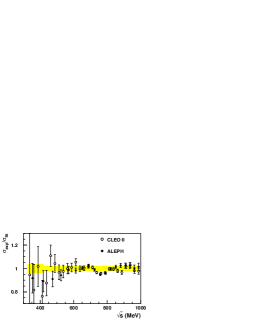
Figure 4: The ratio of the $e^{+}e^{-}\rightarrow\pi^{+}\pi^{-}$ cross section calculated from the $\tau^{-}\rightarrow\pi^{-}\pi^{0}\nu_{\tau}$ decay spectral function measured in [11, 9] to the isovector part of the $e^{+}e^{-}\rightarrow\pi^{+}\pi^{-}$ cross section measured by SND (from [5]). The shaded area shows the joint systematic error.

About 91% of $a_{\mu}^{\mathrm{hvp}\left(1\right)}$ comes from $t<(1.8$ GeV$)^{2}$, while 73% of the corresponding integral is covered by final $2\pi$ state. The most recent estimates of the dispersion integral for the $2\pi$-channel in the energy range $0.39<t_{\pi}<0.97$ GeV² which are based on the $e^{+}e^{-}$ experimental results are following

$$a_{\mu}^{\mathrm{\pi\pi}} =(378.6\pm 5.0)\cdot 10^{-10}\quad\mathrm{CMD2}\text{ }(2003)\cite[cite]{[\@@bibref{}{CMD2}{}{}]},$$

$$a_{\mu}^{\mathrm{\pi\pi}} =(375.6\pm 5.7)\cdot 10^{-10}\quad\mathrm{KLOE}\text{ }(2004)\cite[cite]{[\@@bibref{}{KLOE}{}{}]},$$

$$a_{\mu}^{\mathrm{\pi\pi}} =(385.6\pm 5.2)\cdot 10^{-10}\quad\mathrm{SND}\text{ }(2005)\cite[cite]{[\@@bibref{}{SND}{}{}]}.$$ (9)

The contributions of hadronic vacuum polarization at order $\alpha^{2}$ quoted in the theoretical articles on the subject are given in the Table 1. However, these analysis do not take into account recent SND data which alone may increase the estimates based on $e^{+}e^{-}$ annihilation by approximately $(7\div 10)\cdot 10^{-10}$ (see (9)) making $e^{+}e^{-}$ and $\tau$ data analysis more consistent from one side and more close to experimental result from other one.

Table 1.
Phenomenological estimates and references for the leading order hadronic photon vacuum polarization contribution to the muon anomalous magnetic moment based on $e^{+}e^{-}$ and $\tau$ data sets.

	$e^{+}e^{-}\cite[cite]{[\@@bibref{}{DEHZh03}{}{}]}$	$\tau\cite[cite]{[\@@bibref{}{DEHZh03}{}{}]}$	$e^{+}e^{-}\cite[cite]{[\@@bibref{}{J}{}{}]}$	$e^{+}e^{-}\cite[cite]{[\@@bibref{}{TrocYnd}{}{}]}$	$\tau\cite[cite]{[\@@bibref{}{TrocYnd}{}{}]}$
$a_{\mu}^{\mathrm{hvp}~{}\left(1\right)}\cdot 10^{10}$	$696.3\pm 9.8$	$711.0\pm 8.6$	$694.8\pm 8.6$	$693.5\pm 9.0$	$701.8\pm 8.9$

The higher order hadronic corrections to $a_{\mu}$ are schematically presented in Figs. 2 e and g. These diagrams, like leading order contribution, cannot be calculated in perturbative QCD, but part of them may be estimated with help of experimental data on inclusive hadronic $e^{+}e^{-}$ annihilation and $\tau$ decays as [17]

$$a_{\mu}^{\mathrm{hvp}\left(2\right)}=-10.1(0.6)\cdot 10^{-10}.$$ (10)

This, however, not the case for the so called light-by-light contribution, $a_{\mu}^{\mathrm{h.~{}L\times L}}$, (Fig. 2g) where one needs to explore the QCD motivated approaches. The latter has been estimated recently using the vector meson dominance model supplemented by perturbative QCD constraints [20]

$$a_{\mu}^{\mathrm{h.~{}L\times L}}=13.6(2.5)\cdot 10^{-10}.$$ (11)

The agreement between the SM predictions and the present experimental values is rather good. There is certain inconsistencies in use of different sets of experimental data based on the $e^{+}e^{-}$ and $\tau$ processes in evaluations of the LO hadronic contribution to the muon AMM. The analysis based on the $\tau$ decay data and recent $e^{+}e^{-}$ data from SND collaboration [5] provide the SM results which are in good agreement with the experimental one. The results based on the $e^{+}e^{-}$ data published by the CMD [12] and KLOE [13] data support bigger difference between SM prediction and (g-2) Collaboration result. Theoretically, the $\tau$ decay data is found [21] to be more compatible with expectations based on high-scale $\alpha_{s}(M_{Z})$ determinations; the electroproduction data (CMD, KLOE), in contrast, requires significantly lower $\alpha_{s}(M_{Z})$. The results favor determinations of the leading order hadronic contribution to $a_{\mu}$ which incorporate hadronic $\tau$ decay data over those employing electroproduction data only, and hence suggest a reduced discrepancy between the SM prediction and the current experimental value of $a_{\mu}$.

3 The Adler function and $a_{\mu}^{\mathrm{hvp}\left(1\right)}.$

Recently, the isovector vector ($V)$ and axial-vector ($A)$ spectral functions have been determined separately with high precision by the ALEPH [9] and OPAL [10] collaborations from the inclusive hadronic $\tau$-lepton decays ($\tau\rightarrow\nu_{\tau}+$ hadrons) in the interval of invariant masses up to the $\tau$ mass, $0\leq s\leq m_{\tau}^{2}$. The vector spectral function measured by ALEPH is shown in Fig. 5. It is important to note that the experimental separation of the $V$ and $A$ spectral functions allows us to test accurately the saturation of the chiral sum rules of Weinberg-type in the measured interval. On the other hand, at large $s$ the correlators can be confronted with perturbative QCD (pQCD) thanks to sufficiently large value of the $\tau$ mass.

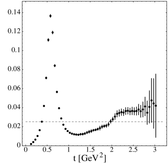
Figure 5: The isovector vector spectral function ($1/4\pi^{2})\rho_{V}(t)$ from hadronic $\tau$- decays [9]. The dashed line is the asymptotic freedom prediction, ($1/4\pi^{2}).$

Model estimates of the light quark strong sector of the standard model will be discussed in the chiral limit, when the masses of $u$, $d$, $s$ light quarks are set to zero. In this approximation, the $V$ and non-singlet $A$ current-current correlation functions in the momentum space (with $-q^{2}\equiv Q^{2}\geq 0$) are defined as

$$\Pi_{\mu\nu}^{J}(q) =i\int d^{4}x~{}e^{iqx}\Pi_{\mu\nu}^{J,ab}(x)=\,\left[\left(q_{\mu}q_{\nu}-g_{\mu\nu}q^{2}\right)\Pi_{J}(Q^{2})\right],$$ (12)

$$\qquad\Pi_{\mu\nu}^{J}(x) =\langle 0\left|T\left\{J_{\mu}(x)J_{\nu}(0)^{\dagger}\right\}\right|0\rangle,$$

where in the local theory the QCD $V$ and $A$ currents for light quarks are defined as

$$J_{\mu}=\bar{q}\,\gamma_{\mu}Vq,\qquad J_{\lambda}^{5}=\bar{q}\,\gamma_{\lambda}\gamma_{5}Aq\,,$$ (13)

the quark field $q_{f}^{i}$ has color ($i$) and flavor ($f$) indices, $A^{\left(3\right)}=\tau_{3}$ is the isospin matrix of the axial current, and $V=\frac{1}{2}\left(\frac{1}{3}+\tau_{3}\right)$ is the charge matrix. The momentum-space two-point correlation functions obey (suitably subtracted) dispersion relations,

$$\Pi_{J}(Q^{2})=\int_{0}^{\infty}\frac{ds}{s+Q^{2}}\frac{1}{\pi}\mathrm{Im}\Pi_{J}(s),$$ (14)

where the imaginary parts of the correlators determine the spectral functions

$$\rho_{J}(s)=4\pi\mathrm{\operatorname{Im}}\Pi_{J}(s+i0).$$ (15)

Instead of the polarization function it is more convenient to work with the Adler function defined as

$$D_{J}(Q^{2}){=-Q}^{2}\frac{d\Pi_{J}(Q^{2})}{dQ^{2}}{\,=}\frac{1}{4\pi^{2}}\int_{0}^{\infty}{dt}\frac{Q^{2}}{(t+Q^{2})^{2}}{\,\rho_{J}(t)\,.}$$ (16)

Then, it is possible to express $a_{\mu}^{\mathrm{hvp}\left(1\right)}$ given by (6) in terms of the Adler function by using the integral representation [22]

$$a_{\mu}^{\mathrm{hvp}\left(1\right)}=\frac{4}{3}\alpha^{2}\int_{0}^{1}dx\frac{\left(1-x\right)\left(2-x\right)}{x}D_{V}\left(\frac{x^{2}}{1-x}m_{\mu}^{2}\right),$$ (17)

where the charge factor $\sum Q_{i}^{2}=2/3$, $i=u,d,s,$ is taken into account. The bulk of the integral in (17) is governed by the low energy behavior of the Adler function $D_{V}(Q^{2})$.

The behaviour of the correlators at low and high momenta is constrained by QCD. In the regime of large momenta the Adler function is dominated by pQCD contribution supplemented by small power corrections

$$D_{V}(Q^{2}\rightarrow\infty)=D_{V}^{\mathrm{pQCD}}(Q^{2})-\frac{\alpha_{s}}{4\pi^{3}}\frac{\lambda^{2}}{Q^{2}}+\frac{1}{6}\frac{\alpha_{s}}{\pi}\frac{\left\langle\left(G_{\mu\nu}^{a}\right)^{2}\right\rangle}{Q^{4}}+\frac{O_{D}^{6}}{Q^{6}}+\mathcal{O}(\frac{1}{Q^{8}}),$$ (18)

where the pQCD contribution with three-loop accuracy is given in the chiral limit in $\overline{\mathrm{MS}}$ renormalization scheme by [23, 24]

$$D_{V}^{\mathrm{pQCD}}(Q^{2};\mu^{2})={\frac{1}{4\pi^{2}}}\left\{1+\frac{\alpha_{s}\left(\mu^{2}\right)}{\pi}+\left[F_{2}-\beta_{0}\ln{\frac{Q^{2}}{\mu^{2}}}\right]\left(\frac{\alpha_{s}(\mu^{2})}{\pi}\right)^{2}\right.+$$ (19)

$${+}\left.\left[F_{3}-\left({2}F_{2}\beta_{0}{+\beta_{1}}\right){\ln{\frac{Q^{2}}{\mu^{2}}}+\beta_{0}^{2}}\left(\frac{\pi^{2}}{3}{+\ln}^{2}{{\frac{Q^{2}}{\mu^{2}}}}\right)\right]\left(\frac{\alpha_{s}(\mu^{2})}{\pi}\right)^{3}{+}\mathcal{O}{(\alpha}_{s}^{4}{)}\right\}$$

where

$$\beta_{0}{=}\frac{1}{4}\left(11{-}\frac{2}{3}n_{f}\right){\,,\qquad}\beta_{1}{=}\frac{1}{8}\left(51{-}\frac{19}{3}{n}_{f}\right){\,,}$$

$$F_{2}{=1.98571-0.115295\,n}_{f}{\,,\qquad}F_{3}{=-6.63694-1.20013\,n}_{f}{-0.00518\,n}_{f}^{2}{\,,}$$

with $\alpha_{s}(Q^{2})$ being the solution of the equation

$$\frac{\pi}{\beta_{0}\alpha_{s}(Q^{2})}-\frac{\beta_{1}}{\beta_{0}^{2}}\ln\left[\frac{\pi}{\beta_{0}\alpha_{s}(Q^{2})}+\frac{\beta_{1}}{\beta_{0}^{2}}\right]=\ln\frac{Q^{2}}{\Lambda^{2}}\,.$$ (20)

In (18) along with standard power corrections due to the gluon and quark condensates [25] we include the unconventional term suppressed as, $\sim 1/Q^{2}$. Its appearance was augmented in [26] and also found in the ILM [27].

In the low-$Q^{2}$ limit it is only rigorously known from the theory that

$${D}_{V}{(Q}^{{2}}{\rightarrow 0)=Q}^{{2}}{D}_{V}^{\prime}{(0)+}\mathcal{O}{(Q}^{4}{).}$$ (21)

It is clear (see also Fig. 7) that the Adler function is very sensitive to transition between asymptotically free (almost massless current quarks) region described by (18), (19) to the hadronic regime with almost constant constituent quarks where one has (21).

To extract the Adler function from experimental data supplemented by QCD asymptotics (18), (19) we take following [28] an ansatz for the hadronic spectral functions in the form

$$\rho_{J}\left(t\right)=\rho_{\mathrm{J}}^{\mathrm{ALEPH}}\left(t\right)\theta(s_{0}-t)+\rho_{J}^{\mathrm{pQCD}}\left(t\right)\theta(t-s_{0})\,\,,$$ (22)

where

$$\frac{1}{4\pi^{2}}\rho_{V}^{\mathrm{pQCD}}\left(t\right)=D_{V}^{\mathrm{pQCD}}\left(t\right)-\frac{121\pi^{2}}{48}\left(\frac{\alpha_{s}(t)}{\pi}\right)^{3},$$ (23)

and find the value of continuum threshold $s_{0}$ from the global duality interval condition:

$$\int_{0}^{s_{0}}dt\,\rho_{\mathrm{J}}^{\mathrm{ALEPH}}(t)=\int_{0}^{s_{0}}dt\rho_{J}^{\mathrm{pQCD}}\,(t)\,.$$ (24)

Using the experimental input corresponding to the $\tau$–decay data and the pQCD expression

$$\frac{1}{4\pi^{2}}\int_{0}^{s_{0}}dt\,\rho_{V}^{\mathrm{pQCD}}(t) =\frac{N_{c}}{12\pi^{2}}s_{0}\left\{1+\frac{\alpha_{\mathrm{s}}(s_{0})}{\pi}+\left[F_{2}+\beta_{0}\right]\left(\frac{\alpha_{\mathrm{s}}(s_{0})}{\pi}\right)^{2}+\right.$$ (25)

$$\left.+\left[F_{3}+\left(2F_{2}\beta_{0}+\beta_{1}\right)+2\beta_{0}^{2}\right]\left(\frac{\alpha_{\mathrm{s}}(s_{0})}{\pi}\right)^{3}\right\},$$

one finds (Fig. 6) that matching between the experimental data and theoretical prediction occurs approximately at scale $s_{0}\approx 2.5\mathrm{GeV}^{2}$.

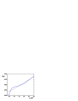
Figure 6: The integral, Eq. (24), versus the upper integration limit, $s_{0}$, for the $V$ spectral density. The integral of the experimental data corresponds to solid line and the pQCD prediction (25) is given by the dashed line.

The vector Adler function (16) obtained from matching the low momenta experimental data and high momenta pQCD asymptotics by using the spectral density (22) is shown in Fig. 7, where we use the pQCD asymptotics (23) of the massless vector spectral function to four loops with $\Lambda_{\overline{\mathrm{MS}}}^{n_{f}=3}=372$ MeV and choose the matching parameter as $s_{0}=2.5$ GeV${}^{-1}.$ Admittedly, in the Euclidean presentation of the data the detailed resonance structure corresponding to the $\rho$ and $a_{1}$ mesons seen in the Minkowski region (Fig. 5) is smoothed out, hence the verification of the theory is not as stringent as would be directly in the Minkowski space.

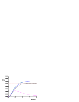
Figure 7: The Adler function from the ILM contributions: dynamical quark loop (short dashed), quark + chiral loops + vector mesons (full line) versus the ALEPH data (dashed). The dash-dotted line is the prediction of the constituent quark model (extended NJL) and the dotted line is the asymptotic freedom prediction, $1/4\pi^{2}$.

The phenomenological definition of the Adler function can be used for evaluation of the LO contribution to AMM. Below we are going to discuss the QCD model based definition of the Adler function within the instanton liquid model [29]. Next two sections we devote to the formulation of the gauged instanton liquid model [30].

4 The instanton effective quark model

Hadronic corrections to AMM are represented as the convolution integrals of some known kinematical functions times the amplitudes involving low energy quark processes. To study nonperturbative effects of these amplitudes at low momenta one can use the framework of the effective field model of QCD. In the low momenta domain the effect of the nonperturbative structure of QCD vacuum become dominant. Since invention of the QCD sum rule method based on the use of the standard OPE it is common to parameterize the nonperturbative properties of the QCD vacuum by using infinite towers of the vacuum expectation values of the quark-gluon operators. From this point of view the nonlocal properties of the QCD vacuum result from the partial resummation of the infinite series of power corrections, related to vacuum averages of quark-gluon operators with growing dimension, and may be conventionally described in terms of the nonlocal vacuum condensates [31, 32]. This reconstruction leads effectively to nonlocal modifications of the propagators and effective vertices of the quark and gluon fields at small momenta.

The adequate model describing this general picture is the instanton liquid model of QCD vacuum describing nonperturbative nonlocal interactions in terms of the effective action [29]. Spontaneous breaking of the chiral symmetry and dynamical generation of a momentum-dependent quark mass are naturally explained within the instanton liquid model. The nonsinglet and singlet $V$ and $A$ current-current correlators and the vector Adler function have been calculated in [27, 33, 34] in the framework of the effective chiral model with instanton-like nonlocal quark-quark interaction [30]. In the same model the pion structure function [35] and the pion transition form factor normalized by axial anomaly has been considered in [36] for arbitrary photon virtualities. The nonperturbative properties of the triangle diagram has been thoroughly discussed in [37, 38].

We start with the nonlocal chirally invariant action which describes the interaction of soft quark fields [30]

$$S =\int d^{4}x\ \overline{q}_{I}(x)\left[i\gamma^{\mu}D_{\mu}-m_{f}\right]q_{I}(x)+\frac{1}{2}G_{P}\int d^{4}X\int\prod_{n=1}^{4}d^{4}x_{n}f(x_{n})$$ (26)

$$\cdot\left[\overline{Q}(X-x_{1},X)\Gamma_{P}Q(X,X+x_{3})\overline{Q}(X-x_{2},X)\Gamma_{P}Q(X,X+x_{4})\right],$$

where $D_{\mu}=\partial_{\mu}-iV_{\mu}\left(x\right)-i\gamma_{5}A_{\mu}\left(x\right)$ and the spin-flavor structure of the nonlocal chirally invariant interaction of soft quarks is given by the matrix products

$$G_{P}(\Gamma_{P}\otimes\Gamma_{P}):\quad G\left(1\otimes 1+i\gamma_{5}\tau^{a}\otimes i\gamma_{5}\tau^{a}\right),\qquad G^{\prime}\left(\tau^{a}\otimes\tau^{a}+i\gamma_{5}\otimes i\gamma_{5}\right),$$ (27)

where $G$ and $G^{\prime}$ are the 4-quark couplings in the iso-triplet and iso-singlet channels, and $\tau^{a}$ are the Pauli isospin matrices. For the interaction in the form of ’t Hooft determinant one has the relation $G^{\prime}=-G$. In general due to repulsion in the singlet channel the relation $G^{\prime}<G$ is required. In Eq. (26) $\overline{q}_{I}=(\overline{u},\overline{d})$ denotes the flavor doublet field of dynamically generated quarks. The separable nonlocal kernel of the interaction determined in terms of form factors $f(x)$ is motivated by instanton model of QCD vacuum.

In order to make the nonlocal action gauge-invariant with respect to external gauge fields $V_{\mu}^{a}(x)$ and $A_{\mu}^{a}(x)$, we define in (26) the delocalized quark field, $Q(x),$ by using the Schwinger gauge phase factor

$$Q(x,y)=P\exp\left\{i\int_{x}^{y}dz_{\mu}\left[V_{\mu}^{a}(z)+\gamma_{5}A_{\mu}^{a}(z)\right]T^{a}\right\}q_{I}(y),$$

$$\overline{Q}(x,y)=Q^{\dagger}(x,y)\gamma^{0},$$ (28)

where $P$ is the operator of ordering along the integration path, with $y$ denoting the position of the quark and $x$ being an arbitrary reference point. The conserved vector and axial-vector currents have been derived earlier in [30, 27, 34].

The dressed quark propagator, $S(p)$, is defined as

$$S^{-1}(p)=i\widehat{p}-M(p^{2}),$$ (29)

with the momentum-dependent quark mass found as the solution of the gap equation

$$M(p^{2})=m_{f}+4G_{P}N_{f}N_{c}f^{2}(p^{2})\int\frac{d^{4}k}{\left(2\pi\right)^{4}}f^{2}(k^{2})\frac{M(k^{2})}{k^{2}+M^{2}(k^{2})}.$$ (30)

The formal solution is expressed as [39]

$$M(p^{2})=m_{f}+(M_{q}-m_{f})f^{2}(p^{2}),$$ (31)

with constant $M_{q}\equiv M(0)$ determined dynamically from Eq. (30) and the momentum dependent $f(p)$ is the normalized four-dimensional Fourier transform of $f(x)$ given in the coordinate representation.

The nonlocal function $f(p)$ describes the momentum distribution of quarks in the nonperturbative vacuum. Given nonlocality $f(p)$ the light quark condensate in the chiral limit, $M(p)=M_{q}f^{2}(p)$, is expressed as

$$\left\langle 0\left|\overline{q}q\right|0\right\rangle=-N_{c}\int\frac{d^{4}p}{4\pi^{4}}\frac{M(p^{2})}{p^{2}+M^{2}(p^{2})}.$$ (32)

Its $n$-moment is proportional to the vacuum expectation value of the quark condensate with the covariant with respect to gluon field derivative squared $D^{2}$ to the $n$th power

$$\left\langle 0\left|\overline{q}D^{2n}q\right|0\right\rangle=-N_{c}\int\frac{d^{4}p}{4\pi^{4}}p^{2n}\frac{M(p^{2})}{p^{2}+M^{2}(p^{2})}.$$ (33)

The $n$th moment of the quark condensate appears as a coefficient of Taylor expansion of the nonlocal quark condensate defined as [31]

$$C(x)=\left\langle 0\left|\overline{q}\left(0\right)P\exp\left[i\int_{0}^{x}A_{\mu}\left(z\right)dz_{\mu}\right]q\left(x\right)\right|0\right\rangle$$ (34)

with gluon Schwinger phase factor inserted for gauge invariance and the integral is over the straight line path. Smoothness of $C(x)$ near $x^{2}=0$ leads to existence of the quark condensate moments in the l.h.s. of (33) for any $n$. In order to make the integral in the r.h.s. of (33) convergent the nonlocal function $f(p)$ for large arguments must decrease faster than any inverse power of $p^{2}$, e.g., like some exponential

$$f\left(p\right)\sim\exp\left(-\mathrm{const\cdot}p^{\alpha}\right),~{}\alpha>0\quad\mathrm{as\quad}p^{2}\rightarrow\infty.$$ (35)

Note, that the operators entering the matrix elements in (33) and (34) are constructed from the QCD quark and gluon fields. The r.h.s. of (33) is the value of the matrix elements of QCD defined operators calculated within the effective instanton model with dynamical quark fields. Within the instanton model the zero mode function $f(p)$ depends on the gauge. It is implied [32, 35] that the r.h.s. of (33) corresponds to calculations in the axial gauge for the quark effective field. It is selected among other gauges because in this gauge the covariant derivatives become ordinary ones: $D\rightarrow\partial,$ and the exponential in (34) with straight line path is reduced to unit. In particular it means that one uses the quark zero modes in the instanton field given in the axial gauge when define the gauge dependent dynamical quark mass. The axial gauge at large momenta has exponentially decreasing behavior and all moments of the quark condensate exist. In principle, to calculate the gauge invariant matrix element corresponding to the of l.h.s. of (33) it is possible to use the expression for the dynamical mass given in any gauge, but in that case the factor $p^{2n}$ will be modified by more complicated weight function providing invariance of the answer.

Furthermore, the large distance asymptotics of the instanton solution is also modified by screening effects due to interaction of instanton field with surrounding physical vacuum [32, 40]. To take into account these effects and make numerics simpler we shell use for the nonlocal function the Gaussian form

$$f(p)=\exp\left(-p^{2}/\Lambda^{2}\right),$$ (36)

where the parameter $\Lambda$ characterizes the nonlocality size of gluon vacuum fluctuations and it is proportional to the inverse average size of instanton in the QCD vacuum.

The important property of the dynamical mass (30) is that at low virtualities its value is close to the constituent mass, while at large virtualities it goes to the current mass value. As we will see below this property is crucial in obtaining the anomaly at large momentum transfer. The instanton liquid model can be viewed as an approximation of large-$N_{c}$ QCD where the only new interaction terms, retained after integration of the high frequency modes of the quark and gluon fields down to a nonlocality scale $\Lambda$ at which spontaneous chiral symmetry breaking occurs, are those which can be cast in the form of four-fermion operators (26). The parameters of the model are then the nonlocality scale $\Lambda$ and the four-fermion coupling constant $G_{P}$.

5 Conserved vector and axial-vector currents

The quark-antiquark scattering matrix (Fig. 8) in pseudoscalar channel is found from the Bethe-Salpeter equation as

$$\widehat{T}_{P}(q^{2})=\frac{G_{P}}{1-G_{P}J_{PP}(q^{2})},$$ (37)

with the polarization operator being

$$J_{PP}(q^{2})=\int\frac{d^{4}k}{\left(2\pi\right)^{4}}f^{2}\left(k\right)f^{2}\left(k+q\right)Tr\left[S(k)\gamma_{5}S\left(k+q\right)\gamma_{5}\right].$$ (38)

Figure 8: Diagrammatic representation of the Bethe-Salpeter equation for the quark-quark scattering matrix, $T$, with nonlocal instanton kernel, $I$.

The position of pion state is determined as the pole of the scattering matrix

$$\left.\det(1-G_{P}J_{PP}(q^{2}))\right|_{q^{2}=-m_{\pi}^{2}}=0.$$ (39)

The quark-pion vertex found from the residue of the scattering matrix is $\left(k^{\prime}=k+q\right)$

$$\Gamma_{\pi}^{a}\left(k,k^{\prime}\right)=g_{\pi qq}i\gamma_{5}f(k)f(k^{\prime})\tau^{a}\quad$$ (40)

with the quark-pion coupling found from

$$g_{\pi q}^{-2}=-\left.\frac{dJ_{PP}\left(q^{2}\right)}{dq^{2}}\right|_{q^{2}=-m_{\pi}^{2}},$$ (41)

where $m_{\mathrm{\pi}}$ is physical mass of the $\pi$-meson. The quark-pion coupling, $g_{\pi q}$, and the pion decay constant, $f_{\pi}$, are connected by the Goldberger-Treiman relation, $g_{\pi}=M_{q}/f_{\pi},$ which is verified to be valid in the nonlocal model [39], as requested by the chiral symmetry.

The vector vertex following from the model (26) is (Fig. 9a)

$$\Gamma_{\mu}(k,k^{\prime})=\gamma_{\mu}+(k+k^{\prime})_{\mu}M^{(1)}(k,k^{\prime}),$$ (42)

where $M^{(1)}(k,k^{\prime})$ is the finite-difference derivative of the dynamical quark mass (see below (57)), $q$ is the momentum corresponding to the current, and $k$ $(k^{\prime})$ is the incoming (outgoing) momentum of the quark, $k^{\prime}=k+q$.

Figure 9: Diagrammatic representation of the bare (a) and full (b) quark-current vertices. Diagram (c) shows separation of local (fat dot) and nonlocal parts of the full vertex.

The full axial vertex corresponding to the conserved axial-vector current is obtained after resummation of quark-loop chain that results in appearance of term proportional to the pion propagator [30] (Fig. 9b)

$$\Gamma_{\mu}^{5}(k,k^{\prime}) =\gamma_{\mu}\gamma_{5}+2\gamma_{5}\frac{q_{\mu}}{q^{2}}f(k)f(k^{\prime})\left[J_{AP}\left(0\right)-\frac{m_{f}G_{P}J_{P}\left(q^{2}\right)}{1-G_{P}J_{PP}\left(q^{2}\right)}\right]$$

$$+(k+k^{\prime})_{\mu}J_{AP}\left(0\right)\frac{\left(f(k^{\prime})-f\left(k\right)\right)^{2}}{k^{\prime 2}-k^{2}},$$ (43)

where we have introduced the notations

$$J_{P}(q^{2})=\int\frac{d^{4}k}{\left(2\pi\right)^{4}}f\left(k\right)f\left(k+q\right)Tr\left[S(k)\gamma_{5}S\left(k+q\right)\gamma_{5}\right].$$ (44)

$$J_{AP}(q^{2})=4N_{c}N_{f}\int\frac{d^{4}l}{\left(2\pi\right)^{4}}\frac{M\left(l\right)}{D\left(l\right)}\sqrt{M\left(l+q\right)M\left(l\right)}.$$ (45)

The axial-vector vertex has a pole at

$$q^{2}=-m_{\pi}^{2}=m_{c}\left\langle\overline{q}q\right\rangle/f_{\pi}^{2}$$

where the Goldberger-Treiman relation and definition of the quark condensate have been used. The pole is related to the denominator $1-G_{P}J_{PP}\left(q^{2}\right)$ in Eq. (43), while $q^{2}$ in denominator is compensated by zero from square brackets in the limit $q^{2}\rightarrow 0.$ This compensation follows from expansion of $J(q^{2})$ functions near zero

$$J_{PP}(q^{2}) =G_{P}^{-1}+m_{c}\left\langle\overline{q}q\right\rangle M_{q}^{-2}-q^{2}g_{\pi q}^{-2}+O\left(q^{4}\right),\qquad$$ (46)

$$J_{AP}(q^{2}=0) =M_{q},\qquad J_{P}(q^{2}=0)=\left\langle\overline{q}q\right\rangle M_{q}^{-1}.$$ (47)

In the chiral limit $m_{f}=0$ the second structure in square brackets in Eq. (43) disappears and the pole moves to zero.

Within the chiral quark model [30] based on the non-local structure of instanton vacuum [32] the full singlet axial-vector vertex including local and nonlocal pieces is given by (in chiral limit) [27]

$$\Gamma_{\mu}^{5\left(0\right)}(k,q,k^{\prime}=k+q) =\gamma_{\mu}\gamma_{5}+\gamma_{5}(k+k^{\prime})_{\mu}M_{q}\frac{\left(f\left(k^{\prime}\right)-f\left(k\right)\right)^{2}}{k^{\prime 2}-k^{2}}+$$ (48)

$$+\gamma_{5}\frac{q_{\mu}}{q^{2}}2M_{q}f\left(k^{\prime}\right)f\left(k\right)\frac{G^{\prime}}{G}\frac{1-GJ_{PP}(q^{2})}{1-G^{\prime}J_{PP}(q^{2})}.$$

The singlet current (48) does not contain massless pole due to presence of the $U_{A}\left(1\right)$ anomaly. Indeed, as $q^{2}\rightarrow 0$ there is compensation between denominator and numerator in (48)

$$\frac{1-GJ_{PP}(q^{2})}{-q^{2}}=G\frac{f_{\pi}^{2}}{M_{q}^{2}}\qquad\mathrm{as}\quad q^{2}\rightarrow 0,$$ (49)

where $f_{\pi}$ is the pion weak decay constant. In cancellation of the massless pole the gap equation is used. Instead, the singlet current develops a pole at the $\eta^{\prime}-$ meson mass

$$1-G^{\prime}J_{PP}(q^{2}=-m_{\eta^{\prime}}^{2})=0,$$ (50)

thus solving the $U_{A}(1)$ problem. Let us also remind that in the instanton chiral quark model the connection between the soft gluon and effective quark degrees of freedom is fixed by the gap equation. In particular, it means that the four-quark couplings $G(G^{\prime})$ are proportional to the gluon condensate.

The parameters of the model are fixed in a way typical for effective low-energy quark models. One usually fits the pion decay constant, $f_{\pi}$, to its experimental value, which in the chiral limit reduces to $86$ MeV [41]. In the instanton model the constant, $f_{\pi}$, is expressed as

$$f_{\pi}^{2}=\frac{N_{c}}{4\pi^{2}}\int\limits_{0}^{\infty}du\ u\frac{M^{2}(u)-uM(u)M^{\prime}(u)+u^{2}M^{\prime}(u)^{2}}{D^{2}\left(u\right)},$$ (51)

where here and below $u=k^{2},$ primes mean derivatives with respect to $u$: $M^{\prime}(u)=dM(u)/du$, etc., and

$$D\left(k^{2}\right)=k^{2}+M^{2}(k).$$ (52)

One gets the values of the model parameters [34]

$$M_{q}=0.24~{}\mathrm{GeV,}\qquad\Lambda_{P}=1.11~{}\mathrm{GeV,\quad}G_{P}=27.4~{}\mathrm{GeV}^{-2}.$$ (53)

The coupling $G^{\prime}$ is fixed by fitting the meson spectrum. Approximately one has $G^{\prime}\approx 0.1~{}G$ [39].

6 Adler function within ILM.

Our goal is to obtain the vector current-current correlator and corresponding Adler function by using the effective instanton-like model (26) and then to estimate the leading order hadron vacuum polarization correction to muon anomalous magnetic moment $a_{\mu}$. In ILM in the chiral limit the (axial-)vector correlators have transverse character  [27]

$$\Pi_{\mu\nu}^{J}\left(Q^{2}\right)=\left(g_{\mu\nu}-\frac{q^{\mu}q^{\nu}}{q^{2}}\right)\Pi_{J}^{\mathrm{ILM}}\left(Q^{2}\right),$$ (54)

where the polarization functions are given by the sum of the dynamical quark loop, the intermediate (axial-)vector mesons and the higher order mesonic loops contributions (see Fig. 10)

$$\Pi_{J}^{\mathrm{ILM}}\left(Q^{2}\right)=\Pi_{J}^{Q\mathrm{Loop}}\left(Q^{2}\right)+\Pi_{J}^{\mathrm{mesons}}\left(Q^{2}\right)+\Pi_{J}^{\chi\mathrm{Loop}}\left(Q^{2}\right).$$ (55)

Figure 10: Schematic representation of the vector polarization function (55).

The spectral representation of the polarization function consists of zero width (axial-)vector resonances $\left(\Pi_{J}^{\mathrm{mesons}}\left(Q^{2}\right)\right)$ and two-meson states $\left(\Pi_{J}^{\chi\mathrm{Loop}}\left(Q^{2}\right)\right).$ The dynamical quark loop under condition of analytical confinement has no singularities in physical space of momenta.

The dominant contribution to the vector current correlator at space-like momentum transfer is given by the dynamical quark loop which was found in [27] with the result

$$\Pi_{V}^{Q\mathrm{Loop}}\left(Q^{2}\right) =\frac{4N_{c}}{Q^{2}}\int\frac{d^{4}k}{\left(2\pi\right)^{4}}\frac{1}{D_{+}D_{-}}\left\{M_{+}M_{-}+\left[k_{+}k_{-}-\frac{2}{3}k_{\perp}^{2}\right]_{ren}\right.$$ (56)

$$+\left.\frac{4}{3}k_{\perp}^{2}\left[\left(M^{\left(1\right)}\left(k_{+},k_{-}\right)\right)^{2}\left(k_{+}k_{-}-M_{+}M_{-}\right)-\left(M^{2}\left(k_{+},k_{-}\right)\right)^{\left(1\right)}\right]\right\}+$$

$$+\frac{8N_{c}}{Q^{2}}\int\frac{d^{4}k}{\left(2\pi\right)^{4}}\frac{M\left(k\right)}{D\left(k\right)}\left[M^{\prime}\left(k\right)-\frac{4}{3}k_{\perp}^{2}M^{\left(2\right)}\left(k,k+Q,k\right)\right],$$

where the notations

$$k_{\pm}=k\pm Q/2,\qquad k_{\perp}^{2}=k_{+}k_{-}-\frac{\left(k_{+}q\right)\left(k_{-}q\right)}{q^{2}},$$

$$M_{\pm}=M(k_{\pm}),\ \ \ \ \ D_{\pm}=D(k_{\pm}),$$

are used. We also introduce the finite-difference derivatives defined for an arbitrary function $F\left(k\right)$ as

$$F^{(1)}(k,k^{\prime})=\frac{F(k^{\prime})-F(k)}{k^{\prime 2}-k^{2}},\qquad F^{(2)}\left(k,k^{\prime},k^{\prime\prime}\right)=\frac{F^{(1)}(k,k^{\prime\prime})-F^{(1)}(k,k^{\prime})}{k^{\prime\prime 2}-k^{\prime 2}}.$$ (57)

In (56) the first integral represents the contribution of the dispersive diagrams and the second integral corresponds to the contact diagrams (see Fig. 11 and ref. [27] for details). The expression for $\Pi_{V}^{Q\mathrm{Loop}}\left(Q^{2}\right)$ is formally divergent and needs proper regularization and renormalization procedures which are symbolically noted by $\left[..\right]_{ren}$ for the divergent term. At the same time the corresponding Adler function is well defined and finite.

Figure 11: The dynamical quark-loop contribution is the sum of dispersive and contact terms. In the dispersive diagram $\widetilde{\Gamma}$ is the bare vertex and $\Gamma$ is the total one.

Also we have checked that there is no pole in the vector correlator as $Q^{2}\rightarrow 0$, which simply means that photon remains massless with inclusion of strong interaction. In the limiting cases the Adler function derived from Eq. (56) in accordance with the first equality of Eq. (16) satisfies general requirements of QCD (see leading terms in (18), (19), and (21))

$$A_{V}^{\mathrm{ILM}}\left(Q^{2}\rightarrow 0\right)=\mathcal{O}\left(Q^{2}\right),\qquad A_{V}^{\mathrm{ILM}}\left(Q^{2}\rightarrow\infty\right)=\frac{N_{c}}{12\pi^{2}}+\frac{O_{2}^{V}}{Q^{2}}+\mathcal{O}\left(Q^{-4}\right).$$ (58)

The leading high $Q^{2}$ asymptotics comes from the $\left[k_{+}k_{-}-\frac{2}{3}k_{\perp}^{2}\right]_{\mathrm{ren}}$ term in (56), while the subleading asymptotics is driven by ”tachionic” term with coefficient [27]

$$O_{2}^{V}=-\frac{N_{c}}{2\pi^{2}}\int_{0}^{\infty}du\frac{uM\left(u\right)M^{\prime}\left(u\right)}{D\left(u\right)}.$$ (59)

It is possible to integrate Eq. (59) in the dilute liquid approximation, $u>>M^{2}(u)$,

$$O_{2}^{V}\approx\frac{N_{c}}{4\pi^{2}}M_{q}^{2}\approx 4.7\cdot 10^{-3}\quad\mathrm{GeV}^{2},$$ (60)

which is close to exact result [27] and phenomenological estimate from [26].

In the extended by vector interaction model (26) one gets the corrections due to the inclusion of $\rho$ and $\omega$ mesons which appear as a result of quark-antiquark rescattering in these channels

$$\Pi_{V}^{\mathrm{mesons}}\left(Q^{2}\right)=\frac{1}{2Q^{2}}\frac{G_{V}B_{V}^{2}\left(Q^{2}\right)}{1-G_{V}J_{V}^{T}\left(Q^{2}\right)},$$ (61)

where $B_{V}\left(q^{2}\right)$ is the vector meson contribution to quark-photon transition form factor

$$B_{V}\left(Q^{2}\right) =8N_{c}i\int\frac{d^{4}k}{\left(2\pi\right)^{4}}\frac{f_{+}^{V}f_{-}^{V}}{D_{+}D_{-}}\left[M_{+}M_{-}-k_{+}k_{-}+\right.$$ (62)

$$\left.+\frac{2}{3}k_{\perp}^{2}\left(1-M^{2(1)}\left(k_{+},k_{-}\right)\right)-\frac{4}{3}k_{\perp}^{2}\frac{f_{-}f^{(1)}(k_{-},k_{+})}{D_{-}}\right],$$

and $J_{V}^{T}\left(q^{2}\right)$ is the vector meson polarization function defined in (38) with $\Gamma_{\mu}^{T}=\left(g_{\mu\nu}-q_{\mu}q_{\nu}/q^{2}\right)\gamma_{\nu}$. As a consequence of the Ward-Takahashi identity one has $B_{V}\left(0\right)=0$ as it should be.

To estimate the $\pi^{+}\pi^{-}$ and $K^{+}K^{-}$ vacuum polarization insertions (chiral loops corrections) one may use the effective meson vertices generated by the Lagrangian

$$-ie\ A_{\mu}\left(\pi^{+}\overleftrightarrow{\partial}_{\mu}\pi^{-}+K^{+}\overleftrightarrow{\partial}_{\mu}K^{-}\right)\ .$$ (63)

By using the spectral density calculated from this interaction:

$$\rho_{V}^{\chi loop}\left(t\right)={\frac{1}{12}}\left(1-{\frac{4m_{\pi}^{2}}{t}}\right)^{3/2}\Theta(t-4m_{\pi}^{2})+\left(\pi\rightarrow K\ \right),$$ (64)

one finds the contribution to the Adler function as

$$D_{V}^{\chi\mathrm{Loop}}\left(Q^{2}\right)=\frac{1}{48\pi^{2}}\left[a\left(\frac{Q^{2}}{4m_{\pi}^{2}}\right)+a\left(\frac{Q^{2}}{4m_{K}^{2}}\right)\right],$$ (65)

where

$$a\left(t\right)=\frac{1}{t}\left\{3+t-\frac{3}{2}\sqrt{\frac{t+1}{t}}\left[\operatorname{arctanh}\left(\frac{1+2t}{2\sqrt{t\left(t+1\right)}}\right)+i\frac{\pi}{2}\right]\right\}.$$ (66)

The estimate (65) of the chiral loop corrections corresponds to the point-like mesons which becomes unreliable at large $t,$ where the meson form factors has to be taken into account. This contribution corresponds to the lowest order, $O(p^{4})$, calculations in chiral perturbation theory ($\chi$PT), is non-leading in the formal $1/N_{c}$-expansion and provides numerically small addition. The higher-loop effects become important at higher momenta.

The resulting Adler function in ILM is given by the sum of above contributions

$$D_{V}\left(Q^{2}\right)=D_{V}^{Q\mathrm{Loop}}\left(Q^{2}\right)+D_{V}^{\mathrm{mesons}}\left(Q^{2}\right)+D_{V}^{\chi\mathrm{Loop}}\left(Q^{2}\right).$$ (67)

By using set of parameters found in ILM, , the Adler function in the vector channel (67) is presented in Fig. 7 and the model estimate for the hadronic vacuum polarization to $a_{\mu}$ given by (17) is

$$a_{\mu}^{\mathrm{hvp}~{}\left(1\right);\mathrm{ILM}}=623\left(40\right)\cdot 10^{-10}\ ,$$ (68)

where the various contributions to $a_{\mu}^{\mathrm{hvp}~{}\left(1\right);\mathrm{ILM}}$ are

$$a_{\mu}^{\mathrm{hvp}~{}\left(1\right);\mathrm{Qloop}}=533\cdot 10^{-10},\quad a_{\mu}^{\mathrm{hvp}~{}\left(1\right);\mathrm{Vmesons}}=13\cdot 10^{-10},\quad a_{\mu}^{\mathrm{hvp}~{}\left(1\right);\mathrm{\chi Loop}}=77\cdot 10^{-10}$$ (69)

and the error in (68) is due to incomplete knowledge of the higher order effects in nonchiral corrections. One may conclude, that the agreement of the instanton model estimate with the phenomenological determinations in Table 1 is rather good, but model approach unlikely reaches the required by experiment accuracy. Nevertheless, for the higher order hadronic corrections we are able essentially reduce the theoretical error by using rather sophisticated effective quark models. The realistic model calculations are a crucial issue in consideration of the NLO hadronic contributions. Reproducing the phenomenological determination of $a_{\mu}^{\mathrm{hvp}~{}\left(1\right)}$, it becomes possible to make reliable estimates of $\Delta a_{\mu}^{\mathrm{EW}}$ and $a_{\mu}^{\mathrm{h.~{}L\times L}}.$

With the same model parameters one also gets the estimate for the $\alpha^{2}$ hadronic contribution to the $\tau$-lepton anomalous magnetic moments

$$a_{\tau}^{\mathrm{hvp}~{}\left(1\right);\mathrm{ILM}}=3.1\left(0.2\right)\cdot 10^{-6}\ ,$$ (70)

which is in agreement with phenomenological determination

$$a_{\tau}^{\mathrm{hvp}~{}\left(1\right);\mathrm{exp}}=\left\{\begin{array}[c]{c}3.383\left(0.111\right)\cdot 10^{-6},\qquad\cite[cite]{[\@@bibref{}{Jegerlehner96}{}{}]},\\ 3.536\left(0.038\right)\cdot 10^{-6},\qquad\cite[cite]{[\@@bibref{}{Narison01}{}{}]},\end{array}\right.\$$

and prediction of the gauged nonlocal quark model [44]

$$a_{\tau}^{\mathrm{hvp}~{}\left(1\right);G\mathrm{NQM}}=3.2\left(0.1\right)\cdot 10^{-6}.$$

Thus, we conclude that the LO hadronic corrections obtained within the ILM are in reasonable agreement with the latest precise phenomenological numbers. Next, we are going to use the ILM in order to estimate a subset of $\alpha^{3}$ hadronic contributions to the muon anomalous magnetic moment, $a_{\mu}^{\mathrm{hvp}}$

7 $VA\widetilde{V}$ correlator and NLO corrections to $a_{\mu}$

Since discovery of anomalous properties [45, 46] of the triangle diagram with incoming two vector and one axial-vector currents [47] many new interesting results have been gained. Recently the interest to triangle diagram has been renewed due to the problem of accurate calculation of higher order hadronic contributions to muon anomalous magnetic moment via the light-by-light scattering process (Fig. 12), $a_{\mu}^{\mathrm{h.~{}L\times L}}$, that cannot be expressed as a convolution of experimentally accessible observables and need to be estimated from theory.

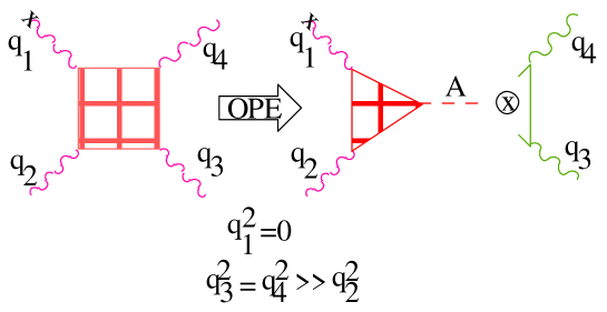
Figure 12: OPE presentation of the light-by-light scattering as the triangle amplitude times the coefficient function

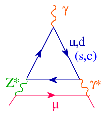
Figure 13: Effective $Z^{\ast}\gamma\gamma^{\ast}$ coupling induced by a fermion triangle contributing to $a_{\mu}^{\mathrm{EW}}$

The light-by-light scattering amplitude with one photon real and another photon has the momentum much smaller than the other two, can be analyzed using operator product expansion (OPE). In this special kinematics the amplitude is factorized into the amplitude depending on the largest photon momenta and the triangle amplitude involving the axial current $A$ and two electromagnetic currents (one soft $\widetilde{V}$ and one virtual $V$). The very similar kinematics for the triangle amplitude with quark and lepton internal lines also defines a subset of the two-loop contributions to $a_{\mu}^{\mathrm{EW}}$ via the $Z^{\ast}\gamma\gamma^{\ast}$ effective coupling (Fig. 13)

The corresponding triangle amplitude, which can be viewed as a mixing between the axial and vector currents in the external electromagnetic field, were considered recently in [20, 37, 38, 49]. This amplitude can be written as a correlator of the axial current $j_{\lambda}^{5}$ and two vector currents $j_{\nu}$ and $\tilde{j}_{\mu}$

$$\widetilde{T}_{\mu\nu\lambda}=-\int\mathrm{d}^{4}x\mathrm{d}^{4}y\,\mathrm{e}^{iqx-iky}\,\langle 0|\,T\{j_{\nu}(x)\,\tilde{j}_{\mu}(y)\,j_{\lambda}^{5}(0)\}|0\rangle\,,$$ (71)

where the currents are defined in (13), with the tilted current being for the soft momentum photon vertex. In the specific kinematics when one photon ($q_{2}\equiv q$) is virtual and another one ($q_{1}$) represents the external electromagnetic field and can be regarded as a real photon with the vanishingly small momentum $q_{1}$ depends only on two invariant functions, longitudinal $w_{L}$ and transversal $w_{T}$ with respect to axial current index [51],

$$\widetilde{T}_{\mu\nu\lambda}(q_{1},q)=\frac{1}{4\pi^{2}}\left[-w_{L}\left(q^{2}\right)q^{\lambda}q_{1}^{\rho}q^{\sigma}\varepsilon_{\rho\mu\sigma\nu}+\right.$$

$$\left.+w_{T}\left(q^{2}\right)\left(q^{2}q_{1}^{\rho}\varepsilon_{\rho\mu\nu\lambda}-q^{\nu}q_{1}^{\rho}q_{2}^{\sigma}\varepsilon_{\rho\mu\sigma\lambda}+q^{\lambda}q_{1}^{\rho}q_{2}^{\sigma}\varepsilon_{\rho\mu\sigma\nu}\right)\right].$$ (72)

Both structures are transversal with respect to vector current, $q^{\nu}\widetilde{T}_{\mu\nu\lambda}=0$. As for the axial current, the first structure is transversal with respect to $q^{\lambda}$ while the second is longitudinal and thus anomalous.

In the local theory the one-loop result for the invariant functions $w_{T}$ and $w_{L}$ is

$$w_{L}^{\mathrm{1-loop}}=2\,w_{T}^{\mathrm{1-loop}}=\frac{2N_{c}}{3}\int_{0}^{1}\frac{\mathrm{d}\alpha\,\alpha(1-\alpha)}{\alpha(1-\alpha)q^{2}+m_{f}^{2}}\,,$$ (73)

where the factor $N_{c}/3$ is due to color number and electric charge. In the chiral limit, $m_{f}=0$, one gets the result for space-like momenta $q$ $\left(q^{2}\geq 0\right)$

$$w_{L}\left(q^{2}\right)=2w_{T}\left(q^{2}\right)=\frac{2}{q^{2}}.$$ (74)

The appearance of the longitudinal structure is the consequence of the axial Adler-Bell-Jackiw anomaly [45, 46]. For the nonsinglet axial current $A^{\left(3\right)}$ there are no perturbative [52] and nonperturbative [55] corrections to the axial anomaly and, as consequence, the invariant function $w_{L}^{\left(3\right)}$ remains intact when interaction with gluons is taken into account. Recently, it was shown that the relation

$$w_{LT}\left(q^{2}\right)\equiv w_{L}\left(q^{2}\right)-2w_{T}\left(q^{2}\right)=0,$$ (75)

which holds in the chiral limit at the one-loop level (74), gets no perturbative corrections from gluon exchanges in the iso-singlet case [53]. Nonperturbative nonrenormalization of the nonsinglet longitudinal part follows from the ’t Hooft consistency condition [55], i.e. the exact quark-hadron duality realized as a correspondence between the infrared singularity of the quark triangle and the massless pion pole in terms of hadrons. OPE analysis indicates that at large $q$ the leading nonperturbative power corrections to $w_{T}$ can only appear starting with terms $\sim 1/q^{6}$ containing the matrix elements of the operators of dimension six [56]. Thus, the transversal part of the triangle with a soft momentum in one of the vector currents has no perturbative corrections nevertheless it is modified nonperturbatively. However, for the singlet axial current $A^{\left(0\right)}$ due to the gluonic $U_{A}\left(1\right)$ anomaly there is no massless state even in the chiral limit. Instead, the massive $\eta^{\prime}$ meson appears. So, one expects nonperturbative renormalization of the singlet anomalous amplitude $w_{L}^{\left(0\right)}$ at momenta below $\eta^{\prime}$ mass. Below we demonstrate how the anomalous structure $w_{L}^{\left(3\right)}$ is saturated within the instanton liquid model. We also calculate the transversal invariant function $w_{T}$ at arbitrary space-like $q$ and show that within the instanton model in the chiral limit at large $q^{2}$ all allowed by OPE power corrections to $w_{T}$ cancel each other and only exponentially suppressed corrections remain [37, 38]. The nonperturbative corrections to $w_{T}$ at large $q^{2}$ have exponentially decreasing behavior related to the short distance properties of the instanton nonlocality in the QCD vacuum.

The contribution of $Z^{\ast}\gamma\gamma^{\ast}$ vertex to the muon AMM $a_{\mu}^{\mathrm{EW}}$ in the unitary gauge, where the $Z$ propagator is $i\left(-g_{\mu\nu}+q_{\mu}q_{\nu}/m_{Z}^{2}\right)/\left(q^{2}-m_{Z}^{2}\right)$, can be written in terms of $w_{L,T}\left(q^{2}\right)$ as

$$\Delta a_{\mu}^{\mathrm{EW}} =2\sqrt{2}\frac{\alpha}{\pi}G_{\mu}m_{\mu}^{2}i\int\frac{d^{4}k}{\left(2\pi\right)^{4}}\frac{1}{q^{2}+2qp}\left[\frac{1}{3}\left(1+\frac{2\left(qp\right)^{2}}{q^{2}m_{\mu}^{2}}\right)\left(w_{L}-\frac{m_{Z}^{2}}{m_{Z}^{2}-q^{2}}w_{T}\right)+\right.$$

$$\left.+\frac{m_{Z}^{2}}{m_{Z}^{2}-q^{2}}w_{T}\right],$$ (76)

where $p$ is the four-momentum of the external muon, $G_{\mu}=1.16637(1)\cdot 10^{-5}$ GeV^-2 is the Fermi constant obtained from the muon lifetime, $m_{Z}=91.1875(21)$ GeV, $\alpha=1/137.036$ and for the electron neglecting its mass one has

$$w_{L}\left[e\right]=2w_{T}\left[e\right]=-\frac{2}{Q^{2}}.$$ (77)

In perturbative QCD with massless quarks the result for the first generation $\left[e,u,d\right]$ contribution is

$$\Delta a_{\mu}^{\mathrm{EW}}\left[e,u,d\right]=0,$$ (78)

due to anomaly cancellation.

8 $VA\widetilde{V}$ correlator within the instanton liquid model

Our goal is to obtain the nondiagonal correlator of vector current and nonsinglet axial-vector current in the external electromagnetic field ($VA\widetilde{V}$) by using the effective instanton-like model (26). In this model the $VA\widetilde{V}$ correlator is defined by (Fig. 14a)

$$\widetilde{T}_{\mu\nu\lambda}(q_{1},q_{2})=-2N_{c}\int\frac{d^{4}k}{\left(2\pi\right)^{4}}Tr\left[\Gamma_{\mu}\left(k+q_{1},k\right)S\left(k+q_{1}\right)\right.\cdot$$

$$\left.\cdot\Gamma_{\lambda}^{5}\left(k+q_{1},k-q_{2}\right)S\left(k-q_{2}\right)\Gamma_{\nu}\left(k,k-q_{2}\right)S\left(k\right)\right],$$ (79)

where the quark propagator, the vector and the axial-vector vertices are given by (29), (42) and (43), respectively. The structure of the vector vertices guarantees that the amplitude is transversal with respect to vector indices

$$\widetilde{T}_{\mu\nu\lambda}(q_{1},q_{2})q_{1}^{\mu}=\widetilde{T}_{\mu\nu\lambda}(q_{1},q_{2})q_{2}^{\nu}=0$$

and the Lorentz structure of the amplitude is given by (72).

It is convenient to express Eq. (79) as a sum of the contribution where all vertices are local (Fig. 14b), and the rest contribution containing nonlocal parts of the vertices (Fig. 14a). Further results in this section will concern the chiral limit.

Figure 14: Diagrammatic representation of the triangle diagram in the instanton model with dressed quark lines and full quark-current vertices (a); and part of the diagram when all vertices are local one (b).

The contributions of diagram 14b to the invariant functions at space-like momentum transfer, $q^{2}\equiv q_{2}^{2}$, are given by

$$w_{L}^{(loc)}\left(q^{2}\right)=\frac{4N_{c}}{9q^{2}}\int\frac{d^{4}k}{\pi^{2}}\frac{1}{D_{+}^{2}D_{-}}\left[k^{2}-4\frac{\left(kq\right)^{2}}{q^{2}}+3\left(kq\right)\right],$$ (80)

$$w_{LT}^{\left(loc\right)}\left(q^{2}\right)=0,$$ (81)

where we also consider the combination of invariant functions $w_{LT}$, (75), which show up nonperturbative dynamics. The notations used here and below are

$$k_{+}=k,\qquad k_{-}=k-q,\qquad k_{\perp}^{2}=k_{+}k_{-}-\frac{\left(k_{+}q\right)\left(k_{-}q\right)}{q^{2}},$$

$$D_{\pm}=D(k_{\pm}^{2}),\qquad M_{\pm}=M(k_{\pm}^{2}),\ \ \ \ f_{\pm}=f(k_{\pm}^{2}).\ \ \ \$$ (82)

At large $q^{2}$ one has an expansion

$$w_{L}^{(loc)}\left(q^{2}\rightarrow\infty\right)=\frac{2N_{c}}{3}\left(\frac{1}{q^{2}}+O\left(q^{-4}\right)\right)$$ (83)

It is clear that the contribution (80) saturate the anomaly at large $q^{2}$. The reason is that the leading asymptotics of (80) is given by the configuration where the large momentum is passing through all quark lines. Then the dynamical quark mass $M(k)$ reduces to zero and the asymptotic limit of triangle diagram with dynamical quarks and local vertices coincides with the standard triangle amplitude with massless quarks and, thus, it is independent of the model.

The contribution to the form factors when the nonlocal parts of the vector and axial-vector vertices are taken into account is given by

$$w_{L}^{\left(nonloc\right)}\left(q^{2}\right) =\frac{4N_{c}}{3q^{2}}\int\frac{d^{4}k}{\pi^{2}}\frac{1}{D_{+}^{2}D_{-}}\left\{M_{+}\left[M_{+}-\frac{4}{3}M_{+}^{\prime}k_{\perp}^{2}\right]-\right.$$

$$\left.-M^{2(1)}(k_{+},k_{-})\left(2\frac{\left(kq\right)^{2}}{q^{2}}-\left(kq\right)\right)\right\}.$$ (84)

Summing analytically the local (80) and nonlocal (84) parts provides us with the result required by the axial anomaly [37]

$$w_{L}(q^{2})=\frac{2N_{c}}{3}\frac{1}{q^{2}}.$$ (85)

Fig. 17 illustrates how different contributions saturate the anomaly. Note, that at zero virtuality the saturation of anomaly follows from anomalous diagram of pion decay in two photons. This part is due to the triangle diagram involving nonlocal part of the axial vertex and local parts of the photon vertices. The result (85) is in agreement with the statement about absence of nonperturbative corrections to longitudinal invariant function following from the ’t Hooft duality arguments.

For $w_{LT}(q^{2})$ a number of cancellations takes place and the final result is quite simple [37]

$$w_{LT}\left(q^{2}\right)=\frac{4N_{c}}{3q^{2}}\int\frac{d^{4}k}{\pi^{2}}\cdot$$

$$\cdot\frac{\sqrt{M_{-}}}{D_{+}^{2}D_{-}}\left\{\sqrt{M_{-}}\left[M_{+}-\frac{2}{3}M_{+}^{\prime}\left(k^{2}+2\frac{\left(kq\right)^{2}}{q^{2}}\right)\right]-\frac{4}{3}k_{\perp}^{2}\cdot\right.$$

$$\left.\cdot\left[\sqrt{M_{+}}M^{(1)}(k_{+},k_{-})-2\left(kq\right)M_{+}^{\prime}\sqrt{M}^{\left(1\right)}(k_{+},k_{-})\right]\right\}.$$ (86)

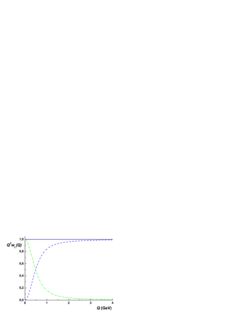
Figure 15: Normalized $w_{L}$ invariant function constrained by ABJ anomaly from triangle diagram Fig. 14a (solid line) and different contributions to it: from local part, Fig. 14b, (dashed line), and from the nonlocal part (dash-dotted line).

The behavior of $w_{LT}(q^{2})$ is presented in Fig. 17. In the above expression the integrand is proportional to the product of nonlocal form factors $f\left(k_{+}^{2}\right)f\left(k_{-}^{2}\right)$ depending on quark momenta passing through different quark lines. Then, it becomes evident that the large $q^{2}$ asymptotics of the integral is governed by the asymptotics of the nonlocal form factor $f\left(q^{2}\right)$ which is exponentially suppressed (35). Thus, within the instanton model the distinction between longitudinal and transversal parts is exponentially suppressed at large $q^{2}$ and all allowed by OPE power corrections are canceled each other. The instanton liquid model indicates that it may be possible that due to the anomaly the relation (75) is violated at large $q^{2}$ only exponentially.

The calculations of the singlet $VA\widetilde{V}$ correlator results in the following modification of the nonsinglet amplitudes [38]

$$w_{L}^{\left(0\right)}(q^{2}) =\frac{5}{3}w_{L}^{\left(3\right)}\left(q^{2}\right)+\Delta w^{\left(0\right)}\left(q^{2}\right),$$ (87)

$$w_{LT}^{\left(0\right)}(q^{2}) =\frac{5}{3}w_{LT}^{\left(3\right)}\left(q^{2}\right)+\Delta w^{\left(0\right)}\left(q^{2}\right),$$ (88)

where

$$\Delta w^{\left(0\right)}\left(q^{2}\right) =-\frac{5N_{c}}{9q^{2}}\frac{1-G^{\prime}/G}{1-G^{\prime}J_{PP}\left(q^{2}\right)}\int\frac{d^{4}k}{\pi^{4}}\frac{\sqrt{M_{+}M_{-}}}{D_{+}^{2}D_{-}}\left[M_{+}-\frac{4}{3}M_{+}^{\prime}k_{\perp}^{2}-\right.$$ (89)

$$\left.-M^{(1)}(k_{+},k_{-})\left(\frac{4}{3}\frac{\left(kq\right)^{2}}{q^{2}}+\frac{2}{3}k^{2}-\left(kq\right)\right)\right].$$

Figure 16: Normalized $w_{L}$ invariant function in the nonsinglet case (solid line) and singlet case (dashed line).

Figure 17: Normalized $w_{LT}$ invariant function versus $Q$ predicted by the instanton model in the nonsinglet case (solid line) and singlet case (dashed line).

Fig. 17 illustrates how the singlet longitudinal amplitude $w_{L}^{\left(0\right)}$ is renormalized at low momenta by the presence of the $U_{A}\left(1\right)$ anomaly. The behavior of $w_{LT}^{\left(0\right)}(q^{2})$ is presented in Fig. 17. Precise form and even sign of $w_{LT}^{\left(0\right)}(q^{2})$ strongly depend on the ratio of couplings $G^{\prime}/G$ and has to be defined in the calculations with more realistic choice of model parameters.

By using (76) one finds numerically the result for the first generation $\left[e,u,d\right]$ contribution

$$\Delta a_{\mu}^{\mathrm{EW}}\left[e,u,d\right]=-1.48\cdot 10^{-11},$$ (90)

which has to be compared with recent numbers $-2.02\cdot 10^{-11}$ [6] obtained from simple vector dominance model and $-4\cdot 10^{-11}$ [57] calculated in the naive constituent quark model.

The preliminary estimate of the hadronic light-by-light scattering contribution within the instanton liquid model is

$$a_{\mu}^{\mathrm{h.~{}L\times L}}=10.6(1.0)\cdot 10^{-10},$$ (91)

which has to be compared with in $13.6(2.5)\cdot 10^{-10}$ [20], where the simple vector meson dominance model has been used.

9 Conclusions

We briefly discussed the current status of experimental and theoretical results on the muon anomalous magnetic moment. The biggest theoretical error is due to hadronic part of AMM. The phenomenological and model approaches considered for estimates of leading and next-to-leading order hadronic corrections to muon AMM. For the model estimates one has used the instanton liquid model of QCD vacuum. We calculated the vector Adler function and the nondiagonal correlator of the vector and axial-vector currents in the background of a soft vector field for arbitrary space-like momenta transfer and found the corrections to muon anomaly coming from the effects of hadronic vacuum polarization, $Z^{\ast}\gamma\gamma^{\ast}$ effective vertex and light-by-light scattering.

The author is grateful to Organizers of the School and in particular to Michal Praszalowicz for creating of very fruitful atmosphere at the school. The author also thanks for partial support from the Russian Foundation for Basic Research projects nos. 03-02-17291, 04-02-16445.

References

- [1] T. Kinoshita, M. Nio, Phys. Rev. D 70 (2004) 113001 and references therein.
- [2] G.W. Bennett et al. [Muon g-2 Collaboration], Phys. Rev. Lett. 92 (2004) 161802.
- [3] R.M. Carey et. al., (2004) Proposal of the BNL Experiment E969 (www.bnl.gov/henp/docs/pac0904/P969.pdf); B.L. Roberts, (2005) hep-ex/0501012.
- [4] J-PARC Letter of Intent L17, B.L. Roberts , contact person.
- [5] M.N. Achasov et.al. [SND Collaboration], arXiv:hep-ex/0506076.
- [6] A. Czarnecki, W. J. Marciano and A. Vainshtein, Phys. Rev. D 67 (2003) 073006.
- [7] C. Bouchiat and L. Michel, J. Phys. Radium, 22 121.
- [8] L. Durand, Phys. Rev., 128 (1962) 441.
- [9] R. Barate et.al. [ALEPH Collaboration], Eur. Phys. J. C 4 (1998) 409.
- [10] K. Ackerstaff et.al. [OPAL Collaboration], Eur. Phys. J. C 7 (1999) 571.
- [11] S. Anderson et.al. [CLEO Collaboration], Phys. Rev. D 61 (2000) 112002.
- [12] R.R. Akhmetshin et.al. [CMD-2 Collaboration], Phys. Lett. B 578 (2004) 285.
- [13] A. Aloisio et.al. [KLOE Collaboration], Phys. Lett. B 606 (2005) 12.
- [14] M. Davier, S. Eidelman, A. Hocker and Z. Zhang, Eur. Phys. J. C 31 (2003) 503.
- [15] S. Ghozzi, F. Jegerlehner, Phys. Lett. B 583 (2004) 222.
- [16] J.F. de Troconiz, F.J. Yndurain, Phys. Rev. D 71 (2005) 073008.
- [17] B. Krause, Phys. Lett. B 390 (1997) 392.
- [18] R. Barbieri, E. Remiddi, Nucl. Phys. B 90 (1975) 233.
- [19] Yu.M. Bystritskiy et.al., arXiv:hep-ph/0506317.
- [20] K. Melnikov, A. Vainshtein, Phys. Rev. D 70 (2004) 113006.
- [21] K. Maltman, hep-ph/0504201.
- [22] B.E. Lautrup and E. de Rafael, Nuovo Cimento, 64 A, (1969), 322.
- [23] S.G. Gorishnii, A.L. Kataev, S.A. Larin, Phys. Lett. B 259 (1991) 144; L.R. Surguladze, M.A. Samuel, Phys. Rev. Lett. 66 (1991) 560 [Erratum-ibid. 66 (1991) 2416].
- [24] K.G. Chetyrkin, Phys. Lett. B 391 (1997) 402.
- [25] M.A. Shifman, A.I. Vainshtein and V.I. Zakharov, Nucl. Phys. B 147, 448 (1979).
- [26] K.G. Chetyrkin, S. Narison, V.I. Zakharov, Nucl. Phys. B 550 (1999) 353.
- [27] A. E. Dorokhov, W. Broniowski, Eur. Phys. J. C 32 (2003) 79.
- [28] S. Peris, M. Perrottet, E. de Rafael, JHEP 9805 (1998) 011.
- [29] See for review, e.g., T. Schafer, E.V. Shuryak, Rev. Mod. Phys. 70 (1998) 323.
- [30] I. V. Anikin, A. E. Dorokhov and L. Tomio, Phys. Part. Nucl. 31 (2000) 509 [Fiz. Elem. Chast. Atom. Yadra 31 (2000) 1023].
- [31] S.V. Mikhailov, A.V. Radyushkin, Sov. J. Nucl. Phys. 49 (1989) 494 [Yad. Fiz. 49 (1988) 794]; S. V. Mikhailov and A. V. Radyushkin, Phys. Rev. D 45 (1992) 1754.
- [32] A. E. Dorokhov, S. V. Esaibegian and S. V. Mikhailov, Phys. Rev. D 56 (1997) 4062; A.E. Dorokhov, S.V. Esaibegyan, A. E. Maximov, S.V. Mikhailov, Eur. Phys. J. C 13 (2000) 331.
- [33] A. E. Dorokhov, Phys. Part. Nucl. Lett. 1 (2004) 240.
- [34] A. E. Dorokhov, Phys. Rev. D 70 (2004) 094011.
- [35] A. E. Dorokhov and L. Tomio, Phys. Rev. D 62 (2000) 014016.
- [36] A. E. Dorokhov, JETP Letters, 77 (2003) 63 [Pisma ZHETF, 77 (2003) 68]; I. V. Anikin, A. E. Dorokhov and L. Tomio, Phys. Lett. B 475 (2000) 361; I.V. Anikin, A.E. Dorokhov, A.E. Maksimov, L. Tomio, V. Vento, Nucl. Phys. A 678 (2000) 175.
- [37] A.E. Dorokhov, Eur. Phys. J. C 42 (2005) 309.
- [38] A.E. Dorokhov, JETP Letters, 82 (2005) 1 [Pisma ZHETF, 82 (2005) 3].
- [39] R.S. Plant and M. C. Birse, Nucl. Phys. A 628 (1998) 607.
- [40] A. E. Dorokhov and W. Broniowski, Phys. Rev. D 65 (2002) 094007.
- [41] J. Gasser, H. Leutwyler, Annals Phys. 158, (1984) 142.
- [42] F. Jegerlehner, Nucl. Phys. Proc. Suppl. 51C (1996) 131.
- [43] S.Narison, Phys. Lett. B 513 (2001) 53[Erratum-ibid. B 526 (2002) 414]
- [44] B. Holdom, R. Lewis and R.R. Mendel, Z. Phys. C 63 (1994) 71.
- [45] S. L. Adler, Phys. Rev. 177 (1969) 2426.
- [46] J. S. Bell and R. Jackiw, Nuovo Cim. A 60 (1969) 47.
- [47] L. Rosenberg, Phys. Rev. 129 (1963) 2786.
- [48] S. Groote, J. G. Körner, A. A. Pivovarov, Eur. Phys. J. C 24 (2002) 393.
- [49] A. Czarnecki, W. J. Marciano and A. Vainshtein, Phys. Rev. D 67 (2003) 073006.
- [50] A. Czarnecki, Acta Phys. Polon. B 33 (2002) 4373.
- [51] T. V. Kukhto, E. A. Kuraev, Z. K. Silagadze and A. Schiller, Nucl. Phys. B 371 (1992) 567.
- [52] S. L. Adler and W. A. Bardeen, Phys. Rev. 182 (1969) 1517.
- [53] A. Vainshtein, Phys. Lett. B 569 (2003) 187.
- [54] R.S. Pasechnik, O.V. Teryaev, arXiv:hep-ph/0510290.
- [55] G. ’t Hooft, in Recent Developments In Gauge Theories, Eds. G. ’t Hooft et al., (Plenum Press, New York, 1980).
- [56] M. Knecht, S. Peris, M. Perrottet and E. De Rafael, JHEP 0211 (2002) 003.
- [57] A. Czarnecki, B. Krause, W. J. Marciano, Phys. Rev. D 52 (1995) 2619.