hep-ph/0510275

TASI Lectures on Electroweak Symmetry Breaking from Extra Dimensions

Csaba Csáki, Jay Hubisz and Patrick Meade

Institute of High Energy Phenomenology,
Newman Laboratory of Elementary Particle Physics,
Cornell University, Ithaca, NY 14853

csaki,hubisz,meade@lepp.cornell.edu

This is a pedagogical introduction into the possible uses and effects of extra dimensions in electroweak (TeV scale) physics, and in particular to models of electroweak symmetry breaking via boundary conditions (“higgsless models”). It is self contained: all the aspects of extra dimensional and electroweak physics used here are reviewed, before we apply these concepts to higgsless models. In the first lecture gauge theories in an extra dimension and on an interval are discussed. In the second lecture we describe the basic structure of higgsless models, while in the third lecture we discuss fermions in extra dimensions and the inclusion of fermions into higgsless models. The final lecture is devoted to the issue of electroweak precision observables in theories beyond the standard model and its applications to extra dimensional theories and in particular the higgsless models.

1 Introduction

Theories with extra dimensions have again become very popular over the past ten years. The reason why is that it was realized that extra dimensions could actually play an active role in the physics of the TeV scales (rather than being irrelevant up to the Planck scale). The first proposal along these lines were theories with large extra dimensions [1], where one would explain the discrepancy of the weak and Planck scale via the presence of large extra dimensions diluting the strength of gravitational interactions. The second main wave of excitement was brought on by the Randall-Sundrum models [2, 3], where it was understood that the geometry of the extra dimensions could actually lead to novel approaches to the hierarchy problem or even to 4D gravity. Many of the aspects of these models have been reviewed in a previous TASI lecture [4] (and other excellent introductions to these topics include lectures at this TASI given by Graham Kribs [5] and Raman Sundrum [6], and can also be found in [7]). The aim of these lectures is to emphasize less (compared to [4]) the gravitational aspects of extra dimensional theories, but rather the use of such models for electroweak physics. Some knowledge of the material in [4] could be useful for reading these notes, however we have attempted to present a self-contained series of lectures focusing on gauge theories in extra dimensions.

In the first lecture we discuss generalities about extra dimensional gauge theories. We mostly focus on the issue of how to assign a consistent set of boundary conditions (BC’s) after proper gauge fixing. We also comment on the relation between the orbifold and the interval approaches to describing an extra dimension with a boundary. In the second lecture we apply the tools from the first lecture towards building an extra dimensional model where electroweak symmetry is broken via BC’s (rather than by a scalar higgs). Such models will be referred to as higgsless models, and will serve throughout these notes as the canonical example of applying the various concepts discussed. In order to find a (close to) realistic higgsless model we need to review the basics of the AdS/CFT correspondence for warped extra dimensions. The third lecture deals with fermions in extra dimensions. After a brief review of fermions in general we show how one generically introduces fermions into extra dimensional models and how theories with boundaries can render such models chiral. We then show how these tools can be applied to higgsless models to obtain a realistic fermion mass spectrum. Finally, we discuss the issue of how to calculate corrections to electroweak precision observables in theories beyond the standard model. We give a general effective field theory approach applicable to any model, and show how the Peskin-Takeuchi S,T,U formalism fits into it. We then show how these parameters can be generically calculated in an extra dimensional model, and evaluate it for the higgsless theory.

2 Gauge theories in an extra dimension and on an interval

In this first lecture we will be discussing the structure of a gauge theory in a single extra dimension. For now we will be assuming that there is no non-trivial gravitational background, that is the extra dimension is flat. However we still need to discuss what the geometry of the extra dimension is. There are three distinct possibilities:

• Totally infinite extra dimension like the other 3+1 dimensions

• The extra dimension is a half-line, that is infinite in one direction

• Finite extra dimension: this could either be a circle or an interval

For now we will not be dealing with the very interesting possibility of a half-infinite extra dimension, which could be phenomenologically viable in the case of localized gravity (the so-called RS2 model [3]). In most interesting cases one has to deal with a compactified extra dimension.

The first question we will be discussing in detail is how to define a field theory with an extra dimension classically. When the space is infinite, one usually requires that the fields vanish when the coordinates go to infinity, that is

$$\psi\to 0\ {\rm as}\ r\ \to\infty$$ (2.1)

However when the space is finite, one does not necessarily need to impose $\psi\to 0$ as the boundary conditions (BC’s). What will be the possible BC’s then? The two possibilities as mentioned above for the finite extra dimensions are

• circle ($\equiv$ an interval with the ends identified): in this case the boundary conditions for the fields are clear, $\Psi(2\pi R)=\Psi(0)$.

• interval ($\equiv$ the ends are not identified)

In either case, we can just start from the action principle and see what BC’s one can impose that are consistent with the action principle. As the simplest example let us first discuss the case of a single scalar field in an extra dimension [8, 9].

2.1 A scalar field on an interval

We start with a bulk action for the scalar field

$$S_{bulk}=\int d^{4}x\int_{0}^{\pi R}\left(\frac{1}{2}\partial^{M}\phi\partial_{M}\phi-V(\phi)\right)dy,$$ (2.2)

where we have assumed that the interval runs between $0$ and $\pi R$. The coordinates are labelled by $M=0,1,2,3,5$, while Greek letters $\mu,\nu,\ldots$ will denote our usual four dimensions $0,1,2,3$. We will also assume throughout these lectures that the signature of the metric is given by

$$g_{MN}=\left(\begin{array}[]{ccccc}1\\ &-1\\ &&-1\\ &&&-1\\ &&&&-1\end{array}\right)$$ (2.3)

We will for simplicity first assume that there is no term added on the boundary of the interval. Let us apply the variational principle to this theory:

$$\delta S=\int d^{4}x\int_{0}^{\pi R}\left(\partial^{M}\phi\partial_{M}\delta\phi-\frac{\partial V}{\partial\phi}\delta\phi\right)dy.$$ (2.4)

Separating out the ordinary 4D coordinates from the fifth coordinate (and integrating by parts in the ordinary 4D coordinates, where we apply the usual requirements that the fields vanish for large distances) we get

$$\delta S=\int d^{4}x\int_{0}^{\pi R}dy\left[-\partial_{\mu}\partial^{\mu}\phi\delta\phi-\frac{\partial V}{\partial\phi}\delta\phi-\partial_{y}\phi\partial_{y}\delta\phi\right]$$ (2.5)

Since we have not yet decided what boundary conditions one wants to impose we will have to keep the boundary terms when integrating by parts in the fifth coordinate $y$:

$$\delta S=\int d^{4}x\int_{0}^{\pi R}\left[-\partial_{M}\partial^{M}\phi-\frac{\partial V}{\partial\phi}\right]\delta\phi-\left[\int d^{4}x\partial_{y}\phi\delta\phi\right]_{0}^{\pi R}.$$ (2.6)

To ensure that the variational principle is obeyed, we need $\delta S=0$, but since this consists of a bulk and a boundary piece we require:

• The bulk equation of motion (EOM) $\partial_{M}\partial^{M}\phi=-\frac{\partial V}{\partial\phi}$ as usual

• The boundary variation needs to also vanish. This implies that one needs to choose the BC such that

  $$\partial_{y}\phi\delta\phi|_{bound}=0.$$ (2.7)

We will be calling a boundary condition natural, if it is obtained by letting the boundary variation of the field $\delta\phi|_{bound}$ to be arbitrary. In this case the natural BC would be $\partial_{y}\phi=0$ – a flat or Neumann BC. But at this stage this is not the only possibility: one could also satisfy (2.7) by imposing $\delta\phi|_{bound}=0$ which would follow from the $\phi|_{bound}=0$ Dirichlet BC. Thus we get two possible BC’s for a scalar field on an interval with no boundary terms:

• Neumann BC $\partial_{y}\phi|=0$

• Dirichlet BC $\phi|=0$

However, we would only like to allow the natural boundary conditions in the theory since these are the ones that will not lead to explicit (hard) symmetry breaking once more complicated fields like gauge fields are allowed. Thus in order to still allow the Dirichlet BC one needs to reinterpret that as the natural BC for a theory with additional terms in the Lagrangian added on the boundary. The simplest possibility is to add a mass term to modify the Lagrangian as

$$S=S_{bulk}-\int d^{4}x\frac{1}{2}M_{1}^{2}\phi^{2}|_{y=0}-\int d^{4}x\frac{1}{2}M_{2}^{2}\phi^{2}|_{y=\pi R}.$$ (2.8)

These will give an additional contribution to the boundary variation of the action, which will now given by:

$$\delta S_{bound}=-\int\delta\phi(\partial\phi+M_{2}^{2}\phi)|_{y=\pi R}+\int d^{4}x\delta\phi(\partial_{y}\phi-M_{1}^{2}\phi)|_{y=0}.$$ (2.9)

Thus the natural BC’s will be given by

$$\partial_{y}\phi+M_{2}^{2}\phi=0\ \ {\rm at}\ \ y=\pi R,$$

$$\partial_{y}\phi-M_{1}^{2}\phi=0\ \ {\rm at}\ \ y=0.$$ (2.10)

Clearly, for $M_{i}\to\infty$ we will recover the Dirichlet BC’s in the limit. This is the way we will always understand the Dirichlet BC’s: we will interpret them as the case with infinitely large boundary induced mass terms for the fields.

Let us now consider what happens in the case [10] when we add a kinetic term on the boundary (which we will also be calling branes throughout these lectures) for $\phi$. This is a somewhat tricky question that had many people confused for a while. For simplicity let us set the mass parameters on the branes to zero, and take as the action

$$S=S_{bulk}+\int d^{4}x\frac{1}{2M}\partial_{\mu}\phi\partial^{\mu}\phi|_{y=0}.$$ (2.11)

Note that the boundary term had to be added with a definite sign, that is we assume that the arbitrary mass parameter $M$ is positive. This is in accordance with our expectations that kinetic terms have to have positive signs if one wants to avoid ghostlike states. For simplicity we have only added a kinetic term on one of the branes, but of course we could easily repeat the following analysis for the second brane as well. The boundary variation at $y=0$ will be modified to

$$\delta S|_{0}=\int d^{4}x\delta\phi(\partial_{y}\phi-\frac{1}{M}\Box_{4}\phi)|_{y=0}.$$ (2.12)

Thus the natural BC will be given by:

$$\partial_{y}\phi=\frac{1}{M}\Box_{4}\phi.$$ (2.13)

Using the bulk equation of motion (in the presence of no bulk potential) $\Box_{5}\phi=\Box_{4}\phi-\phi^{\prime\prime}=0$ we could also write this BC as $\phi^{\prime}=\frac{1}{M}\phi^{\prime\prime}$. The final form of the BC is obtained by using the Kaluza-Klein (KK) decomposition of the field $\phi$ where one usually assumes that the 4D modes $\phi_{n}$ have the $x$ dependence $\phi_{n}(y)e^{ip_{n}\cdot x}$, where $p_{n}^{2}=m_{n}^{2}$ is the n^th KK mass eigenvalue. Using this form the BC will be given by:

$$\partial_{y}\phi=\frac{1}{M}\Box_{4}\phi=-\frac{p_{n}^{2}}{M}\phi=-\frac{m_{n}^{2}}{M}\phi.$$ (2.14)

In either form this BC is quite peculiar: it depends on the actual mass eigenvalue in the final form, or involves second derivatives in the first form. This could be dangerous, since from the theory of differential equations we know that usually BC’s that only involve first derivatives are the ones that will automatically lead to a hermitian differential operator on an interval. The usual reason is that the second derivative operator $d^{2}/dy^{2}$ is hermitian if the scalar product

$$(f,g)=\int_{0}^{\pi R}f^{*}(y)g(y)$$ (2.15)

obeys the relation

$$(f,\frac{d^{2}}{dy^{2}}g)=(\frac{d^{2}}{dy^{2}}f,g).$$ (2.16)

These two terms can be easily transformed into each other using two integrations by parts up to two boundary terms:

$$(f,\frac{d^{2}}{dy^{2}}g)=\int_{0}^{\pi R}f^{*}(y)\frac{d^{2}}{dy^{2}}g(y)=-\int_{0}^{\pi R}{f^{*}}^{\prime}(y)g^{\prime}(y)+[f^{*}(y)g^{\prime}(y)]_{0}^{\pi R}=$$

$$=\int_{0}^{\pi R}{f^{*}}^{\prime\prime}(y)g(y)+[f^{*}(y)g^{\prime}(y)]_{0}^{\pi R}-[{f^{*}}^{\prime}(y)g(y)]_{0}^{\pi R}.$$ (2.17)

Thus we can see that if the boundary condition for the functions on which we define this scalar product is of the form

$$f^{\prime}|_{0,\pi R}=\alpha f|_{0,\pi R}$$ (2.18)

then the two boundary terms will cancel each other and the operator $d^{2}/dy^{2}$ is hermitian, and the desired properties (completeness, real eigenvalues) will automatically follow. However, the boundary condition $f^{\prime\prime}=1/Mf^{\prime}$ is not of this form, and the second derivative operator is naively not hermitian. This is indeed the case, however, one can choose a different definition of the scalar product on which the above boundary condition will nevertheless ensure the hermiticity of the second derivative operator. To find what this scalar product should be, let us try to prove the orthogonality of two distinct eigenfunctions of the second derivative operator. Let $f$ and $g$ be two eigenfunctions of the second derivative operator $f^{\prime\prime}=\lambda_{f}f$ and $g^{\prime\prime}=\lambda_{g}g$, then

$$\int_{0}^{\pi R}f^{*}g^{\prime\prime}dy=\lambda_{g}\int_{0}^{\pi R}f^{*}(y)g(y)dy=\int_{0}^{\pi R}f^{*^{\prime\prime}}(y)g(y)dy+f^{*^{\prime}}g|_{0}-g^{\prime}f^{*}|_{0}.$$ (2.19)

Using the boundary condition $f^{\prime\prime}=Mf^{\prime}=\lambda_{f}f$, so $f^{\prime}=\lambda_{f}/Mf$ we find that

$$(\lambda_{f}-\lambda_{g})\left(\int_{0}^{\pi R}f(y)g(y)dy+\frac{1}{M}fg|_{0}\right)=0.$$ (2.20)

What we find is the combination that is orthogonal, which means that this is the combination that one should call the scalar product in the presence of a non-trivial boundary kinetic term. Thus the scalar product in this case should be defined by

$$(f,g)=\int_{0}^{\pi R}f(y)g(y)dy+\frac{1}{M}fg|_{0}$$ (2.21)

This definition still satisfies all the properties that a scalar product should satisfy, and with this definition the second derivative operator will now be hermitian. This is easy to check:

$$(f,g^{\prime\prime})=\int_{0}^{\pi R}fg^{\prime\prime}dy+\frac{1}{M}fg^{\prime\prime}|_{0}=-\int_{0}^{\pi R}f^{\prime}g^{\prime}dy-fg^{\prime}|_{0}+\frac{1}{M}fg|_{0}=$$

$$=\int f^{\prime\prime}gdy+f^{\prime}g|_{0}-fg^{\prime}|_{0}+\frac{1}{M}fg^{\prime\prime}|_{0}.$$ (2.22)

Due to the BC $g^{\prime\prime}=Mg^{\prime}$ the last two boundary terms cancel, and the first can be rewritten as $\frac{1}{M}f^{\prime\prime}g|_{0}$, and so the full expression really equals $(f^{\prime\prime},g)$. So we have shown that there really is no problem with a theory with brane kinetic terms added. However, one needs to be careful when using a KK decomposition: the proper scalar product needs to be used when one is trying to use the orthogonality and the completeness of the wavefunctions. For example, the completeness relation will be given by

$$\sum_{n}g_{n}(x)g_{n}(y)=\delta(x-y)-\frac{1}{M}\delta(x)\sum_{n}g_{n}(0)g_{n}(y).$$ (2.23)

2.2 Pure gauge theories on an interval: gauge fixing and BC’s

Next we will consider a pure gauge theory in an extra dimension [11, 9, 12]. A gauge field in 5D $A_{M}$ contains a 4D gauge field $A_{\mu}$ and a 4D scalar $A_{5}$. The 4D vector will contain a whole KK tower of massive gauge bosons, however as we will see below the KK tower of the $A_{5}$ will be eaten by the massive gauge fields and (except for a possible zero mode) will be non-physical. That this is what happens can be guessed from the fact that the Lagrangian contains a mixing term between the gauge fields and the scalar, reminiscent of the usual 4D Higgs mechanism. The Lagrangian is given by the usual form

$$S=\int d^{5}x(-\frac{1}{4}F_{MN}^{a}F^{MN\,a})=\int d^{5}x(-\frac{1}{4}F_{\mu\nu}^{a}F^{\mu\nu\,a}-\frac{1}{2}F_{\mu 5}^{a}F^{\mu 5\,a}),$$ (2.24)

where the field strength is given by the usual expression $F_{MN}^{a}=\partial_{M}A_{N}^{a}-\partial_{N}A_{M}^{a}+g_{5}f^{abc}A_{M}^{b}A_{N}^{c}$. $g_{5}$ is the 5D gauge coupling, which has mass dimension $-1/2$, thus the theory is non-renormalizable, so it has to be considered as a low-energy effective theory valid below a cutoff scale, that we will be calculating later on.

To determine the gauge fixing term, let us consider the mixing term between the scalar and the gauge fields:

$$\int d^{4}x\int_{0}^{\pi R}dy-\frac{1}{2}F_{\mu 5}^{a}F^{\mu 5\ a}|_{quadratic}=$$

$$\int d^{4}x\int_{0}^{\pi R}dy-\frac{1}{2}(\partial_{\mu}A_{5}^{a}-\partial_{5}A_{\mu}^{a})(\partial^{\mu}A^{5\ a}-\partial^{5}A^{\mu\ a})=$$

$$\int d^{4}x\int_{0}^{\pi R}dy-\frac{1}{2}(\partial_{\mu}A_{5}^{a}\partial^{\mu}A^{5\ a}+\partial_{5}A_{\mu}^{a}\partial^{5}A^{\mu\ a}-2\partial_{5}A_{\mu}^{a}\partial^{\mu}A^{5a}).$$ (2.25)

Thus the mixing term that needs to be cancelled is given by

$$\int_{0}^{\pi R}\partial_{5}A_{\mu}^{a}\partial^{\mu}A^{5a}.$$ (2.26)

Integrating by parts we find

$$-\int_{0}^{\pi R}\partial^{\mu}A_{\mu}^{a}\partial_{5}A_{5}^{a}+[\partial_{\mu}A^{\mu a}A_{5}^{a}]_{0}^{\pi R}.$$ (2.27)

The bulk term can be cancelled by adding a gauge fixing term of the form

$$S_{GF}=\int d^{4}x\int_{0}^{\pi R}-\frac{1}{2\xi}(\partial_{\mu}A^{\mu a}-\xi\partial_{5}A_{5}^{a})^{2}.$$ (2.28)

This term is chosen such that the $A_{5}$ independent piece agrees with the usual Lorentz gauge fixing term, and such that the cross term exactly cancels the mixing term from (2.27). Thus within $R_{\xi}$ gauge, which is what we have defined, the propagator for the 4D gauge fields will be the usual ones. Varying the full action we then obtain the bulk equations of motion and the possible BC’s. After integrating by parts we find:

$$\delta S_{bulk}=\int d^{4}x\int_{0}^{\pi R}\left[(\partial_{M}F^{M\nu a}-g_{5}f^{abc}F^{M\nu b}A_{M}^{c}+\frac{1}{\xi}\partial^{\nu}\partial^{\sigma}A_{\sigma}^{a}-\partial^{\nu}\partial_{5}A_{5}^{a})\delta A_{\nu}^{a}+\right.$$

$$\left.(\partial^{\sigma}F^{a}_{\sigma 5}-g_{5}f^{abc}F^{b}_{\sigma 5}A^{c\sigma}\partial_{5}\partial_{\sigma}A^{a\sigma}-\xi\partial_{5}^{2}A_{5}^{a})\delta A_{5}^{a}\right]$$ (2.29)

The bulk equations of motion will be that the coefficients of $\delta A_{\nu}^{a}$ and $\delta A_{5}^{a}$ in the above equation vanish. We can see, that the $A_{5}^{a}$ field has a term $\xi\partial_{5}^{2}A_{5}^{a}$ in its equation. This will imply that if the wave function is not flat (e.g. the KK mode is not massless), then the field is not physical (since in the unitary gauge $\xi\to\infty$ this field will have an infinite effective 4D mass and decouples). This shows that as mentioned above, the scalar KK tower of $A_{5}^{a}$ will be completely unphysical due to the 5D Higgs mechanism, except perhaps for a zero mode for $A_{5}^{a}$. Whether or not there is a zero mode depends on the BC for the $A_{5}$ field. We will see later how to interpret $A_{5}$ zero modes.

In order to eliminate the boundary mixing term in (2.27), we also need to add a boundary gauge fixing term with an a priori unrelated boundary gauge fixing coefficient $\xi_{bound}$:

$$-\frac{1}{2\xi_{bound}}\int d^{4}x(\partial_{\mu}A^{\mu a}\pm\xi_{bound}A_{5}^{a})^{2}|_{0,\pi R},$$ (2.30)

where the $-$ sign is for $y=0$ and the $+$ for $y=\pi R$. The boundary variations are then given by:

$$(\partial_{5}A^{\mu a}+\frac{1}{\xi_{bound}}\partial_{\nu}\partial^{\mu}A^{\nu a})\delta A_{\mu}^{a}|_{0,\pi R}+(\xi\partial_{5}A_{5}^{a}\pm\xi_{bound}A_{5}^{a})\delta A_{5}^{a}|_{0,\pi R}.$$ (2.31)

The natural boundary conditions in an arbitrary gauge $\xi,\xi_{bound}$ are given by

$$\partial_{5}A^{\mu a}+\frac{1}{\xi_{bound}}\partial_{\mu}\partial^{\mu}A^{\mu a}=0,\ \ \xi\partial_{5}A_{5}^{a}\pm\xi_{bound}A_{5}^{a}=0.$$ (2.32)

This simplifies quite a bit if we go to the unitary gauge on the boundary given by $\xi_{bound}\to\infty$. In this case we are left with the simple set of boundary conditions

$$\partial_{5}A^{\mu a}=0,\ \ A_{5}^{a}=0.$$ (2.33)

This is the boundary condition that one usually imposed for gauge fields in the absence of any boundary terms. Note, that again we could have chosen some non-natural boundary conditions, where instead of requiring that the boundary variation be arbitrary we would require the boundary variation itself (and thus some of the fields on the boundary) to be vanishing. It turns out that these boundary conditions would lead to a hard (explicit) breaking of gauge invariance, and thus we will not consider them in the following discussion any further. We will see below how these simple BC’s will be modified if one adds scalar fields on the branes.

2.3 Gauge theories with boundary scalars

Let us now consider the case when scalar fields that develop VEV’s are added on the boundary [9, 12]. For simplicity we will be considering a U(1) theory, but it can be straightforwardly generalized to more complicated groups. The localized Lagrangians for the two complex scalar fields $\Phi_{i}$ will be the usual ones for a Higgs field in 4D, and the subscripts $i=1,2$ correspond to the two boundaries:

$${\cal L}_{i}=|D_{\mu}\Phi_{i}|^{2}-\lambda_{i}(|\Phi_{i}|^{2}-\frac{1}{2}v_{i}^{2})^{2}.$$ (2.34)

These boundary terms will induce non-vanishing VEV’s and we parameterize the Higgs as usual as a physical Higgs and a Goldstone (pion):

$$\Phi_{i}=\frac{1}{\sqrt{2}}(v_{i}+h_{i})e^{i\pi_{i}/v_{i}}.$$ (2.35)

We can now expand again the action to quadratic order in the fields to find the expression

$${\cal L}_{4D}= \int_{0}^{\pi R}dy\left(-\frac{1}{4}F_{\mu\nu}^{2}+\frac{1}{2}(\partial_{\mu}A_{5})^{2}-\partial_{\mu}A_{5}\partial_{5}A^{\mu}\right)$$ (2.36)

$$+\left[\frac{1}{2}(\partial_{\mu}h_{1})^{2}-\frac{1}{2}\lambda_{1}v_{1}^{2}h_{1}^{2}+\frac{1}{2}(\partial_{\mu}\pi_{1}-v_{1}A_{\mu})^{2}\right]_{y=0}$$

$$+\left[\frac{1}{2}(\partial_{\mu}h_{2})^{2}-\frac{1}{2}\lambda_{2}v_{2}^{2}h_{2}^{2}+\frac{1}{2}(\partial_{\mu}\pi_{2}-v_{2}A_{\mu})^{2}\right]_{y=\pi R}$$

Repeating the procedure in the previous section and integrating by parts, we find that the following bulk and boundary gauge fixing terms are necessary in order to eliminate all the mixing terms between the gauge field and the scalars $A_{5},\pi_{i}$:

$${\cal L}_{GF}= -\frac{1}{2\xi}\int_{0}^{\pi R}dy(\partial_{\mu}A^{\mu}-\partial_{5}A_{5})^{2}-\left[\frac{1}{2\xi_{1}}(\partial_{\mu}A^{\mu}+\xi_{1}(v_{1}\pi_{1}-A_{5}))^{2}\right]_{y=0}$$ (2.37)

$$-\left[\frac{1}{2\xi_{2}}(\partial_{\mu}A^{\mu}+\xi_{2}(v_{2}\pi_{2}+A_{5}))^{2}\right]_{y=\pi R}$$

With this gauge fixing the gauge field will be decoupled from the rest of the fields, and its bulk action will be given by

$$\int d^{5}x\frac{1}{2}A_{\mu}\left[(\partial^{2}-\partial_{y}^{2})\eta^{\mu\nu}-(1-\frac{1}{\xi})\partial^{\mu}\partial^{\nu}\right]A_{\nu}.$$ (2.38)

The KK decomposition can then be obtained by writing the field as

$$A_{\mu}(x,y)=\epsilon_{\mu}(p)e^{ip\cdot x}f(z),$$ (2.39)

where $\epsilon_{\mu}(p)$ is the polarization vector and $f(z)$ is the wave function. For a given mode we assume that $p^{2}=m_{n}^{2}$. The equation of motion satisfied by the wave function will simply be

$$(\partial_{y}^{2}+m_{n}^{2})f_{n}(y)=0,$$ (2.40)

which will be linear combinations of sine and cosine functions. The natural boundary condition (analogous to the previous case) will now be modified to

$$\partial_{y}A_{\mu}\mp v_{1,2}^{2}A_{\mu}=0.$$ (2.41)

Thus we can see, that introducing a boundary scalar field will modify the BC (just like for the case of the simple bulk scalar). In the limit when $v_{i}\to\infty$ we simply obtain a Dirichlet BC for the gauge field. In this limit of a Dirichlet boundary condition, the fields $h_{i},\pi_{i}$ will clearly decouple from the gauge field, since they are non-vanishing only where the gauge field itself vanishes. Thus their effect will be to repel the wave function of the gauge field from the brane, and to make the gauge field massive. However, as we will see later even in the limit $v_{i}\to\infty$ the mass of the gauge field will not diverge, but rather it will be given by the radius of the extra dimension.

Finally, let us consider what will happen to the scalar fields and their BC’s. The physical Higgs $h_{i}$ does not have any mixing term with any of the other fields, so it will have its own equation of motion on the branes. Since its mass is determined by the parameter $\lambda_{i}$ which does not appear anywhere else in the theory, we could just make this scalar arbitrarily heavy and decouple it without influencing any of the other fields. Turning to the fields $A_{5}$ and $\pi_{i}$ the bulk equation of motion of $A_{5}$ will still be given by

$$\partial_{y}^{2}A_{5}+\frac{m^{2}}{\xi}A_{5}=0.$$ (2.42)

Here $m^{2}$ is the mass of a scalar state that could live in a combination of $A_{5}$ and the $\pi_{i}$’s. The boundary equation of motions for the $\pi_{i}$’s will give a relation between these fields and the boundary values of $A_{5}$:

$$(\frac{m^{2}}{\xi_{1}}-v_{1}^{2})\pi_{1}+v_{1}A_{5}|_{y=0}=0,$$

$$(\frac{m^{2}}{\xi_{2}}-v_{2}^{2})\pi_{2}+v_{2}A_{5}|_{y=\pi R}=0.$$ (2.43)

Finally, requiring that the boundary variation for arbitrary field variations still vanishes (combined with the above two equations) will give the BC’s for the field $A_{5}$:

$$\partial_{y}A_{5}-\frac{\xi_{1}}{\xi}\frac{m^{2}/\xi_{1}}{m^{2}/\xi_{1}-v_{1}^{2}}A_{5}|_{y=0}=0,$$

$$\partial_{y}A_{5}+\frac{\xi_{2}}{\xi}\frac{m^{2}/\xi_{2}}{m^{2}/\xi_{2}-v_{2}^{2}}A_{5}|_{y=\pi R}=0.$$ (2.44)

We can see that when one of the VEV’s $v_{i}$ is turned on, in the unitary gauge $\xi\to\infty$ the boundary condition for the $A_{5}$ field will change from Dirichlet to Neumann BC: $\partial_{y}A_{5}=0$. In the unitary gauge it is also clear that all the massive modes are again non-physical, since they will provide the longitudinal components for the massive KK tower of the gauge fields. However, now it may be possible for physical zero modes in the scalar fields to exist. Without boundary scalars, the BC for $A_{5}$ is Dirichlet, and no non-trivial zero mode may exist. This basically means that there are just enough many modes in $A_{5}$ to provide a longitudinal mode for every massive KK state in the gauge sector, but no more. When one adds additional scalars on the boundary, some combination of the $A_{5}$’s and $\pi$’s may remain uneaten. If we turn on the VEV for a scalar on both ends (in the non-ablian case for the same direction), then the $A_{5}$ will obey a Neumann BC on both ends and there will be a physical zero mode. As we will see in the AdS/CFT interpretation this will correspond to a physical pseudo-Goldstone boson in the theory. In this case the wave function of the $A_{5}$ is simply flat (which obeys both the bulk eom’s and the BC’s), and from (2.43) we find that the boundary scalars will be given by $\pi_{i}=A_{5}/v_{i}$. In the limit $v_{i}\to\infty$ the boundary scalars will vanish as expected and decouple from the theory. If a direction is higgsed only on one of the boundaries (that is $v_{1}\neq 0$ but $v_{2}=0$) then there will be no physical scalars in the spectrum. This is the situation we will be using most of the time in these lectures, thus in most cases we can simply set all scalar fields to zero and safely decouple them from the gauge fields in the $v\to\infty$ limit.

2.4 Orbifold or interval?

The more traditional way of introducing BC’s in theories with extra dimensions is via the procedure [13] known as “orbifolding”. By orbifolding we mean a set of identifications of a geometric manifold which will reduce the fundamental domain of the theory.

In the case of a single extra dimension, the most general orbifolding can be described as follows. Let us first start with an infinite extra dimension, an infinite line $\mathbb{R}$, parametrized by $y$, $-\infty<y<\infty$. One can obtain a circle $S^{1}$ from the line by the identification $y\to y+2\pi R$, which we is usually referred to as modding out the infinite line by the translation $\tau$, $\mathbb{R}\to S^{1}=\mathbb{R}/\tau$. This way we obtain the circle.

Another discrete symmetry that we could use to mod out the line is a $Z_{2}$ reflection which takes $y\to-y$. Clearly, under this reflection the line is mapped to the half-line $R^{1}\to R^{1}/Z_{2}$. If we apply both discrete projections at the same time, we get the orbifold $S^{1}/Z_{2}$. This orbifold is nothing else but the line segment between $0$ and $\pi R$.

Let us now see how the fields $\varphi(y)$ that are defined on the original infinite line $\mathbb{R}$ will behave under these projections, that is what kind of BC’s they will obey. The fields at the identified points have to be equal, except if there is a (global or local) symmetry of the Lagrangian. In that case, the fields at the identified points don’t have to be exactly equal, but merely equal up to a symmetry transformation, since in that case the fields are still physically equal. Thus, under translations and reflection the fields behave as

$$\tau(2\pi R)\varphi(y)=T^{-1}\varphi(y+2\pi R),$$ (2.45)

$${\cal Z}\varphi(y)=Z\varphi(-y),$$ (2.46)

where $T$ and $Z$ are matrices in the field space corresponding to some symmetry transformation of the action. This means that we have made the field identifications

$$\varphi(y+2\pi R)=T\varphi(y),$$ (2.47)

$$\varphi(-y)=Z\varphi(y).$$ (2.48)

Again, $Z$ and $T$ have to be symmetries of the action. However, $Z$ and $T$ are not completely arbitrary, but they have to satisfy a consistency condition. We can easily find what this consistency condition is by considering an arbitrary point at location $y$ within the fundamental domain $0$ and $2\pi R$, apply first a reflection around $0$, ${\cal Z}(0)$, and then a translation by $2\pi R$, which will take $y$ to $2\pi R-y$. However, there is another way of connecting these two points using the translations and the reflections: we can first translate $y$ backwards by $2\pi R$, which takes $y\to y-2\pi R$, and then reflect around $y=0$, which will also take the point into $2\pi R-y$. This means that the translation and reflection satisfy the relation:

$$\tau(2\pi R){\cal Z}(0)={\cal Z}(0)\tau^{-1}(2\pi R).$$ (2.49)

When implemented on the fields $\varphi$ this means that we need to have the relation

$$TZ=ZT^{-1},{\rm or}\ \ ZTZ=T^{-1}$$ (2.50)

which is the consistency condition that the field transformations $Z$ and $T$ have to satisfy.

As we have seen, the reflection ${\cal Z}$ is a $Z_{2}$ symmetry, and so $Z^{2}=1$. $T$ is not a $Z_{2}$ transformation, so $T^{2}\neq 1$. However, for non-trivial $T$’s $T\neq 1$ (T is sometimes called the Scherk-Schwarz-twist) one can always introduce a combination of $T$ and $Z$ which together act like another $Z_{2}$ reflection. We can take the combined transformation $\tau(2\pi R){\cal Z}(0)$. This combined transformation takes any point $y$ into $2\pi R-y$. That means, that it is actually a reflection around $\pi R$, since if $y=\pi R-x$, then the combined transformation takes it to $\pi R+x$, so $x\to-x$. So this is a $Z_{2}$ reflection. And using the consistency condition (2.50) we see that for the combined field transformation $Z^{\prime}=TZ$

$${Z^{\prime}}^{2}=(TZ)^{2}=(TZ)(ZT^{-1})=1,$$ (2.51)

so indeed the action of the transformation on the fields is also acting as another $Z_{2}$ symmetry. Thus we have seen that the description of a generic $S^{1}/Z_{2}$ orbifold with non-trivial Scherk-Schwarz twists can be given as two non-trivial $Z_{2}$ reflections $Z$ and $Z^{\prime}$, one which acts around $y=0$ and the other around $y=\pi R$. These two reflections do not necessarily commute with each other. A simple geometric picture to visualize the two reflections is to extend the domain to a circle of circumference $4\pi R$, with the two reflections acting around $y=0,2\pi R$ for $Z$ and $\pi R,3\pi R$ for $Z^{\prime}$. One can either use this picture with the fields living over the full circle, or just living on the fundamental domain between $y=0$ and $2\pi R$. The two pictures are equivalent.

Figure 1: The action of the two $Z_{2}$ reflections in the extended circle picture. The fundamental domain of the $S^{1}/Z_{2}$ orbifold is just the interval between $0$ and $\pi R$, and the theory can be equivalently formulated on this line segment as well.

So what we find is that in the case of an $S^{1}/Z_{2}$ orbifold a field $\varphi(y)$ will live on the fundamental domain $0<y<\pi R$, and will either have positive or negative parities under the two $Z_{2}$ symmetries, which means that it will either have Dirichlet or Neumann BC’s at the two boundaries

$$\varphi|_{0,\pi R}=0\ {\rm or}\ \partial_{y}\varphi|_{0,\pi R}=0.$$ (2.52)

Let us assume that the $Z_{2}$’s are a subgroup of the original symmetries of the theory, thus in the case of gauge symmetry breaking they need to be a subgroup of the gauge symmetries. Since it is a $Z_{2}$ subgroup it is necessarily abelian, so it is a subgroup of the Cartan subalgebra. This means that the symmetry with which we are orbifolding commutes at least with the Cartan subalgebra (since it is a subgroup of the Cartan subalgebra itself), so it will never reduce the rank of the gauge group. This would imply that the interval approach would give more general BC’s than the orbifolds. However, one can of course in addition consider orbifolds with fields localized at the fixed points. With these you can also reproduce the more general BC’s that arise as natural ones from the interval approach. However, these are more awkward to deal with since one has to often deal with fields that have discontinuities (jumps) at the fixed points. So while the two approaches are nominally equivalent, the interval approach is by far easier to deal with when the BC’s are complicated. The interval approach is also more advantageous since it allows for a dynamical explanation of the BC’s. One usual application [14, 15] of orbifold theories for example is to break an SU(5) GUT symmetry to the SM subgroup SU(3)$\times$SU(2)$\times$U(1), without a Higgs field, and thus avoiding the doublet-triplet splitting problem. The doublet-triplet splitting problem is the question of why in an SU(5) GUT theory (usually a supersymmetric one) the Higgs doublets are light (of the order of the weak scale) while triplet that is necessary to make it a complete SU(5) multiplet has to be heavy (of the order of the GUT scale) in order to obtain unification of couplings (and to avoid proton decay in SUSY models). In an orbifold theory one can simply assume that the gauge fields (which form an adjoint 24 of SU(5) ) have the following $Z_{2}$ parities at one of the boundary:

$$A_{\mu}^{a}\to\left(\begin{array}[]{ccc|c}&&&\\ &+&&-\\ &&&\\ \hline\cr&-&&+\end{array}\right),\ \ A_{5}^{a}\to\left(\begin{array}[]{ccc|c}&&&\\ &-&&+\\ &&&\\ \hline\cr&+&&-\end{array}\right).$$ (2.53)

If we take the point of view that the orbifold is the fundamental object, then one never has to mention the doublet triplet splitting problem. However a different starting point could be an SU(5) theory on an interval, with some boundary conditions (that are caused by some dynamics of the fields on the boundary). To obtain the BC’s used in the orbifold picture one could for example consider the SU(5) theory with an adjoint scalar on the boundary, which has a VEV

$$\langle\Sigma\rangle=v\left(\begin{array}[]{ccccc}1\\ &1\\ &&1\\ &&&-\frac{3}{2}\\ &&&&-\frac{3}{2}\end{array}\right),$$ (2.54)

and then the limit $v\to\infty$ will give the orbifold BC’s from (2.53) for the gauge fields. In order to also solve the doublet triplet splitting problem in this picture, one needs to require that the Higgs (which is a $5$ of SU(5)) has $Z_{2}$ parity at the same boundary:

$$H={\bf 5}=\left(\begin{array}[]{c}\\ -\\ \\ \hline\cr+\end{array}\right).$$ (2.55)

If this is also coming from some dynamics in the interval picture, then one would have to assume the presence of a boundary Lagrangian

$$H^{*}\Sigma H+mH^{*}H,$$ (2.56)

where in order to obtain the above parities one needs to assume that $-3/2v+m=0$. This condition is equivalent to the usual fine tuning solution in supersymmetric GUTs. So from the interval point of view the doublet-triplet splitting problem would mainifest itself in the following way: the 3-2-1 invariant boundary conditions for the Higgs field are

$$\partial_{y}H_{3}+m_{3}H_{3}=0,\ \ \partial_{y}H_{2}+m_{2}H_{2}=0.$$ (2.57)

In order to obtain doublet-triplet splitting we need $m_{2}/m_{3}\sim 10^{-14}$, and thus the set of BCs solving the doublet-triplet splitting problem is equivalent to the usual fine-tuning problem of SUSY GUTs. Thus in this picture the doublet-triplet splitting problem would not really be resolved, but rather just hidden behind the question of what dynamics will cause these fields to have the above BC’s. Whether or not the doublet-triplet splitting problem is really resolved then depends on how the extra dimension is really emerging: if some string theory compactification naturally yields the $S^{1}/Z_{2}$ orbifold as its vacuum state with the necessary parities then the doublet-triplet splitting problem would be indeed resolved. If however the BC’s are due to some boundary dynamics as discussed above the problem would reemerge. Thus one can not really decide which interpretation is the right one purely from the low-energy effective theory, but some knowledge of the UV theory would be necessary.

3 Higgsless models of electroweak symmetry breaking

We have shown above how to find the BC’s for a general gauge theory in an extra dimension. We would like to use now this knowledge to construct a model of electroweak symmetry breaking, where the electroweak symmetry is broken by boundary conditions, and without the presence of a physical scalar Higgs boson in the theory. First we want to show how the presence of extra dimensions can postpone the unitarity violation scale in a theory with massive gauge bosons but without a Higgs scalar [9, 16]. Then we will show how to find the simplest model with a massive W and Z bosons without a scalar Higgs from an extra dimensional model with a flat extra dimension. We will see that in this model the prediction for the ratio of the W/Z mass is far from the SM value, which is due to the absence of a custodial SU(2) symmetry protecting this ratio [17]. We will show that such a global symmetry indeed predicts the right W/Z mass ratio and then following the suggestion of [17] use the AdS/CFT correspondence to build an extra dimensional model incorporating custodial SU(2) [18, 19]. For other aspects of higgsless models see [20, 21, 22, 23, 24, 25, 26, 27, 28, 29, 30, 31, 32, 33, 34, 35, 36, 37, 38, 39, 40, 41, 42].

3.1 Large energy behavior of scattering amplitudes

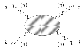
Figure 2: Elastic scattering of longitudinal modes of KK gauge bosons, $n+n\to n+n$, with the gauge index structure $a+b\to c+d$.

Figure 3: The tree-level diagrams contributing to the scattering of massive longitudinal gauge bosons in the SM without a Higgs.

Figure 4: The four diagrams contributing at tree level to the elastic scattering amplitude of the nth KK mode.

Our aim is to build a higgsless model of electroweak symmetry breaking using BC breaking in extra dimensions. However, usually there is a problem in theories with massive gauge bosons without a higgs scalar: the scattering amplitude of longitudinal gauge bosons will grow with the energy and violate unitarity at a low scale. What we would like to first understand is what happens to this unitarity bound in a theory with extra dimensions. For simplicity we will be focusing on the elastic scattering of the longitudinal modes of the n^th KK mode (see fig. 2). The kinematics of this process are determined by the longitudinal polarization vectors and the incoming and outgoing momenta:

$$\epsilon_{\mu}=(\frac{|\vec{p}|}{M},\frac{E}{M}\frac{\vec{p}}{|\vec{p}|})$$

$$p^{in}_{\mu}=(E,0,0,\pm\sqrt{E^{2}-M_{n}^{2}})$$

$$p_{\mu}^{out}=(E,\pm\sqrt{E^{2}-M_{n}^{2}}\sin\theta,0,\pm\sqrt{E^{2}-M_{n}^{2}}\cos\theta).$$ (3.1)

The diagrams that can contribute to this scattering amplitude in a theory with massive gauge bosons (but no scalar Higgs) are given in Fig. 3 (where the $E$-dependence can be estimated from $\epsilon\sim E,p_{\mu}\sim E$ and a propagator $\sim E^{-2}$). This way we find that the amplitude could grow as quickly as $E^{4}$, and then for $E\gg M_{W}$ can expand the amplitude in decreasing powers of $E$ as

$$\mathcal{A}=A^{(4)}\frac{E^{4}}{M_{n}^{4}}+A^{(2)}\frac{E^{2}}{M_{n}^{2}}+A^{(0)}+{\cal O}\left(\frac{M_{n}^{2}}{E^{2}}\right).$$ (3.2)

In the SM (and any theory where the gauge kinetic terms form the gauge invariant combination $F_{\mu\nu}^{2}$) the $A^{(4)}$ term automatically vanishes, while $A^{(2)}$ is only cancelled after taking the Higgs exchange diagrams into account.

In the case of a theory with an extra dimension with BC breaking of the gauge symmetry there are no Higgs exchange diagrams, however one needs to sum up the exchanges of all KK modes, as in Fig. 4. As a result we will find the following expression for the terms in the amplitudes that grow with energy:

$$A^{(4)}=i\left(g^{2}_{nnnn}-\sum_{k}g_{nnk}^{2}\right)\left(f^{abe}f^{cde}(3+6\cos\theta-\cos^{2}\theta)+2(3-\cos^{2}\theta)f^{ace}f^{bde}\right),$$ (3.3)

In order for the term $A^{(4)}$ to vanish it is enough to ensure that the following sum rule among the coupling of the various KK modes is satisfied:

$$g^{2}_{nnnn}=\sum_{k}g_{nnk}^{2}.$$ (3.4)

Assuming $A^{(4)}=0$ we get

$$A^{(2)}=\frac{i}{M_{n}^{2}}\left(4g_{nnnn}M_{n}^{2}-3\sum_{k}g_{nnk}^{2}M_{k}^{2}\right)\left(f^{ace}f^{bde}-\sin^{2}{\textstyle\frac{\theta}{2}}\ f^{abe}f^{cde}\right).$$ (3.5)

Here $g_{nnnn}^{2}$ is the quartic self-coupling of the n^th massive gauge field, while $g_{nnk}$ is the cubic coupling between the KK modes. In theories with extra dimensions these are of course related to the extra dimensional wave functions $f_{n}(y)$ of the various modes as

$$g_{mnk}=g_{5}\int dyf_{m}(y)f_{n}(y)f_{k}(y),$$

$$g^{2}_{mnkl}=g_{5}^{2}\int dyf_{m}(y)f_{n}(y)f_{k}(y)f_{l}(y).$$ (3.6)

The most important point about the amplitudes in (3.3-3.5) is that they only depend on an overall kinematic factor multiplied by an overall expression of the couplings. Assuming that the relation (3.4) holds we can find a sum rule that ensures the vanishing of the $A^{(2)}$ term:

$$g_{nnnn}M_{n}^{2}=\frac{3}{4}\sum_{k}g_{nnk}^{2}M_{k}^{2}$$ (3.7)

Amazingly, higher dimensional gauge invariance will ensure that both of these sum rules are satisfied as long as the breaking of the gauge symmetry is spontaneous. For example, it is easy to show the first sum rule via the completeness of the wave functions $f_{n}(y)$:

$$\int_{0}^{\pi R}dy\,f_{n}^{4}(y)=\sum_{k}\int_{0}^{\pi R}dy\int_{0}^{\pi R}dz\ f_{n}^{2}(y)f_{n}^{2}(z)f_{k}^{\vphantom{2}}(y)f_{k}^{\vphantom{2}}(z),$$ (3.8)

and using the completeness relation

$$\sum_{k}f_{k}(y)f_{k}(z)=\delta(y-z),$$ (3.9)

we can see that the two sides will indeed agree. One can similarly show that the second sum rule will also be satisfied if the boundary conditions are natural ones (as defined in Section 2) and all terms in the Lagrangian (including boundary terms) are gauge invariant.

What we see from the above analysis is that in any gauge invariant extra dimensional theory the terms in the amplitude that grow with the energy will cancel. However, this will not automatically mean that the theory itself is unitary. The reason is that there are two additional worries: even if $A^{(4)}$ and $A^{(2)}$ vanish $A^{(0)}$ could be too large and spoil unitarity. This is what happens in the SM if the Higgs mass is too large. In the extra dimensional case what this would mean is that the extra KK modes would make the scattering amplitude flatten out to a constant value. However if the KK modes themselves are too heavy then this flattening out will happen too late when the amplitude already violates unitarity. The other issue is that in a theory with extra dimensions there are infinitely many KK modes and thus as the scattering energy grows one should not only worry about the elastic channel, but the ever growing number of possible inelastic final states. The full analysis taking into account both effects has been performed in [34], where it was shown that after taking into account the opening up of the inelastic channels the scattering amplitude will grow linearly with energy, and will always violate unitarity at some energy scale. This is a consequence of the intrinsic non-renormalizability of the higher dimensional gauge theory. It was found in [34] that the unitarity violation scale due to the linear growth of the scattering amplitude is equal (up to a small numerical factor of order $2-4$) to the cutoff scale of the 5D theory obtained from naive dimensional analysis (NDA). This cutoff scale can be estimated in the following way. The one-loop amplitude in 5D is proportional to the 5D loop factor

$$\frac{g_{5}^{2}}{24\pi^{3}}.$$ (3.10)

The dimensionless quantity obtained from this loop factor is

$$\frac{g_{5}^{2}E}{24\pi^{3}},$$ (3.11)

where $E$ is the scattering energy. The cutoff scale can be obtained by calculating the energy scale at which this loop factor will become order one (that is the scale at which the loop and tree-level contributions become comparable). From this we get

$$\Lambda_{NDA}=\frac{24\pi^{3}}{g_{5}^{2}}.$$ (3.12)

We can express this scale using the matching of the higher dimensional and the lower dimensional gauge couplings. In the simplest theories this is usually given by

$$g_{5}^{2}=\pi Rg_{4}^{2},$$ (3.13)

where $\pi R$ is the length of the interval, and $g_{4}$ is the effective 4D gauge coupling. So the final expression of the cutoff scale can be given as

$$\Lambda_{NDA}=\frac{24\pi^{2}}{g_{4}^{2}R}.$$ (3.14)

We will see that in the Higgsless models $1/R$ will be replaced by $M_{W}^{2}/M_{KK}$, where $M_{W}$ is the physical W mass, and $M_{KK}$ is the mass of the first KK mode beyond the W. Thus the cutoff scale will indeed be lower if the mass of the KK mode used for unitarization is higher. However, this $\Lambda_{NDA}$ could be significantly higher than the cutoff scale in the SM without a Higgs, which is around 1.8 TeV. We will come back to a more detailed discussion of $\Lambda_{NDA}$ in higgsless models at the end of this section.

3.2 Naive Higgsless toy model

Now that we have convinced ourselves that one can use KK gauge bosons to delay the unitarity violation scale basically up to the cutoff scale of the higher dimensional gauge theory, we should start looking for a model that actually has these properties and resembles the SM. It should have a massless photon, a massive charged gauge boson to be identified with the $W$ and a somewhat heavier neutral gauge boson to be identified with the $Z$. Most importantly, we need to have the correct SM mass ratio (at tree-level)

$$\frac{M_{W}^{2}}{M_{Z}^{2}}=\cos^{2}\theta_{W}=\frac{g^{2}}{g^{2}+g^{\prime 2}},$$ (3.15)

where $g$ is the SU(2)_L gauge coupling and $g^{\prime}$ the U(1)_Y gauge coupling of the SM. We would like to use BC’s to achieve this. This seems to be very hard at first sight, since we need to somehow get a theory where the masses of the KK modes are related to the gauge couplings. Usually the KK masses are simply integer or half-integer multiples of $1/R$. For example, if we look at a very naive toy model with an SU(2) gauge group in the bulk, we could consider the following BC’s for the various gauge directions:

$$\partial_{y}A^{3}_{\mu}=0\ {\rm at}\ y=0,\pi R,$$

$$\partial_{y}A^{1,2}_{\mu}=0\ {\rm at}\ y=0$$

$$A^{1,2}_{\mu}=0\ {\rm at}\ y=\pi R.$$ (3.16)

With these BC’s the wave functions for the various gauge fields will be for $A^{3}$

$$f^{(n)}_{3}(y)=\cos\frac{ny}{R}$$ (3.17)

while for the $1,2$ directions

$$f^{(m)}_{1,2}(y)=\cos\frac{(2m+1)y}{2R}$$ (3.18)

The mass spectrum then is

$$A^{3}\to m_{n}=\frac{n}{R},\ \ 0,\frac{1}{R},\frac{2}{R},\ldots$$

$$A^{1,2}\to m_{m}=\frac{m+\frac{1}{2}}{R},\ \ \frac{1}{2R},\frac{3}{2R},\ldots$$ (3.19)

This spectrum somewhat resembles that of the SM in the sense that there is a massless gauge boson that can be identified with the $\gamma$, a pair of charged massive gauge bosons that can be identified with the $W^{\pm}$, and a massive neutral gauge boson that can be identified with the $Z$. However, we can see that the mass ratio of the W and Z is given by

$$\frac{M_{Z}}{M_{W}}=2,$$ (3.20)

and another problem is that the first KK mode of the W,Z is given by

$$\frac{M_{Z^{\prime}}}{M_{Z}}=2,\ \ \frac{M_{W^{\prime}}}{M_{W}}=3.$$ (3.21)

Thus, besides getting the totally wrong W/Z mass ratio there would also be additional KK states at masses of order 250 GeV, which is phenomenologically unacceptable. We will see that both of these problems can be resolved by going to a warped higgsless model with custodial SU(2).

3.3 Custodial SU(2) and flat space higgsless model

We have seen above that a major question in building a realistic higgsless model is how to ensure that the W/Z mass ratio agrees with the tree-level result. Let us first understand why the tree result in the SM is given by

$$\rho\equiv\frac{M_{W}^{2}}{\cos^{2}\theta_{W}M_{Z}^{2}}=1.$$ (3.22)

The electroweak symmetry in the SM is broken by the Higgs scalar $H$, which transforms as a ${\bf 2}_{\frac{1}{2}}$ under SU(2)${}_{L}\times$ U(1)_Y. The Higgs potential is given by

$$V(H)=-\mu^{2}H^{\dagger}H+\lambda(H^{\dagger}H)^{2}.$$ (3.23)

This potential is only a function of $H^{\dagger}H$, which can also be written as

$$H^{\dagger}H=h_{1}^{2}+h_{2}^{2}+h_{3}^{2}+h_{4}^{2},$$ (3.24)

where the Higgs doublet has been written in terms of its real and imaginary components as

$$H=\left(\begin{array}[]{c}h_{1}+ih_{2}\\ h_{3}+ih_{4}\end{array}\right).$$ (3.25)

We can see from (3.24) that the Higgs potential actually has a bigger global symmetry than SU(2)${}_{L}\times$ U(1)_Y: it is invariant under the full SO(4) rotation of the four independent real fields in the Higgs doublet. The SO(4) group is actually not a simple group, but rather equivalent to SU(2)${}_{L}\times$SU(2)_R. The origin of the SU(2)_R symmetry can also be understood as follows. A doublet of SU(2) is a pseudo-real representation, which means that the complex conjugate of the doublet is equivalent to the doublet itself. The way this manifests itself is if we consider the doublet to be a field with a lower SU(2) index $H_{i}$, then the complex conjugate would automatically have an upper index. However, using the SU(2) epsilon $\epsilon_{ij}$ this can be lowered again, and so $H_{i}$ and $i\epsilon_{ij}(H^{*})^{j}$ transform in the same way. This means that in addition to an SU(2)_L acting on the usual SU(2) index, there is another SU(2) symmetry that mixes $H$ with $\epsilon H^{*}$. To make this more intuitive, we could write a 2 by 2 matrix as

$$\left(\begin{array}[]{cc}H&\epsilon H^{*}\end{array}\right),$$ (3.26)

and then the ordinary SU(2)_L would act from the left, and the additional SU(2)_R would be a global symmetry acting on this matrix from the right.

Once the Higgs scalar gets a VEV, it will break the SO(4) global symmetry to an SO(3) subgroup. In the SU(2) language this means that SU(2)${}_{L}\times$SU(2)_R is broken to the diagonal subgroup $SU(2)_{D}$. This is most easily seen from the representation in (3.26) since then we have a matrix whose VEV is given by ${\rm diag}(v,v)$, and obviously leaves the diagonal subgroup unbroken.

The claim is that once such an SU(2)_D subgroup (which is usually referred to as the custodial SU(2) symmetry of the Higgs potential) is left unbroken during electroweak symmetry breaking, it is guaranteed that the $\rho$-parameter will come out to be one at tree level. Let us quickly prove that this is indeed the case. The generic description of the global symmetry breaking pattern SU(2)${}_{L}\times$ SU(2)${}_{R}\to$ SU(2)_D can be achieved via the non-linear $\sigma$-model which will describe the physics of the 3 Goldstone-modes appearing in this symmetry breaking. In this description the possible massive Higgs modes are integrated out. This model will give all the consequences of the global symmetries. In this model the Goldstone fields are represented by a 2 by 2 unitary matrix $\Sigma$, which is given in terms of the Goldstone modes $\pi^{a}$ as

$$\Sigma=e^{i\frac{\pi^{a}\tau^{a}}{f}},$$ (3.27)

and transforms under SU(2)${}_{L}\times$SU(2)_R as $\Sigma\to U_{L}\Sigma U_{R}^{\dagger}$. One can think of the SU(2)${}_{L}\times$ U(1)_Y electroweak symmetries as a subgroup of SU(2)${}_{L}\times$ SU(2)_R, with U(1)${}_{Y}\subset$ SU(2)_R. This gauging of a subgroup of the global symmetries will explicitly break some of the global symmetries, but this is easily incorporated into the non-linear $\sigma$-model description. (Note, that in the presence of fermions the global symmetry needs to be enlarged to SU(2)${}_{L}\times$ SU(2)${}_{R}\times$ U(1)_B-L, and then U(1)${}_{Y}\subset$ SU(2)${}_{R}\times$U(1)_B-L, where U(1)_B-L is the baryon number minus lepton number symmetry.) The covariant derivative is then given by

$$D_{\mu}=\partial_{\mu}-ig\frac{\tau^{a}}{2}A_{\mu}^{a}-i\frac{g^{\prime}}{2}B_{\mu}.$$ (3.28)

The leading kinetic term for the pions is given by

$$f^{2}{\rm Tr}(D_{\mu}\Sigma^{\dagger})(D^{\mu}\Sigma).$$ (3.29)

Expanding this expression in the pion fluctuations will result in mass terms for the gauge fields

$$M_{W}^{2}=\frac{g^{2}f^{2}}{4},\ \ M_{Z}^{2}=\frac{(g^{2}+g^{\prime 2})f^{2}}{4},$$ (3.30)

and thus

$$\frac{M_{W}^{2}}{M_{Z}^{2}}=\frac{g^{2}}{g^{2}+g^{\prime 2}}.$$ (3.31)

Note, that in the above derivation the only information that has been used was the global symmetry breaking pattern SU(2)${}_{L}\times$SU(2)${}_{R}\to$ SU(2)_D, with the appropriate subgroup being gauged. Once this symmetry breaking pattern is established, it is guaranteed that the tree-level prediction for the $\rho$-parameter will be 1.

From the above discussion it is clear that in order to find a higgsless model with the correct W/Z mass ratio one needs to find an extra dimensional model that has the custodial SU(2) symmetry incorporated [17]. Once such a construction is found, the gauge boson mass ratio will automatically be the right one. Therefore we need to somehow involve SU(2)_R in the construction. The simplest possibility is to put an entire SU(2)${}_{L}\times$SU(2)${}_{R}\times$U(1)_B-L gauge group in the bulk of an extra dimension [9]. In order to mimic the symmetry breaking pattern in the SM most closely, we assume that on one of the branes the symmetry breaking is SU(2)${}_{L}\times$SU(2)${}_{R}\to$ SU(2)_D, with $U(1)_{B-L}$ unbroken. On the other boundary one needs to reduce the bulk gauge symmetry to that of the SM, and thus have a symmetry breaking pattern SU(2)${}_{R}\times$U(1)${}_{B-L}\to$ U(1)_Y, which is illustrated in Fig. 5.

Figure 5: The symmetry breaking structure of the flat space higgsless toy model.

We denote by $A^{R\,a}_{M}$, $A^{L\,a}_{M}$ and $B_{M}$ the gauge bosons of $SU(2)_{R}$, $SU(2)_{L}$ and $U(1)_{B-L}$ respectively; $g_{5L}$ and $g_{5R}$ are the the gauge couplings of the two $SU(2)$’s and $\tilde{g}_{5}$, the gauge coupling of the $U(1)_{B-L}$. In order to obtain the desired BC’s as discussed above we need to follow the procedure laid out in the first lecture. We assume that there is a boundary Higgs on the left brane in the representation $(1,2)_{\frac{1}{2}}$ under SU(2)${}_{L}\times$SU(2)${}_{R}\times$U(1)_B-L, which will break SU(2)${}_{R}\times$U(1)_B-L to U(1)_Y. We could also use the more conventional triplet representation under SU(2)_R which will allow us to get neutrino masses later on. On the right brane we assume that there is a bi-doublet higgs in the representation $(2,2)_{0}$ which breaks the electroweak symmetry as in the SM: SU(2)${}_{L}\times$SU(2)${}_{R}\to$SU(2)_D. We will then take all the Higgs VEV’s to infinity in order to decouple the boundary scalars from the theory, and impose the natural boundary conditions as described in the first lecture. The BC’s we will arrive at then are:

$${\rm at}\ y=0: \left\{\begin{array}[]{l}\partial_{z}(g_{5R}B_{\mu}+\tilde{g}_{5}A_{\mu}^{R3})=0\ ,\partial_{z}A^{La}_{\mu}=0,\ A_{\mu}^{R1,2}=0,\\ \vrule height=15.0pt,depth=5.0pt,width=0.0pt\tilde{g}_{5}B_{\mu}-g_{5R}A_{\mu}^{R3}=0,\end{array}\right.$$ (3.34)

$${\rm at}\ y=\pi R: \left\{\begin{array}[]{l}\partial_{z}(g_{5R}A^{L\,a}_{\mu}+g_{5L}A^{R\,a}_{\mu})=0,\ \partial_{z}B_{\mu}=0,\ g_{5L}A^{L\,a}_{\mu}-g_{5R}A^{R\,a}_{\mu}=0.\end{array}\right.$$ (3.36)

The BC’s for the $A_{5}$ and $B_{5}$ components will be the opposite of the 4D gauge fields as usual, i.e. all Dirichlet conditions should be replaced by Neumann and vice versa. The next step to determine the mass spectrum is to find the right KK decomposition of this model. First of all, none of the $A_{5}$ and $B_{5}$ components have a flat BC on both ends. This means that there will be no zero mode in these fields, and as we have seen all the massive scalars are unphysical, since they are just gauge artifacts (supplying the longitudinal components of the massive KK towers). So we will not need to discuss the modes in these fields. The main point to observe about the KK decomposition of the gauge fields is that the BC’s will mix up the states in the various components. This will imply that a single 4D mode will live in several different 5D fields. Since in the bulk there is no mixing, and we are discussing at the moment a flat 5D background, the wave functions will be of the form $f_{k}(z)\propto a\cos M_{k}z+b\sin M_{k}z$. If we make the simplifying assumption that $g_{5L}=g_{5R}$, then the KK decomposition will be somewhat simpler than the most generic one, and given by (we denote by $A^{L,R\,\pm}_{\mu}$ the linear combinations ${\textstyle\frac{1}{\sqrt{2}}}(A^{L,R\,1}\mp iA^{L,R\,2})$):

$$B_{\mu}(x,y) = g\,a_{0}\gamma_{\mu}(x)+{g^{\prime}}\sum_{k=1}^{\infty}b_{k}\cos(M^{Z}_{k}y)\,Z^{(k)}_{\mu}(x)\,,$$ (3.37)

$$A^{L\,3}_{\mu}(x,y) = {g^{\prime}}\,a_{0}\gamma_{\mu}(x)-g\sum_{k=1}^{\infty}b_{k}\frac{\cos(M^{Z}_{k}(y-\pi R))}{2\cos(M^{Z}_{k}\pi R)}\,Z^{(k)}_{\mu}(x)\,,$$ (3.38)

$$A^{R\,3}_{\mu}(x,y) = {g^{\prime}}a_{0}\gamma_{\mu}(x)-g\sum_{k=1}^{\infty}b_{k}\frac{\cos(M^{Z}_{k}(y+\pi R))}{2\cos(M^{Z}_{k}\pi R)}\,Z^{(k)}_{\mu}(x)\,,$$ (3.39)

$$A^{L\,\pm}_{\mu}(x,y) = \sum_{k=1}^{\infty}c_{k}\cos(M^{W}_{k}(y-\pi R))\,W^{(k)\,\pm}_{\mu}(x)\,,$$ (3.40)

$$A^{R\,\pm}_{\mu}(x,y) = \sum_{k=1}^{\infty}c_{k}\cos(M^{W}_{k}(y+\pi R))\,W^{(k)\,\pm}_{\mu}(x)\,.$$ (3.41)

The coefficients and the masses are then determined by imposing the BC’s on this KK decomposition. The resulting mass spectrum that we find is the following. The spectrum is made up of a massless photon, the gauge boson associated with the unbroken $U(1)_{Q}$ symmetry, and some towers of massive charged and neutral gauge bosons, $W^{(k)}$ and $Z^{(k)}$ respectively. The masses of the $W^{\pm}$’s are given by

$$M^{W}_{k}=\frac{2k-1}{4R},\ \ k=1,2\ldots$$ (3.42)

while for $Z$’s there are two towers of neutral gauge bosons with masses

$$M^{Z}_{k}=\left(M_{0}+\frac{k-1}{R}\right),\ \ k=1,2\ldots$$ (3.43)

$$M^{Z^{\prime}}_{k}=\left(-M_{0}+\frac{k}{R}\right),\ \ k=1,2\ldots$$ (3.44)

where $M_{0}={\textstyle\frac{1}{\pi R}}\arctan\sqrt{1+2{{g^{\prime}}}^{2}/g^{2}}$. Note that $1/(4R)<M_{0}<1/(2R)$ and thus the $Z^{\prime}$’s are heavier than the $Z$’s ($M^{Z^{\prime}}_{k}>M^{Z}_{k}$). We also get that the lightest $Z$ is heavier than the lightest $W$ ($M^{Z}_{1}>M^{W}_{1}$), in agreement with the SM spectrum. However, the mass ratio of W/Z is given by

$$\frac{M_{W}^{2}}{M_{Z}^{2}}=\frac{\pi^{2}}{16}\arctan^{-2}\sqrt{1+\frac{g_{4D}^{{}^{\prime}2}}{g_{4D}^{2}}}\sim 0.85,$$ (3.45)

and hence the $\rho$ parameter is

$$\rho=\frac{M_{W}^{2}}{M_{Z}^{2}\cos^{2}\theta_{W}}\sim 1.10\ .$$ (3.46)

Thus the mass ratio is close to the SM value, however the ten percent deviation is still huge compared to the experimental precision. The reason for this deviation is that while the bulk and the right brane are symmetric under custodial SU(2), the left brane is not, and the KK wave functions do have a significant component around the left brane, which will give rise to the large deviation from $\rho=1$. Thus one needs to find a way of making sure that the KK modes of the gauge fields do not very much feel that left brane, but are repelled from there, and only the lightest (almost zero modes) $\gamma,Z,W^{\pm}$ will have a large overlap with the left brane.

3.4 The AdS/CFT correspondence

We have seen above that one would need to modify the flat space setup such that the KK modes get pushed away from the left brane without breaking any new symmetries. There are two possible ways that this can be done (and in fact we will see that these two are basically equivalent to each other). One possibility is to simply add a large brane kinetic term for the gauge fields on the left brane where custodial SU(2) is violated [20]. The effect of this will be exactly to push away the heavy KK modes (since as we have seen in the first lecture the BC does depend on the eigenvalue). This way the custodial SU(2) can be approximately restored in the KK sector of the theory. The second possibility which we will be pursuing here is to use the AdS/CFT correspondence. This has been first pointed out in [17].

It has been realized by Maldacena [43] in 1997 that certain string theories on an anti-de Sitter (AdS) background are actually equivalent to some 4D conformal field theories. The crucial ingredient was that the conformal group SO(2,4) is equivalent to the isometries of 5D AdS space, whose metric is given by

$$ds^{2}=\left(\frac{R}{z}\right)^{2}\Big{(}\eta_{\mu\nu}dx^{\mu}dx^{\nu}-dz^{2}\Big{)}$$ (3.47)

where $0<z<\infty$ is the radial AdS coordinate. Basically the point is that besides the usual 5D Poincare transformations this metric has an additional rescaling invariance $z\to\alpha z,x_{\mu}\to\alpha x_{\mu}$. Using several checks Maldacena was able to gather convincing evidence that ${\cal N}=4$ supersymmetric Yang Mills theory in a certain limit is equivalent to type IIB string theory on AdS${}_{5}\times S^{5}$. This field theory is automatically conformal due to the number of supercharges. One crucial observation is that the coordinate along the AdS direction actually corresponds to an energy scale in the CFT. This is quite clear from the above mentioned rescaling invariance. Rescaling $z$ implies rescaling $x$. But rescaling $x$ means changing the energy scale in the CFT. So this will imply that the $z\to 0$ region corresponds to the most energetic sector of the CFT $E\to\infty$, while the $z\to\infty$ corresponds to low energies $E\to 0$. The other important observation of this equivalence is that the field theory has a large global symmetry SU(4)_R. The way this is realized in the string theory side is that SO(6)$=$SU(4) is the isometry of the 5D sphere $S^{5}$. Thus there will be massless gauge boson corresponding to this SU(4) global symmetry in the AdS₅ theory. What this seems to suggest is that the AdS₅ bulk is really supplying the modes of the CFT itself, while the global symmetries of the CFT will manifest themselves in gauge fields appearing in the 5D theory. One final crucial ingredient needed for us is how this correspondence will be modified if the AdS space is not infinite, but we are considering only a finite interval (slice) of 5D AdS space. In this case we clearly do not have the full conformal invariance, since the appearance of the boundaries of the slice of AdS will explicitly break it. One way of interpreting the appearance of a boundary close to $z=0$ (usually called the UV brane or Planck brane since it corresponds to high energies) is that the field theory has an explicit cutoff corresponding to this energy scale. If the cutoff is at $z=R$, the field theory will have a UV cutoff $\Lambda=\frac{1}{R}$. The interpretation of the other boundary (usually referred to as IR brane or TeV brane) is trickier. It has been argued in [44, 45] that the proper interpretation of such an IR brane is that the CFT spontaneously breaks the conformal invariance at low energies. The location of the IR brane will supply an IR cutoff. For those familiar with the phenomenology of the Randall-Sundrum models, this can be explained by realizing that the KK spectrum of the fields will be localized on this IR brane. In the presence of the IR brane there will also be a discrete spectrum for these KK modes. These discrete KK modes can be thought of as the composites (bound states) formed by the CFT after it breaks conformality and becomes strongly interacting (confining). The analogy could be a theory that is very slowly running (its $\beta$-function is very close to zero), then after a long period of slow running (“walking”) the theory will become strongly interacting, and the theory will confine (if it is QCD-like) and form bound states. What happens then to the gauge fields if they are in the bulk of a finite slice of the AdS space? It depends on their BC’s. The main difference between the full AdS and the case of a slice is that while a gauge field zero mode is not normalizable in an infinite AdS space, it will become normalizable in the case of a slice. So this means that if there is a zero mode present, then one would need to identify this as a weakly gauged global symmetry of the CFT. Whether the gauge field in the finite slice actually has a zero mode or not, depends on its BC’s. If it has Dirichlet BC on the UV brane, then the zero mode will pick up a mass of the order of the scale at the UV brane (that is proportional to the UV cutoff), so it will be totally eliminated from the theory. Thus in this case even in a finite slice the symmetry should be thought of as a global symmetry only. However, if the BC on the UV brane is Neumann, while on the IR brane is Dirichlet, then the zero mode picks up a mass of the order of the IR cutoff (the confinement scale, the KK scale of the other resonances), so the way this should be interpreted is that the CFT became strongly interacting, and that breaking of conformality also resulted in breaking the weakly gauged global symmetry spontaneously. Later on it was also realized that perhaps supersymmetry may not be necessary for such a correspondence to exist. So let us summarize the rules laid out above for the AdS/CFT correspondence (at least the ones relevant for model building) in Table 1.

Bulk of AdS	$\leftrightarrow$	CFT
Coordinate ($z$) along AdS	$\leftrightarrow$	Energy scale in CFT
Appearance of UV brane	$\leftrightarrow$	CFT has a cutoff
Appearance of IR brane	$\leftrightarrow$	conformal symmetry broken spontaneously by CFT
KK modes localized on IR brane	$\leftrightarrow$	composites of CFT
Modes on the UV brane	$\leftrightarrow$	Elementary fields coupled to CFT
Gauge fields in bulk	$\leftrightarrow$	CFT has a global symmetry
Bulk gauge symmetry broken on UV brane	$\leftrightarrow$	Global symmetry not gauged
Bulk gauge symmetry unbroken on UV brane	$\leftrightarrow$	Global symmetry weakly gauged
Higgs on IR brane	$\leftrightarrow$	CFT becoming strong produces composite Higgs
Bulk gauge symmetry broken on IR brane by BC’s	$\leftrightarrow$	Strong dynamics that breaks CFT also breaks gauge symmetry

Table 1: Relevant rules for model building using the AdS/CFT correspondence

Using the rules of the correspondence found in Table 1 we can now relatively easily find the theory that we are after. We want a theory that has an $SU(2)_{L}\times SU(2)_{R}\times U(1)_{B-L}$ global symmetry, with the $SU(2)_{L}\times U(1)_{Y}$ subgroup weakly gauged, and broken by BC’s on the IR brane. To have the full global symmetry, we need to take $SU(2)_{L}\times SU(2)_{R}\times U(1)_{B-L}$ in the bulk of AdS₅. To make sure that we do not get unwanted gauge fields at low energies, we need to break $SU(2)_{R}\times U(1)_{B-L}$ to $U(1)_{Y}$ on the UV brane, which we will do by BC’s as in the flat case. Finally, the boundary conditions on the TeV brane break $SU(2)_{L}\times SU(2)_{R}$ to $SU(2)_{D}$, thus providing for electroweak symmetry breaking. This setup is illustrated in Fig. 6. Note, that it is practically identical to the flat space toy model considered before, except that the theory is in AdS space.

Figure 6: The symmetry breaking structure of the warped higgsless model.

3.5 The warped space higgsless model

Before coming to the detailed prediction of the mass spectrum of the warped space higgsless model outlined above, let us first briefly discuss how to deal with a gauge theory in an AdS background [46, 47]. We will be considering a 5D gauge theory in the fixed gravitational background

$$ds^{2}=\left(\frac{R}{z}\right)^{2}\Big{(}\eta_{\mu\nu}dx^{\mu}dx^{\nu}-dz^{2}\Big{)}$$ (3.48)

where $z$ is on the interval $[R,R^{\prime}]$. We will not be considering gravitational fluctuations, that is we are assuming that the Planck scale is sent to infinity, while the background is frozen to be the one given above. In RS-type models $R$ is typically $\sim 1/M_{Pl}$ and $R^{\prime}\sim{\rm TeV}^{-1}$. For higgsless models we will see later on what the optimal choice for these scales are. The action for a gauge theory on a fixed background will be given by

$$S=\int d^{5}x\sqrt{g}\left[-\frac{1}{4}F_{MN}^{a}F_{PQ}^{a}g^{MP}g^{NQ}\right]$$ (3.49)

Putting in the metric (3.48) we find

$$S=\int d^{4}x\int_{R}^{R^{\prime}}\frac{R}{z}\left[-\frac{1}{4}{F_{\mu\nu}^{a}}^{2}-\frac{1}{2}{F_{\mu 5}^{a}}^{2}\right].$$ (3.50)

To get the right gauge fixing term, we have to repeat the procedure from the first section. The mixing term between $A_{\mu}$ and $A_{5}$ is given by

$$\int d^{4}x\int_{R}^{R^{\prime}}dz\frac{R}{z}\partial_{\mu}\partial^{5}A^{\mu}=-\int d^{4}x\int_{R}^{R^{\prime}}dz\partial_{\mu}A^{\mu}\partial_{5}\left(\frac{R}{z}A_{5}\right).$$ (3.51)

In the second equality we have integrated by parts and neglected a boundary term (which is necessary for determining the BC’s, however these will not change due to the presence of the warping so the BC’s derived for the flat space model will be applicable here as well). This implies that the gauge fixing term necessary in the warped case is given by

$$S_{gf}=-\int d^{4}x\int_{R}^{R^{\prime}}dz\frac{1}{2\xi}\frac{R}{z}\left[\partial_{\mu}A^{\mu}-\xi\frac{z}{R}\partial_{5}\left(\frac{R}{z}A_{5}\right)\right]^{2}.$$ (3.52)

Due to the chosen BC’s the $A_{5}$ fields will have no zero modes they will all again become massive gauge artifacts and can be eliminated in the unitary gauge. The quadratic piece of the action for the gauge fields will be then given by

$$\int d^{4}x\int_{R}^{R^{\prime}}dz\frac{R}{z}\frac{1}{2}A_{\mu}\left[\left(\partial^{2}-\frac{z}{R}\partial_{z}\left(\frac{R}{z}\partial_{z}\right)\right)\eta^{\mu\nu}-\left(1-\frac{1}{\xi}\right)\partial^{\mu}\partial^{\nu}\right]A_{\nu}.$$ (3.53)

As before, we go to $4D$ momentum space by writing $A_{\mu}(x,z)=\epsilon_{\mu}(p)f(z)e^{ip\cdot x}$. The equation of motion for the wave function $f(z)$ will then become ($p^{2}=M^{2}$):

$$\left[-M^{2}-z\partial_{5}\left(\frac{1}{z}\partial_{5}\right)\right]f(z)=0.$$ (3.54)

Equivalently it can be written as

$$f^{\prime\prime}-\frac{1}{z}f^{\prime}+M^{2}f=0.$$ (3.55)

This will lead to a Bessel equation for $g(z)$ after the substitution $f(z)=zg(z)$:

$$g^{\prime\prime}+\frac{1}{z}g^{\prime}+(M^{2}-\frac{1}{z^{2}})g=0,$$ (3.56)

which is a Bessel equation of order 1. The solution is of the form

$$f(z)=z\left(AJ_{1}(q_{k}z)+BY_{1}(q_{k}z)\right).$$ (3.57)

The BC’s corresponding to the symmetry breaking pattern discussed above for the warped higgsless model are identical to the ones for the flat space case [18]:

$${\rm at}\ y=0: \left\{\begin{array}[]{l}\partial_{z}(g_{5R}B_{\mu}+\tilde{g}_{5}A_{\mu}^{R3})=0\ \partial_{z}A^{La}_{\mu}=0,\ A_{\mu}^{R1,2}=0,\\ \vrule height=15.0pt,depth=5.0pt,width=0.0pt\tilde{g}_{5}B_{\mu}-g_{5R}A_{\mu}^{R3}=0,\end{array}\right.$$ (3.60)

$${\rm at}\ y=\pi R: \left\{\begin{array}[]{l}\partial_{z}(g_{5R}A^{L\,a}_{\mu}+g_{5L}A^{R\,a}_{\mu})=0,\ \partial_{z}B_{\mu}=0,\ g_{5L}A^{L\,a}_{\mu}-g_{5R}A^{R\,a}_{\mu}=0.\end{array}\right.$$ (3.62)

Again the BC’s for the $A_{5}$’s are the opposite to that of the corresponding combination of the $4D$ gauge fields, and these BC’s can be thought of as arising from Higgses on each brane in the large VEV limit. Using the above Bessel functions the KK mode expansion is given by the solutions to this equation which are of the form

$$\psi^{(A)}_{k}(z)=z\left(a^{(A)}_{k}J_{1}(q_{k}z)+b^{(A)}_{k}Y_{1}(q_{k}z)\right)~{},$$ (3.63)

where $A$ labels the corresponding gauge boson. Due to the mixing of the various gauge groups, the KK decomposition is slightly complicated but it is obtained by simply enforcing the BC’s:

$$B_{\mu}(x,z) = g_{5}\,a_{0}\gamma_{\mu}(x)+\sum_{k=1}^{\infty}\psi^{(B)}_{k}(z)\,Z^{(k)}_{\mu}(x)\,,$$ (3.64)

$$A^{L\,3}_{\mu}(x,z) = {\tilde{g}_{5}}\,a_{0}\gamma_{\mu}(x)+\sum_{k=1}^{\infty}\psi^{(L3)}_{k}(z)\,Z^{(k)}_{\mu}(x)\,,$$ (3.65)

$$A^{R\,3}_{\mu}(x,z) = {\tilde{g}_{5}}\,a_{0}\gamma_{\mu}(x)+\sum_{k=1}^{\infty}\psi^{(R3)}_{k}(z)\,Z^{(k)}_{\mu}(x)\,,$$ (3.66)

$$A^{L\,\pm}_{\mu}(x,z) = \sum_{k=1}^{\infty}\psi^{(L\pm)}_{k}(z)\,W^{(k)\,\pm}_{\mu}(x)\,,$$ (3.67)

$$A^{R\,\pm}_{\mu}(x,z) = \sum_{k=1}^{\infty}\psi^{(R\pm)}_{k}(z)\,W^{(k)\,\pm}_{\mu}(x)\,.$$ (3.68)

Here $\gamma(x)$ is the 4D photon, which has a flat wavefunction due to the unbroken $U(1)_{Q}$ symmetry, and $W^{(k)\,\pm}_{\mu}(x)$ and $Z^{(k)}_{\mu}(x)$ are the KK towers of the massive $W$ and $Z$ gauge bosons, the lowest of which are supposed to correspond to the observed $W$ and $Z$.

To leading order in $1/R$ and for $\log\left(R^{\prime}/R\right)\gg 1$, the lightest solution for this equation for the mass of the $W^{\pm}$’s is

$$M_{W}^{2}\approx\frac{1}{R^{\prime 2}\log\left(\frac{R^{\prime}}{R}\right)}\,.$$ (3.69)

Note, that this result does not depend on the 5D gauge coupling, but only on the scales $R,R^{\prime}$. Taking $R=10^{-19}$ GeV^-1 will fix $R^{\prime}=2\cdot 10^{-3}$ GeV^-1. The lowest mass of the $Z$ tower is approximately given by

$$M_{Z}^{2}=\frac{g_{5}^{2}+2\tilde{g}_{5}^{2}}{g_{5}^{2}+\tilde{g}_{5}^{2}}\frac{1}{R^{\prime 2}\log\left(\frac{R^{\prime}}{R}\right)}\,.$$ (3.70)

If the SM fermions are localized on the Planck brane then the leading order expression for the effective 4D couplings will be given by (see Section 5 for more details)

$$\frac{1}{g^{2}}=\frac{R\log\left(\frac{R^{\prime}}{R}\right)}{g_{5}^{2}}$$

$$\frac{1}{g^{\prime 2}}=R\log\left(\frac{R^{\prime}}{R}\right)\left(\frac{1}{g_{5}^{2}}+\frac{1}{\tilde{g}_{5}^{2}}\right),$$ (3.71)

thus the 4D Weinberg angle will be given by

$$\sin\theta_{W}=\frac{\tilde{g}_{5}}{\sqrt{g_{5}^{2}+2\tilde{g}_{5}^{2}}}=\frac{g^{\prime}}{\sqrt{g^{2}+g^{\prime 2}}}.$$ (3.72)

We can see that to leading order the SM expression for the W/Z mass ratio is reproduced in this theory as expected. In fact the full structure of the SM coupling is reproduced at leading order in $1/\log(R^{\prime}/R)$, which implies that at the leading log level there is no $S$-parameter either. An $S$-parameter in this language would have manifested itself in an overall shift of the coupling of the Z compared to its SM value evaluated from the $W$ and $\gamma$ couplings, which are absent at this order of approximation. The corrections to the SM relations will appear in the next order of the log expansion. Since $\log\left(\frac{R^{\prime}}{R}\right)\sim{\cal O}(10)$, this correction could still be too large to match the precision electroweak data. We will be discussing the issue of electroweak precision observables in the last lecture.

The KK masses of the W (and the Z bosons as well due to custodial SU(2) symmetry) will be given approximately by

$$m_{W_{n}}=\frac{\pi}{2}(n+\frac{1}{2})\frac{1}{R^{\prime}},\ \ n=1,2,\ldots.$$ (3.73)

We can see that the ratio between the physical W mass and the first KK mode is given by

$$\frac{m_{W}}{m_{W}^{\prime}}=\frac{4}{3\pi}\frac{1}{\sqrt{\log\left(\frac{R^{\prime}}{R}\right)}}.$$ (3.74)

We can see that warping will achieve two desirable properties: it will enforce custodial SU(2) and thus automatically generate the correct W/Z mass ratio, but it will also push up the masses of the KK resonances of the W and Z. This will imply that we can get a theory where the W’, Z’ bosons are not so light that they would already be excluded by the LEP or the Tevatron experiments. Finally, we can return to the issue of perturbative unitarity in these models. In the flat space case we have seen that the scale of unitarity violation is basically given by the NDA cutoff scale (3.12). However, in a warped extra dimension all scales will be dependent on the location along the extra dimension, so the lowest cutoff scale that one has is at the IR brane given by

$$\Lambda_{NDA}\sim\frac{24\pi^{3}}{g_{5}^{2}}\frac{R}{R^{\prime}}.$$ (3.75)

Using our expressions for the 4D couplings and the W and W’ masses above we can see that [34, 40]

$$\Lambda_{NDA}\sim\frac{12\pi^{4}M_{W}^{2}}{g^{2}M_{W^{(1)}}}\,.$$ (3.76)

From the formula above, it is clear that the heavier the resonance, the lower the scale where perturbative unitarity is violated. This also gives a rough estimate, valid up to a numerical coefficient, of the actual scale of non–perturbative physics. An explicit calculation of the scattering amplitude, including inelastic channels, shows that this is indeed the case and the numerical factor is found to be roughly $1/4$ [34].

Since the ratio of the $W$ to the first KK mode mass squared is of order

$$\frac{M_{W}^{2}}{M_{W^{(1)}}^{2}}=\mathcal{O}\left({1}/{\log\left({R^{\prime}}/{R}\right)}\right)~{},$$ (3.77)

raising the value of $R$ (corresponding to lowering the 5D UV scale) will significantly increase the NDA cutoff. With $R$ chosen to be the inverse Planck scale, the first KK resonance appears around $1.2$ TeV, but for larger values of $R$ this scale can be safely reduced down below a TeV.

4 Fermions in extra dimensions

Since the early 1980’s, there was a well known issue with allowing fermions to propagate in the bulk of an extra dimension. This problem arises from the spin-1/2 representations of the Lorentz group in higher dimensions. The principle issue is that the irreducible representations of the Lorentz group in higher dimensional spaces are not necessarily chiral from the 4D point of view. This means that a low energy effective theory derived from this higher dimensional theory would not, in general, contain chiral fermions. However, the SM does contain chiral fermions, and so models with bulk fermions appeared to be doomed. It was realized in the 80’s, however, that it is possible to obtain chiral fermions in models with extra dimensions via orbifolding. Our first objective will be to outline how this is possible. We cover cases where the background geometry of the extra dimension is either flat or warped [48, 49, 50, 51, 52], and give some explicit examples of interesting models with bulk fermions [53]. The standard orbifold method of producing chiral modes is generalized to include arbitrary fermionic boundary conditions. In Higgsless models, the boundary condition techinique is used to generate the entire spectrum of SM fermion masses through boundary conditions [21]. We also discuss a simpler model of obtaining fermions masses through localization methods. It is interesting to note that extra dimensions have provided an alternative framework to possibly resolve the flavor hierarchy problem of the standard model.

4.1 Brief Summary of Fermions in D$=4$

Before we begin our discussions of fermions in higher dimensions, we first review the basic properties of 4D fermions [54]. We follow the spinor conventions given in [55]. We use the chiral representation for the Dirac $\gamma$ matrices:

$$\gamma^{\mu}=\left(\begin{array}[]{cc}0&\sigma^{\mu}\\ \bar{\sigma}^{\mu}&0\end{array}\right)\ \ \mathrm{and}\ \ \gamma^{5}=\left(\begin{array}[]{cc}i&0\\ 0&-i\end{array}\right)\ \ \mu=0,1,2,3~{},$$ (4.1)

where $\sigma^{i}=-\bar{\sigma}^{i}$ are the usual Pauli spin matrices, while $\sigma^{0}=\bar{\sigma}^{0}=-{\mathbf{1}}$.

The Lorentz group of 4-vectors $x^{\mu}$ is defined through the transformation

$$x^{\prime\mu}=\Lambda^{\mu}_{\nu}x^{\nu}$$ (4.2)

where the $\Lambda$ matrices are such that they leave the Minkowski inner products invariant:

$$x^{\prime\mu}g^{\prime}_{\mu\nu}y^{\prime\nu}=x^{\mu}g_{\mu\nu}y^{\nu}$$ (4.3)

Spinors are a different type of representation of the Lorentz group. To start of the discussion of spin-1/2 representations, we note that in 4 dimensions, the 2-dimensional complex special linear group, $SL(2,\mathbb{C})$, can be shown to be a covering space for the Lorentz group. This equivalence is similar to the mapping of the special unitary group, $SU(2)$, onto the rotation group $SO(3)$. To see this more explicitly, consider the following parametrization of a Lorentz four-vector $x^{\mu}$

$$x^{\mu}\rightarrow[x]\equiv x^{0}-x^{i}\sigma^{i}=\left[\begin{array}[]{cc}x^{0}-x^{3}&-x^{1}+ix^{2}\\ -x^{1}-ix^{2}&x^{0}+x^{3}\end{array}\right],$$ (4.4)

where $[x]$ has the following properties:

$$[x]=[x]^{\dagger}\ \ \mathrm{and}\ \ \det[x]=x^{\mu}x^{\nu}g_{\mu\nu}\equiv x^{\mu}x_{\mu}.$$ (4.5)

Now take an arbitrary matrix $A\in SL(2,\mathbb{C})$. Such a matrix is a general $2\times 2$ complex matrix with unit determinant. Under a rotation by $A$,

$$[x]\rightarrow[x]_{A}=A[x]A^{\dagger}$$ (4.6)

Finally note that $[x]_{A}=[x]_{A}^{\dagger}$, and that $\det[x]_{A}=\det[x]$.

These all correspond precisely to the properties of the inner product under a general Lorentz transformation. Thus, for some $\Lambda_{A}$,

$$[x]_{A}=[\Lambda_{A}x].$$ (4.7)

Thus the mapping $A\rightarrow\Lambda_{A}$ is a homomorphism of the Lorentz group.

The group $SL(2,\mathbb{C})$ is isomorphic to the product group $SU(2)\times SU(2)$, with the transformation parameters for the $SU(2)$’s being complex, but related by complex conjugation. The imaginary component of the transformation parameters is associated with the non-compact directions of the Lorentz group (the boosts) while the rotations are associated with the real part of these parameters. Because of this isomorphism, we can express representations of $SL(2,\mathbb{C})$ in terms of their breakdown under the $SU(2)$ subgroups. The two $SU(2)$ indices are represented as dotted and un-dotted. The two most simple (non-trivial) irreducible representations of $SL(2,\mathbb{C})$ can then be written as $\chi^{\alpha}$ and $\bar{\psi}^{\dot{\alpha}}$. To introduce a notation, these are the $(1/2,0)$ and $(0,1/2)$ representations of the Lorentz group, respectively. These are the familiar left and right handed Weyl spinors.

Any representation of the Lorentz group can then be written in terms of the transformation laws under the two complexified $SU(2)$ subgroups. Such a representation is labelled $(m,n)$ where $m$ is the number of un-dotted indices that the representation has, while $n$ is the number of dotted indices.

As a side note, we mention that if we require that a physical theory be invariant under a parity transformation, then we require that it contain special combinations of fundamental representations. Parity exchanges left and right handedness, or in terms of the labelling $(m,n)$ of a representation, exchanges $m$, and $n$. For a theory to be invariant under parity, it must contain representations in the form of direct sums $(m,n){\bf+}(n,m)$. In the case of Weyl spinors, the lowest representation that is invariant under parity is the $(1/2,0){\bf+}(0,1/2)$. This representation is the familiar Dirac spinor.

In the index notation that we have discussed, the rules for the indices are quite simple. Complex conjugation, exchanges dotted and undotted indices. The metrics on the dotted and un-dotted spaces which raise and lower indices are given by the anti-symmetric tensors $\epsilon_{\alpha\beta}$ and $\epsilon_{\dot{\alpha}\dot{\beta}}$. In terms of the $SL(2,\mathbb{C})$ notation, the $\sigma$ matrices exchange representations between the dotted and undotted spaces:

$$\sigma^{\mu}\rightarrow\sigma^{\mu}_{\alpha\dot{\alpha}}$$ (4.8)

This follows from the transformation properties of $[x]$. With these conventions, spinors can be combined into invariants which have the following property:

$$\chi^{\alpha}\psi^{\beta}\epsilon_{\alpha\beta}\equiv\chi^{\alpha}\psi_{\alpha}=\psi^{\alpha}\chi_{\alpha}.$$ (4.9)

There are two minus signs that cancel each other in switching the ordering of the two spinors. One is from changing the order of the Grassman variables making up the spinors, and the other is from permuting the indices in the totally anti-symmetric tensor, $\epsilon_{\alpha\beta}$. Because the spinor sums can be interchanged in this way, in the proceeding sections we will frequently drop the spinor indices completely: $\chi^{\alpha}\psi_{\alpha}\equiv\chi\psi$. Note, however, that $\chi^{\alpha}\psi_{\alpha}=-\chi_{\alpha}\psi^{\alpha}$.

4.2 Fermions in a Flat Extra Dimension

In 5D, the Clifford algebra includes, in addition to the four dimensional Dirac algebra, a $\gamma^{5}$. This $\gamma^{5}$ is precisely the parity transformation that we discussed in the previous section. This means that in 5D the simplest irreducible represention will break up under the 4D subgroup of the full 5D Poincaré algebra as a $(0,1/2){\bf+}(1/2,0)$. That is, the simplest irreducible representation in 5D is a Dirac spinor, rather than a Weyl spinor. This is expressing the fact that bulk fermions are not chiral, as mentioned in the introduction to this lecture. It is not possible to start only with 2 component spinors, as can be done in 4D theories.

As a warmup to working in more general compactified spaces, we consider the minimal 5D Lagrangian for a bulk spinor field which is propagating in a flat extra dimension with the topology of an interval::

$$S=\int d^{5}x\left(\frac{i}{2}(\bar{\Psi}\,\Gamma^{M}\partial_{M}\Psi-\partial_{M}\bar{\Psi}\,\Gamma^{M}\Psi)-m\bar{\Psi}\Psi\right).$$ (4.1)

The field $\Psi$ decomposes under the 4D Lorentz subgroup into two Weyl spinors:

$$\Psi=\left(\begin{array}[]{c}\chi_{\alpha}\\ \vrule height=13.0pt,depth=5.0pt,width=0.0pt\bar{\psi}^{\dot{\alpha}}\end{array}\right).$$ (4.2)

In finding the consistent boundary conditions for these Weyl fermions, it is useful to express the Lagrangian (4.1) in terms of the 4D Weyl spinors:

$$S=\int d^{5}x\left(-i\bar{\chi}\bar{\sigma}^{\mu}\partial_{\mu}\chi-i\psi\sigma^{\mu}\partial_{\mu}\bar{\psi}+{\textstyle\frac{1}{2}}\,(\psi\overleftrightarrow{\partial_{5}}\chi-\bar{\chi}\overleftrightarrow{\partial_{5}}\bar{\psi})+m(\psi\chi+\bar{\chi}\bar{\psi})\right),$$ (4.3)

where $\overleftrightarrow{\partial_{5}}=\overrightarrow{\partial_{5}}-\overleftarrow{\partial_{5}}$.

We note that in 4D theories, the terms with the left acting derivatives are generally integrated by parts, so that all derivatives act to the right. However, since we are working here in a compact space with boundaries, the integration by parts produces boundary terms which can not be neglected.

The bulk equations of motion for the 4D Weyl spinors which result from the variation of this 5D Lagrangian are:

$$-i\bar{\sigma}^{\mu}\partial_{\mu}\chi-\partial_{5}\bar{\psi}+m\bar{\psi}=0,$$

$$-i\sigma^{\mu}\partial_{\mu}\bar{\psi}+\partial_{5}\chi+m\chi=0.$$ (4.4)

4.3 Boundary Conditions for Fermions in 5D

Our goal now is to find what the possible consistent boundary conditions are. We consider a consistent boundary condition to be one which satisfies the action principle. Naively, one might think that there are two independent spinors, $\chi$ and $\bar{\psi}$, and that one would require two independent boundary conditions for each spinor. However, because the bulk equations of motion are only first order, there is only one integration constant. So for the Dirac pair, $(\chi,\bar{\psi})$, there is only one boundary condition $f(\chi,\psi)=0$ at each boundary, where $f$ is some function of the spinors and their conjugates. The form of $f$ together with the bulk equations of motion in Eq. (4.2) then determines all of the arbitrary coefficients in the complete solution to the spinor equation of motion on the interval.

We would now like to see what the restrictions are on the function $f$, so now let us examine the variations that include the derivatives acting along the extra dimension:

$$\delta S=\int\frac{1}{2}\left(\delta\psi\overleftrightarrow{\partial_{5}}\chi+\psi\overleftrightarrow{\partial_{5}}\delta\chi-\delta\bar{\chi}\overleftrightarrow{\partial_{5}}\bar{\psi}-\bar{\chi}\overleftrightarrow{\partial_{5}}\delta\bar{\psi}\right)$$ (4.5)

To get the boundary equations of motion, we need to integrate by parts so that there are no derivatives acting on the variations of the fields left over. However, this procedure results in residual boundary terms given by

$$\delta S^{\mathrm{bound}}=\int d^{5}x\left[-\delta\psi\chi+\psi\delta\chi+\delta\bar{\chi}\bar{\psi}-\bar{\chi}\delta\bar{\psi}\right]^{L}_{0}$$ (4.6)

The most general boundary conditions which satisfy the action principle then are given by the solutions to

$$-\delta\psi\chi+\psi\delta\chi+\delta\bar{\chi}\bar{\psi}-\bar{\chi}\delta\bar{\psi}=0.$$ (4.7)

As a simple example, consider the case when the spinors are proportional to each other on the boundaries:

$$\psi=\alpha\chi.$$ (4.8)

The variations of the spinors are then related by

$$\delta\psi=\alpha\delta\chi$$ (4.9)

Plugging these relations into (4.7), we find that it simplifies to

$$\alpha\delta\chi\chi-\alpha\delta\chi\chi=0,$$ (4.10)

and the variation of the action on the boundaries does indeed vanish.

This is only one of many boundary conditions which satisfy the action principle. The most general solution consistent with the Lorentz symmetries of the interval is given by

$$\psi_{\alpha}=M_{\alpha}^{\beta}\chi_{\beta}+N_{\alpha\dot{\beta}}\bar{\chi}^{\dot{\beta}}.$$ (4.11)

We have put the Weyl indices back in to show the structure of the operators $M$ and $N$. These operators can contain derivatives along the extra dimension.

This most general set of boundary conditions is further restricted by additional symmetries such as gauge symmetries that are allowed on the boundaries. For example, if a fermion is transforming under a complex representation of a gauge group, then the operator $M_{\alpha}^{\beta}$ must vanish. This is because the spinors $\chi$ and $\psi$ transform under conjugate representations, thus the spinors cannot consistently be proportional to each other. If the fields are in real representations of the gauge group, such as the adjoint, such boundary conditions are allowed.

Let us consider a simple boundary condition: take the spinor $\psi$, and set it equal to zero on both boundaries. The resulting boundary condition for the other Weyl spinor $\chi$, which comes from the bulk equation of motion, is

$$\left(\partial_{5}+m\right)\chi|_{0,L}=0.$$ (4.12)

Solving the equations of motion with these boundary conditions results in a zero mode for $\chi$, but not for $\psi$. That is, the low energy theory is a chiral theory, which has been obtained from an inherently non-chiral 5D theory. By appropriately choosing the boundary conditions, one can get a chiral effective theory from a geometry which would naively not allow chiral modes.

It is useful to have in mind a physical picture which could result in this type of boundary condition. For this purpose, we can consider an infinite extra dimension where there is a finite interval where the bulk Dirac mass is vanishing, but outside of which the mass is either positive and infinite, or negative and infinite. Then a constant mass $m$ is added. This is shown pictorially in Figure 7. In the case where the sign of the mass is opposite on either end of the interval, after solving the bulk equations in the entire bulk space, we get the boundary condition above at the points $y=0$ and $y=L$ that resulted in a zero mode for the Weyl spinor, $\chi$. This mass profile is a discretized version of the boundary wall localized chiral fermion approach [56, 57].

In the case where the Dirac mass is the same sign on either end of the interval $0<y<L$, the fermions are again localized, however the boundary conditions are $\chi|_{y=0}=0$ and $\psi|_{y=L}=0$. In this case, no zero mode results, and the lowest lying KK resonance has a mass of order $1/L$.

Figure 7: A fermion mass profile in an infinite extra dimension which leads to a 4 dimensional chiral zero mode. The resulting zero mode wave function is flat and finite in the interval $0<y<L$. The wave function for this zero mode is vanishing at all other points in the extra dimension.

To show that the orbifold picture does not easily give all possibilities, let us consider this same example in the orbifold language. In the orbifold setup, the boundary conditions are determined by imposing $Z_{2}$ parity ($y\rightarrow-y$) symmetry on the spinors, where the $\psi$ spinor is odd, and the $\chi$ spinor is even. The parity transformation of one spinor is then determined by the other, since the action contains terms of the form $\psi\partial_{5}\chi$. If $\psi$ is odd under the $Z_{2}$ then $\chi$ must be even, since $\partial_{5}\rightarrow-\partial_{5}$ under the parity transform. The situation becomes complicated, however, if one wants to give a bulk Dirac mass to the 5D fermion: $M\psi\chi$. This term is not allowed under the $Z_{2}$ symmetry unless the bulk mass term is given a transformation law under the $Z_{2}$ as well. This means that the bulk mass term must undergo a discrete jump at the orbifold fixed points [58, 59] (those points that are stationary under the parity transformation). In the interval picture, there are no such issues. The vanishing of the boundary and bulk action variation give the requirements that $\psi=0$, and $(\partial_{5}+m)\chi=0$ at the endpoints.

4.4 Examples and a Simple Application

We begin this section with a discussion of the KK-decomposition of the 5D fermion fields, which we then apply to an application which provides an interesting solution to the fermion mass hierarchy problem, the Kaplan-Tait model [53]. This approach utilized the boundary wall fermion localization method [56].

As with gauge and scalar fields, there will be, in the 4D effective theory, a tower of massive Dirac fields that arise from solving the full 5D spectrum. These fermions will obey the 4D Dirac equation, which, when broken into Weyl spinors, is given by:

$$-i\bar{\sigma}^{\mu}\partial_{\mu}\chi^{(n)}+m_{n}\bar{\psi}^{(n)}=0$$

$$-i\sigma^{\mu}\partial_{\mu}\bar{\psi}^{(n)}+m_{n}\chi^{(n)}=0$$ (4.13)

The 5D spinors $\chi$ and $\psi$ can be written as a sum of products of the 4D Dirac fermions with 5D wavefunctions:

$$\chi=\sum_{n}g_{n}(y)\,\chi_{n}(x),$$ (4.14)

$$\bar{\psi}=\sum_{n}f_{n}(y)\,\bar{\psi}_{n}(x).$$ (4.15)

Substituting this decomposition into the 5D bulk equations of motions gives the following

$$g_{n}^{\prime}+m\,g_{n}-m_{n}\,f_{n}=0,$$ (4.16)

$$f_{n}^{\prime}-m\,f_{n}+m_{n}\,g_{n}=0.$$ (4.17)

The standard approach to solving this system of equations is to combine the two first order equations into two second order wave equations:

$$g^{\prime\prime}_{n}+(m_{n}^{2}-m^{2})g_{n}=0,$$ (4.18)

$$f^{\prime\prime}_{n}+(m_{n}^{2}-m^{2})f_{n}=0.$$ (4.19)

The solution is simply a sum of sines and cosines, with coefficients that are determined by reimposing the first order equations, and imposing the boundary conditions.

In the Kaplan-Tait model, there is a Higgs field which is confined to one boundary of an extra dimension, and there are gauge fields which are propagating in the bulk. Assign the bulk fermions the boundary conditions where $\psi|_{0,L}=0$, and $(\partial_{5}+m)\chi|_{0,L}=0$. The main question concerns the zero mode solutions. Take the first order equations (4.17), and set the 4D mass eigenvalue to zero. The resulting equations are

$$g_{n}^{\prime}+mg_{n}=0$$

$$f_{n}^{\prime}-mf_{n}=0.$$ (4.20)

The solutions are simply exponentials. The solution which obeys the boundary condition $\psi|_{0,L}=0$ is $f_{0}=0$ and $g_{0}(y)=g_{0}e^{-my}$. The wave-function then either exponentially grows or decays, depending on whether the bulk mass term is positive or negative. The constant $g_{0}$ is determined by the choice of normalization for the fermion wave function. To obtain a 4D theory in which the zero mode has the canonical normalization, we impose that

$$\int_{0}^{L}g_{0}^{2}(y)dy=1,$$ (4.21)

which has the solution

$$g_{0}=\sqrt{\frac{2m}{1-e^{-2mL}}}.$$ (4.22)

Now we can propose that all of the Yukawa couplings of the bulk fermions to the Higgs on the boundary are of order one, and try to find what the masses are for different bulk Dirac masses. The Yukawa couplings in the 5D theory are given by

$$\lambda_{u}L\bar{u}_{R}HQ_{L}\delta(y-L)\rightarrow\lambda_{u}L\bar{\chi}_{Q}^{0}H\chi^{0*}_{u}\delta(y-L)$$ (4.23)

where the expression on the right leaves out all modes except the zero mode left from the solution above. The effective Yukawa coupling in the 4D picture involves the wave function evaluated at the boundary where the Higgs is located, and is expressed as (for example):

$$\lambda_{4D}^{u}=\frac{\lambda_{5D}^{u}}{\sqrt{2}}\frac{\sqrt{m_{Q}m_{u}L^{2}}}{\sqrt{\left(1-e^{-2m_{Q}L}\right)\left(1-e^{-2m_{u}L}\right)}}e^{-(m_{Q}+m_{u})L}.$$ (4.24)

This turns out to be an interesting solution to the fermion mass hierarchy. For all parameters of order one, it is possible to get a very wide spectrum of fermion masses. This is due to the exponential dependence of the wave functions on the bulk masses. For a small range of bulk Dirac masses that are all ${\mathcal{O}}(1)$, one can easily lift the zero modes. The exponential dependance of the effective 4D Yukawa coupling on the bulk Dirac mass implies that this small range can give the fermions 4D masses that span the observed standard model spectrum. A graphical representation of how this works is given in Figure 8.

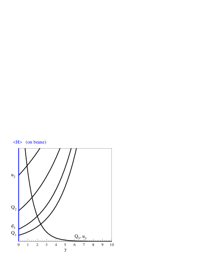
Figure 8: This figure, from [53], displays how the fermion mass hierarchy is achieved through localization of the chiral zero modes. The lighter quarks are localized away from $y=0$, while the third generation is peaked on the $y=0$ brane, so that it has a sizable overlap with the Higgs VEV.

4.4.1 Fermions in Warped Space

As shown in earlier parts of these lectures, the tools of warped spacetime could fix some of the phenomenological problems of flat extra dimensions, and we would now like to see whether we can replicate the standard model spectrum of fermions in AdS setups. The first complication is that we need to know the form of the covariant derivative acting on fermions in this curved spacetime.

To this end, we need an object constructed from the metric which lives in the spin 1/2 representation of the Lorentz group. In very rough terms, this object is the square root of the metric, $g$. In index notation, we write down the metric in terms of “vielbeins,” or in the case of 5 dimensions, a “fünfbein”:

$$g^{MN}=e_{a}^{M}\eta^{ab}e_{b}^{N}$$ (4.25)

The Dirac algebra is written in curved space in terms of the flat space Dirac matrices as

$$\Gamma^{M}=e^{M}_{a}\gamma^{a}$$ (4.26)

To write down the covariant derivative that can act on fermions, we use a spin connection, $w_{M}^{ab}$:

$$D_{M}=\partial_{M}+\frac{1}{2}w_{M}^{ab}\sigma_{ab},$$ (4.27)

where $\sigma_{ab}=\frac{1}{4}\gamma_{\left[a\right.}\gamma_{\left.b\right]}$. The spin connection can be expressed in terms of the fünfbeins as [60]

$$w_{M}^{ab}=\frac{1}{2}g^{RP}e^{\left[a\right.}_{R}\partial_{\left[M\right.}e^{\left.b\right]}_{\left.p\right]}+\frac{1}{4}g^{RP}g^{TS}e^{\left[a\right.}_{R}e^{\left.b\right]}_{T}\partial_{\left[S\right.}e^{c}_{\left.P\right]}e^{d}_{M}\eta_{cd}.$$ (4.28)

When the background geometry is given by AdS space, the metric (in conformal coordinates) is given by

$$ds^{2}=\left(\frac{R}{z}\right)^{2}\left(dx_{\mu}dx_{\nu}\eta^{\mu\nu}-dz^{2}\right).$$ (4.29)

One can show that $e^{a}_{M}=\left(\frac{R}{z}\right)\delta^{a}_{M}$, $D_{\mu}\psi=\left(\partial_{\mu}+\gamma_{\mu}\gamma_{5}\frac{1}{4z}\right)\psi$, and $D_{5}\psi=\partial_{5}\psi$. Proving that the spin connection terms cancel each other in this manner is left as an exercise for the reader.

Written in terms of the two component Weyl spinors, the AdS action will be

$$S=\int d^{5}x\left(\frac{R}{z}\right)^{4}\left(-i\bar{\chi}\bar{\sigma}^{\mu}\partial_{\mu}\chi-i\psi\sigma^{\mu}\partial_{\mu}\bar{\psi}+{\textstyle\frac{1}{2}}(\psi\overleftrightarrow{\partial_{5}}\chi-\bar{\chi}\overleftrightarrow{\partial_{5}}\bar{\psi})+\frac{c}{z}\left(\psi\chi+\bar{\chi}\bar{\psi}\right)\right),$$ (4.30)

where the coefficients $c=mR$, and $m$ is the bulk Dirac mass term for the 4-component Dirac spinor. In AdS space, the bulk equations of motion are [48]:

$$-i\bar{\sigma}^{\mu}\partial_{\mu}\chi-\partial_{5}\bar{\psi}+\frac{c+2}{z}\bar{\psi}=0,$$ (4.31)

$$-i\sigma^{\mu}\partial_{\mu}\bar{\psi}+\partial_{5}\chi+\frac{c-2}{z}\chi=0.$$ (4.32)

These have some subtle yet important features. The terms in the equations of motion that contain the bulk mass, $c$, are dependent on the extra dimensional coordinate, $z$. The $z$ dependent terms $2/z$ play an important role in determining the localization of any potential zero modes.

As before, we perform the KK decomposition. Everything from flat space carries over, except that the bulk equations of motion for the wave functions are different.

$$\chi=\sum_{n}g_{n}(z)\chi_{n}(x)\ \ \mathrm{and}\ \ \bar{\psi}=\sum_{n}f_{n}(z)\bar{\psi}_{n}(x),$$ (4.33)

where the 4D spinors $\chi_{n}$ and $\bar{\psi}_{n}$ satisfy the usual 4D Dirac equation with mass $m_{n}$:

$$-i\bar{\sigma}^{\mu}\partial_{\mu}\chi_{n}+m_{n}\bar{\psi}_{n}=0\ \ \mathrm{and}\ \ -i\sigma^{\mu}\partial_{\mu}\bar{\psi}_{n}+m_{n}\chi_{n}=0.$$ (4.34)

The bulk equations then become ordinary (coupled) differential equations of first order for the wavefunctions $f_{n}$ and $g_{n}$:

$$\displaystyle f^{\prime}_{n}+m_{n}g_{n}-\frac{c+2}{z}f_{n}=0,$$ (4.35)

$$\displaystyle g^{\prime}_{n}-m_{n}g_{n}+\frac{c-2}{z}g_{n}=0.$$ (4.36)

For a zero mode, if the boundary conditions were to allow its presence, these bulk equations are already decoupled and are thus easy to solve, leading to:

$$\displaystyle f_{0}=C_{0}\left(\frac{z}{R}\right)^{c+2},$$ (4.37)

$$\displaystyle g_{0}=A_{0}\left(\frac{z}{R}\right)^{2-c},$$ (4.38)

where $A_{0}$ and $C_{0}$ are two normalization constants of mass dimension $1/2$.

For the massive modes, just as with the flat space scenario, the first order differential equations can be uncoupled by combining them to get second order equations:

$$\displaystyle f^{\prime\prime}_{n}-{\textstyle\frac{4}{z}}f^{\prime}_{n}+(m_{n}^{2}-{\textstyle\frac{c^{2}-c-6}{z^{2}}})f_{n}=0,$$ (4.39)

$$\displaystyle g^{\prime\prime}_{n}-{\textstyle\frac{4}{z}}g^{\prime}_{n}+(m_{n}^{2}-{\textstyle\frac{c^{2}+c-6}{z^{2}}})g_{n}=0.$$ (4.40)

The solutions are now linear combinations of Bessel functions, as opposed to $\sin$ and $\cos$ functions:

$$\displaystyle g_{n}(z)=z^{\frac{5}{2}}\left(A_{n}J_{c+\frac{1}{2}}(m_{n}z)+B_{n}Y_{c+\frac{1}{2}}(m_{n}z)\right)$$ (4.41)

$$\displaystyle f_{n}(z)=z^{\frac{5}{2}}\left(C_{n}J_{c-\frac{1}{2}}(m_{n}z)+D_{n}Y_{c-\frac{1}{2}}(m_{n}z)\right).$$ (4.42)

The first order bulk equations of motion (4.35)-(4.36) further impose that

$$A_{n}=C_{n}\ \ \mathrm{and}\ \ B_{n}=D_{n}.$$ (4.43)

The remaining undetermined coefficients are determined by the boundary conditions, and the wave function normalization.

As in the flat space Kaplan-Tait model, the bulk mass determines the localization of the fermions. For instance, let us take

$$g_{0}(y)=A_{0}\left(\frac{z}{R}\right)^{2-c},\ \ f=0.$$ (4.44)

This solution corresponds to the boundary condition where $\psi|_{R,R^{\prime}}=0$. The coefficient $A_{0}$ is determined by the normalization condition

$$\int_{R}^{R^{\prime}}dz\left(\frac{R}{z}\right)^{5}\frac{z}{R}A_{0}^{2}\left(\frac{z}{R}\right)^{4-2c}=A_{0}^{2}\int^{R^{\prime}}_{R}\left(\frac{z}{R}\right)^{-2c}dz=1.$$ (4.45)

To understand from these equations where the fermions are localized, we study the behavior of this integral as we vary the limits of integration. For the boundary conditions that we are studying right now, if we send $R^{\prime}$ to infinity, we see that the integral remains convergent if $c>1/2$, and the fermion is then localized on the UV brane. If we send $R$ to zero, the integral is convergent if $c<1/2$, and the fermion is localized on the IR brane. The value of the Dirac mass determines whether the fermion is localized towards the UV or IR branes. We note that the opposite choice of boundary conditions that yields a zero mode ($\chi|_{R,R^{\prime}}=0$) results in a zero mode solution for $\psi$ with localization at the UV brane when $c<-1/2$, and at the IR brane when $c>-1/2$. The interesting feature in the warped case is that the localization transition occurs not when the bulk mass passes through zero, but at points where $|c|=1/2$. This is due to the curvature effects of the extra dimension.

4.5 Fermion Masses in the Higgsless Model

Recall the gauge symmetries of the Higgsless model in warped space shown in figure 6. The fermions in this model can not be completely localized on the UV or IR branes. If they were on the IR brane, the up-type and down-type quarks could not have any mass splitting as the theory is non-chiral at $z=R^{\prime}$, and if they were on the UV brane, the theory would be completely chiral, and the zero modes could not be lifted. The fermions must then live in the bulk, and feel the breakings of both branes. The quantum numbers of the fermions are given in Table 2.

	$SU(2)_{L}$	$SU(2)_{R}$	$U(1)_{B-L}$
$\left(\begin{array}[]{c}u\\ d\end{array}\right)_{L}$	$\Box$	$1$	$1/6$
$\left(\begin{array}[]{c}u\\ d\end{array}\right)_{R}$	$1$	$\Box$	$1/6$
$\left(\begin{array}[]{c}\nu\\ e\end{array}\right)_{L}$	$\Box$	$1$	$-1/2$
$\left(\begin{array}[]{c}\nu\\ e\end{array}\right)_{R}$	$1$	$\Box$	$-1/2$

Table 2: These are the quantum numbers of the bulk fermions under the bulk left-right symmetric Higgsless model.

The preliminary boundary conditions for the fermions that give the zero modes that we desire are given by

$$\left(\begin{array}[]{c}\chi_{u_{L}}\\ \bar{\psi}_{u_{L}}\\ \chi_{d_{L}}\\ \bar{\psi}_{d_{L}}\end{array}\right)\begin{array}[]{cc}+&+\\ -&-\\ +&+\\ -&-\end{array}\ \ \ \ \ \ \ \left(\begin{array}[]{c}\chi_{u_{R}}\\ \bar{\psi}_{u_{R}}\\ \chi_{d_{R}}\\ \bar{\psi}_{d_{R}}\end{array}\right)\begin{array}[]{cc}-&-\\ +&+\\ -&-\\ +&+\end{array}.$$ (4.46)

Where the $+$ and $-$ refer to whether we give those spinors Neumann or Dirichlet boundary conditions, respectively. These boundary conditions give massless chiral modes that match the fermion content of the standard model. However, the $u_{L}$, $d_{L}$, $u_{R}$, and $d_{R}$ are all massless at this stage, and we need to lift the zero modes to achieve the standard model mass spectrum. While simply giving certain boundary conditions for the fermions will enable us to lift these zero modes, in the following discussion, we talk about boundary operators, and the boundary conditions that these operators induce. There are some subtleties in dealing with boundary operators for fermions. These arise from the fact that the fields themselves are not always continuous in the presence of a boundary operator. This is due to the fact that the equations of motion for fermions are first order. The most straightforward approach is to enforce the boundary conditions that give the zero modes as shown in Eq. (4.46) on the real boundary at $z=R,R^{\prime}$ while the boundary operators are added on a fictitious brane a distance $\epsilon$ away from it. The distance between the fictitious brane and the physical one is taken to be $\epsilon$. The new boundary condition is then obtained by taking the distance $\epsilon$ to be small. This physical picture is quite helpful in understanding what the different boundary conditions will do.

To lift a doublet, we can give Dirac masses on the TeV brane which mix the $SU(2)_{L}$ and $SU(2)_{R}$ multiplets. This is possible because the theory on the IR brane is non-chiral. The boundary conditions that this Dirac mass gives on the IR brane are

$$\psi_{L}=-M_{D}R^{\prime}\psi_{R}\ \ \ \mathrm{and}\ \ \ \chi_{R}=M_{D}R^{\prime}\chi_{L}$$ (4.47)

At this stage, the up and down-type quarks, and the charged leptons and neutrinos are degenerate in mass. Mass splittings must be acquired on the UV brane, where the theory is chiral. For leptons and neutrinos, this can be accomplished simply by adding a Majorana mass for the neutrinos on the UV brane. The neutrino mass is suppressed by a type of see-saw mechanism while the lepton masses are unaffected.

As a complete example of the boundary operator prescription, we consider adding a Majorana mass for the $\nu_{R}$ on the UV brane. This is displayed in Figure 9. Going through the procedure described above, the new equation of motion is given by

$$-i\bar{\sigma}\partial_{\mu}\chi-\partial_{5}\bar{\psi}+\frac{c+2}{z}\bar{\psi}+\frac{MR^{2}}{z}\bar{\chi}\delta(z-R-\epsilon)=0$$ (4.48)

Integrating over the discontinuity, we obtain a jump condition for the spinor $\psi$:

$$\left[\psi\right]^{R+\epsilon}_{R}=MR\chi|_{R+\epsilon}.$$ (4.49)

With the condition that $\psi|_{R}=0$ and the small $\epsilon$ limit, we have a new effective boundary condition

$$\psi_{R+\epsilon}=MR\chi|_{R+\epsilon}$$ (4.50)

Figure 9: To give a physical picture to the boundary conditions used to lift a zero mode, a 4D majorana mass is added a slight distance from the boundary. The equations of motion are then solved, and the limit $\varepsilon\rightarrow 0$ is taken.

The general solutions to the bulk equations of motion are given by:

$$\chi_{L,R}=z^{5/2}\left[A_{L,R}J_{1/2+c_{L,R}}(mz)+B_{L,R}J_{-1/2-c_{L,R}}(mz)\right]$$

$$\psi_{L,R}=z^{5/2}\left[A_{L,R}J_{-1/2+c_{L,R}}(mz)-B_{L,R}J_{1/2-c_{L,R}}(mz)\right].$$ (4.51)

The coefficients are fixed by the boundary conditions given in Eqs. (4.47) and (4.50), and by imposing canonical normalizations for the KK modes in the 4D effective theory. The resulting mass spectrum for the lifted zero modes can be modified by changing the $c_{L,R}$ parameters, and the strengths of the boundary terms $M_{D}$, and $M$.

Accomplishing the quark splittings is slightly more complicated, and involves adding induced kinetic terms on the boundaries, or mixings with localized fermions. However, the splittings of the quarks can be achieved as well.

The final result is a spectrum which agrees with the standard model. It is possible to give the lighter fermions the right masses while all of them are strongly localized on the UV brane. This is ideal, since the distortion of the gauge boson wave functions towards the IR brane due to the warp factor will shift effective couplings to the fermion currents. The third generation of quarks poses a difficulty, however. To get a large enough mass for the top quark, the $(t,b)_{L}$ doublet must be localized towards the IR brane. This poses some difficulty for matching on to the measured value of the $Z\bar{b}b$ coupling [12]. This will be discussed further in the next lecture.

5 Electroweak Precision Observables For
General BSM and Extra Dimensional Theories

This lecture dealing with electroweak (EW) observables in extra dimensional theories will be split into two main lines of discussion. The first part of this lecture will be dealing with how to calculate electroweak precision observables from the effective Lagrangian point of view. This part of the lecture will be completely independent of extra dimensions and can be applied to any weakly coupled model of beyond the SM (BSM) physics. After this self contained introduction to EW observables in BSM physics we will move on to analyzing where generic corrections to SM EW observables come from in extra dimensional models. The focus will then be shifted to the particular cases of EW observables in RS models and the Higgsless models. The Higgsless models will be discussed in detail at the end of this section showing how they can both be ruled out from EW observables in their original incarnations; as well as how these models can be made consistent with EW fits when the original models are modified.

5.1 EW Observables and the Effective Lagrangian Point of View

There have already been a series of lectures on EW precision tests by James Wells during this TASI [61], however this lecture will give a slightly different point of view that we find very useful in practice. We will follow closely here the analysis done by Burgess et. al. in [62] but will attempt to give a mostly self contained presentation. There is a very generic program that can be applied to electroweak precision observables, and can be divided in the following way.

• First one needs to write down the most general effective Lagrangian allowed by the symmetries that are unbroken at the relevant energy scale (for instance for LEP I electroweak precision observables this would be $M_{Z}$).

• The second step after writing down the most general Lagrangian is to fix the coefficients for this effective Lagrangian for whatever model you are interested in analyzing.

• Once this work has been done the third and final step is to calculate the expressions for the desired observables in terms of the input parameters and the effective Lagrangian coefficients.

The desired observables for the particular model in question, $\mathcal{O}^{\mathrm{model}}$, are best usually to be expressed as $\mathcal{O}^{\mathrm{model}}=\mathcal{O}^{\mathrm{SM}}+\delta\mathcal{O}^{\mathrm{model}}$. The reason for expressing the observables for a particular model in this form is that the corrections $\delta\mathcal{O}^{\mathrm{model}}$ are usually small (or you better hope so if this is your model you are studying). One can then include the SM loop contributions into $\mathcal{O}^{\mathrm{SM}}$ and only deal with the tree-level $\delta\mathcal{O}^{\mathrm{model}}$. This is not always the case as there are cases of BSM physics where the tree-level contribution vanishes and loop level contributions must be calculated, for instance as in [63], however it can be successfully applied to a whole host of models. At this point once one has calculated the electroweak observables in the model of interest one simply needs to perform a fit to the experimental data and find the allowed regions of parameter space for a particular model.

At this point several comments are in order after laying out such a short and yet powerful program for testing new BSM physics possibilities. The first is that at no point in this program have we made any reference to “oblique” corrections or the S, T, U parameters [64] or the $\epsilon_{1}$, $\epsilon_{2}$, $\epsilon_{3}$ parameters [65]. Some students may have heard of these various parameterizations and associated their existence as the only calculations necessary for EW precision tests (EWPT). This is obviously not the case from the prescription we have laid out so far, yet there will be a large set of “universal” corrections that can be included in oblique corrections. The choice of parametrization is a matter of conventions and how you want to choose to express large sets of common corrections. For those who want more information on the common parameterizations we refer the reader to some original papers as well as useful reviews [61, 64, 65, 67, 66, 68, 69, 70].

We will begin now with taking the Lagrangian at the energy scale of the Z mass, $m_{Z}$, with the top quark and the Higgs integrated out along with any other BSM particles as well. The general form of the gauge boson Lagrangian will be

$$\mathcal{L}_{eff}=\mathcal{L}_{SM}(\tilde{e}_{i})+\hat{\mathcal{L}}_{new},$$ (5.1)

where $\mathcal{L}_{SM}(\tilde{e}_{i})$ is the ordinary SM Lagrangian with SM loop effects taken into account. The couplings of SM Lagrangian $\tilde{e}_{i}$ do not take their usual numerical values, because the new physics can contribute and has not been included. For example $\frac{\tilde{e}^{2}}{4\pi}=\frac{1}{128}$ will not necessarily hold due to the effects of $\mathcal{L}_{new}$ which must be taken into account. The form of $\mathcal{L}_{new}$ for the gauge boson sector up to dimension $4$ is

$$\hat{\mathcal{L}}_{new} = -\frac{A}{4}\hat{F}_{\mu\nu}\hat{F}^{\mu\nu}-\frac{B}{2}\hat{W}_{\mu\nu}\hat{W}^{\mu\nu}-\frac{C}{4}\hat{Z}_{\mu\nu}\hat{Z}^{\mu\nu}+\frac{G}{2}\hat{F}_{\mu\nu}\hat{Z}^{\mu\nu}$$ (5.2)

$$-w\tilde{m_{W}}^{2}\hat{W}_{\mu}^{+}\hat{W}^{\mu\,-}-\frac{z}{2}\tilde{m_{Z}}^{2}\hat{Z}_{\mu}\hat{Z}^{\mu}.$$

The reason the gauge fields $\hat{A}$,$\hat{W}$ and $\hat{Z}$ are hatted is because these are not canonically normalized fields. There was no trick to the procedure of what to write down in (5.2), we simply wrote down all dimension $\leq 4$ terms that are allowed by the remaining symmetries of the theory. $\hat{F}_{\mu\nu}$ and $\hat{Z}_{\mu\nu}$ are the usual Abelian field strengths, while the unbroken $U(1)_{EM}$ forces

$$\hat{W}_{\mu\nu}=D_{\mu}\hat{W}_{\nu}-D_{\nu}\hat{W}_{\mu}$$ (5.3)

where

$$D_{\mu}\hat{W}_{\nu}=\partial_{\mu}\hat{W}_{\nu}+i\tilde{e}A_{\nu}\hat{W}_{\mu}.$$ (5.4)

Let us assume for now that the rest of the SM Lagrangian in the gauge sector is unchanged, that is

$$\mathcal{L}_{EM} = -\tilde{e}\sum_{i}\bar{f}_{i}\gamma^{\mu}Q_{i}f_{i}\hat{A}_{\mu},$$

$$\mathcal{L}_{CC} = -\frac{\tilde{e}}{\tilde{s}_{W}\sqrt{2}}\sum_{ij}\tilde{V}_{ij}\bar{f}_{i}\gamma^{\mu}P_{L}f_{j}\hat{W}_{\mu}^{+}+\mathrm{c.c},$$

$$\mathcal{L}_{NC} = -\frac{\tilde{e}}{\tilde{s}_{W}\tilde{c}_{W}}\sum_{i}\bar{f}_{i}\gamma^{\mu}\left[T_{3i}P_{L}-Q_{i}\tilde{s}_{W}^{2}\right]f_{i}\hat{Z}_{\mu}.$$ (5.5)

If (5.1) holds we have $6$ parameters $A,B,C,G,w$, and $z$ however not all of them are physically observable. The reason for this is that field redefinitions of $W_{\mu}^{a},$ $B_{\mu}$ and the Higgs scalar $\phi$ can absorb $3$ of the six parameters. Therefore in the end only $3$ combinations of these parameters will appear in observables. Conventionally these three physical combinations are called the familiar $S,T,$ and $U$ parameters, which can be defined in terms of the parameters in (5.2) as

$$\alpha S = 4s_{W}^{2}c_{W}^{2}(A-C-\frac{c_{W}^{2}-s_{W}^{2}}{c_{W}s_{W}}G),$$

$$\alpha T = w-z,$$

$$\alpha U = 4s_{W}^{4}(A-\frac{B}{s_{W}^{2}}+\frac{c_{W}^{2}}{s_{W}^{2}}C-\frac{2c_{W}}{s_{W}}G)$$ (5.6)

Let us now begin to take into account the effect of the new physics by rescaling the fields to get canonically normalized gauge kinetic terms. Assuming the parameters $A,B,C,G,w,$ and $z$ are small we can go to canonically normalized kinetic terms with the following rescaling

$$\hat{A}_{\mu} = (1-\frac{A}{2})A_{\mu}+GZ_{\mu}$$

$$\hat{W}_{\mu} = (1-\frac{B}{2})W_{\mu}$$

$$\hat{Z}_{\mu} = (1-\frac{C}{2})Z_{\mu}.$$ (5.7)

This rescaling will bring the Lagrangian into the form

$$\mathcal{L}_{eff} = -\frac{1}{4}F_{\mu\nu}F^{\mu\nu}-\frac{1}{2}W_{\mu\nu}W^{\mu\nu}-\frac{1}{4}Z_{\mu\nu}Z^{\mu\nu}-(1+w-B)\tilde{m_{W}}^{2}W_{\mu}^{+}W^{\mu\,-}$$ (5.8)

$$-\frac{1}{2}(1+z-C)\tilde{m_{Z}}^{2}Z_{\mu}Z^{\mu}-\tilde{e}(1-\frac{A}{2})\sum_{i}\bar{f}_{i}\gamma^{\mu}Q_{i}f_{i}A_{\mu}$$

$$-\frac{\tilde{e}}{\tilde{s}_{W}\sqrt{2}}(1-\frac{B}{2})\sum_{ij}\tilde{V}_{ij}\bar{f}_{i}\gamma^{\mu}P_{L}f_{j}W_{\mu}^{+}+\mathrm{c.c}$$

$$-\frac{\tilde{e}}{\tilde{s}_{W}\tilde{c}_{W}}(1-\frac{C}{2})\sum_{i}\bar{f}_{i}\gamma^{\mu}\left[T_{3i}P_{L}-Q_{i}\tilde{s}_{W}^{2}+Q_{i}\tilde{s}_{W}\tilde{c}_{W}G\right]f_{i}Z_{\mu}.$$

The Lagrangian (5.8) depends on $3$ input parameters $\tilde{e},\tilde{s}_{W},$ and $\tilde{m}_{Z}$ (neglecting the CKM elements). However we would like to trade these input parameters for well measured quantities $\alpha,M_{z},G_{F}$ that take on their usual SM values. This will give us a relationship between the tilded parameters $\tilde{e},\tilde{s}_{W},\tilde{m}_{Z},$ and the measured observables $\alpha,M_{z},G_{F}$, which can be further used to express any other observables in terms of.

Starting with a general model as we have expressed so far, from (5.8) we have the relationship

$$4\pi\alpha=\tilde{e}^{2}(1-A).$$ (5.9)

In the SM this relationship takes the form $4\pi\alpha=e^{2}$, thus equating the two will lead us to a relationship between $\tilde{e}$ and $e$,

$$\tilde{e}=e\left(1+\frac{A}{2}\right).$$ (5.10)

Similarly defining

$$M_{Z}^{2}=\tilde{m}_{Z}^{2}(1+z-C)$$ (5.11)

allows us to write the obvious relationship

$$\tilde{m}_{z}^{2}=M_{z}^{2}(1-z+C).$$ (5.12)

We next turn our attention to $G_{F}$, Fermi’s constant, which is measured via $\mu$-decay. The relevant diagram is shown in Figure 10. Integrating out the W boson generates an effective four fermion operator whose dimensionful coupling constant is given by $G_{F}$. In the SM the expression defining $G_{F}$ is

$$\frac{G_{F}}{\sqrt{2}}=\frac{e^{2}}{8s_{W}^{2}c_{W}^{2}m_{Z}^{2}}.$$ (5.13)

There will be two effects that alter this relationship from the introduction of the new operators BSM. The first is the modified charged current interactions in (5.8) and the second will be the shift in the W propagator which comes from a shift in the pole mass which can be read off from (5.8) as well.

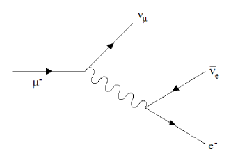
Figure 10: The process in the SM which contributes to $G_{F}$.

With these modifications from the effective Lagrangian we have the relation

$$\frac{G_{F}}{\sqrt{2}}=\frac{\tilde{e}^{2}(1-B)}{8\tilde{s}_{W}^{2}\tilde{c}_{W}^{2}\tilde{m}_{Z}^{2}(1+w-B)}\approx\frac{\tilde{e}^{2}(1-w)}{8\tilde{s}_{W}^{2}\tilde{c}_{W}^{2}\tilde{m}_{Z}^{2}}.$$ (5.14)

¿From this relationship and taking (5.13) as the definition of $s_{W}$ we can express $\tilde{s}_{W}^{2}$ as

$$\tilde{s}_{W}^{2}=s_{W}^{2}\left[1+\frac{c_{W}^{2}}{c_{W}^{2}-s_{W}^{2}}(A-C-w+z)\right].$$ (5.15)

We have now fixed part of the Lagrangian based on our chosen input parameters and by construction

$$\mathcal{L}_{Z} = -\frac{1}{2}M_{Z}^{2}Z_{\mu}Z^{\mu}$$

$$\mathcal{L}_{EM} = -e\sum_{i}\bar{f}_{i}\gamma^{\mu}Q_{i}f_{i}A_{\mu}.$$ (5.16)

However now we can express other observables in terms of our chosen input observables and find the predictions for the effects of the new physics. For instance the term in the Lagrangian governing the mass of the W was of the form

$$\mathcal{L}_{W}=-(1+w-B)\tilde{m}_{W}^{2}W_{\mu}^{+}W^{\mu-}=-(1+w-B)\tilde{c}_{W}^{2}\tilde{m}_{Z}^{2}W_{\mu}^{+}W^{\mu-}$$ (5.17)

where we have used the relationship $\tilde{m}_{w}=\tilde{m}_{z}\tilde{c}_{W}$ since these refer to the tilded (SM only) parameters which continue to take their natural relations. We have previously fixed the relationship of the tilded parameters to the input observables in (5.15) and (5.12) therefore we can re-express (5.17) as

$$\mathcal{L}_{W} = -(1+w-B)(1-z+C)\left[1-\frac{s_{W}^{2}}{c_{W}^{2}-s_{W}^{2}}(A-C-w+z)\right]M_{Z}^{2}c_{W}^{2}W_{\mu}^{+}W^{\mu-}$$ (5.18)

$$= -M_{Z}^{2}c_{W}^{2}\left[1-B+C+w-z-\frac{s_{W}^{2}}{c_{W}^{2}-s_{W}^{2}}(A-C-w+z)\right]W_{\mu}^{+}W^{\mu-}$$

If we now change to the S,T,U parametrization given in (5.1) then the prediction for the physical mass of the W as a function of the new physics is given by

$$(M_{W}^{2})_{phys}=(M_{W}^{2})_{SM}\left[1-\frac{\alpha S}{2(c_{W}^{2}-s_{W}^{2})}+\frac{c_{W}^{2}\alpha T}{c_{W}^{2}-s_{W}^{2}}+\frac{\alpha U}{4s_{W}^{2}}\right].$$ (5.19)

We can also analyze how other sectors of the Lagrangian are changed by our choice of input parameters and what the effects are for other observables. In the charged current sector the Lagrangian now takes the form

$$\mathcal{L}_{CC}=-\frac{e}{\sqrt{2}s_{W}}\left(1+\frac{1}{2}\left[A-B-\frac{c_{w}^{2}}{c_{W}^{2}-s_{W}^{2}}\left(A-C-w+z\right)\right]\right)\sum_{ij}V_{ij}\bar{f}_{i}\gamma^{\mu}P_{L}f_{j}W^{\mu+}+h.c.,$$ (5.20)

which can be rewritten with the help of $S,T,$ and $U$ as

$$\mathcal{L}_{CC}=-\frac{e}{\sqrt{2}s_{W}}\left(1-\frac{\alpha S}{4(c_{W}^{2}-s_{W}^{2})}+\frac{c_{W}^{2}\alpha T}{2(c_{W}^{2}-s_{W}^{2})}+\frac{\alpha U}{8s_{W}^{2}}\right)\sum_{ij}V_{ij}\bar{f}_{i}\gamma^{\mu}P_{L}f_{j}W^{\mu+}+h.c.$$ (5.21)

This now allows us to define a shifted coupling for charged current interactions as $h_{ij}\equiv h_{ij}^{SM}+\delta h_{ij}$, where $h_{ij}^{SM}=V_{ij}$ and the shift from new physics is

$$\delta h_{ij}=V_{ij}\left(-\frac{\alpha S}{4(c_{W}^{2}-s_{W}^{2})}+\frac{c_{W}^{2}\alpha T}{2(c_{W}^{2}-s_{W}^{2})}+\frac{\alpha U}{8s_{W}^{2}}\right)$$ (5.22)

which can be read off from (5.21). The neutral current sector is also changed to the form

$$\mathcal{L}_{NC}=-\frac{e}{s_{W}c_{W}}(1+\frac{\alpha T}{2})\sum_{i}\bar{f}_{i}\gamma^{\mu}\left[T_{3i}P_{L}-Q_{i}\left(s_{W}^{2}+\frac{\alpha S}{4(c_{W}^{2}-s_{W}^{2})}-\frac{c_{W}^{2}s_{W}^{2}\alpha T}{c_{W}^{2}-s_{W}^{2}}\right)\right]f_{i}Z_{\mu}.$$

With this form of the neutral current we can define the couplings $g_{L}\equiv g_{L}^{SM}+\delta g_{L}$ and $g_{R}\equiv g_{R}^{SM}+\delta g_{R}$ analogously to the previously defined $h_{ij}$, where

$$g_{L}^{SM} = T_{3i}-Q_{i}s_{W}^{2},$$

$$g_{R}^{SM} = -Q_{i}s_{W}^{2},$$

$$\mathrm{and}$$

$$\delta g_{iL,R} = \frac{\alpha T}{2}g_{iL,R}^{SM}-Q_{i}\left(\frac{\alpha S}{4(c_{W}^{2}-s_{W}^{2})}-\frac{c_{W}^{2}s_{W}^{2}\alpha T}{c_{W}^{2}-s_{W}^{2}}\right).$$ (5.24)

With these definitions we can tackle other observables such as the left right asymmetry at the $Z$-pole

$$A_{LR}=\frac{\Gamma(Z\rightarrow f_{L}\bar{f}_{L})-\Gamma(Z\rightarrow f_{R}\bar{f}_{R})}{\Gamma(Z\rightarrow f_{L}\bar{f}_{L})+\Gamma(Z\rightarrow f_{R}\bar{f}_{R})}.$$ (5.25)

The left-right asymmetry can be rewritten in terms of the neutral current couplings defined in (5.1) as

$$A_{LR} = \frac{g_{eL}^{2}-g_{eR}^{2}}{g_{eL}^{2}+g_{eR}^{2}}=A_{LR}^{SM}+\frac{4g_{eL}^{SM}g_{eR}^{SM}}{(g_{eL}^{SM^{2}}+g_{eR}^{SM^{2}})^{2}}(g_{eR}^{SM}\delta g_{eL}-g_{eL}^{SM}\delta g_{eR})$$ (5.26)

$$= A_{LR}^{SM}+\frac{4g_{eL}^{SM}g_{eR}^{SM}}{(g_{eL}^{SM^{2}}+g_{eR}^{SM^{2}})^{2}}(g_{eR}^{SM}-g_{eL}^{SM})\left(\frac{\alpha S}{4(c_{W}^{2}-s_{W}^{2})}-\frac{c_{W}^{2}s_{W}^{2}\alpha T}{c_{W}^{2}-s_{W}^{2}}\right)$$

This program can be carried out for all other relevant observables at the Z-pole and similarly one will get expressions that depend only upon the oblique parameters $S,T,$ and $U$. This conclusion should be expected if we recall the form of the “new” physics BSM that we introduced in (5.2). All corrections that we assumed in (5.2) appeared in the gauge boson sector only. Sometimes this will be the case for a given model, sometimes it won’t. The most common exceptions to new physics appearing only obliquely are:

• exchange of heavy gauge bosons (KK modes!) gives an additional contribution to $\mu$ decay as well as additional four fermion operators

• mixing of heavy and light gauge bosons could give a non-oblique contribution to the shift of $Zf\bar{f}$, $Wf_{i}f_{j}$ couplings

• non universal fermion wave functions in extra dimensions can also lead to the shift of $Zf\bar{f}$, $Wf_{i}f_{j}$ couplings

while all of these have examples in extra dimensions there are analogues in four dimensional models as well. To account for non-oblique corrections the program is no different in practice than the one we have just discussed, the only difference being the form of the effective Lagrangian (5.2). Instead of only including new operators in the gauge sector alone one could include shifts in other sectors of the model up to whatever dimension of operator was desired for accuracy. This program has been carried out in [62] up to and including dimension five operators and we refer the interested reader there for more details. Of course including all operators up to dimension five will not necessarily yield all the interesting physics since new four fermion operators are dimension six. However, this process can be straightforwardly extended to include a more general effective Lagrangian up to dimension six. The interested reader may also find useful the extended (beyond S,T, and U) “universal” parametrization by Barbieri et. al. [26] which can account for new four fermion operators.

Before we move on to investigating the specific effects of extra dimensions on EW precision observables we will further discuss oblique corrections in the Peskin-Takeuchi $S,T,$ and $U$ formalism since it is the most widely used. In the beginning of the effective Lagrangian approach (5.2) we started off with the parameters $A,B,C,G,w,$ and $z$ and then expressed these six parameters in terms of three physically measurable combinations $S,T,$ and $U$. The Peskin-Takeuchi formalism calls the parameters that we used in (5.2) by slightly different names,

$$\mathcal{L}_{new} = \frac{\Pi^{\prime}_{\gamma\gamma}(0)}{4}F_{\mu\nu}F^{\mu\nu}+\frac{\Pi^{\prime}_{WW}(0)}{2}W_{\mu\nu}W^{\mu\nu}+\frac{\Pi^{\prime}_{ZZ}(0)}{4}Z_{\mu\nu}Z^{\mu\nu}-\frac{\Pi^{\prime}_{\gamma Z}(0)}{2}F_{\mu\nu}Z^{\mu\nu}$$ (5.27)

$$+\Pi_{WW}(0)W_{\mu}^{+}W^{\mu\,-}+\frac{\Pi_{ZZ}(0)}{2}Z_{\mu}Z^{\mu}.$$

These are clearly the same parameters as what we used in (5.2), their alternative names come from the reference to the SM loop calculations in the Peskin-Takeuchi paper[64]. These parameters simply represent shifts in the propagators of the gauge boson. Using this language and defining

$$\Pi_{WW}(0)=g^{2}\Pi_{11}(0)\;\;\;\;\;\;\;\;\;\;\;\,\Pi^{\prime}_{WW}=g^{2}\Pi^{\prime}_{11}(0)$$

$$\Pi_{ZZ}(0)=(g^{2}+g^{{}^{\prime}2})\Pi_{33}(0)\;\;\Pi^{\prime}_{ZZ}(0)=(g^{2}+g^{{}^{\prime}2})(\Pi^{\prime}_{33}(0)-2s_{W}^{2}\Pi^{\prime}_{3Q}(0)+s_{W}^{4}\Pi^{\prime}_{QQ}(0))$$

$$\Pi^{\prime}_{\gamma\gamma}(0)=e^{2}\Pi^{\prime}_{QQ}(0)\;\;\;\;\;\;\;\;\;\;\;\;\,\Pi^{\prime}_{\gamma Z}(0)=gg^{\prime}(\Pi^{\prime}_{3Q}(0)-s_{W}^{2}\Pi^{\prime}_{QQ})$$ (5.28)

we can express the $S,T,$ and $U$ parameters in terms of these $\Pi$ as

$$S = 16\pi(\Pi^{\prime}_{33}(0)-\Pi^{\prime}_{3Q}(0))$$

$$T = \frac{4\pi}{s_{W}^{2}c_{W}^{2}M_{Z}^{2}}\left(\Pi_{11}(0)-\Pi_{33}(0)\right)$$

$$U = 16\pi(\Pi^{\prime}_{11}(0)-\Pi^{\prime}_{33}(0)).$$ (5.29)

We have now summarized a basic program that has been applied previously to a wide range of models from little Higgs models [71] to extra dimensional ones [72, 73] and we hope the reader can apply it to any model of their own interest.

5.2 Electroweak Precision and Extra Dimensions

With the formalism set up in Section 5.1 we may now move forward with showing in detail how we implement this for extra dimensional models. For our first example let us assume that the fermions will be localized at some given point. An important point we should make is that matching between $5D$ and $4D$ couplings is a convention. However when choosing your convention you want to make sure that your expressions are the simplest such that it minimizes the amount of work for you to do. For instance in a simple flat extra dimension the matching condition between $4D$ and $5D$ gauge couplings usually is

$$\frac{1}{g^{2}}=\frac{R}{g_{5}^{2}},\;\mathrm{and}\;\frac{1}{g^{{}^{\prime}2}}=\frac{R}{g_{5}^{{}^{\prime}2}}.$$ (5.30)

However if fermions are localized at one point, for instance $y=0$, the coupling of fermions to gauge bosons is not necessarily given by $g$ and $g^{\prime}$ but rather the $4D$ effective Lagrangian is of the form

$$\mathcal{L}\supset-\int\frac{1}{4}F_{\mu\nu}F^{\mu\nu}dy+g_{5}\bar{\psi}(0)\gamma_{\mu}\tilde{A}^{\mu}(0)\psi(0).$$ (5.31)

If we canonically normalize the gauge field $A_{\mu}$ this in turn shifts the interaction term to the form

$$\mathcal{L}_{int}=\frac{g_{5}}{\sqrt{R}}\bar{\psi}(0)\gamma_{\mu}\psi(0)A^{\mu}(0),$$ (5.32)

where the coupling will be given by $gA^{\mu}(0)$ if we match the gauge coupling as in (5.30). To ensure that all corrections in this example will be oblique requires that we need to pick the wave function at the location of the fermions to be $1$ (if we use this simple matching relationship). We note here that this is not always possible in the case that the fermions are localized at different points in the extra dimension. In this case the choice of the wave function will then tell us how to completely calculate the $S,T,$ and $U$ parameters. The effective wave function for the light modes will be

$$-\frac{1}{4}\int|\psi_{\gamma}(z)|^{2}dz\,F_{\mu\nu}F^{\mu\nu}-\frac{1}{2}\int|\psi_{z}(z)|^{2}dz\,Z_{\mu\nu}Z^{\mu\nu}-\frac{1}{2}\int|\psi_{W}(z)|^{2}dz\,W^{+}_{\mu\nu}W^{\mu\nu-}$$

$$+\int dz|\partial_{z}\psi_{W}|^{2}W^{+}_{\mu}W^{-\mu}+\int dz|\partial_{z}\psi_{Z}|^{2}Z_{\mu}Z^{\mu}+\mathrm{any}\,\mathrm{mass}\,\mathrm{from}\,\mathrm{Higgs}\,\mathrm{terms}$$ (5.33)

Equation (5.2) simply comes from the generic KK decomposition into $4D$ fields. Beginning with (after setting $A_{5}=0$ as previously discussed)

$$-\frac{1}{4}F_{MN}F^{MN}dz=-\frac{1}{4}\int F_{\mu\nu}F^{\mu\nu}dz-\frac{1}{2}\int(\partial_{5}A_{\mu})^{2}dz$$ (5.34)

and writing

$$A_{\mu}(x,z)=A_{\mu}^{0}(x)\psi_{A}^{0}(z)+\mathrm{KK\,modes}$$ (5.35)

we get contributions to the Lagrangian of the form

$$-\frac{1}{4}\int dz|\psi_{A}(z)|^{2}(\partial_{\mu}A^{0}_{\nu}(x)-\partial_{\nu}A_{\mu}^{0}(x))^{2}+\frac{1}{2}\int dz|\partial_{z}\psi_{A}(z)|^{2}A^{0}_{\mu}(x)A^{0\mu}(x).$$ (5.36)

As one can see from the last term in (5.36) a non-flat wave function $\psi^{0}_{A}(z)$ will contribute to a $4D$ mass term! With these, the expression for the various $\Pi$’s will be

$$g^{2}\Pi_{11}(0) = \int|\partial_{z}\psi_{W}(z)|^{2}dz$$

$$(g^{2}+g^{\prime 2})\Pi_{33}(0) = \int|\partial_{z}\psi_{Z}(z)|^{2}\ dz$$

$$1-g^{2}\Pi^{\prime}_{11}(0) = \int|\psi_{W}(z)|^{2}dz$$

$$1-(g^{2}+g^{\prime 2})\Pi^{\prime}_{33}(0) = \int|\psi_{Z}(z)|^{2}dz.$$ (5.37)

Now it is simply a matter of substituting these expressions into (5.1) to get the $S,T,$ and $U$ parameters.

For our next example we will look at the Randall-Sundrum model with all the fermions as well as the Higgs on the TeV brane, but with the gauge fields propagating in the bulk (this is not the most interesting case but probably the simplest to actually calculate[72]). Starting with the metric

$$ds^{2}=\frac{R}{z}(\eta_{\mu\nu}dx^{\mu}dx^{\nu}-dz^{2})$$ (5.38)

the form of the action will be

$$S_{5D}=\int d^{4}x\int_{R}^{R^{\prime}}dz\frac{R}{z}\left[-\frac{1}{2g_{5}^{2}}W_{MN}^{+}W^{MN-}-\frac{1}{4}\left(\frac{1}{g_{5}^{2}}+\frac{1}{g_{5}^{{}^{\prime}2}}\right)F_{MN}F^{MN}\right.$$

$$\left.-\frac{1}{4(g_{5}^{2}+g_{5}^{{}^{\prime}2})}Z_{MN}Z^{MN}+\frac{v^{2}}{4}\delta(z-R^{\prime})\frac{R}{z}W_{M}^{+}W^{M-}+\frac{v^{2}}{8}\delta(z-R^{\prime})\frac{R}{z}Z_{M}Z^{M}\right].$$ (5.39)

Solving for the wave functions, the expressions for the masses and wave functions of the $W$ and $Z$ are given by:

$$M_{W}^{2} = \frac{1}{4}\frac{g_{5}^{2}}{R\log{R^{\prime}/R}}\frac{R^{2}v^{2}}{R^{{}^{\prime}2}}\;\;\;\;\;\;\;\;\;M_{Z}^{2}=\frac{1}{4}\frac{g_{5}^{2}+g_{5}^{{}^{\prime}2}}{R\log{R^{\prime}/R}}\frac{R^{2}v^{2}}{R^{{}^{\prime}2}}$$

$$\psi_{W}^{(0)} = 1+\frac{M_{W}^{2}}{4}\left[z^{2}-R^{{}^{\prime}2}-2z^{2}\log{\frac{z}{R}}+2R^{{}^{\prime}2}\log{\frac{R^{\prime}}{R}}\right]$$

$$\psi_{Z}^{(0)} = \psi_{W}^{(0)}(M_{W}\rightarrow M_{Z}).$$ (5.40)

The normalization of the wave functions is chosen such that $\psi(R^{\prime})=1$ (where the fermions are assumed to be localized). We note that the Higgs being on the TeV brane will not allow a flat wave function for the $W$ and $Z$ in the bulk, which will give rise to non-zero $S,T,$ and $U$ parameters. Now we want to pick our matching conditions so we can find the relevant $\Pi$’s. We pick the simplest matching conditions

$$\frac{1}{g^{2}}=\frac{R\log{R^{\prime}/R}}{g_{5}^{2}}\;\;\;\;\;\;\;\;\frac{1}{g^{{}^{\prime}2}}=\frac{R\log{R^{\prime}/R}}{g_{5}^{{}^{\prime}2}}$$ (5.41)

which leads to the following expressions

$$\Pi^{\prime}_{11}(0)=\Pi^{\prime}_{33}(0) = -\frac{R^{2}}{R^{{}^{\prime}2}}v^{2}\frac{1}{8}\left(2R^{{}^{\prime}2}\log{R^{\prime}/R}-2R^{{}^{\prime}2}+\frac{R^{{}^{\prime}2}}{\log{R^{\prime}/R}}+\dots\right),$$ (5.42)

$$\Pi_{11}(0) = -\frac{M_{W}^{2}}{2}\Pi^{\prime}_{11}(0)\;\mathrm{and}\;\Pi_{33}(0)=-\frac{M_{Z}^{2}}{2}\Pi^{\prime}_{33}(0).$$ (5.43)

With these $\Pi$’s we can easily calculate the $S,T,$ and $U$ parameters as we did before and we find that

$$S=-4\pi f^{2}R^{{}^{\prime}2}\log{R^{\prime}/R},\;\;T=-\frac{\pi}{2c_{W}^{2}}f^{2}R^{{}^{\prime}2},\;\;U=0,$$ (5.44)

where $f$ is the SM Higgs VEV. We see from (5.44) that the contributions to $S$ and $T$ are quite sizeable. However in this case these are not the only corrections one must take into account. The KK modes of the gauge bosons localized on the TeV brane will generate large corrections to $4$-fermi operators, in particular $\mu$ decay and the definition of $G_{F}$. We can introduce a new parameter $V$ that measures the effect of the $4$-fermi operators on the definition of $G_{F}$. The effect of the ordinary $W$ boson does not give the full $G_{F}$ but we will call it $G_{F,W}$ which is given by

$$4\sqrt{2}G_{F,W}\equiv\frac{1}{\frac{f^{2}}{4}+\Pi_{11}(0)}.$$ (5.45)

The expression for the full $G_{F}$ defines the parameter $V$ as

$$G_{F}=G_{F,W}(1+V)$$ (5.46)

where $V$ captures the effect of the additional KK modes of the gauge bosons. If we recall from Figure 10, the process that defines $G_{F}$, we see that we need the full contribution to the $W$ propagator. This means that what we really need to do is calculate the full $5D$ zero momentum brane to brane propagator $\Delta_{W}(q=0,R^{\prime},R^{\prime})$. We can calculate $V$ in terms of $\Delta(0,R^{\prime},R^{\prime})$ and the W contribution (5.45) which gives

$$V=-\left(\Delta_{W}(0,R^{\prime},R^{\prime})+\frac{1}{\frac{f^{2}}{4}+\Pi_{11}(0)}\right)\left(\frac{f^{2}}{4}+\Pi_{11}(0)\right).$$ (5.47)

For the RS model the $W$ propagator will yield the result that

$$V=\frac{g^{2}}{8}f^{2}R^{{}^{\prime}2}\log{\frac{R^{\prime}}{R}}.$$ (5.48)

With the $S,T,$ and $U$ results (5.44) and the $V$ parameter (5.48) we can now express all SM Z-pole observables and find a bound on $R^{\prime}$. In this particular example one finds that $\frac{1}{R^{\prime}}>11\;\mathrm{TeV}$[72]. Of course this is not the most interesting case since we would prefer to have the fermions in the bulk (mostly localized to the Planck brane). However even in this case there is still a strong constraint on the model from the $T$ parameter. The strong constraint from the $T$ parameter in the original RS models with the SM gauge symmetries are due to the absence of a custodial $SU(2)$ symmetry. The solution to this is to put another $SU(2)_{R}$ gauge symmetry in the bulk of RS that is broken on the Planck brane [17]. By the AdS/CFT correspondence this is equivalent to adding a global custodial symmetry to the RS model as discussed in Section 3.

5.3 Electroweak Precision and Higgsless Models

We have seen from the previous Section 5.2 that to leading order in $\log{R^{\prime}/R}$ that $S=T=0$. However the first correction to the oblique parameters is $\mathcal{O}(\frac{1}{\log{R^{\prime}/R}}),$ which is relatively large and one must check whether this is compatible with experimental results. We first analyze the Higgsless model discussed in Section 3 with the addition of Planck brane kinetic terms

$$\frac{r}{4}W_{\mu\nu}^{L\,\,2}+\frac{r^{\prime}}{4}\frac{1}{g_{5R}^{2}+\tilde{g}_{5}^{2}}(g_{5L}B_{\mu\nu}+\tilde{g}_{5}W_{\mu\nu}^{R3})^{2}$$ (5.49)

and TeV brane kinetic terms

$$-\frac{R^{\prime}}{R}\left[\frac{\tau^{\prime}}{4}B_{\mu\nu}^{2}+\frac{\tau}{4}\frac{1}{g_{5R}^{2}+g_{5L}^{2}}(g_{5L}W^{L}_{\mu\nu}+g_{5L}W_{\mu\nu}^{R})^{2}\right].$$ (5.50)

We perform the matching calculation and carry out the program that we have been discussing and find the following approximate expressions for $S$ and $T$ to leading order in $\tau$,

$$S \approx \frac{6\pi}{g^{2}\log{\frac{R^{\prime}}{R}}}\frac{2}{1+\frac{g_{5R}^{2}}{g_{5L}^{2}}}\frac{1}{1+\frac{r}{R\log{R^{\prime}/R}}}\left(1+\frac{4}{3}\frac{\tau}{R}\right)$$

$$T \approx 0.$$ (5.51)

However $M_{W}^{2}$ is given by

$$M_{W}^{2}\approx\frac{2}{1+\frac{g_{5R}^{2}}{g_{5L}^{2}}}\frac{1}{1+\frac{r}{R\log{R^{\prime}/R}}}\frac{1}{R^{{}^{\prime}2}\log{R^{\prime}/R}}\left(1-\frac{g_{5R}^{2}}{g_{5R}^{2}+g_{5L}^{2}}\frac{\tau}{r+R\log{R^{\prime}/R}}\right).$$ (5.52)

The experimental constraints from the oblique parameters are

$$S=-0.13\pm 0.10$$

$$T=-0.17\pm 0.11$$

$$U=0.22\pm 0.12$$ (5.53)

for a $117$ GeV Higgs with $1$ $\sigma$ error bars given[74]. However the values are also correlated in the usual S-T plot as shown in Figure 11.

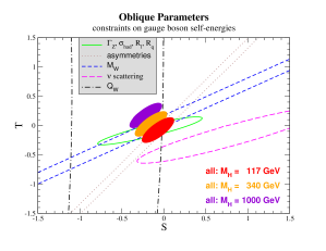
Figure 11: S-T Plot from PDG[74]

In the Higgsless models for $g_{5L}=g_{5R}$ and no induced kinetic terms the results for $S$ and $T$ are

$$S=1.15\;\;\;\;\;\;T=0$$ (5.54)

obviously completely excluding this form of the model[24].

This isn’t the end of the story since there is a solution [40] to the $S$ problem which has additional beneficial side-effects. It has been known for a long time in Randall-Sundrum (RS) models with a Higgs that the effective $S$ parameter is large and negative [72] if the fermions are localized on the TeV brane as originally proposed. When the fermions are localized on the Planck brane the contribution to $S$ is positive, and so for some intermediate localization the $S$ parameter vanishes, as first pointed out for RS models by Agashe et al.[17]. The reason for this is fairly simple. Since the $W$ and $Z$ wavefunctions are approximately flat, and the gauge KK mode wavefunctions are orthogonal to them, when the fermion wavefunctions are also approximately flat the overlap of a gauge KK mode with two fermions will approximately vanish. Since it is the coupling of the gauge KK modes to the fermions that induces a shift in the $S$ parameter, for approximately flat fermion wavefunctions the $S$ parameter must be small. Note that not only does reducing the coupling to gauge KK modes reduce the $S$ parameter, it also weakens the experimental constraints on the existence of light KK modes. This case of delocalized bulk fermions is not covered by the no-go theorem of [26], since there it was assumed that the fermions are localized on the Planck brane.

In order to quantify these statements, it is sufficient to consider a toy model where all the three families of fermions are massless and have a universal delocalized profile in the bulk. Before showing some numerical results, it is useful to understand the analytical behavior of $S$ in interesting limits. For fermions almost localized on the Planck brane, it is possible to expand the result for the $S$-parameter in powers of $(R/R^{\prime})^{2c_{L}-1}\ll 1$. The leading terms, also expanding in powers of $1/\log$, are:

$$S=\frac{6\pi}{g^{2}\,\log\frac{R^{\prime}}{R}}\left(1-\frac{4}{3}\frac{2c_{L}-1}{3-2c_{L}}\left(\frac{R}{R^{\prime}}\right)^{2c_{L}-1}\log\frac{R^{\prime}}{R}\right)~{},$$ (5.55)

and $U\approx T\approx 0$. The above formula is actually valid for $1/2<c_{L}<3/2$. For $c_{L}>3/2$ the corrections are of order $(R^{\prime}/R)^{2}$ and numerically negligible. As we can see, as soon as the fermion wave function starts leaking into the bulk, $S$ decreases.

Another interesting limit is when the profile is almost flat, $c_{L}\approx 1/2$. In this case, the leading contributions to $S$ are:

$$S=\frac{2\pi}{g^{2}\,\log\frac{R^{\prime}}{R}}\left(1+(2c_{L}-1)\,\log\frac{R^{\prime}}{R}+\mathcal{O}\left((2c_{L}-1)^{2}\right)\right)~{}.$$ (5.56)

In the flat limit $c_{L}=1/2$, $S$ is already suppressed by a factor of 3 with respect to the Planck brane localization case. Moreover, the leading terms cancel out for:

$$c_{L}=\frac{1}{2}-\frac{1}{2\,\log\frac{R^{\prime}}{R}}\approx 0.487~{}.$$ (5.57)

For $c_{L}<1/2$, $S$ becomes large and negative and, in the limit of TeV brane localized fermions ($c_{L}\ll 1/2$):

$$S=-\frac{16\pi}{g^{2}}\frac{1-2c_{L}}{5-2c_{L}}~{},$$ (5.58)

while, in the limit $c_{L}\rightarrow-\infty$:

$$T \rightarrow \frac{2\pi}{g^{2}\,\log\frac{R^{\prime}}{R}}(1+\tan^{2}\theta_{W})\approx 0.5~{},$$ (5.59)

$$U \rightarrow -\frac{8\pi}{g^{2}\,\log\frac{R^{\prime}}{R}}\frac{\tan^{2}\theta_{W}}{2+\tan^{2}\theta_{W}}\frac{1}{c_{L}}\approx 0~{}.$$ (5.60)

Figure 12: Plots of the oblique parameters as function of the bulk mass of the reference fermion. The values on the right correspond to localization on the Planck brane. $S$ vanishes for $c=0.487$.

In Fig. 12 we show the numerical results for the oblique parameters as function of $c_{L}$. We can see that, after vanishing for $c_{L}\approx 1/2$, $S$ becomes negative and large, while $T$ and $U$ remain smaller. With $R$ chosen to be the inverse Planck scale, the first KK resonance appears around $1.2$ TeV, but for larger values of $R$ this scale can be safely reduced down below a TeV. Such resonances will be weakly coupled to almost flat fermions and can easily avoid the strong bounds from direct searches at LEP or Tevatron. If we are imagining that the AdS space is a dual description of an approximate conformal field theory (CFT), then $1/R$ is the scale where the CFT is no longer approximately conformal and perhaps becomes asymptotically free. Thus it is quite reasonable that the scale $1/R$ would be much smaller than the Planck scale.

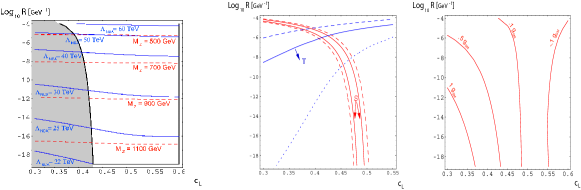
Figure 13: In the left plot we show the contour plots of $\Lambda_{\rm NDA}$ (solid blue lines) and $M_{Z^{(1)}}$ (dashed red lines) in the parameter space $c_{L}$–$R$. The shaded region is excluded by direct searches of light $Z^{\prime}$ at LEP. In the center, the contours of $S$ (red), for $|S|=0.25$ (solid) and $0.5$ (dashed) and $T$ (blue), for $|T|=0.1$ (dotted), $0.3$ (solid) and $0.5$ (dashed), as function of $c_{L}$ and $R$ are shown. On the right, contours for the generic suppression of fermion couplings to the first resonance with respect to the SM value can be seen. The region for $c_{L}$, allowed by $S$, is between $0.43\pm 0.5$, where the couplings are suppressed at least by a factor of 10.

In Fig. 13 we have plotted the value of the NDA scale (3.12) as well as the mass of the first resonance in the $(c_{L}-R)$ plane. Increasing $R$ also affects the oblique corrections. However, while it is always possible to reduce $S$ by delocalizing the fermions, $T$ increases and puts a limit on how far $R$ can be raised. One can also see from Fig. 13 that in the region where $|S|<0.25$, the coupling of the first resonance with the light fermions is generically suppressed to less than $10\%$ of the SM value. This means that the LEP bound of $2$ TeV for SM–like $Z^{\prime}$ is also decreased by a factor of 10 at least (the correction to the differential cross section is roughly proportional to $g^{2}/M_{Z^{\prime}}^{2}$). In the end, values of $R$ as large as $10^{-7}$ GeV^-1 are allowed, where the resonance masses are around $600$ GeV. So, even if, following the analysis of [34], we take into account a factor of roughly $1/4$ in the NDA scale, we see that the appearance of strong coupling regime can be delayed up to $10$ TeV. At the LHC it will be very difficult to probe $WW$ scattering above 3 TeV.

The major challenge facing Higgsless models is the incorporation of the third family of quarks. There is a tension [23, 17] in obtaining a large top quark mass without deviating from the observed bottom couplings with the $Z$. It can be seen in the following way. The top quark mass is proportional both to the Dirac mixing $M_{D}$ on the TeV brane and the overall scale of the extra dimension set by $1/R^{\prime}$. For $c_{L}\sim 0.5$ (or larger) it is in fact impossible to obtain a heavy enough top quark mass (at least for $g_{5R}=g_{5L}$). The reason is that for $M_{D}R^{\prime}\gg 1$ the light mode mass saturates at

$$m_{top}^{2}\sim\frac{2}{R^{\prime 2}\log\frac{R^{\prime}}{R}}\,,$$ (5.61)

which gives for this case $m_{top}\leq\sqrt{2}M_{W}$. Thus one needs to localize the top and the bottom quarks closer to the TeV brane. However, even in this case a sizable Dirac mass term on the TeV brane is needed to obtain a heavy enough top quark. The consequence of this mass term is the boundary condition for the bottom quarks

$$\chi_{bR}=M_{D}R^{\prime}\,\chi_{bL}.$$ (5.62)

This implies that if $M_{D}R^{\prime}\sim 1$ then the left handed bottom quark has a sizable component also living in an $SU(2)_{R}$ multiplet, which however has a coupling to the $Z$ that is different from the SM value. Thus there will be a large deviation in the $Zb_{L}\bar{b}_{L}$. Note, that the same deviation will not appear in the $Zb_{R}\bar{b}_{R}$ coupling, since the extra kinetic term introduced on the Planck brane to split top and bottom will imply that the right handed $b$ lives mostly in the induced fermion on the Planck brane which has the correct coupling to the $Z$.

The only way of getting around this problem would be to raise the value of $1/R^{\prime}$, and thus lower the necessary mixing on the TeV brane needed to obtain a heavy top quark. One way of raising the value of $1/R^{\prime}$ is by increasing the ratio $g_{5R}/g_{5L}$ (at the price of also making the gauge KK modes heavier and thus the theory more strongly coupled). Another possibility for rasing the value of $1/R^{\prime}$ is to separate the physics responsible for electroweak symmetry breaking from that responsible for the generation of the top mass. In technicolor models this is usually achieved by introducing a new strong interaction called topcolor. In the extra dimensional setup this would correspond to adding two separate AdS₅ bulks, which meet at the Planck brane [12]. One bulk would then be mostly responsible for electroweak symmetry breaking, the other for generating the top mass. The details of such models have been worked out in [12]. The main consequences of such models would be the necessary appearance of an isotriplet pseudo-Goldstone boson called the top-pion, and depending on the detailed implementation of the model there could also be a scalar particle (called the top-Higgs) appearing. This top-Higgs would however not be playing a major role in the unitarization of the gauge boson scattering amplitudes, but rather serve as the source for the top-mass only.

6 Conclusions

We have attempted to give an introduction to the uses of extra dimensions for electroweak physics. Clearly there are many other very interesting models in this field besides the higgsless theories, which we were not able to cover in these lectures. Here is a partial list of the most prominent models of new electroweak phenomenology from extra dimensions not covered here:

• The Randall-Sundrum model with custodial SU(2) [17], which can be thought of as the simplest implementation of the composite Higgs idea of Georgi and Kaplan.

• The hierarchy problem could also be possibly solved if the Higgs was secretly an extra dimensional component ($A_{5}$) of the gauge field. These theories are usually referred to as models with “gauge-higgs unification” [75] and were also the original inspirations for the little Higgs models of [76].

• Most recently [77], the above two approaches have been combined to get a model with gauge-higgs unification in warped space, with the $A_{5}$ component localized on the TeV brane. This way the Higgs would be a composite pseudo-Goldstone boson, explaining its lightness compared to the TeV scale. To date these are probably the most successful models of electroweak phenomenology from extra dimensions, which may even incorporate a successful unification of the gauge couplings [78].

We can only guess that there must be many other interesting models of the TeV scale that no one has thought of yet. We are all hoping that the guessing will end abruptly about 2-3 years from now, and at TASI 2009 we will already be lecturing about the definitive theory of electroweak symmetry breaking (and start a new guessing game of what lies beyond)…

References

- [1] N. Arkani-Hamed, S. Dimopoulos and G. R. Dvali, Phys. Lett. B 429, 263 (1998) [arXiv:hep-ph/9803315].
- [2] L. Randall and R. Sundrum, Phys. Rev. Lett. 83, 3370 (1999) [arXiv:hep-ph/9905221].
- [3] L. Randall and R. Sundrum, Phys. Rev. Lett. 83, 4690 (1999) [arXiv:hep-th/9906064].
- [4] C. Csáki, arXiv:hep-ph/0404096.
- [5] G. Kribs, lectures at TASI 2004.
- [6] R. Sundrum, arXiv:hep-th/0508134.
- [7] V. A. Rubakov, Phys. Usp. 44, 871 (2001) [Usp. Fiz. Nauk 171, 913 (2001)] [arXiv:hep-ph/0104152]; G. Gabadadze, arXiv:hep-ph/0308112. A. Perez-Lorenzana, arXiv:hep-ph/0503177.
- [8] A. Hebecker and J. March-Russell, Nucl. Phys. B 625, 128 (2002) [arXiv:hep-ph/0107039].
- [9] C. Csáki, C. Grojean, H. Murayama, L. Pilo and J. Terning, Phys. Rev. D 69, 055006 (2004) [arXiv:hep-ph/0305237].
- [10] G. R. Dvali, G. Gabadadze and M. Porrati, Phys. Lett. B 485, 208 (2000) [arXiv:hep-th/0005016]; G. R. Dvali and G. Gabadadze, Phys. Rev. D 63, 065007 (2001) [arXiv:hep-th/0008054]; G. R. Dvali, G. Gabadadze, M. Kolanovic and F. Nitti, Phys. Rev. D 64, 084004 (2001) [arXiv:hep-ph/0102216].
- [11] A. Muck, A. Pilaftsis and R. Ruckl, Phys. Rev. D 65, 085037 (2002) [arXiv:hep-ph/0110391].
- [12] G. Cacciapaglia, C. Csáki, C. Grojean, M. Reece and J. Terning, arXiv:hep-ph/0505001.
- [13] P. Candelas, G. T. Horowitz, A. Strominger and E. Witten, Nucl. Phys. B 258, 46 (1985); E. Witten, Nucl. Phys. B 258, 75 (1985); L. J. Dixon, J. A. Harvey, C. Vafa and E. Witten, Nucl. Phys. B 261, 678 (1985); E. Witten,
- [14] L. J. Hall and Y. Nomura, Phys. Rev. D 64, 055003 (2001) [arXiv:hep-ph/0103125].
- [15] Y. Kawamura, Prog. Theor. Phys. 105, 999 (2001) [arXiv:hep-ph/0012125]; G. Altarelli and F. Feruglio, Phys. Lett. B 511, 257 (2001) [arXiv:hep-ph/0102301].
- [16] R. S. Chivukula, D. A. Dicus and H. J. He, Phys. Lett. B 525, 175 (2002) hep-ph/0111016; R. S. Chivukula and H. J. He, Phys. Lett. B 532, 121 (2002) hep-ph/0201164; R. S. Chivukula, D. A. Dicus, H. J. He and S. Nandi, hep-ph/0302263; S. De Curtis, D. Dominici and J. R. Pelaez, Phys. Lett. B 554, 164 (2003) hep-ph/0211353; Phys. Rev. D 67, 076010 (2003) hep-ph/0301059; Y. Abe, N. Haba, Y. Higashide, K. Kobayashi and M. Matsunaga, Prog. Theor. Phys. 109, 831 (2003) hep-th/0302115.
- [17] K. Agashe, A. Delgado, M. J. May and R. Sundrum, JHEP 0308, 050 (2003) hep-ph/0308036.
- [18] C. Csáki, C. Grojean, L. Pilo and J. Terning, Phys. Rev. Lett. 92, 101802 (2004) hep-ph/0308038.
- [19] Y. Nomura, JHEP 0311, 050 (2003) hep-ph/0309189.
- [20] R. Barbieri, A. Pomarol and R. Rattazzi, Phys. Lett. B 591 (2004) 141 hep-ph/0310285.
- [21] C. Csáki, C. Grojean, J. Hubisz, Y. Shirman and J. Terning, Phys. Rev. D 70, 015012 (2004) hep-ph/0310355.
- [22] H. Davoudiasl, J. L. Hewett, B. Lillie and T. G. Rizzo, Phys. Rev. D 70, 015006 (2004) hep-ph/0312193.
- [23] G. Burdman and Y. Nomura, Phys. Rev. D 69, 115013 (2004) hep-ph/0312247.
- [24] G. Cacciapaglia, C. Csáki, C. Grojean and J. Terning, Phys. Rev. D 70, 075014 (2004) hep-ph/0401160.
- [25] H. Davoudiasl, J. L. Hewett, B. Lillie and T. G. Rizzo, JHEP 0405, 015 (2004) hep-ph/0403300; J. L. Hewett, B. Lillie and T. G. Rizzo, JHEP 0410, 014 (2004) hep-ph/0407059.
- [26] R. Barbieri, A. Pomarol, R. Rattazzi and A. Strumia, Nucl. Phys. B 703, 127 (2004) hep-ph/0405040.
- [27] R. Foadi, S. Gopalakrishna and C. Schmidt, JHEP 0403, 042 (2004) hep-ph/0312324; R. Casalbuoni, S. De Curtis and D. Dominici, Phys. Rev. D 70, 055010 (2004) hep-ph/0405188.
- [28] R. S. Chivukula, E. H. Simmons, H. J. He, M. Kurachi and M. Tanabashi, Phys. Rev. D 70, 075008 (2004) hep-ph/0406077; R. S. Chivukula, H. J. He, M. Kurachi, E. H. Simmons and M. Tanabashi, Phys. Lett. B 603, 210 (2004) hep-ph/0408262; R. Sekhar Chivukula, E. H. Simmons, H. J. He, M. Kurachi and M. Tanabashi, Phys. Rev. D 71, 035007 (2005) hep-ph/0410154.
- [29] H. Georgi, Phys. Rev. D 71, 015016 (2005) hep-ph/0408067.
- [30] H. Georgi, arXiv:hep-ph/0508014.
- [31] M. Perelstein, JHEP 0410, 010 (2004) hep-ph/0408072.
- [32] A. Birkedal, K. Matchev, and M. Perelstein, hep-ph/0412278.
- [33] C. Schwinn, hep-ph/0504240.
- [34] M. Papucci, hep-ph/0408058.
- [35] C. Schwinn, Phys. Rev. D 69, 116005 (2004) hep-ph/0402118; D. A. Dicus and H. J. He, hep-ph/0409131;
- [36] T. Ohl and C. Schwinn, Phys. Rev. D 70, 045019 (2004) hep-ph/0312263; Y. Abe, N. Haba, K. Hayakawa, Y. Matsumoto, M. Matsunaga and K. Miyachi, Prog. Theor. Phys. 113, 199 (2005) hep-th/0402146; A. Muck, L. Nilse, A. Pilaftsis and R. Ruckl, Phys. Rev. D 71, 066004 (2005) hep-ph/0411258.
- [37] J. Hirn and J. Stern, Eur. Phys. J. C 34, 447 (2004) hep-ph/0401032; JHEP 0409, 058 (2004) hep-ph/0403017.
- [38] N. Evans and P. Membry, hep-ph/0406285;
- [39] S. Gabriel, S. Nandi and G. Seidl, Phys. Lett. B 603, 74 (2004) hep-ph/0406020; T. Nagasawa and M. Sakamoto, Prog. Theor. Phys. 112, 629 (2004) hep-ph/0406024; C. D. Carone and J. M. Conroy, Phys. Rev. D 70, 075013 (2004) hep-ph/0407116; S. Chang, S. C. Park and J. Song, hep-ph/0502029; N. K. Tran, hep-th/0502205; J. Hirn and J. Stern, hep-ph/0504277.
- [40] G. Cacciapaglia, C. Csáki, C. Grojean and J. Terning, Phys. Rev. D 71, 035015 (2005) hep-ph/0409126.
- [41] R. Foadi, S. Gopalakrishna and C. Schmidt, Phys. Lett. B 606, 157 (2005) hep-ph/0409266;
- [42] R. S. Chivukula, E. H. Simmons, H. J. He, M. Kurachi and M. Tanabashi, hep-ph/0502162; R. Casalbuoni, S. De Curtis, D. Dolce and D. Dominici, hep-ph/0502209; R. S. Chivukula, H. J. He, M. Kurachi, E. H. Simmons and M. Tanabashi, hep-ph/0504114.
- [43] J. M. Maldacena, Adv. Theor. Math. Phys. 2, 231 (1998) [Int. J. Theor. Phys. 38, 1113 (1999)] hep-th/9711200.
- [44] N. Arkani-Hamed, M. Porrati, and L. Randall, JHEP 0108, 017 (2001) hep-th/0012148.
- [45] R. Rattazzi and A. Zaffaroni, JHEP 0104, 021 (2001) hep-th/0012248.
- [46] H. Davoudiasl, J. L. Hewett and T. G. Rizzo, Phys. Lett. B 473, 43 (2000) [arXiv:hep-ph/9911262]; Phys. Rev. D 63, 075004 (2001) [arXiv:hep-ph/0006041]; A. Pomarol, Phys. Lett. B 486, 153 (2000) [arXiv:hep-ph/9911294]; Phys. Rev. Lett. 85, 4004 (2000) [arXiv:hep-ph/0005293].
- [47] L. Randall and M. D. Schwartz, Phys. Rev. Lett. 88, 081801 (2002) [arXiv:hep-th/0108115].
- [48] Y. Grossman and M. Neubert, Phys. Lett. B 474, 361 (2000) [hep-ph/9912408].
- [49] T. Gherghetta and A. Pomarol, Nucl. Phys. B 586, 141 (2000) [hep-ph/0003129];
- [50] S. J. Huber and Q. Shafi, Phys. Lett. B 498, 256 (2001) [hep-ph/0010195]; Phys. Lett. B 512, 365 (2001) [hep-ph/0104293]; Phys. Lett. B 544, 295 (2002) [hep-ph/0205327].
- [51] Y. Nomura and D. R. Smith, Phys. Rev. D 68, 075003 (2003) [hep-ph/0305214].
- [52] S. J. Huber and Q. Shafi, hep-ph/0309252.
- [53] D. E. Kaplan and T. M. Tait, JHEP 0111, 051 (2001) [hep-ph/0110126].
- [54] I. Montvay, Relativisztikus kvantummechanika (Tankönyvkiadó, Budapest, 1977); You may also find the following link useful: http://szotar.sztaki.hu/magyar-angol . J. Polchinski, “String theory. Vol. 2: Superstring theory and beyond,”
- [55] J. Wess and J. Bagger, “Supersymmetry And Supergravity,” Princeton, USA: Univ. Pr. (1992) 259 p. ; J. A. Bagger, hep-ph/9604232.
- [56] D. B. Kaplan, Phys. Lett. B 288, 342 (1992) [hep-lat/9206013].
- [57] N. Arkani-Hamed and M. Schmaltz, Phys. Rev. D 61, 033005 (2000) [arXiv:hep-ph/9903417].
- [58] J. A. Bagger, F. Feruglio and F. Zwirner, Phys. Rev. Lett. 88, 101601 (2002) [hep-th/0107128];
- [59] J. Bagger, F. Feruglio and F. Zwirner, JHEP 0202, 010 (2002) [hep-th/0108010]; J. Bagger and M. Redi, hep-th/0310086.
- [60] R. Sundrum, Phys. Rev. D 59, 085009 (1999) [arXiv:hep-ph/9805471].
- [61] James Wells, TASI Notes 2004.
- [62] C. P. Burgess, S. Godfrey, H. Konig, D. London and I. Maksymyk, Phys. Rev. D 49, 6115 (1994) [arXiv:hep-ph/9312291].
- [63] J. Hubisz, P. Meade, A. Noble and M. Perelstein, arXiv:hep-ph/0506042.
- [64] M. E. Peskin and T. Takeuchi, Phys. Rev. Lett. 65, 964 (1990). M. E. Peskin and T. Takeuchi, Phys. Rev. D 46, 381 (1992).
- [65] G. Altarelli and R. Barbieri, Phys. Lett. B 253, 161 (1991). G. Altarelli, R. Barbieri and S. Jadach, Nucl. Phys. B 369, 3 (1992) [Erratum-ibid. B 376, 444 (1992)].
- [66] D. C. Kennedy and B. W. Lynn, Nucl. Phys. B 322, 1 (1989).
- [67] D. C. Kennedy, B. W. Lynn, C. J. C. Im and R. G. Stuart, Nucl. Phys. B 321, 83 (1989).
- [68] M. Golden and L. Randall, Nucl. Phys. B 361, 3 (1991).
- [69] B. Holdom and J. Terning, Phys. Lett. B 247, 88 (1990).
- [70] K. Matchev, arXiv:hep-ph/0402031.
- [71] C. Csaki, J. Hubisz, G. D. Kribs, P. Meade and J. Terning, Phys. Rev. D 67, 115002 (2003) [arXiv:hep-ph/0211124]. C. Csaki, J. Hubisz, G. D. Kribs, P. Meade and J. Terning, Phys. Rev. D 68, 035009 (2003) [arXiv:hep-ph/0303236].
- [72] C. Csaki, J. Erlich and J. Terning, Phys. Rev. D 66, 064021 (2002) [arXiv:hep-ph/0203034].
- [73] C. Csaki, J. Erlich, G. D. Kribs and J. Terning, Phys. Rev. D 66, 075008 (2002) [arXiv:hep-ph/0204109].
- [74] S. Eidelman et al. [Particle Data Group], Phys. Lett. B 592 (2004) 1. J. Erler and P. Langacker, arXiv:hep-ph/0407097.
- [75] N. S. Manton, Nucl. Phys. B 158, 141 (1979); I. Antoniadis, K. Benakli and M. Quiros, New J. Phys. 3, 20 (2001) hep-th/0108005; C. Csáki, C. Grojean and H. Murayama, Phys. Rev. D 67, 085012 (2003) hep-ph/0210133; C. A. Scrucca, M. Serone and L. Silvestrini, Nucl. Phys. B 669, 128 (2003) hep-ph/0304220; C. A. Scrucca, M. Serone, L. Silvestrini and A. Wulzer, JHEP 0402, 049 (2004) hep-th/0312267; K. Hasegawa, C. S. Lim and N. Maru, Phys. Lett. B 604, 133 (2004) hep-ph/0408028; N. Haba, K. Takenaga and T. Yamashita, hep-ph/0411250; Y. Hosotani and M. Mabe, hep-ph/0503020; G. Martinelli, M. Salvatori, C. A. Scrucca and L. Silvestrini, arXiv:hep-ph/0503179.
- [76] N. Arkani-Hamed, A. G. Cohen, E. Katz and A. E. Nelson, JHEP 0207, 034 (2002) hep-ph/0206021; N. Arkani-Hamed, A. G. Cohen, E. Katz, A. E. Nelson, T. Gregoire and J. G. Wacker, JHEP 0208, 021 (2002) [arXiv:hep-ph/0206020]; M. Schmaltz and D. Tucker-Smith, arXiv:hep-ph/0502182.
- [77] K. Agashe, R. Contino and A. Pomarol, Nucl. Phys. B 719, 165 (2005) [arXiv:hep-ph/0412089].
- [78] K. Agashe, R. Contino and R. Sundrum, arXiv:hep-ph/0502222.