Neutrinos in a left-right model with a horizontal symmetry

Abstract

We analyze the lepton sector of a Left-Right Model based on the gauge group $SU(2)_{L}\times SU(2)_{R}\times U(1)$, concentrating mainly on neutrino properties. Using the seesaw mechanism and a horizontal symmetry, we keep the right-handed symmetry breaking scale relatively low, while simultaneously satisfying phenomenological constraints on the light neutrino masses. We take the right-handed scale to be of order 10’s of TeV and perform a full numerical analysis of the model’s parameter space, subject to experimental constraints on neutrino masses and mixings. The numerical procedure yields results for the right-handed neutrino masses and mixings and the various CP-violating phases. We also discuss phenomenological applications of the model to neutrinoless double beta decay, lepton-flavor-violating decays (including decays such as $\tau\to 3\mu$) and leptogenesis.

I Introduction

The Standard Model (SM) of particle physics has thus far provided an incredibly accurate description of all observed experimental data. Nevertheless, the SM is widely regarded as being a low-energy effective theory, with a limited range of applicability and predictability. New interactions must arrive at the energy scale of several TeV in order to explain such features of the SM as the quark and lepton mass hierarchy.

An intriguing aspect of the SM is that its weak interaction sector represents the only known interaction that distinguishes between the right- and left-handed fermions. This aspect is addressed in a set of aesthetically-pleasing “left-right models” (LRMs) based on the gauge group $SU(2)_{L}\times SU(2)_{R}\times U(1)$, where the left- and right-handed fermion fields are treated symmetrically Pati and Salam (1974); Mohapatra and Pati (1975a, b); Senjanovic and Mohapatra (1975); Mohapatra et al. (1978); Senjanovic (1979); Duka et al. (2000). In such models, left-right symmetry is broken at some high scale, yielding a parity-violating Standard Model-like theory at low energies. In typical phenomenological studies of the LRM, the right-handed scale (i.e., the scale at which $SU(2)_{R}$ is broken) is assumed to be very high, of the order of $10^{10}$ GeV. Such a high energy scale would render direct experimental verification of a LR-motivated scenario impossible in the near future. By way of contrast, more moderate values for the right-handed scale – in the range 20-50 TeV, say – could have observable consequences at experiments in the near future Ball et al. (2000); Kiers et al. (2002). This is the energy range that we shall consider in this work.

Recently, there has been a renewed interest in the LRM, in particular, due to the discovery of neutrino oscillations and to major advances in experimental studies of CP-violation in the quark sector. Of interest to us in this work is that the LRM provides a natural process for the suppression of neutrino masses through the seesaw mechanism. LRMs also offer additional sources of CP violation, coming both from the right-handed Cabibbo-Kobayashi-Maskawa (CKM) and Maki-Nakagawa-Sakata (MNS) matrices as well as from the Higgs sector of the theory Kiers et al. (2005). The CP violation occuring in the leptonic sector of the model could in principle be of interest within the context of leptogenesis Fukugita and Yanagida (1986); Luty (1992); Buchmuller and Plumacher (1996); Hambye and Senjanovic (2004); Antusch and King (2004); Chen and Mahanthappa (2005); Atwood et al. (2005). It is important to emphasize that the phases in the left-handed MNS matrix are currently unconstrained.

As noted above, the LRM contains the natural possibility of implementing the seesaw mechanism for the generation of small neutrino masses. In the simplest version of the seesaw mechanism, only the SM-singlet right-handed neutrinos are initially allowed to obtain Majorana mass terms, resulting in the neutrino mass matrix

$${\cal M}=\left(\begin{array}[]{cc}0&M_{LR}\\ M_{LR}^{T}&M_{RR}\\ \end{array}\right)\;,$$ (3)

where $M_{RR}$ and $M_{LR}$ are Majorana and Dirac mass matrices, respectively, in flavour-space. This construction, with a block of “zeros” where the left-handed Majorana mass terms would go, leads to what is sometimes called the “Type I” seesaw mechanism. It can be generated in the LRM. An approximate block-diagonalization of Eq. (3), assuming that the elements in $M_{RR}$ are much larger than those in $M_{LR}$, leads to the standard seesaw expression for the light neutrino mass matrix, $M_{\nu}\simeq-M_{LR}M_{RR}^{-1}M_{LR}^{T}\equiv M_{\nu}^{I}$.

To implement the seesaw mechanism in the LRM, one introduces a right-handed Higgs triplet field, $\Delta_{R}$, into the theory. The field $\Delta_{R}$ serves a dual purpose – it breaks the left-right symmetry of the model at a high scale and it also couples to Majorana neutrino fields, giving rise to the right-handed Majorana mass matrix $M_{RR}$ required for the seesaw mechanism. $M_{RR}$ is proportional to the right-handed symmetry breaking scale, making it naturally large. Left-right symmetry also requires the existence of a left-handed Higgs triplet field, $\Delta_{L}$. The neutral components of the left- and right-handed triplet fields both generically obtain a vacuum expectation value (VEV) under spontaneous symmetry breaking, $\langle\delta^{0}_{L,R}\rangle=v_{L,R}e^{i\theta_{L,R}}/\sqrt{2}$. LRMs also typically contain a bidoublet field, $\phi$, with VEVs at the weak scale. The role played by $\phi$ is similar to that played by the usual Higgs doublet of the SM.

In contrast with the situation in the Type I seesaw mechanism, LRMs generically also contain a non-zero left-handed Majorana mass matrix for neutrinos, $M_{LL}$. This mass matrix is proportional to $v_{L}$ (the VEV associated with the left-handed Higgs triplet) and $v_{L}$ need not be zero. There is, in fact, a seesaw-like relation among the VEVs $v_{L}$ and $v_{R}$ in the LRM that arises due to terms in the Higgs potential that couple $\phi$, $\Delta_{L}$ and $\Delta_{R}$ ($\mbox{Tr}(\phi\Delta_{R}\phi^{\dagger}\Delta_{L}^{\dagger})$, for example). If all dimensionless coefficients in the Higgs potential are of order unity, one finds that $v_{L}\sim k^{2}/v_{R}$, where $k$ is a dimensionful quantity of order the weak scale Mohapatra and Senjanovic (1981); Deshpande et al. (1991); Kiers et al. (2005). The situation $v_{L}=0$ (and hence $M_{LL}=0$) can be obtained by dropping the offending terms from the Higgs potential, although attempts to disallow the terms using a symmetry meet with difficulties Deshpande et al. (1991). Inclusion of a non-zero matrix $M_{LL}^{\dagger}$ in the “zero” block of Eq. (3) (see Eq. (33) below) leads to the “Type II” seesaw mechanism Mohapatra and Senjanovic (1981); Mohapatra (2001), yielding the following approximate mass matrix for light neutrinos,

$$M_{\nu}\simeq M_{LL}^{\dagger}-M_{LR}M_{RR}^{-1}M_{LR}^{T}\equiv M_{\nu}^{II}+M_{\nu}^{I},$$ (4)

with $M_{LL}$ generically of order $v_{L}\sim k^{2}/v_{R}$ and $M_{RR}\sim v_{R}$. Experimentally, the terms in $M_{\nu}$ must be at most of order about 0.1 eV. If the largest terms in $M_{LR}$ are taken to be of order $m_{\tau}$, and if $M_{LL}$ does not undergo any further suppression, then the first term in Eq. (4) dominates and sets the minimum scale $v_{R}$ that is phenomenologically viable. Taking $k$ to be of order the weak scale we find that $v_{R}$ would need to be at least of order $10^{14}$ GeV in this case, ruling out any possibility of observing LR-induced effects at collider experiments. The analogous lower bound coming from the second term alone (Type I seesaw) is of order $10^{10}$ GeV if one assumes $M_{LR}\sim m_{\tau}$.

A few approaches have been suggested for reducing the right-handed scale $v_{R}$ while simultaneously satisfying phenomenological constraints within the context of Type II models. One approach is to suppress $M_{LL}$ by separating the parity and gauge symmetry breaking scales. For instance, one can introduce a pseudoscalar Higgs field $\eta$ that acquires a vacuum expectation value (thereby breaking parity) at a very high scale, while allowing the right-handed gauge symmetry to be broken at a much lower scale Chang et al. (1984); Chang and Mohapatra (1985) This approach could lead to interesting phenomenology. In such a model, $M_{LL}\sim k^{2}v_{R}/\langle\eta\rangle^{2}$, so that the left-handed Majorana mass terms could be of an acceptable size provided that $\langle\eta\rangle$ were sufficiently high.

Another promising approach for bringing $v_{R}$ down to a potentially observable scale is to introduce an extra $U(1)$ horizontal symmetry that is broken by a small parameter $\epsilon$ Froggatt and Nielsen (1979); Leurer et al. (1993); Khasanov and Perez (2002); Kiers et al. (2005). In this approach, each field in the model is assigned a charge under the horizontal symmetry. Yukawa couplings and the dimensionless coefficients in the Higgs potential are then suppressed by various powers of $\epsilon$, with the powers depending on combinations of charge assignments. In addition to providing a nice dynamical mechanism for producing the observed hierarchies in the charged lepton masses, this approach also allows for a significant reduction in the right-handed scale $v_{R}$. As shown in Refs. Khasanov and Perez (2002); Kiers et al. (2005), an appropriate choice of charge assignments leads to a suppression of $v_{L}$, thereby suppressing $M_{LL}$. There is a similar suppression of the Yukawa couplings involved in $M_{LR}$, the net effect of which is to loosen the stringent lower bounds on $v_{R}$.

In this work we perform an indepth numerical study of neutrinos in a left-right model that is supplemented by such a broken $U(1)$ horizontal symmetry. The goal of the paper is to determine the parameter space of the model already constrained by the neutrino mass and mixing measurements. We focus on the case in which the right-handed symmetry breaking scale is only “moderately” large (20-50 TeV). In the horizontal symmetry scheme, right-handed scales as low as 20 TeV can in fact lead to results consistent with neutrino phenomenology. The numerical procedure also yields results for the right-handed neutrino masses and mixings and the various CP-violating phases. Throughout this work we assume that there are three generations of light neutrinos and ignore the possibility of light sterile neutrinos. We also assume the “normal” ordering of neutrino masses, $m_{\nu_{1}}<m_{\nu_{2}}<m_{\nu_{3}}$.

The outline of the remainder of the paper is as follows. In Sec. II we describe the LRM and establish our notation. Section III contains our numerical results for the allowed parameter space of the model, as well as a discussion of some phenomenological applications such as lepton-flavor violating transitions and leptogenesis. We conclude with a brief discussion in Sec. IV. The Appendix contains approximate expressions for the right-handed neutrino masses and mixings as well as a particular case study.

II The Model

II.1 Mass and MNS matrices

The LRM is based on the gauge group $SU(2)_{L}\times SU(2)_{R}\times U(1)_{B-L}$. We will consider a minimal version of the model, whose Higgs sector contains a bidoublet Higgs boson field $\phi\sim(2,\overline{2},0)$ and two triplet Higgs boson fields $\Delta_{L}\sim(3,1,2)$ and $\Delta_{R}\sim(1,3,2)$. As noted in the Introduction, $\Delta_{R}$ is used to break the gauge symmetry down to $SU(2)_{L}\times U(1)_{Y}$ and $\phi$ is used to break it down to $U(1)_{\textrm{\scriptsize{em}}}$. The various Higgs boson fields may be parametrized as follows,

$$\phi=\left(\begin{array}[]{cc}\phi_{1}^{0}&\phi_{1}^{+}\\ \phi_{2}^{-}&\phi_{2}^{0}\\ \end{array}\right)\;,~{}~{}\Delta_{L,R}=\left(\begin{array}[]{cc}\delta^{+}_{L,R}/\sqrt{2}&\delta^{++}_{L,R}\\ \delta^{0}_{L,R}&-\delta^{+}_{L,R}/\sqrt{2}\\ \end{array}\right)\;.$$ (9)

The left- and right-handed lepton fields transform as doublets under $SU(2)_{L}$ and $SU(2)_{R}$, respectively, and are given by

$$\psi^{\prime}_{iL,R}=\left(\begin{array}[]{c}\nu^{\prime}_{iL,R}\\ e^{\prime}_{iL,R}\\ \end{array}\right)\;,$$ (12)

where $i$ is a generation index and where the primes denote that the fields are gauge eigenstates. In addition to the gauge symmetry, it is common to impose an extra left-right parity symmetry Deshpande et al. (1991), demanding invariance under

$$\psi^{\prime}_{iL}\leftrightarrow\psi^{\prime}_{iR},~{}~{}~{}\phi\leftrightarrow\phi^{\dagger},~{}~{}~{}\Delta_{L}\leftrightarrow\Delta_{R}.$$ (13)

The lepton Yukawa couplings that are consistent with the gauge and parity symmetries discussed above are Deshpande et al. (1991)

$$-{\mathcal{L}}_{\textrm{\scriptsize Yukawa}}=\overline{\psi}_{iL}^{\prime}\left(G_{ij}\phi+H_{ij}\widetilde{\phi}\right)\psi_{jR}^{\prime}+\frac{i}{2}F_{ij}\left(\psi^{\prime T}_{iL}C\tau_{2}\Delta_{L}\psi^{\prime}_{jL}+\psi^{\prime T}_{iR}C\tau_{2}\Delta_{R}\psi^{\prime}_{jR}\right)+\textrm{h.c.}\;,$$ (14)

where $\widetilde{\phi}=\tau_{2}\phi^{*}\tau_{2}$ and where $C=i\gamma^{2}\gamma^{0}$ is the charge conjugation matrix. In order to respect the parity symmetry in Eq. (13), the $3\times 3$ matrices $G$ and $H$ must be Hermitian. The matrix $F$ is complex, in general, but may be taken to be symmetric without any loss in generality.

Upon spontaneous symmetry breaking the Higgs boson fields acquire VEVs, which may be parametrized as

$$\langle\phi\rangle=\left(\begin{array}[]{cc}k_{1}/\sqrt{2}&0\\ 0&k_{2}e^{i\alpha}/\sqrt{2}\\ \end{array}\right),~{}~{}~{}\langle\Delta_{L}\rangle=\left(\begin{array}[]{cc}0&0\\ v_{L}e^{i\theta_{L}}/\sqrt{2}&0\\ \end{array}\right),~{}~{}~{}\langle\Delta_{R}\rangle=\left(\begin{array}[]{cc}0&0\\ v_{R}/\sqrt{2}&0\\ \end{array}\right),$$ (21)

with $k_{1,2}$ and $v_{L,R}$ real and positive. Gauge rotations have been used to eliminate possible phases associated with $k_{1}$ and $v_{R}$ Deshpande et al. (1991). Phenomenological constraints require that $v_{R}\gg k_{1},k_{2}\gg v_{L}$. In this case $k_{1}$ and $k_{2}$ satisfy the constraint Langacker and Uma Sankar (1989)

$$k_{1}^{2}+k_{2}^{2}\simeq\frac{4m_{W}^{2}}{g^{2}}\simeq(246.2~{}\textrm{GeV})^{2}\;.$$ (22)

Also, it is natural to assume $k_{2}/k_{1}\sim m_{b}/m_{t}$; in the numerical work below we shall set $k_{2}/k_{1}=3/181$ as in Ref. Kiers et al. (2002).

The VEVs in Eq. (21) lead to Dirac mass terms for the neutrinos and charged leptons,

$$-{\mathcal{L}}_{\textrm{\scriptsize Dirac}}=\frac{1}{\sqrt{2}}\;\overline{\nu^{\prime}_{L}}\left(Gk_{1}+Hk_{2}e^{-i\alpha}\right)\nu_{R}^{\prime}+\frac{1}{\sqrt{2}}\;\overline{e^{\prime}_{L}}\left(Gk_{2}e^{i\alpha}+Hk_{1}\right)e_{R}^{\prime}+\textrm{h.c.}\;,$$ (23)

as well as Majorana mass terms for the neutrinos,

$$-{\mathcal{L}}_{\textrm{\scriptsize Majorana}}=\frac{1}{2\sqrt{2}}\left(\overline{\nu_{L}^{\prime c}}Fv_{L}e^{i\theta_{L}}\nu^{\prime}_{L}+\overline{\nu_{R}^{\prime c}}Fv_{R}\nu^{\prime}_{R}\right)+\textrm{h.c.},$$ (24)

where $\nu_{L,R}^{\prime c}\equiv C\overline{\nu_{L,R}^{\prime}}^{T}$. The mass matrix for the charged leptons is thus

$$M_{\ell}=\frac{1}{\sqrt{2}}\left(Gk_{2}e^{i\alpha}+Hk_{1}\right)\;,$$ (25)

which may be diagonalized by a biunitary transformation

$$M_{\ell}^{\textrm{\scriptsize diag}}=V_{L}^{\ell\dagger}M_{\ell}V_{R}^{\ell}\;,$$ (26)

where the elements in $M_{\ell}^{\textrm{\scriptsize diag}}$ are real and positive.

Consideration of the neutrino mass matrix is slightly complicated by the fact that both Majorana and Dirac mass terms are present. Defining

$$\Psi_{\nu}^{\prime}=\left(\begin{array}[]{c}\nu_{L}^{\prime}\\ \nu_{R}^{\prime c}\\ \end{array}\right)$$ (29)

allows the neutrino mass terms in the Lagrangian to be written as

$$-{\mathcal{L}}_{m_{\nu}}=\frac{1}{2}\overline{\Psi_{\nu}^{\prime}}{\cal M}\Psi_{\nu}^{\prime c}+\textrm{h.c.},$$ (30)

where the Majorana and Dirac neutrino mass matrices have been incorporated into a single $6\times 6$ complex symmetric matrix

$${\cal M}=\left(\begin{array}[]{cc}M_{LL}^{\dagger}&M_{LR}\\ M_{LR}^{T}&M_{RR}\\ \end{array}\right)\;,$$ (33)

with

$$M_{LR}=\frac{1}{\sqrt{2}}\left(Gk_{1}+Hk_{2}e^{-i\alpha}\right)\;,~{}~{}~{}~{}~{}~{}M_{LL}=\frac{1}{\sqrt{2}}Fv_{L}e^{i\theta_{L}},~{}~{}~{}~{}~{}M_{RR}=\frac{1}{\sqrt{2}}Fv_{R}.$$ (34)

The $6\times 6$ neutrino mass matrix ${\cal M}$ may be approximately block diagonalized into a light, mostly left-handed block, $M_{\nu}$, and a heavy, mostly right-handed block, $M_{R}$,

$$\left(\begin{array}[]{cc}M_{\nu}&0\\ 0&M_{R}\\ \end{array}\right) \simeq \left(\begin{array}[]{cc}1&\xi^{\dagger}\\ -\xi&1\\ \end{array}\right)^{T}\left(\begin{array}[]{cc}M_{LL}^{\dagger}&M_{LR}\\ M_{LR}^{T}&M_{RR}\\ \end{array}\right)\left(\begin{array}[]{cc}1&\xi^{\dagger}\\ -\xi&1\\ \end{array}\right)$$ (43)

$$\simeq \left(\begin{array}[]{cc}M_{LL}^{\dagger}-M_{LR}M_{RR}^{-1}M_{LR}^{T}&0\\ 0&M_{RR}\\ \end{array}\right)$$ (46)

where $\xi=M_{RR}^{-1}M_{LR}^{T}$. The corrections to Eqs. (43) and (46) are suppressed by $\xi$ and may be neglected if $\left|\xi_{ij}\right|\ll 1$. (In our numerical work below, the magnitudes of the elements of $\xi$ are of order $10^{-5}$ or smaller, so the approximation is well-justified.) The above result for $M_{\nu}$ was quoted in Eq. (4) and is the general expression for the Type II seesaw mechanism. While the Dirac mass matrix $M_{LR}$ is of the same order of magnitude as its counterpart for the charged leptons (“$M_{\ell}$”), its contribution to $M_{\nu}$ is suppressed by $\xi$.

The six physical neutrino states obtained by diagonalizing ${\cal M}$ are all Majorana neutrinos Kayser (2002), a fact that is responsible for the symmetry of ${\cal M}$ about the diagonal. The two $3\times 3$ blocks in Eq. (46) are also symmetric and may each be diagonalized with a unitary matrix, yielding

$$M_{\nu}^{\textrm{\scriptsize diag}} = V_{L}^{\nu\dagger}M_{\nu}V_{L}^{\nu*}\;,$$ (47)

$$M_{R}^{\textrm{\scriptsize diag}} = V_{R}^{\nu T}M_{RR}V_{R}^{\nu}\;,$$ (48)

where the elements of the diagonal matrices are real and positive.

The unitary matrices $V_{L,R}^{\ell}$ and $V_{L,R}^{\nu}$ used to diagonalize the charged and neutral lepton mass matrices may be combined to give the MNS matrices,

$$\widetilde{\cal U}_{L}^{MNS} = V_{L}^{\ell\dagger}V_{L}^{\nu}\;,$$ (49)

$$\widetilde{\cal U}_{R}^{MNS} = V_{R}^{\ell\dagger}V_{R}^{\nu}\;,$$ (50)

where the tildes indicate that the matrices may still be “rephased” to bring them into the conventional form. The rephasing procedure for the MNS matrices is accomplished by multiplying the expressions in Eqs. (49) and (50) on the left and right by diagonal phase matrices,

$${\cal U}_{L}^{MNS} = B^{\dagger}\widetilde{\cal U}_{L}^{MNS}S_{L}\;,$$ (51)

$${\cal U}_{R}^{MNS} = B^{\dagger}\widetilde{\cal U}_{R}^{MNS}S_{R}\;,$$ (52)

where

$$B=\left(\begin{array}[]{ccc}e^{i\rho_{1}}&0&0\\ 0&e^{i\rho_{2}}&0\\ 0&0&e^{i\rho_{3}}\\ \end{array}\right)\;,~{}~{}~{}S_{L}=\left(\begin{array}[]{ccc}e^{im_{1}\pi}&0&0\\ 0&e^{im_{2}\pi}&0\\ 0&0&1\\ \end{array}\right)\;,~{}~{}~{}S_{R}=\left(\begin{array}[]{ccc}e^{im_{1}^{R}\pi}&0&0\\ 0&e^{im_{2}^{R}\pi}&0\\ 0&0&e^{im_{3}^{R}\pi}\\ \end{array}\right),$$ (62)

with $m_{i}$ and $m_{i}^{R}$ integers. The above rephasing procedure differs from its counterpart in the quark sector in two respects. In the first place, since the neutrinos are Majorana particles, the “phase” matrices $S_{L}$ and $S_{R}$ are actually only “sign” matrices, with factors of $\pm 1$ appearing along the diagonals. A second difference compared to the quark case is that $S_{L}$ and $S_{R}$ are distinct matrices, whereas in the quark case the analogous matrices are equal Kiers et al. (2002). We may use the above results to write the charged current couplings in the Lagrangian in terms of the physical mass eigenstates. Ignoring terms further suppressed by $\xi$ in Eq. (46), we have Kayser (2002)

$${\cal L}_{CC}\simeq-\frac{g}{\sqrt{2}}\overline{e}_{L}{\cal U}_{L}^{MNS}\gamma_{\mu}\nu_{L}W_{L}^{\mu-}-\frac{g}{\sqrt{2}}\overline{e}_{R}{\cal U}_{R}^{MNS}\gamma_{\mu}\nu_{R}W_{R}^{\mu-}+\textrm{h.c.},$$ (63)

where

$$\nu_{L,R} = S_{L,R}^{\dagger}V_{L,R}^{\nu\dagger}\nu_{L,R}^{\prime}\;,$$ (64)

$$e_{L,R} = B^{\dagger}V_{L,R}^{\ell\dagger}e_{L,R}^{\prime}\;.$$ (65)

It is in general possible to parametrize the rephased left-handed MNS matrix in terms of three non-removable CP-odd phases. One of these phases is analogous to the usual CKM phase in the left-handed CKM matrix. The other two phases are novel, compared to the quark sector, and their presence is due to the Majorana nature of the neutrinos. Attempts to remove these Majorana phases result in their appearing elsewhere in the theory (in the diagonalized neutrino masses, for example). A useful parameterization of the left-handed MNS matrix is Kayser (2002)

$${\cal U}_{L}^{MNS}={\cal U}^{(0)}(\theta_{12},\theta_{23},\theta_{13},\delta_{L})A_{L},$$ (66)

where $A_{L}=\textrm{diag}(e^{i\alpha_{1}/2},e^{i\alpha_{2}/2},1)$ and

$${\cal U}^{(0)}(\theta_{12},\theta_{23},\theta_{13},\delta_{L})$$ (70)

$$\!\!\!\!\!\!\!\!= \left(\begin{array}[]{ccc}c_{12}c_{13}&s_{12}c_{13}&s_{13}e^{-i\delta_{L}}\\ -s_{12}c_{23}-c_{12}s_{23}s_{13}e^{i\delta_{L}}&c_{12}c_{23}-s_{12}s_{23}s_{13}e^{i\delta_{L}}&s_{23}c_{13}\\ s_{12}s_{23}-c_{12}c_{23}s_{13}e^{i\delta_{L}}&-c_{12}s_{23}-s_{12}c_{23}s_{13}e^{i\delta_{L}}&c_{23}c_{13}\\ \end{array}\right)\!.$$

The phase $\delta_{L}$ in the above expression is analogous to the usual CP-odd “Dirac” phase in the quark sector, while the phases $\alpha_{1}$ and $\alpha_{2}$ are Majorana phases. The right-handed MNS matrix contains six phases in general, three of which may be taken to be Majorana phases. A convenient parameterization is as follows,

$${\cal U}_{R}^{MNS}=A_{\ell}^{\dagger}\;{\cal U}^{(0)}(\theta_{12}^{R},\theta_{23}^{R},\theta_{13}^{R},\delta_{R})A_{R},$$ (71)

where $A_{R}=\textrm{diag}(e^{i\alpha_{1}^{R}/2},e^{i\alpha_{2}^{R}/2},e^{i\alpha_{3}^{R}/2})$ and $A_{\ell}=\textrm{diag}(e^{i\zeta_{1}},e^{i\zeta_{2}},1)$.

The left-handed MNS matrix has been probed through neutrino oscillation experiments, which have placed relatively tight constraints on the three mixing angles $\theta_{ij}$. The left-handed phases $\delta_{L}$ and $\alpha_{1,2}$ have not as yet been constrained by experiment. Neutrinoless double beta decay experiments could well be used to probe combinations of the left-handed phases (depending on the ordering of the light neutrino masses – i.e., “normal” or “inverted” – and on the magnitudes of the masses). In fact, such experiments play a central role in neutrino physics, since the decays in question can only proceed if neutrinos are Majorana (as opposed to Dirac) particles. The amplitudes for such decays are proportional to $m_{\beta\beta}$, the effective neutrino mass for neutrinoless double beta decay Kayser (2002),

$$m_{\beta\beta} = \left|\sum_{j}\left({\cal U}_{L_{1j}}^{MNS}\right)^{2}m_{j}\right|$$ (72)

$$= \left|m_{1}c_{12}^{2}c_{13}^{2}+m_{2}s_{12}^{2}c_{13}^{2}e^{i(\alpha_{2}-\alpha_{1})}+m_{3}s_{13}^{2}e^{-i(\alpha_{1}+2\delta_{L})}\right|\;.$$

Future experiments could probe $m_{\beta\beta}$ at the ${\cal O}(10^{-2}~{}\mbox{eV})$ level (see, for example, Ref. Bilenky et al. (2003), as well as neu ). Evidently $m_{\beta\beta}$ could be a sensitive probe of the MNS phases if the mixing angles and masses were well known. In the numerical work below we will calculate $m_{\beta\beta}$ for this model to determine prospects for future experiments.

II.2 Simplification of the Yukawa Couplings

It is often possible to simplify the Yukawa couplings in a model through unitary transformations that leave physical quantities, such as masses and mixings, unchanged. In the present case, unitary transformation on the Yukawa coupling matrices $G$, $H$ and $F$ may be used to reduce the number of parameters required to specify the model. As noted above, in order to satisfy the parity symmetry in Eq. (13), $G$ and $H$ must both be Hermitian. Furthermore, $F$ may be taken to be (complex) symmetric. For three generations of leptons, this means that 30 real parameters are required to specify the elements in the Yukawa matrices. In principle, several of these degrees of freedom are spurious and may be “rotated away” by an appropriate unitary rotation. To see this, note that the diagonalized mass matrices and MNS matrices are invariant under the rotations

$$F \to X^{T}FX,$$

$$G \to X^{\dagger}GX,$$ (73)

$$H \to X^{\dagger}HX,$$

where $X$ is a $3\times 3$ unitary matrix. Furthermore, these rotations preserve the essential symmetries of the matrices, leaving $G$ and $H$ Hermitian and $F$ symmetric. In principle, one could use $X$ to diagonalize one of the three Yukawa matrices, significantly decreasing the number of parameters required to specify the model. Within the context of the horizontal symmetry scheme that we employ, however, the above transformations affect the scaling of the various terms. For this reason we do not diagonalize any of the Yukawa matrices, choosing instead to use a phase rotation in Eq. (73) to remove one phase from $F$ ($\arg(F_{22}$)) and two from $H$ ($\arg(H_{12})$ and $\arg(H_{13})$). This reduces the number of parameters required to specify the Yukawa couplings to 27. In the numerical work below, a Monte Carlo algorithm is used to search the 27-dimensional parameter space to determine sets of parameters that are consistent with experimental constraints on the lepton masses and mixings.

II.3 Model with a broken $U(1)$ symmetry

One attractive way to account for the observed hierarchies in the quark and lepton Yukawa couplings is to attribute them to a broken horizontal symmetry Froggatt and Nielsen (1979); Leurer et al. (1993). In models with a broken horizontal symmetry, the various Yukawa couplings are suppressed by powers of one or more small parameters, where the powers are determined by the charges of the relevant fields under the horizontal symmetry group. Khasanov and Perez Khasanov and Perez (2002) recently formulated a model that uses a broken horizontal $U(1)$ symmetry to address two known problems that occur in the LRM if one attempts to take $v_{R}$ to be only moderately large (of order 20 TeV, say). The two problems are associated with the two terms appearing in Eq. (4) – as noted in the Introduction, both terms run into trouble for moderate values of $v_{R}$ unless they are suppressed in some manner. The first term in this expression is particularly troublesome – although it is somewhat suppressed due to the VEV seesaw, it is still far too large. For $v_{R}$ of order 20 TeV, minimization of the Higgs potential yields $v_{L}\sim k^{2}/v_{R}\sim(246.2~{}\mbox{GeV})^{2}/(20~{}\mbox{TeV})\sim{\cal O}(1~{}\mbox{GeV})$, assuming all dimensionless coefficients in the Higgs potential to be of order unity (see Ref. Kiers et al. (2005), for example). If the Yukawa matrix $F$ in (34) is of order unity, then $M_{LL}$ will be of order 1 GeV, approximately nine or ten orders of magnitude larger than the neutrino mass scale. The second term in Eq. (4) is also too large if $v_{R}$ is of order 20 TeV. Assuming $F$ to be of order unity and the largest elements of $M_{LR}$ to be of order $m_{\tau}$, we find that “$-M_{LR}M_{RR}^{-1}M_{LR}^{T}$” generically has elements of order $m_{\tau}^{2}/v_{R}\sim(1.777~{}\mbox{GeV})^{2}/(20~{}\mbox{TeV})\sim{\cal O}(0.1~{}\mbox{MeV})$, which are still too large from a phenomenological point of view.

A model with a broken horizontal $U(1)$ symmetry offers a solution to both of the problems noted above. At high energies the model contains a new scalar $S$ as well as several new heavy fermions. Most of the Yukawa terms in Eq. (14) are not present in the high energy theory because they do not respect the $U(1)$ symmetry. Instead, such terms descend from nonrenormalizable terms in the low energy effective theory obtained by integrating out the heavy fermions. As a result of this procedure, the Yukawa terms contain various powers of a small symmetry breaking parameter $\epsilon=\langle S\rangle/M$, where $M$ is the mass scale of the heavy fermions. The power of $\epsilon$ for a given term in the Lagrangian is determined by the $U(1)$ charges of the fields coupled together in that term. The Yukawa couplings scale as follows,

$$F_{ij} = \widetilde{F}_{ij}\epsilon^{|Q(\Delta_{L})+Q(L_{L}^{i})+Q(L_{L}^{j})|},$$

$$G_{ij} = \widetilde{G}_{ij}\epsilon^{|Q(L_{R}^{j})-Q(L_{L}^{i})+Q(\phi)|},$$ (74)

$$H_{ij} = \widetilde{H}_{ij}\epsilon^{|Q(L_{R}^{j})-Q(L_{L}^{i})-Q(\phi)|},$$

where the quantities with the tildes are taken to be of order unity in magnitude. In our numerical work we adopt the following charge assignments (see also Refs. Kiers et al. (2005); Khasanov and Perez (2002)),

$$Q(\Delta_{L}) = -Q(\Delta_{R})=-8,$$

$$Q(\phi) = -2,$$ (75)

$$Q(L_{L}^{1,2,3}) = -Q(L_{R}^{1,2,3})=6,4,3,$$

yielding

$$F\sim\left(\begin{array}[]{ccc}\epsilon^{4}&\epsilon^{2}&\epsilon\\ \epsilon^{2}&1&\epsilon\\ \epsilon&\epsilon&\epsilon^{2}\\ \end{array}\right),~{}~{}~{}G\sim\left(\begin{array}[]{ccc}\epsilon^{14}&\epsilon^{12}&\epsilon^{11}\\ \epsilon^{12}&\epsilon^{10}&\epsilon^{9}\\ \epsilon^{11}&\epsilon^{9}&\epsilon^{8}\\ \end{array}\right),~{}~{}~{}H\sim\left(\begin{array}[]{ccc}\epsilon^{10}&\epsilon^{8}&\epsilon^{7}\\ \epsilon^{8}&\epsilon^{6}&\epsilon^{5}\\ \epsilon^{7}&\epsilon^{5}&\epsilon^{4}\\ \end{array}\right),$$ (85)

where coefficients of order unity have been omitted. For the purpose of our numerical work we set $\epsilon=0.3$, as in Ref. Kiers et al. (2005), a value that automatically gives charged lepton masses in the correct range. The Higgs potential of the low energy effective theory also contains terms that break the $U(1)$ symmetry, leading to a suppression of many of the dimensionless coefficients in the Higgs potential. Reference Kiers et al. (2005) contains a thorough discussion of the Higgs sector of the LRM with a broken horizontal symmetry. With the charge assignments noted in (75), minimization of the Higgs potential leads to the following expression for $v_{L}$ Kiers et al. (2005),

$$v_{L}=\gamma\epsilon^{20}k_{1}^{2}/v_{R},$$ (86)

where $\gamma$ depends on various dimensionless coefficients in the Higgs potential and is generically of order unity. For $\gamma$ of order unity (and setting $\epsilon=0.3$), we have

$$v_{L}\sim\frac{0.1~{}\textrm{eV}}{v_{R}/(20~{}\textrm{TeV})},$$ (87)

which is phenomenologically viable. Thus the $U(1)$ model successfully deals with the first of the two problems noted above.

The $U(1)$ model also deals successfully with the fact that the second term in Eq. (4) is generically too large. Before considering this term, let us examine the charged lepton mass matrix, $M_{\ell}$, given in Eq. (25). To a good approximation, one may neglect the contribution of $G$ to $M_{\ell}$, since this contribution is suppressed by a factor of approximately $\epsilon^{4}\times(k_{2}/k_{1})\sim{\cal O}(10^{-4})$ relative to that of $H$. The situation is different for the neutrino Dirac mass matrix $M_{LR}$, since the roles of $k_{1}$ and $k_{2}$ are essentially reversed in this case. In fact, $G$ and $H$ contribute comparable amounts to $M_{LR}$ (since $k_{2}/k_{1}\sim{\cal O}(\epsilon^{4})$) and we find that $M_{LR}=\left(Gk_{1}+Hk_{2}e^{-i\alpha}\right)/\sqrt{2}\sim M_{\ell}\times\epsilon^{4}$ as an order of magnitude estimate. Noting that

$$F^{-1}\sim\left(\begin{array}[]{ccc}1&1&1/\epsilon\\ 1&1&\epsilon\\ 1/\epsilon&\epsilon&\epsilon^{2}\\ \end{array}\right)$$ (91)

(where a “1” denotes an element of order unity), we have

$$M_{\nu}=M_{LL}^{\dagger}-M_{LR}M_{RR}^{-1}M_{LR}^{T} \sim \frac{k_{1}^{2}}{\sqrt{2}v_{R}}\left(\begin{array}[]{ccc}\epsilon^{24}&\epsilon^{22}&\epsilon^{21}\\ \epsilon^{22}&\epsilon^{20}&\epsilon^{21}\\ \epsilon^{21}&\epsilon^{21}&\epsilon^{22}\\ \end{array}\right)+\frac{k_{1}^{2}}{\sqrt{2}v_{R}}\left(\begin{array}[]{ccc}\epsilon^{24}&\epsilon^{22}&\epsilon^{21}\\ \epsilon^{22}&\epsilon^{20}&\epsilon^{19}\\ \epsilon^{21}&\epsilon^{19}&\epsilon^{18}\\ \end{array}\right)$$ (98)

$$\sim \frac{k_{1}^{2}}{\sqrt{2}v_{R}}\left(\begin{array}[]{ccc}\epsilon^{24}&\epsilon^{22}&\epsilon^{21}\\ \epsilon^{22}&\epsilon^{20}&\epsilon^{19}\\ \epsilon^{21}&\epsilon^{19}&\epsilon^{18}\\ \end{array}\right)$$ (102)

$$\sim \frac{1}{v_{R}/(20~{}\textrm{TeV})}\left(\begin{array}[]{ccc}0.0006&0.007&0.02\\ 0.007&0.07&0.2\\ 0.02&0.2&0.8\\ \end{array}\right)~{}\textrm{eV},$$ (106)

where the numerical values in the last line should be understood as being very approximate.

The two terms in the above expression for $M_{\nu}$ contribute at approximately the same level and combine to yield neutrino masses that are of the correct order of magnitude. It is interesting to see how the horizontal symmetry model deals with the fact that the largest elements in the Type I seesaw part of $M_{\nu}$ (the second term) are generically of order $m_{\tau}^{2}/v_{R}\sim$ 0.1 MeV. The main suppression of such elements in the $U(1)$ model follows from the fact that the largest terms in $M_{LR}$ are now of order $\epsilon^{4}m_{\tau}$, instead of $m_{\tau}$, as noted in the discussion above Eq. (91). A further suppression is due to the particular structures of $F^{-1}$ and $M_{LR}$.

The LRM with a broken $U(1)$ symmetry is thus able to reproduce the gross features of the lepton mass spectra, yielding the correct orders of magnitude for the charged lepton masses as well as an appropriate mass scale for the light neutrinos. In the following, we consider whether the model is able to accommodate the experimental values for the light neutrino mass-squared differences and mixing angles. In fact, there is potentially a difficulty in this regard, as was pointed out by Khasanov and Perez Khasanov and Perez (2002) – the $1$-$2$ element in Eq. (102) is generically suppressed relative to the $2$-$2$ element, indicating a possible difficulty in obtaining a large $1$-$2$ mixing angle. Nevertheless, we shall show that it is in fact possible to satisfy the experimental constraints on all three mixing angles and on the mass-squared differences in this model. We offer some further comments on this issue in Appendix A.2. As is noted there, the numerical procedure favours neutrino mass matrices that have a quasi-degenerate $2$-$3$ block, with some or all elements in the block suppressed relative to Eq. (106).

III Numerical Study

In this section we perform a numerical analysis of the model. The goal of the numerical work is to find sets of values for the various Higgs VEVs and Yukawa couplings such that the experimental constraints on the lepton masses and mixings are satisfied. Equation (74) expresses the three Yukawa matrices $F$, $G$ and $H$ in terms of rescaled (order unity) Yukawa couplings ($\widetilde{F}_{ij}$, etc.) multiplied by appropriate powers of $\epsilon$. Many of the Yukawa couplings are complex. Recalling that $F$ is complex-symmetric and that $G$ and $H$ are both Hermitian, we define phases as follows,

$$\widetilde{F}_{ij} = \widetilde{F}_{ji}=\left|\widetilde{F}_{ij}\right|e^{i\theta^{F}_{ij}}~{}~{}~{}~{}~{}~{}~{}(j\geq i),$$

$$\widetilde{G}_{ij} = \widetilde{G}^{*}_{ji}=\left|\widetilde{G}_{ij}\right|e^{i\theta^{G}_{ij}}~{}~{}~{}~{}~{}~{}~{}(j>i),$$ (107)

$$\widetilde{H}_{ij} = \widetilde{H}^{*}_{ji}=\left|\widetilde{H}_{ij}\right|e^{i\theta^{H}_{ij}}~{}~{}~{}~{}~{}~{}~{}(j>i).$$

The diagonal elements of $\widetilde{G}$ and $\widetilde{H}$ are real, but possibly negative. As described in Sec. II.2, unitary rotations may be used to simplify the Yukawa matrices without affecting the lepton masses or the MNS matrices. We use such rotations to eliminate one phase in $F$ and two in $H$, setting $\theta^{F}_{22}=\theta^{H}_{12}=\theta^{H}_{13}=0$. Thus, there are a total of 27 parameters used to describe the Yukawa matrices, nine of which are phases. In our numerical work, we allow the magnitudes of the scaled Yukawa couplings to be in the range zero to three and the phases to be in the range zero to $2\pi$.

For the Higgs VEVs, we use Eq. (22) to fix the sum $k_{1}^{2}+k_{2}^{2}$ and take the ratio $k_{2}/k_{1}$ to be $3/181$ (as in Refs. Kiers et al. (2002, 2005)). We consider two cases for $v_{R}$, taking $v_{R}=20$ TeV and $v_{R}=50$ TeV. $v_{L}$ is defined through Eq. (86), where we take $\gamma$ to be chosen randomly in the range zero to two. It remains to consider the phases of the Higgs VEVs, $\alpha$ and $\theta_{L}$ (see Eq. (21)). Correlations between $\alpha$, $\theta_{L}$ and $v_{L}$ were studied in Ref. Kiers et al. (2005). Since the observed correlations were not very strong, we simply allow $\alpha$ and $\theta_{L}$ to take any values in the range zero to $2\pi$. Adding $\alpha$, $\theta_{L}$ and $v_{L}$ to the 27 Yukawa coupling parameters, we find that we have a total of 30 parameters to fix. This number exceeds the number of experimental constraints on the model, which come from the charged lepton masses (3), the neutrino mass-squared differences (2) and the neutrino mixing angles (3). Clearly it will not be possible to fix the 30 “input parameters” uniquely. Nevertheless, a Monte Carlo approach can be used to find sets of input parameters that yield masses and mixings consistent with experiment. Once these experimental constraints have been satisfied, other quantities in the model – such as left-handed neutrino phases and right-handed neutrino masses and mixings – can be calculated.

III.1 Monte Carlo Algorithm

The Monte Carlo approach that we use is similar to that described in Ref. Kiers et al. (2002). A rough summary of the procedure is as follows. Sets of input parameters are chosen randomly and then used to form the various mass matrices. Diagonalization of these mass matrices yields theoretical values for the masses and mixing angles, which are then compared with their experimental counterparts. Specifically, we calculate the charged lepton masses, the neutrino mass-squared differences and the squares of the sines of the mixing angles and compare these to the experimental values described in Table 1. A quantitative measure of the “goodness of fit” is provided by the quantity $\chi^{2}$,

$$\chi^{2}=\sum_{i=1}^{8}\frac{(y_{i}^{\textrm{\scriptsize{exp}}}-y_{i})^{2}}{\sigma_{i}^{2}}\;,$$ (108)

where the sum runs over the five experimental constraints $y_{i}^{\textrm{\scriptsize{exp}}}\pm\sigma_{i}$ in Table 1, as well as three constraints coming from the charged lepton masses. The associated values obtained numerically are denoted $y_{i}$. The Monte Carlo algorithm essentially hunts around the parameter space seeking to reduce $\chi^{2}$ to an acceptable value. A set of input parameters is declared to be a solution if $\left|y_{i}^{\textrm{\scriptsize{exp}}}-y_{i}\right|\leq\sigma_{i}$ for all $i$.

Table 1: Experimental constraints for neutrino masses and mixings used in the numerical work. The values adopted for $y_{i}^{\textrm{\scriptsize{exp}}}$ and $\sigma_{i}$ correspond to the $3\sigma$ ranges given in Table 1 of Ref. Maltoni et al. (2004). We estimate the central values $y_{i}^{\textrm{\scriptsize{exp}}}$ by bisecting the $3\sigma$ ranges. Normal mass ordering is assumed in the numerical work, so both of the mass-squared differences are taken to be positive.

Quantity	$y_{i}^{\textrm{\scriptsize{exp}}}\pm\sigma_{i}$
$\Delta m_{21}^{2}=m_{2}^{2}-m_{1}^{2}$	$(8.15\pm 0.95)\times 10^{-5}$ eV2
$\Delta m_{31}^{2}=m_{3}^{2}-m_{1}^{2}$	$(2.35\pm 0.95)\times 10^{-3}$ eV2
$\sin^{2}\theta_{12}$	$0.305\pm 0.075$
$\sin^{2}\theta_{23}$	$0.51\pm 0.17$
$\sin^{2}\theta_{13}$	$0.0235\pm 0.0235$

The relative uncertainties associated with the charged lepton masses are quite small. Furthermore, the charged lepton mass matrix only depends on $G$ and $H$ (see Eq. (25)). These two factors make it convenient to split the search algorithm into two phases, with the first phase searching for Yukawa matrices $G$ and $H$ that yield acceptable charged lepton masses and the second phase searching for a Yukawa matrix $F$ that results in acceptable neutrino masses and mixings. Sometimes more than one acceptable matrix $F$ is found for a given pair of matrices $G$ and $H$. In such cases the sets of input parameters are considered to be separate solutions, since in general they yield different neutrino mass matrices.

Figure 1: Light (left) and heavy (right) neutrino masses for $v_{R}=20$ TeV. For each set of three masses, the lightest mass is indicated by a triangle, the intermediate one by a circle and the heaviest by a dot.

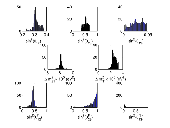
Figure 2: Frequency plots of mixing angles and mass-squared differences for $v_{R}=20$ TeV. The top and bottom rows show results for the left- and right-handed mixing angles, respectively. The middle row shows frequency plots for $\Delta m_{ij}^{2}=m_{i}^{2}-m_{j}^{2}$, the mass-squared differences for the light neutrinos. The plots in the top two rows satisfy the constraints noted in Table 1.

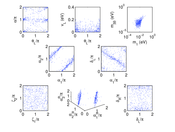
Figure 3: Plots of various phases, $v_{L}$ and $m_{\beta\beta}$ for $v_{R}=20$ TeV. The effective neutrino mass $m_{\beta\beta}$ is defined in Eq. (72).

III.2 Masses, mixings and phases for $v_{R}=20$ TeV and $v_{R}=50$ TeV

In this subsection we summarize our results for neutrino masses, mixing angles and phases for two choices for the right-handed scale, $v_{R}=20$ TeV and $v_{R}=50$ TeV. We also include some comments on $m_{\beta\beta}$, the effective neutrino mass for neutrinoless double beta decay. In the following subsection we discuss some other phenomenology of the model.

Figure 1 shows the neutrino masses obtained for the case $v_{R}=20$ TeV. The data were generated using the Monte Carlo algorithm outlined in the previous subsection. Each particular set of “input” parameters (Yukawa couplings and Higgs VEVs) yields three light neutrinos and three heavy neutrinos. The plot on the left shows the light neutrino masses and indicates that the model tends to favour non-degenerate (as opposed to quasi-degenerate) light neutrinos. The plot on the right contains the results for the heavy neutrinos. Approximate expressions for the heavy neutrino masses are given in Appendix A.1. As noted there, the two lightest right-handed neutrinos, $m_{1}^{R}$ and $m_{2}^{R}$, both have masses of order $\epsilon v_{R}$, while $m_{3}^{R}$ has a mass of order $v_{R}$. This scaling is evident in Fig. 1. Even though the right-handed scale is $20$ TeV, it is not uncommon to have $m_{1}^{R}$ below $5$ TeV. The mass splitting between $m_{1}^{R}$ and $m_{2}^{R}$ is typically of order $\epsilon^{2}v_{R}$, as is shown in Appendix A.1.

The plots in Fig. 2 show the mixing angles for the left- and right-handed MNS matrices as well as the mass-squared differences for the light neutrinos. The top two rows of plots show explicitly that the constraints on mass-squared differences and mixing angles in Table 1 are indeed satisfied by the model. The bottom row shows the right-handed mixing angles favoured by the model. Appendix A.1 contains approximate expressions for each of the right-handed mixing angles, noting that

$$\sin^{2}\theta_{12}^{R} \simeq 0.5\left(1-{\cal O}(\epsilon)\right)\;,$$

$$\sin^{2}\theta_{23}^{R} \simeq 1-{\cal O}(\epsilon^{2})\;,$$ (109)

$$\sin^{2}\theta_{13}^{R} \simeq {\cal O}(\epsilon^{4})\;.$$

The interested reader is referred to this appendix for explicit expressions in terms of the relevant Yukawa couplings. The above expressions are consistent with the results indicated in Fig. 2.

Figure 3 shows relations among the various phases appearing in the left- and right-handed MNS matrices, as well as plots of $v_{L}$ and $m_{\beta\beta}$. The upper left plot shows the correlation between $\alpha$ and $\theta_{L}$ (the phases associated with the bidoublet and left-handed triplet Higgs boson fields, respectively). It is evident from the plot that the model (or at least the numerical procedure) favours $\alpha$ near $0$ and $\pi$, although other values for $\alpha$ are not ruled out. The middle plot in the top row shows the values obtained for $v_{L}$. As expected from Eq. (87), $v_{L}$ is of order $0.1$ eV for $v_{R}=20$ TeV. The upper right plot in the figure shows that $m_{\beta\beta}$, the effective neutrino mass for neutrinoless double beta decay (see Eq. (72)), is typically of order $0.001$ or $0.002$ eV for $v_{R}=20$ TeV in this model. Such values are probably beyond the sensitivity of neutrinoless double beta decay experiments of the near future. To see why $m_{\beta\beta}$ is so small, consider its dependence on the left-handed Majorana phases $\alpha_{1}$ and $\alpha_{2}$ and the “Dirac” phase $\delta_{L}$ (shown in the middle pair of plots in Fig. 3). To a good approximation (i.e., taking $c_{13}^{2}\simeq 1$), Eq. (72) may be written as follows,

$$m_{\beta\beta}\simeq\left|m_{3}s_{13}^{2}+\left(m_{1}c_{12}^{2}-m_{2}s_{12}^{2}e^{i(\alpha_{2}-\alpha_{1}-\pi)}\right)e^{i(\alpha_{1}+2\delta_{L})}\right|\;.$$ (110)

As is evident from Fig. 3, to a good approximation, $\alpha_{2}\approx\alpha_{1}+\pi~{}(\textrm{mod}~{}2\pi)$ and there is typically a partial cancellation between the terms proportional to $m_{1}$ and $m_{2}$ in the above expression. Also, the $m_{3}$ term is suppressed by $\sin^{2}\theta_{13}$. There could in principle be interference between the terms, but the overall smallness of $m_{\beta\beta}$ would make it difficult to use $m_{\beta\beta}$ as a probe of the phases involved. The bottom row of plots in Fig. 3 shows the phases associated with the right-handed MNS matrix (see Eq. (71)). The right-handed Majorana phases $\alpha_{1}^{R}$ and $\alpha_{2}^{R}$ satisfy the approximate relation $\alpha_{2}^{R}\approx\alpha_{1}^{R}+\pi~{}(\textrm{mod}~{}2\pi)$, a result that has been derived analytically (see Appendix A.1). Scatter plots for the other right-handed phases are also shown.

A similar analysis has been performed for $v_{R}=50$ TeV and the results are qualitatively similar to those for $v_{R}=20$ TeV. The light and heavy neutrino masses obtained for that case are shown in Fig. 4. As might be expected, the heavy neutrino masses are larger than their counterparts for $v_{R}=20$ TeV and the light neutrino masses are somewhat smaller, due to the two seesaw mechanisms at work (see the discussion around Eq. (106)). Plots of the mixing angles and phases for $v_{R}=50$ TeV are similar to those in Figs. 2 and 3 and are not shown. The values obtained for $v_{L}$ and $m_{\beta\beta}$ are generally somewhat smaller for $v_{R}=50$ TeV than those that were found for $v_{R}=20$ TeV.

Figure 4: Same as in Fig. 1, but for $v_{R}=50$ TeV. Note that the axes are different here.

III.3 Some phenomenological implications

In the previous subsection we discussed neutrinoless double beta decay in the context of this model. Let us now consider some other phenomenological consequences of this model, again taking $v_{R}$ to be in the range $20$ to $50$ TeV. Incidentally, while we have not been much concerned in this work with the quark sector of the theory, we should note that many authors have studied hadronic consequences for a right-handed scale in the several-TeV range, such as effects on $B$-$\overline{B}$ and $K$-$\overline{K}$ mixing (see, for example, Refs. Beall et al. (1982); Kiers et al. (2002); Ball et al. (2000); Ball and Fleischer (2000), and references therein.) We shall not consider such effects further here, but shall be mainly concerned with leptonic phenomenology.

First let us consider the effect that a “moderate” right-handed scale has on leptogenesis. Leptogenesis provides a mechanism for generating the baryon asymmetry of the universe through CP asymmetries involving leptons Fukugita and Yanagida (1986); Luty (1992); Buchmuller and Plumacher (1996). Within the LRM, the asymmetries can occur in the decays of heavy (right-handed) neutrinos to charged leptons and Higgs bosons, as well as in the decays of left-handed Higgs triplets to pairs of charged leptons (see Refs. Hambye and Senjanovic (2004); Antusch and King (2004); Chen and Mahanthappa (2005)). The asymmetries arise through the interference of the tree-level diagrams with one-loop self-energy and vertex correction diagrams. The asymmetries for the decay of the lightest right-handed neutrino may be separated into Type I and II contributions as follows Hambye and Senjanovic (2004); Antusch and King (2004); Chen and Mahanthappa (2005) (the reason for the “Type I” designation for the first expression will be more apparent in a moment),

$$\epsilon_{\nu_{R_{1}}}^{I} = \frac{1}{4\pi(k_{1}^{2}+k_{2}^{2})}\sum_{j\neq 1}\frac{\textrm{Im}\left[\left(\widetilde{M}_{LR}^{\dagger}\widetilde{M}_{LR}\right)_{1j}^{2}\right]}{\left(\widetilde{M}_{LR}^{\dagger}\widetilde{M}_{LR}\right)_{11}}\sqrt{x_{j}}\left[1-\left(1+x_{j}\right)\ln\left(1+\frac{1}{x_{j}}\right)+\frac{1}{1-x_{j}}\right]\!,$$ (111)

$$\epsilon_{\nu_{R_{1}}}^{II} = \frac{3\,m_{1}^{R}}{4\pi(k_{1}^{2}+k_{2}^{2})}\frac{\textrm{Im}\left[\left(\widetilde{M}_{LR}^{\dagger}M_{\nu}^{II}\widetilde{M}_{LR}^{*}\right)_{11}\right]}{\left(\widetilde{M}_{LR}^{\dagger}\widetilde{M}_{LR}\right)_{11}}y\left[1-y\ln\left(1+\frac{1}{y}\right)\right]\!,$$ (112)

where $\widetilde{M}_{LR}\equiv M_{LR}V_{R}^{\nu}$ (with $V_{R}^{\nu}$ being the matrix that diagonalizes $M_{RR}$ – see Eq. (48)). Also, $x_{j}=(m_{j}^{R}/m_{1}^{R})^{2}$ and $y=(m_{\Delta_{L}}/m_{1}^{R})^{2}$, with $m_{\Delta_{L}}$ being the left-handed Higgs triplet mass (see Ref. Kiers et al. (2005)). It is instructive to consider the limits $x_{j}\gg 1$ and $y\gg 1$, in which case the asymmetries become

$$\epsilon_{\nu_{R_{1}}}^{I} \simeq \frac{3\,m_{1}^{R}}{8\pi(k_{1}^{2}+k_{2}^{2})}\frac{\textrm{Im}\left[\left(\widetilde{M}_{LR}^{\dagger}M_{\nu}^{I}\widetilde{M}_{LR}^{*}\right)_{11}\right]}{\left(\widetilde{M}_{LR}^{\dagger}\widetilde{M}_{LR}\right)_{11}}\;,$$ (113)

$$\epsilon_{\nu_{R_{1}}}^{II} \simeq \frac{3\,m_{1}^{R}}{8\pi(k_{1}^{2}+k_{2}^{2})}\frac{\textrm{Im}\left[\left(\widetilde{M}_{LR}^{\dagger}M_{\nu}^{II}\widetilde{M}_{LR}^{*}\right)_{11}\right]}{\left(\widetilde{M}_{LR}^{\dagger}\widetilde{M}_{LR}\right)_{11}}\;,$$ (114)

illustrating a nice symmetry between the two expressions Antusch and King (2004). (Recall that $M_{\nu}^{I}$ and $M_{\nu}^{II}$ are the Type I and II contributions to the light neutrino mass matrix – see Eq. (4).) We may use the above expressions to estimate the CP asymmetries within the context of this model. Assuming phases of order unity, $m_{1}^{R}\sim$10-25 TeV and $M_{\nu}^{I,II}\sim 0.05$ eV (from Figs. 1 and 4), one obtains the estimates $\left|\epsilon_{\nu_{R_{1}}}^{I}\right|,\left|\epsilon_{\nu_{R_{1}}}^{II}\right|\sim 10^{-12}$. Unfortunately, such values are far too small to account for the observed baryon asymmetry of the universe – one typically requires $\epsilon_{\nu_{R_{1}}}$ to be of order $10^{-6}$ or $10^{-7}$ Aalseth et al. (2002); Hambye and Senjanovic (2004). We have computed the asymmetries numerically for the $v_{R}=20$ and $50$ TeV data sets using the original expressions in Eqs. (111) and (112), and setting $m_{\Delta_{L}}=v_{R}$ for simplicity. We find numerically that $\left|\epsilon_{\nu_{R_{1}}}^{II}\right|\sim 10^{-13}$, with values sometimes of order $10^{-12}$. The asymmetry $\left|\epsilon_{\nu_{R_{1}}}^{I}\right|$ is typically of order $10^{-12}$ to $10^{-11}$, but is sometimes enhanced by one or more orders of magnitude. The root cause of the tiny asymmetries is the fact that the right-handed scale is so low – Eqs. (113) and (114) are both proportional to the lightest right-handed neutrino mass, which is in turn proportional to the right-handed scale. If one were to consider a much higher right-handed scale (while keeping $M_{\nu}$ fixed at its physical value of approximately $0.05$ eV), one could obtain asymmetries that are of the correct order of magnitude for leptogenesis.

While leptogenesis would require a much higher right-handed scale than we are considering in this work, a low or moderate right-handed scale has the phenomenological advantage that departures from the SM could be observable at upcoming experiments. One striking experimental signature of the LRM would be the production of like-sign leptons due to the decay of doubly-charged Higgs bosons, $\delta_{L,R}^{\pm\pm}$. Several authors have investigated the possibility of producing doubly-charged Higgs bosons at upcoming collider experiments such as the LHC Huitu et al. (1997); Maalampi and Romanenko (2002); Azuelos et al. (2005) or a linear collider Godfrey et al. (2001); Mukhopadhyaya and Rai (2005). We shall not consider direct Higgs production further here, except to note that a lower right-handed scale is obviously desirable if one hopes to produce on-shell, doubly-charged Higgs bosons. The doubly charged Higgs bosons in the LRM also generically contain lepton flavour violating (LFV) couplings, which are related to the complex symmetric matrix $F$ in Eq. (14). These couplings lead to decays such as $\mu\to 3e$ Swartz (1989), $\tau\to 3\mu$ and $\tau\to\mu ee$. Since the decays occur at tree-level in the LRM, they may be used to place indirect limits on various combinations of the LFV couplings and the doubly-charged scalar masses. We will consider some of the limits for these decays, as well as branching ratio predictions for various combinations of LFV couplings and Higgs boson masses. Other bounds on the elements of $F$ can also be obtained by considering muonium-antiuonium conversion Swartz (1989); Godfrey et al. (2001) and $\mu\to e\gamma$ Mohapatra (1992); Barenboim and Raidal (1997); Boyarkin et al. (2004).

Since the $2$-$2$ and $2$-$3$ elements of $F$ are generically rather large in our model (see Eq. (85)), let us first consider the decay $\tau^{-}\to\mu^{+}\mu^{-}\mu^{-}$. Neglecting the muon masses compared to $m_{\tau}$, we obtain the following expression for the partial width,

$$\Gamma(\tau^{-}\to\mu^{+}\mu^{-}\mu^{-})\simeq\frac{1}{2}\frac{m_{\tau}}{(32)(192\pi^{3})}\left[\left(\frac{m_{\tau}}{m_{\Delta_{L}}}\right)^{4}\left|F_{L23}F_{L22}^{*}\right|^{2}+\left(\frac{m_{\tau}}{m_{\Delta_{R}}}\right)^{4}\left|F_{R23}F_{R22}^{*}\right|^{2}\right],$$ (115)

where the factor of $1/2$ accounts for the presence of two identical particles in the final state and

$$F_{L,R}\equiv V_{L,R}^{\ell T}FV_{L,R}^{\ell}\;.$$ (116)

The matrices $V_{L,R}^{\ell}$ in the above expression are those that were used to diagonalize the charged lepton mass matrix in Eq. (26). $V_{L}^{\ell}$ and $V_{R}^{\ell}$ both typically involve small mixing angles (see the discussion in Appendix A.1). A cross-term involving $F_{L}$ and $F_{R}$ has been dropped from Eq. (115) because its leading behaviour is proportional to $m_{\mu}^{3}$. The masses of the doubly-charged Higgs bosons were calculated approximately in Ref. Kiers et al. (2005) for this model. For our purposes it is sufficient to keep the leading terms,

$$m_{\Delta_{L}}^{2} \simeq \left(\frac{1}{2}\widetilde{\rho}_{3}-\widetilde{\rho}_{1}\right)v_{R}^{2}\;,$$ (117)

$$m_{\Delta_{R}}^{2} \simeq 2\widetilde{\rho}_{2}v_{R}^{2}\;,$$ (118)

where the constants $\widetilde{\rho}_{1}$, $\widetilde{\rho}_{2}$ and $\widetilde{\rho}_{3}$ are dimensionless coefficients in the Higgs potential that are generically of order unity in the horizontal symmetry model.

Table 2: Doubly-charged Higgs masses and corresponding branching ratios for various LFV decays. As described in the text, we assume that $m_{\Delta_{L}}=m_{\Delta_{R}}\equiv m_{\Delta}$, that $F_{L}$ and $F_{R}$ scale in approximately the same way as $F$ (see Eq. (85)) and that the “order unity coefficients” in these matrices each take on the value “3.” The entries in the third column give Higgs boson masses that would yield branching ratios at the current experimental limits. The branching ratios for the rare $\tau$ decays are taken from Ref. Yusa et al. (2004) and that for $\mu^{-}\to e^{+}e^{-}e^{-}$ is taken from Ref. Eidelman et al. (2004). The sixth column gives the branching ratios that would be obtained for the Higgs boson masses indicated in the fifth column.

process	matrix elements	$m_{\Delta}$	exp’l BR ($90\%$ c.l.)	$m_{\Delta}$	future BR
$\tau^{-}\to\mu^{+}\mu^{-}\mu^{-}$	$\left|F_{23}F_{22}^{*}\right|=(3\epsilon)\times(3)$	6.2 TeV	$2.0\times 10^{-7}$	20 TeV	$2.0\times 10^{-9}$
$\tau^{-}\to\mu^{+}e^{-}\mu^{-}$	$\left|F_{23}F_{12}^{*}\right|=(3\epsilon)\times(3\epsilon^{2})$	2.2 TeV	$2.0\times 10^{-7}$	7.0 TeV	$2.0\times 10^{-9}$
$\tau^{-}\to e^{+}\mu^{-}\mu^{-}$	$\left|F_{13}F_{22}^{*}\right|=(3\epsilon)\times(3)$	6.2 TeV	$2.0\times 10^{-7}$	20 TeV	$2.0\times 10^{-9}$
$\tau^{-}\to e^{+}e^{-}\mu^{-}$	$\left|F_{13}F_{12}^{*}\right|=(3\epsilon)\times(3\epsilon^{2})$	2.2 TeV	$1.9\times 10^{-7}$	7.0 TeV	$2.0\times 10^{-9}$
$\mu^{-}\to e^{+}e^{-}e^{-}$	$\left|F_{12}F_{11}^{*}\right|=(3\epsilon^{2})\times(3\epsilon^{4})$	10 TeV	$1.0\times 10^{-12}$	18 TeV	$1.0\times 10^{-13}$

The first row of Table 2 gives a few numerical estimates for the decay $\tau^{-}\to\mu^{+}\mu^{-}\mu^{-}$ assuming, for the sake of simplicity, that $m_{\Delta_{L}}=m_{\Delta_{R}}\equiv m_{\Delta}$ We also assume that $F_{L}$ and $F_{R}$ both scale in the same way as $F$ (see Eq. (85)) and that the “order unity” coefficients in the elements of $F_{L}$ and $F_{R}$ all have a magnitude of “3.” Under these assumptions, the left- and right-handed contributions to Eq. (115) are equal. Results are also included for several other LFV decay modes. The expressions for those decays are similar to Eq. (115), with appropriate changes in the matrix elements of $F_{L}$ and $F_{R}$ and the deletion of the factor of “$1/2$” in cases in which the final state does not contain identical particles. The entries in the fourth column of the table give upper limits on the experimental branching ratios at the $90\%$ c.l. The third column lists the Higgs boson masses that would yield branching ratios right at the experimental limits. The decay $\mu\to 3e$ currently gives the furthest reach in terms of the doubly-charged Higgs boson mass, even though $F_{11}$ is generically the smallest element of $F$ in this model. The fifth and sixth columns list some representative values for slightly larger Higgs boson masses and what the corresponding branching ratios would be. For the rare $\mu$ decay we have assumed an order of magnitude improvement in the sensitivity. For the rare $\tau$ decays we have assumed a branching ratio of $2\times 10^{-9}$, consistent with the “several times $10^{-9}$” sensitivity possible at a Super B factory Akeroyd et al. (2004). A Super B Factory could probe doubly-charged Higgs boson masses at the 20 TeV level.

IV Discussion and Conclusions

In this work we have studied the lepton sector of a Left-Right Model with a low right-handed symmetry breaking scale. Such a model can be made phenomenologically viable if the underlying $SU(2)_{L}\times SU(2)_{R}\times U(1)$ gauge symmetry of the theory is supplemented by a $U(1)$ horizontal symmetry to suppress relevant Yukawa couplings. We have analyzed the parameter space of this model numerically with the help of a Monte-Carlo approach. The model is able to reproduce the main features of the lepton mass spectrum and is able to accomodate experimental constraints on the mixing angles and mass-squared differences of light neutrinos.

We have also discussed other phenomenological applications of this model, such as lepton-flavor-violating transitions, which occur due to the presence of doubly-charged Higgs bosons in the theory. These transitions produce the most striking experimental signatures of the model. We have considered LFV decays of the type $\tau^{\pm}\to\mu^{\mp}\mu^{\pm}\mu^{\pm}$, which constrain both the masses and couplings of these Higgs bosons. While the currently-available experimental bounds on such decays probe the mass ranges of a few TeV for the doubly charged Higgs bosons, a two-order of magnitude improvement in the experimental bound for the branching ratios of $\tau^{\pm}\to\mu^{\mp}\mu^{\pm}\mu^{\pm}$ and $\tau^{\pm}\to e^{\mp}\mu^{\pm}\mu^{\pm}$ would probe the relevant mass scale of tens of TeV. We have noted that a LRM with such a low right-handed symmetry breaking scale does not accomodate the required CP-violating asymmetries needed for generating the baryon asymmetry of the universe via leptogenesis. Leptogenesis would generally require a much higher right-handed scale. We have also calculated the effective mass for neutrinoless double beta decay for this model. The resulting values are probably beyond the sensitivity of experiments of the near future.

*

Appendix A Derivation of some approximate results

In the first part of the Appendix we derive some approximate results for right-handed neutrinos. Following that we comment on the possibility of obtaining large mixing angles in this model.

A.1 Approximate relations for right-handed neutrinos

As is clear from Fig. 2, the mixing angles for the right-handed MNS matrix are such that $\sin^{2}\theta_{12}^{R}\sim 0.5$, $\sin^{2}\theta_{23}^{R}\sim 1$ and $\sin^{2}\theta_{13}^{R}\sim 0$. In this subsection of the Appendix we outline an approximate calculation of the three mixing angles, showing that, indeed,

$$\sin^{2}\theta_{12}^{R} \simeq 0.5\left(1-{\cal O}(\epsilon)\right)\;,$$

$$\sin^{2}\theta_{23}^{R} \simeq 1-{\cal O}(\epsilon^{2})\;,$$ (119)

$$\sin^{2}\theta_{13}^{R} \simeq {\cal O}(\epsilon^{4})\;.$$

More precise expressions for the right-handed mixing angles may be found below. We also determine approximate analytical expressions for the heavy neutrino masses.

To determine the right-handed MNS matrix, one must first diagonalize the charged lepton mass matrix, $M_{\ell}$, and the mass matrix for heavy (right-handed) neutrinos, $M_{RR}$. Diagonalization of these two matrices yields the unitary matrices $V_{L}^{\ell}$, $V_{R}^{\ell}$ and $V_{R}^{\nu}$ (see Eqs. (26) and (48)). The latter two of these are used to form the right-handed MNS matrix, as seen in Eq. (50),

$$\widetilde{\cal U}_{R}^{MNS} = V_{R}^{\ell\dagger}V_{R}^{\nu}\;.$$

The “tilde” indicates that the MNS matrix still needs to be rephased to bring it into the usual form – see Eqs. (51) and (52). Our approximate calculation makes use of the fact that we have two small quantities with which to perform an expansion. The first, $\epsilon$, is the parameter that breaks the horizontal symmetry in our model. Although this parameter is not particularly small (we take $\epsilon=0.3$ throughout this paper), it still does allow for some progress. The second small parameter in our calculation is the ratio of the bidoublet Higgs VEVs, assumed to be $k_{2}/k_{1}=3/181\sim\epsilon^{4}$.

Consider first the charged lepton mass matrix, given in Eq. (25). Taking into account the small value for the ratio $k_{2}/k_{1}$ and the scaling of the Yukawa matrices in (85), it is clear that $M_{\ell}$ is dominated by the term proportional to $k_{1}$; i.e.,

$$M_{\ell}\simeq\frac{1}{\sqrt{2}}Hk_{1}\;.$$ (120)

(The term proportional to $k_{2}$ is suppressed by an overall factor of approximately $\epsilon^{8}$.) Since $H$ is Hermitian and $k_{1}$ is real, $M_{\ell}$ is also Hermitian in this approximation. Thus, to a good approximation, $M_{\ell}$ may be diagonalized by a single unitary matrix (c.f. the general biunitary transformation shown in Eq. (26)). To the extent that $M_{\ell}$ is Hermitian, the resulting diagonalized mass matrix has real eigenvalues, although some of them would possibly be negative. A diagonal sign matrix ($\pm 1$ along the diagonal) can then be used to correct the signs on the masses. Thus, to a good approximation, $V_{R}^{\ell}$ and $V_{L}^{\ell}$ in Eq. (26) are related,

$$V_{L}^{\ell}\simeq V_{R}^{\ell}A_{\ell}^{\textrm{\scriptsize{sign}}}\;,$$ (121)

where $A_{\ell}^{\textrm{\scriptsize{sign}}}$ is a sign matrix used to make the charged lepton masses positive, and we have

$$M_{\ell}^{\textrm{\scriptsize diag}}\simeq A_{\ell}^{\textrm{\scriptsize{sign}}}V_{R}^{\ell\dagger}\left(\frac{1}{\sqrt{2}}Hk_{1}\right)V_{R}^{\ell}\;.$$ (122)

It is convenient to parameterize $V_{R}^{\ell}$ as a product of three $2\times 2$ unitary rotations, as in Eq. (70). For our purposes we define

$$V_{R}^{\ell}={\cal A}_{\ell}\;{\cal U}^{(0)}(\theta_{12}^{\ell},\theta_{23}^{\ell},\theta_{13}^{\ell},\delta^{\ell})\;,$$ (123)

where ${\cal A}_{\ell}$ is a diagonal phase matrix. The diagonalization proceeds in the following order: (a) diagonal phase rotation, (b) orthogonal $2$-$3$ rotation, (c) unitary $1$-$3$ rotation (including the phase $\delta^{\ell}$), (d) orthogonal $1$-$2$ rotation. The form of the matrix $H$,

$$H\sim\left(\begin{array}[]{ccc}\epsilon^{10}&\epsilon^{8}&\epsilon^{7}\\ \epsilon^{8}&\epsilon^{6}&\epsilon^{5}\\ \epsilon^{7}&\epsilon^{5}&\epsilon^{4}\\ \end{array}\right)\;,$$ (127)

allows us to treat all of the $\theta_{ij}^{\ell}$ in Eq. (123) as small quantities. The approximate diagonalization yields $\theta_{12}^{\ell}\sim{\cal O}(\epsilon^{2})$, $\theta_{23}^{\ell}\sim{\cal O}(\epsilon)$ and $\theta_{13}^{\ell}\sim{\cal O}(\epsilon^{3})$ (we do not give the analytical expressions here).

A similar procedure may be followed to diagonalize the matrix $M_{RR}=Fv_{R}/\sqrt{2}$. Since $M_{RR}$ is complex-symmetrix (not Hermitian), the diagonalization is performed using a unitary matrix and its transpose (rather than a unitary matrix and its Hermitian conjugate),

$$M_{R}^{\textrm{\scriptsize diag}} = V_{R}^{\nu T}\left(\frac{1}{\sqrt{2}}Fv_{R}\right)V_{R}^{\nu}\;.$$ (128)

We parameterize $V_{R}^{\nu}$ as

$$V_{R}^{\nu}={\cal A}_{\nu}\;{\cal U}^{(0)}(\theta_{12}^{\nu},\theta_{23}^{\nu},\theta_{13}^{\nu},\delta^{\nu}){\cal B}_{\nu}\;,$$ (129)

where ${\cal A}_{\nu}$ and ${\cal B}_{\nu}$ are both diagonal phase matrices. The form of the complex-symmetric Yukawa matrix $F$,

$$F\sim\left(\begin{array}[]{ccc}\epsilon^{4}&\epsilon^{2}&\epsilon\\ \epsilon^{2}&1&\epsilon\\ \epsilon&\epsilon&\epsilon^{2}\\ \end{array}\right),$$ (133)

yields some clues as to how to proceed with the diagonalization. First of all, we wish to order the eigenvalues in ascending order (by magnitude), so the $2$-$2$ element needs to be moved to the $3$-$3$ location. This is accomplished using the $2$-$3$ rotation that occurs immediately following the initial phase rotation. Since $\theta_{23}^{\nu}$ is evidently close to $\pi/2$, we take $\cos\theta_{23}^{\nu}$ to be a small quantity for the purpose of our approximate calculation. $\theta_{13}^{\nu}$ is similarly regarded as a small quantity. Performing these first three rotations (the diagonal phase rotation associated with ${\cal A}_{\nu}$, the $2$-$3$ rotation and the $1$-$3$ rotation) yields the following partly diagonalized mass matrix,

$$\left.M_{RR}\right|_{23,13}\simeq\frac{v_{r}}{\sqrt{2}}\left(\begin{array}[]{ccc}{\cal O}(\epsilon^{4})&{\cal O}(\epsilon)&0\\ {\cal O}(\epsilon)&{\cal O}(\epsilon^{2})&0\\ 0&0&{\cal O}(1)\\ \end{array}\right)\;.$$ (137)

Clearly the remaining $1$-$2$ rotation must be “large.” Neglecting the $1$-$1$ element in the above expression, it is straightforward to determine an approximate expression for $\sin\theta_{12}^{\nu}$ in terms of the $1$-$2$ and $2$-$2$ elements and to verify that $\theta_{12}^{\nu}\sim\pi/4$.

Combining the approximate expressions obtained for $V_{R}^{\ell}$ and $V_{R}^{\nu}$, we may finally determine an approximate expression for the right-handed MNS matrix. Expanding the expression in terms of $\epsilon$, we obtain the following approximate relation for $\sin\theta_{12}^{R}$,

$$\sin\theta_{12}^{R}\simeq\sin\theta_{12}^{\nu}\simeq\frac{\sqrt{2}|a|}{\left[\sqrt{4|a|^{2}+|b|^{2}}\left(|b|+\sqrt{4|a|^{2}+|b|^{2}}\right)\right]^{1/2}}\;,$$ (138)

where

$$a=F_{13}={\cal O}(\epsilon)$$ (139)

and

$$b=F_{33}-\frac{F_{23}^{2}}{F_{22}}={\cal O}(\epsilon^{2})\;.$$ (140)

Then,

$$\sin\theta_{12}^{R}=\frac{1}{\sqrt{2}}\left(1-{\cal O}(\epsilon)\right)\;.$$ (141)

For the other two mixing angles we obtain

$$\cos\theta_{23}^{R} \simeq \left|\frac{F_{23}}{F_{22}}+\frac{H_{23}}{H_{33}}\right|={\cal O}(\epsilon)\;,$$ (142)

$$\sin\theta_{13}^{R} \simeq \left|\frac{F_{12}^{*}}{F_{22}}+\frac{F_{13}^{*}F_{23}}{F_{22}^{2}}-\frac{\left(H_{12}H_{33}-H_{13}H_{23}^{*}\right)}{\left(H_{22}H_{33}-\left|H_{23}\right|^{2}\right)}\right|={\cal O}(\epsilon^{2})\;.$$ (143)

(Recall that $F_{22}$, $H_{12}$, $H_{13}$, $H_{33}$ and $H_{22}$ are all taken to be real in this work, as discussed in Sec. II.2.) Note that the $2$-$3$ and $1$-$3$ mixing angles receive comparable contributions from the diagonalizations of $M_{\ell}$ and $M_{RR}$, while the $1$-$2$ mixing angle is determined almost exclusively by the diagonalization of $M_{RR}$. The above approximate expressions for the three right-handed mixing angles agree relatively well with the results obtained by performing the diagonalizations numerically, except for cases in which the approximations break down (such as when a denominator in one of the expressions involved is accidentally close to zero).

Having performed an approximate diagonalization of $M_{RR}$ to obtain the mixing angles, it is also straightforward to obtain approximate expressions for the three heavy neutrino masses. We find

$$m_{1}^{R} \simeq \frac{v_{R}}{2\sqrt{2}}\left[\sqrt{4|a|^{2}+|b|^{2}}-|b|\right]={\cal O}(\epsilon v_{R})\;,$$ (144)

$$m_{2}^{R} \simeq \frac{v_{R}}{2\sqrt{2}}\left[\sqrt{4|a|^{2}+|b|^{2}}+|b|\right]={\cal O}(\epsilon v_{R})\;,$$ (145)

$$m_{3}^{R} \simeq \frac{v_{R}}{\sqrt{2}}F_{22}={\cal O}(v_{R})\;,$$ (146)

which leads to the following approximate relation between $m_{1}^{R}$ and $m_{2}^{R}$ in this model,

$$m_{2}^{R}-m_{1}^{R}\simeq\frac{v_{r}}{\sqrt{2}}\left|F_{33}-\frac{F_{23}^{2}}{F_{22}}\right|={\cal O}(\epsilon^{2}v_{r})\;.$$ (147)

We may also determine the largest value we might expect for $m_{1}^{R}$ in our numerical work (given that “order unity” coefficients are required to have a magnitude between zero and 3). Setting $b=0$ and $|a|=3\epsilon$ we obtain

$$m_{1,\textrm{\scriptsize{max}}}^{R}\simeq\frac{3\epsilon v_{R}}{\sqrt{2}}\;.$$ (148)

For $v_{R}=20$ TeV, $m_{1,\textrm{\scriptsize{max}}}^{R}\simeq 13$ TeV and for $v_{R}=50$ TeV, $m_{1,\textrm{\scriptsize{max}}}^{R}\simeq 32$ TeV, consistent with Figs. 1 and 4, respectively. The largest values for $m_{3}^{R}$ typically occur when $F_{22}\sim 3$, yielding $m_{3,\textrm{\scriptsize{max}}}^{R}\simeq 42$ TeV for $v_{R}=20$ TeV and $m_{3,\textrm{\scriptsize{max}}}^{R}\simeq 110$ TeV for $v_{R}=50$ TeV. The approximate expressions for the masses of the three heavy neutrinos agree relatively well with the values obtained numerically (except for cases in which the approximations break down, as described above).

The approximate diagonalization procedure also allows us to derive an approximate relation between $\alpha_{1}^{R}$ and $\alpha_{2}^{R}$, two of the right-handed Majorana phases. To a good approximation we obtain $\alpha_{2}^{R}\simeq\alpha_{1}^{R}+\pi$ (mod $2\pi$), a relation that is evident in Fig. 3.

A.2 A few comments on obtaining large mixing angles

The authors of Ref. Khasanov and Perez (2002) noted that it would be difficult or impossible to obtain large $1$-$2$ mixing in this model. Looking at Eq. (106), it would appear that the $1$-$2$ and $2$-$3$ angles should indeed be small generically. Yet our Monte Carlo algorithm does find order-unity sets of coefficients for $\widetilde{F}$, $\widetilde{G}$ and $\widetilde{H}$ that yield neutrino masses and mixings consistent with experiment (i.e., with large $1$-$2$ and $2$-$3$ mixing angles). To understand how this can happen, note that the diagonalization of the neutrino mass matrix may be understood to proceed in several steps, beginning with a $2$-$3$ rotation, which is followed by a $1$-$3$ rotation and finally by a $1$-$2$ rotation. Experimentally, the $2$-$3$ rotation is large (of order $\pi/4$), the $1$-$3$ rotation is small and the $1$-$2$ rotation is large (of order $\pi/6$ or $\pi/5)$. To simplify our discussion, let us consider a case study of a neutrino mass matrix that was obtained for the case $v_{R}=20$ TeV. The magnitudes of the elements of the mass matrix had the following values after each stage of the diagonalization:

$$M_{\nu}\sim\left(\begin{array}[]{ccc}0.0015&0.0061&0.014\\ 0.0061&0.033&0.025\\ 0.014&0.025&0.020\\ \end{array}\right)~{}\mbox{eV} \stackrel{{\scriptstyle\textrm{\scriptsize{2-3}}}}{{\longrightarrow}} \left(\begin{array}[]{ccc}0.0015&0.010&0.011\\ 0.010&0.0070&0.0021\\ 0.011&0.0021&0.052\\ \end{array}\right)~{}\mbox{eV}$$ (155)

$$\stackrel{{\scriptstyle\textrm{\scriptsize{1-3}}}}{{\longrightarrow}} \left(\begin{array}[]{ccc}0.0038&0.011&0\\ 0.011&0.0070&0\\ 0&0&0.054\\ \end{array}\right)~{}\mbox{eV}$$ (159)

$$\stackrel{{\scriptstyle\textrm{\scriptsize{1-2}}}}{{\longrightarrow}} \left(\begin{array}[]{ccc}0.010&0&0\\ 0&0.014&0\\ 0&0&0.054\\ \end{array}\right)~{}\mbox{eV}\;.$$ (163)

The mixing angles for the diagonalization of this mass matrix were “typical;” i.e., the $2$-$3$ rotation angle was approximately $\pi/(3.6)$, the $1$-$3$ rotation was small and the $1$-$2$ rotation was approximately $\pi/(5.6)$. The first thing that is clear is that the original mass matrix does not have the hierarchy described in Eq. (106). In particular, the $2$-$3$ block is approximately degenerate and is suppressed relative to the “generic” expression. That the $2$-$3$ block is quasi-degenerate is perhaps not a surprise, given that the $2$-$3$ rotation angle needs to be close to $\pi/4$. The elements of the $1$-$2$ block of the original mass matrix have approximately the expected magnitudes, with the ratio $\left|M_{\nu 12}/M_{\nu 22}\right|$ being relatively small. Following the (large) $2$-$3$ rotation and the (small) $1$-$3$ rotation, the $1$-$2$ block is in a form suitable for a relatively large $1$-$2$ rotation. The neutrino mass matrix in this case study is fairly typical in that the neutrino mass matrices that yield experimentally viable mixing angles tend to have suppressed (and quasi-degenerate) $2$-$3$ blocks compared to the “generic” expectation in Eq. (106). Some of the suppression is due to a suppression of $F^{-1}$ compared to the expression in Eq. (91).

References

- Pati and Salam (1974) J. C. Pati and A. Salam, Phys. Rev. D10, 275 (1974).
- Mohapatra and Pati (1975a) R. N. Mohapatra and J. C. Pati, Phys. Rev. D11, 566 (1975a).
- Mohapatra and Pati (1975b) R. N. Mohapatra and J. C. Pati, Phys. Rev. D11, 2558 (1975b).
- Senjanovic and Mohapatra (1975) G. Senjanovic and R. N. Mohapatra, Phys. Rev. D12, 1502 (1975).
- Mohapatra et al. (1978) R. N. Mohapatra, F. E. Paige, and D. P. Sidhu, Phys. Rev. D17, 2462 (1978).
- Senjanovic (1979) G. Senjanovic, Nucl. Phys. B153, 334 (1979).
- Duka et al. (2000) P. Duka, J. Gluza, and M. Zralek, Annals Phys. 280, 336 (2000), eprint hep-ph/9910279.
- Ball et al. (2000) P. Ball, J. M. Frere, and J. Matias, Nucl. Phys. B572, 3 (2000), eprint hep-ph/9910211.
- Kiers et al. (2002) K. Kiers, J. Kolb, J. Lee, A. Soni, and G.-H. Wu, Phys. Rev. D66, 095002 (2002), eprint hep-ph/0205082.
- Kiers et al. (2005) K. Kiers, M. Assis, and A. A. Petrov, Phys. Rev. D71, 115015 (2005), eprint hep-ph/0503115.
- Fukugita and Yanagida (1986) M. Fukugita and T. Yanagida, Phys. Lett. B174, 45 (1986).
- Luty (1992) M. A. Luty, Phys. Rev. D45, 455 (1992).
- Buchmuller and Plumacher (1996) W. Buchmuller and M. Plumacher, Phys. Lett. B389, 73 (1996), eprint hep-ph/9608308.
- Hambye and Senjanovic (2004) T. Hambye and G. Senjanovic, Phys. Lett. B582, 73 (2004), eprint hep-ph/0307237.
- Antusch and King (2004) S. Antusch and S. F. King, Phys. Lett. B597, 199 (2004), eprint hep-ph/0405093.
- Chen and Mahanthappa (2005) M.-C. Chen and K. T. Mahanthappa, Phys. Rev. D71, 035001 (2005), eprint hep-ph/0411158.
- Atwood et al. (2005) D. Atwood, S. Bar-Shalom, and A. Soni (2005), eprint hep-ph/0502234.
- Mohapatra and Senjanovic (1981) R. N. Mohapatra and G. Senjanovic, Phys. Rev. D23, 165 (1981).
- Deshpande et al. (1991) N. G. Deshpande, J. F. Gunion, B. Kayser, and F. Olness, Phys. Rev. D44, 837 (1991).
- Mohapatra (2001) R. N. Mohapatra, Nucl. Phys. Proc. Suppl. 91, 313 (2001), eprint hep-ph/0008232.
- Chang et al. (1984) D. Chang, R. N. Mohapatra, and M. K. Parida, Phys. Rev. Lett. 52, 1072 (1984).
- Chang and Mohapatra (1985) D. Chang and R. N. Mohapatra, Phys. Rev. D32, 1248 (1985).
- Froggatt and Nielsen (1979) C. D. Froggatt and H. B. Nielsen, Nucl. Phys. B147, 277 (1979).
- Leurer et al. (1993) M. Leurer, Y. Nir, and N. Seiberg, Nucl. Phys. B398, 319 (1993), eprint hep-ph/9212278.
- Khasanov and Perez (2002) O. Khasanov and G. Perez, Phys. Rev. D65, 053007 (2002), eprint hep-ph/0108176.
- Kayser (2002) B. Kayser (2002), eprint hep-ph/0211134.
- Langacker and Uma Sankar (1989) P. Langacker and S. Uma Sankar, Phys. Rev. D40, 1569 (1989).
- Bilenky et al. (2003) S. M. Bilenky, C. Giunti, J. A. Grifols, and E. Masso, Phys. Rept. 379, 69 (2003), eprint hep-ph/0211462.
- (29) Neutrinoless Double Beta Decay, http://www.nu.to.infn.it/Neutrinoless_Double_Beta_Decay/.
- Klapdor-Kleingrothaus et al. (2001) H. V. Klapdor-Kleingrothaus, A. Dietz, H. L. Harney, and I. V. Krivosheina, Mod. Phys. Lett. A16, 2409 (2001), eprint hep-ph/0201231.
- Klapdor-Kleingrothaus et al. (2004) H. V. Klapdor-Kleingrothaus, A. Dietz, I. V. Krivosheina, and O. Chkvorets, Nucl. Instrum. Meth. A522, 371 (2004), eprint hep-ph/0403018.
- Feruglio et al. (2002) F. Feruglio, A. Strumia, and F. Vissani, Nucl. Phys. B637, 345 (2002), eprint hep-ph/0201291.
- Aalseth et al. (2002) C. E. Aalseth et al., Mod. Phys. Lett. A17, 1475 (2002), eprint hep-ex/0202018.
- Choubey and Rodejohann (2005) S. Choubey and W. Rodejohann (2005), eprint hep-ph/0506102.
- Barenboim et al. (2002) G. Barenboim, M. Gorbahn, U. Nierste, and M. Raidal, Phys. Rev. D65, 095003 (2002), eprint hep-ph/0107121.
- Eidelman et al. (2004) S. Eidelman et al. (Particle Data Group), Phys. Lett. B592, 1 (2004).
- Maltoni et al. (2004) M. Maltoni, T. Schwetz, M. A. Tortola, and J. W. F. Valle, New J. Phys. 6, 122 (2004), eprint hep-ph/0405172.
- Beall et al. (1982) G. Beall, M. Bander, and A. Soni, Phys. Rev. Lett. 48, 848 (1982).
- Ball and Fleischer (2000) P. Ball and R. Fleischer, Phys. Lett. B475, 111 (2000), eprint hep-ph/9912319.
- Huitu et al. (1997) K. Huitu, J. Maalampi, A. Pietila, and M. Raidal, Nucl. Phys. B487, 27 (1997), eprint hep-ph/9606311.
- Maalampi and Romanenko (2002) J. Maalampi and N. Romanenko, Phys. Lett. B532, 202 (2002), eprint hep-ph/0201196.
- Azuelos et al. (2005) G. Azuelos, K. Benslama, and J. Ferland (2005), eprint hep-ph/0503096.
- Godfrey et al. (2001) S. Godfrey, P. Kalyniak, and N. Romaneneko (2001), eprint hep-ph/0111191.
- Mukhopadhyaya and Rai (2005) B. Mukhopadhyaya and S. K. Rai (2005), eprint hep-ph/0508290.
- Swartz (1989) M. L. Swartz, Phys. Rev. D40, 1521 (1989).
- Mohapatra (1992) R. N. Mohapatra, Phys. Rev. D46, 2990 (1992).
- Barenboim and Raidal (1997) G. Barenboim and M. Raidal, Nucl. Phys. B484, 63 (1997), eprint hep-ph/9607281.
- Boyarkin et al. (2004) O. M. Boyarkin, G. G. Boyarkina, and T. I. Bakanova, Phys. Rev. D70, 113010 (2004).
- Yusa et al. (2004) Y. Yusa et al. (Belle), Phys. Lett. B589, 103 (2004), eprint hep-ex/0403039.
- Akeroyd et al. (2004) A. G. Akeroyd et al. (SuperKEKB Physics Working Group) (2004), eprint hep-ex/0406071.