KINATION-DOMINATED REHEATING AND
COLD DARK MATTER ABUNDANCE

Abstract

      We consider the decay of a massive particle under the complete or partial domination of the kinetic energy density generated by a quintessential exponential model and we impose a number of observational constraints, originating from nucleosynthesis, the present acceleration of the universe and the dark-energy-density parameter. We show that the presence of kination causes a prolonged period during which the temperature is frozen to a plateau value, much lower than the maximal temperature achieved during the process of reheating in the absence of kination. The decoupling of a cold dark matter particle during this period is analyzed, its relic density is calculated both numerically and semi-analytically and the results are compared with each other. Using plausible values (from the viewpoint of particle models) for the mass and the thermal averaged cross section times the velocity of the cold relic, we investigate scenaria of equilibrium or non-equilibrium production. In both cases, acceptable results for the cold dark matter abundance can be obtained, by constraining the initial energy density of the decaying particle, its decay width, its mass and the averaged number of the produced cold relics. The required plateau value of the temperature is, in most cases, lower than about $40~{}{\rm GeV}$.

Keywords: Cosmology, Dark Matter, Dark Energy
PACS codes: 98.80.Cq, 95.35.+d, 98.80.-k

Published in Nucl. Phys. B751, 129 (2006)

1 INTRODUCTION

A plethora of recent data [1, 2] indicates that the energy-density content of the universe is comprised of Cold (mainly [3]) Dark Matter (CDM) and Dark Energy (DE) with density parameters [1]:

$${\sf(a)}~{}~{}\Omega_{\rm CDM}=0.24\pm 0.1~{}~{}\mbox{and}~{}~{}{\sf(b)}~{}~{}\Omega_{\rm DE}=0.73\pm 0.12,$$ (1)

respectively, at $95\%$ confidence level (c.l.). Several candidates and scenarios have been proposed so far for the explanation of these two unknown substances.

As regards CDM, the most natural candidates [4] are the weekly interacting massive particles, $\chi$’s. The most popular of these is the lightest supersymmetric (SUSY) particle (LSP) [5]. However, other candidates [6] arisen in the context of the extra dimensional theories should not be disregarded. In light of eq. (1), the $\chi$-relic density, $\Omega_{\chi}h^{2}$, is to satisfy the following range of values:

$${\sf(a)}~{}~{}0.09\lesssim\Omega_{\chi}h^{2}~{}~{}\mbox{and}~{}~{}{\sf(b)}~{}~{}\Omega_{\chi}h^{2}\lesssim 0.13.$$ (2)

Obviously, the $\Omega_{\chi}h^{2}$ calculation crucially depends on the adopted assumptions. According to the standard cosmological scenario (SC) [7], $\chi$’s (i) are produced through thermal scatterings in the plasma, (ii) reach chemical equilibrium with plasma and (iii) decouple from the cosmic fluid at a temperature $T_{\rm F}\sim(10-20)~{}{\rm GeV}$ during the radiation-dominated (RD) era (we do not consider in our analysis, modification to the Friedmann equations due to a low brane-tension as in ref. [8] and some other CDM candidates (see e.g. ref. [9]) which require a somehow different cosmological set-up). The assumptions above fix the form of the relevant Boltzmann equation, the required strength of the $\chi$ interactions for equilibrium production (EP) and lead to an isentropic cosmological evolution during the $\chi$ decoupling: The Hubble parameter is $H\propto T^{2}$ with temperature $T\propto R^{-1}$ ($R$: the scale factor of the universe). In this context, the $\Omega_{\chi}h^{2}$ calculation depends only on two parameters: The $\chi$ mass, $m_{\chi}$ and the thermal-averaged cross section of $\chi$ times velocity, $\langle\sigma v\rangle$. If, in addition, a specific particle model is adopted, $\langle\sigma v\rangle$ can be derived from $m_{\chi}$ and the residual particle spectrum of the theory (see e.g. refs. [6, 11]). Consequently, by imposing the CDM constraint – eq. (2) – some particle models (such as the Constrained Minimal SUSY Model (CMSSM) [10, 11]) can be severely restricted whereas some others (e.g. the models of refs. [12] and [13] which produce higgsino or wino LSP respectively) can be characterized as cosmologically uninteresting due to the very low obtained $\Omega_{\chi}h^{2}$.

In a couple of recent papers [14, 15], we investigated model-independently (from the viewpoint of particle physics) how the calculation of $\Omega_{\chi}h^{2}$ is modified, when one or more of the assumptions of the SC are lifted (for similar explorations, see refs. [16, 17, 18, 19, 20]). Namely, in ref. [14] we assumed that $\chi$’s (i^′) decouple during a decaying-massive-particle, $\phi$, dominated era (and mainly before reheating) (ii^′) do or do not reach chemical equilibrium with the thermal bath (iii^′) are produced by thermal scatterings and directly by the $\phi$ decay (which, naturally arises even without direct coupling [21]). The key point in our investigation is that the reheating process is not instantaneous [22]. During its realization, the maximal temperature, $T_{\rm max}$, is much larger than the so-called reheat temperature, $T_{\rm RH}$, which can be taken to be lower than $T_{\rm F}$. Also, for $T>T_{\rm RH}$, $H\propto T^{4}$ with $T\propto R^{-3/8}$ and an entropy production occurs (in contrast with the SC). As a consequence, in the context of this (let name it, Low Reheating) scenario (LRS) the $\Omega_{\chi}h^{2}$ calculation depends also on $T_{\rm RH}$, the mass of the decaying particle, $m_{\phi}$, and the averaged number of the produced $\chi$’s, $N_{\chi}$. We found [14] that, for fixed $m_{\chi}$ and $\langle\sigma v\rangle$, comfortable satisfaction of eq. (2) can be achieved by constraining $T_{\rm RH}$ (to values lower than $20~{}{\rm GeV}$), $m_{\phi}$ and $N_{\chi}$. E.g., $\Omega_{\chi}h^{2}$ decreases with respect to (w.r.t) its value in the SC [23] for low $N_{\chi}$’s and increases for larger $N_{\chi}$’s [24, 25] (with fixed $m_{\chi}$ and $\langle\sigma v\rangle$). Both EP and non-EP are possible for commonly obtainable $\langle\sigma v\rangle$’s [26].

Another role that a scalar field could play when it does not couple to matter (in contrast with the former case) is this of quintessence [29]. This scalar field $q$ (not to be confused with the deceleration parameter [3]) is supposed to roll down its potential undergoing three phases during its cosmological evolution: Initially its kinetic energy, which decreases as $T^{6}$, dominates and gives rise to a possible novel period in the universal history termed “kination” [30]. Then, $q$ freezes to a value close to the Planck scale and by now its potential energy, adjusted so that eq. (1b) is met, becomes dominant. In ref. [15], we focused on a range of the exponential potential [31] parameters, which can lead to a simultaneous satisfaction of several observational data (arising from nucleosynthesis, acceleration of the universe and the DE density parameter) in conjunction with the existence of an early totally kination-dominated (KD) era, for a reasonable region of initial conditions [32, 33]. As a consequence, during the KD era we have: $H\propto T^{3}$ with $T\propto R^{-1}$. Under the assumption that the $\chi$-decoupling occurs after the commencement of the totally KD phase – the assumptions (i) and (ii) were maintained – we found that in this scenario (let name it QKS) $\Omega_{\chi}h^{2}$ increases w.r.t its value in the SC [19] (with fixed $m_{\chi}$ and $\langle\sigma v\rangle$) and we showed that this enhancement can be expressed as a function of the quintessential density parameter at the eve of nucleosynthesis, $\Omega_{q}({\mbox{$\leavevmode\hbox{\normalsize$\tau$\kern-5.0pt$\iota$}_{{}_{\rm NS}}$}})$. Moreover, values of $\Omega_{q}({\mbox{$\leavevmode\hbox{\normalsize$\tau$\kern-5.0pt$\iota$}_{{}_{\rm NS}}$}})$ close to its upper bound require $\langle\sigma v\rangle$ to be almost three orders of magnitude larger than this needed in the SC so as eq. (2) is fulfilled. It is obvious that the QKS although beneficial [34] for some particle-models [12, 13] can lead to an utter exclusion of some other simple, elegant and predictive particle models such as the CMSSM [19, 34, 15].

SC	LRS	QKS	KRS
${\mbox{$\bar{\rho}_{q}$}}={\mbox{$\bar{\rho}_{\phi}$}}=0$	${\mbox{$\bar{\rho}_{\phi_{\rm I}}$}}\gg{\mbox{${\mbox{$\bar{\rho}$}}_{{}_{\rm RI}}$}},~{}{\mbox{$\bar{\rho}_{q}$}}=0$	${\mbox{$\bar{\rho}_{q_{\rm I}}$}}\gg{\mbox{${\mbox{$\bar{\rho}$}}_{{}_{\rm RI}}$}},~{}{\mbox{$\bar{\rho}_{\phi}$}}=0$	${\mbox{$\bar{\rho}_{q_{\rm I}}$}}\gg{\mbox{$\bar{\rho}_{\phi_{\rm I}}$}}\gg{\mbox{${\mbox{$\bar{\rho}$}}_{{}_{\rm RI}}$}}$
$H\propto T^{2}$	$H\propto T^{4}$	$H\propto T^{3}$	$H\propto T^{3}$
$T\propto R^{-1}$	$T\propto R^{-3/8}$	$T\propto R^{-1}$	$T={\rm cst}$
$sR^{3}={\rm cst}$	$sR^{3}\neq{\rm cst}$	$sR^{3}={\rm cst}$	$sR^{3}\neq{\rm cst}$
$N_{\chi}=0$	$N_{\chi}\neq 0$	$N_{\chi}=0$	$N_{\chi}\neq 0$

Table 1: Differences and similarities of the KRS with the SC, LRS and the QKS (the various symbols are explained in sec. 2, the subscript I is referred to the onset of each scenario and cst stands for “constant”).

It would be certainly interesting to examine if the latter negative result could be evaded, invoking the coexistence of the two scenaria above (LRS and QKS) i.e. if a low $T_{\rm RH}$, which can assist us to the reduction of $\Omega_{\chi}h^{2}$, can be compatible with a quintessential KD phase. To this aim we first investigate the dynamics of an oscillating field ($\phi$) under the complete or partial domination of the kinetic energy density of another field, $q$. We name this novel cosmological set-up KD Reheating (KRS). A similar situation has been just approximately explored in refs. [35, 36], under the name “curvaton reheating” for considerably higher scales (in their case $q$ is restricted to drive quintessential [37] or steep [38] inflation and $\phi$ is constrained so as it acts as curvaton [39]). The numerical integration of the relevant equations reveals that a prominent period of constant maximal temperature, $T_{\rm PL}$, arises (surprisingly, similar findings have been reported in ref. [40] for another cosmological set-up). $T_{\rm PL}$ turns out to be much lower than $T_{\rm max}$ obtained in the LRS with the same initial $\phi$ energy density (the similarities and the differences between the various scenarios can easily emerge from table 1). On the other hand, the evolution of $q$ is just slightly affected and so, it can successfully play the role of quintessence, similarly to the QKS. The resultant $\Omega_{\chi}h^{2}$ reaches the range of eq. (2) with (i^′′) $N_{\chi}\sim(10^{-7}-10^{-5})$ when $T_{\rm PL}\ll T_{\rm F}$ (type I non-EP), (ii^′′) $N_{\chi}\sim 0$ when $T_{\rm PL}\sim T_{\rm F}$ (type II non-EP). On the other hand, EP which is activated for $T_{\rm PL}>T_{\rm F}$ requires a tuning of $\langle\sigma v\rangle$ in order that interesting $\Omega_{\chi}h^{2}$’s are obtained. The required $T_{\rm PL}$’s are mostly lower than 40 GeV [41].

The framework of the KRS is described in sec. 2, while the analysis of the $\Omega_{\chi}h^{2}$ calculation is displayed in sec. 3. Some numerical particle-model-independent applications of our findings are realized in sec. 4. Finally, sec. 5 summarizes our results. Throughout the text and the formulas, brackets are used by applying disjunctive correspondence, natural units ($\hbar=c=k_{\rm B}=1$) are assumed, the subscript or superscript $0$ is referred to present-day values (except for the coefficient $V_{0}$) and $\ln~{}[\log]$ stands for logarithm with basis $e~{}[10]$.

2 DYNAMICS OF KINATION-DOMINATED REHEATING

According to the KRS, we consider the coexistence of two spatially homogeneous, scalar fields $q$ and $\phi$. The field $q$ represents quintessence. The particle $\phi$ with mass $m_{\phi}$ can decay with a rate $\Gamma_{\phi}$ into radiation, producing an average number $N_{\chi}$ of $\chi$’s with mass $m_{\chi}$, rapidly thermalized. We, also, let open the possibility that ${\chi}$’s are produced through thermal scatterings in the bath. The system of equations which governs the cosmological evolution is presented in sec. 2.1 and a numerically robust form of this system is extracted in sec. 2.2. In sec. 2.3 we present the various observational restrictions and in sec. 2.4 we derive useful expressions, which fairly approximate our numerical results.

2.1 RELEVANT EQUATIONS

The cosmological evolution of $q$ obeys the homogeneous Klein-Gordon equation:

$$\mbox{\sf(a)}~{}~{}\ddot{q}+3H\dot{q}+V_{,q}=0,~{}~{}\mbox{where}~{}~{}\mbox{\sf(b)}~{}~{}V=V_{0}e^{-\lambda q/m_{{}_{\rm P}}}$$ (3)

is the adopted potential for the $q$-field, $,q$ [dot] stands for derivative w.r.t $q$ [the cosmic time, $t$] and the Hubble parameter, $H$, is written as:

$$\mbox{\sf(a)}~{}~{}H=\frac{1}{\sqrt{3}m_{\rm P}}\sqrt{\rho_{\chi}+\rho_{q}+\rho_{\phi}+\rho_{{}_{\rm R}}}~{}~{}\mbox{with}~{}~{}\mbox{\sf(b)}~{}~{}\rho_{\chi}=m_{\chi}n_{\chi}~{}~{}\mbox{and}~{}~{}\mbox{\sf(c)}~{}~{}\rho_{q}=\frac{1}{2}\dot{q}^{2}+V,$$ (4)

the energy densities of $\chi$ and $q$ correspondingly and $m_{{}_{\rm P}}=M_{\rm P}/\sqrt{8\pi}$ (where $M_{\rm P}=1.22\times 10^{19}~{}{\rm GeV}$ is the Planck scale). The energy density of radiation [$\phi$], $\rho_{{}_{\rm R}}~{}[\rho_{\phi}]$, and the number density of $\chi$, $n_{\chi}$, satisfy the following equations [45, 24] ($\Delta_{\phi}=(m_{\phi}-N_{\chi}m_{\chi})/m_{\phi}$):

$$\dot{\rho}_{\phi}+3H\rho_{\phi}+\Gamma_{\phi}\rho_{\phi}=0,$$ (5)

$$\dot{\rho}_{{}_{\rm R}}+4H\rho_{{}_{\rm R}}-\Gamma_{\phi}\rho_{\phi}-2m_{\chi}\langle\sigma v\rangle\left(n_{\chi}^{2}-n_{\chi}^{\rm eq2}\right)=0,$$ (6)

$$\dot{n}_{\chi}+3Hn_{\chi}+\langle\sigma v\rangle\left(n_{\chi}^{2}-n_{\chi}^{\rm eq2}\right)-\Gamma_{\phi}N_{\chi}\rho_{\phi}/\Delta_{\phi}m_{\phi}=0,$$ (7)

where the equilibrium number density of $\chi$’s, $n_{\chi}^{\rm eq}$, obeys the Maxwell-Boltzmann statistics:

$$n_{\chi}^{\rm eq}(x)=\frac{g}{(2\pi)^{3/2}}m_{\chi}^{3}\>x^{3/2}\>e^{-1/x}P_{2}(1/x),~{}~{}\mbox{where}~{}~{}x=T/m_{\chi},$$ (8)

$g=2$ is the number of degrees of freedom of ${\chi}$ and $P_{n}(z)=1+(4n^{2}-1)/8z$ is obtained by asymptotically expanding the modified Bessel function of the second kind of order $n$.

The temperature, $T$, and the entropy density, $s$, can be found using the relations:

$$\mbox{\sf(a)}~{}~{}\rho_{{}_{\rm R}}=\frac{\pi^{2}}{30}g_{\rho*}\ T^{4}~{}~{}\mbox{and}~{}~{}\mbox{\sf(b)}~{}~{}s=\frac{2\pi^{2}}{45}g_{s*}\ T^{3},$$ (9)

where $g_{\rho*}(T)~{}[g_{s*}(T)]$ is the energy [entropy] effective number of degrees of freedom at temperature $T$. Their numerical values are evaluated by using the tables included in micrOMEGAs [46], originated from the DarkSUSY package [47].

Finally, to keep contact with the LRS, we express the decay width of $\phi$, $\Gamma_{\phi}$, in terms of a temperature $T_{\phi}$ through the relation:

$$\Gamma_{\phi}=5\sqrt{\frac{\pi^{3}g_{\rho*}(T_{\phi})}{45}}\frac{T_{\phi}^{2}}{M_{\rm P}}=\sqrt{\frac{5\pi^{3}g_{\rho*}(T_{\phi})}{72}}\frac{T_{\phi}^{2}}{m_{{}_{\rm P}}}\cdot$$ (10)

Note that the prefactor 5 is different from our choice in ref. [14] (4) with $T_{\phi}=T_{\rm RH}$ and several others (e.g. 6 [48] and 2 [18, 27]). Our final present choice is justified in sec. 2.4.2.

2.2 NUMERICAL INTEGRATION

The integration of the equations above can be realized successively in two steps: The first step concerns the completion of the KD reheating process, while the second one regards the residual running of $q$ from the onset of RD era until today.

2.2.1 First step of integration.

The numerical integration of eqs. (3) and (5)–(7) is facilitated by absorbing the dilution terms. To this end, we find it convenient to define the following dimensionless variables [45, 18, 14] (recall that $R$ is the scale factor):

$$f_{\phi}=\rho_{\phi}R^{3},~{}f_{\rm R}=\rho_{{}_{\rm R}}R^{4},~{}f_{\chi}^{[\rm eq]}=n^{[\rm eq]}_{\chi}R^{3}~{}~{}\mbox{and}~{}~{}f_{q}=\dot{q}R^{3}.$$ (11)

Converting the time derivatives to derivatives w.r.t the logarithmic time [32, 33] (the value of $R_{\rm I}$ in this definition turns out to be numerically irrelevant):

$$\leavevmode\hbox{\normalsize$\tilde{\tau}$\kern-5.0pt$\iota$}=\ln\left(R/R_{\rm I}\right)~{}\Rightarrow~{}R^{\prime}=R~{}~{}\mbox{and}~{}~{}R=R_{\rm I}e^{\leavevmode\hbox{\footnotesize$\tilde{\tau}$\kern-4.0pt$\iota$}}$$ (12)

eqs. (3) and (5)–(7) become (prime denotes derivation w.r.t $\tilde{\tau}$$\iota$):

$$Hf^{\prime}_{q} = -V_{,q}R^{3},$$ (13)

$$Hf^{\prime}_{\phi} = -\Gamma_{\phi}f_{\phi},$$ (14)

$$HR^{2}f^{\prime}_{\rm R} = \Gamma_{\phi}f_{\phi}R^{3}+2m_{\chi}\langle\sigma v\rangle\left(f_{\chi}^{2}-f_{\chi}^{\rm eq2}\right),$$ (15)

$$HR^{3}f^{\prime}_{\chi} = -\langle\sigma v\rangle\left(f_{\chi}^{2}-f_{\chi}^{\rm eq2}\right)+\Gamma_{\phi}N_{\chi}f_{\phi}R^{3}/\Delta_{\phi}m_{\phi},$$ (16)

where $H$ and $T$ can be expressed correspondingly, in terms of the variables in eq. (11), as:

$$H=\frac{1}{\sqrt{3R^{3}}m_{{}_{\rm P}}}\sqrt{m_{\chi}f_{\chi}+f^{2}_{q}/2R^{3}+VR^{3}+f_{\phi}+f_{\rm R}/R}~{}~{}\mbox{and}~{}~{}T=\left(\frac{30\ f_{\rm R}}{\pi^{2}g_{\rho\ast}R^{4}}\right)^{1/4}\cdot$$ (17)

The system of eqs. (13)–(16) can be solved from 0 to $\leavevmode\hbox{\normalsize$\tilde{\tau}$\kern-5.0pt$\iota$}_{\rm f}\sim 25$, imposing the following initial conditions (recall that the subscript I is referred to quantities defined at $\leavevmode\hbox{\normalsize$\tilde{\tau}$\kern-5.0pt$\iota$}=0$):

$$f_{\phi}(0)R_{\rm I}^{3}={\mbox{$\bar{\rho}_{\phi_{\rm I}}$}}\rho^{0}_{\rm c},~{}f_{\rm R}(0)=f_{\chi}(0)=0,~{}q(0)=0~{}~{}\mbox{and}~{}~{}\dot{q}(0)=\sqrt{2\rho^{0}_{\rm c}}(m_{\phi}/H_{0}).$$ (18)

Note that, unlike in the LRS [14], the numerical choice of $f_{\phi}(0)$ and $\dot{q}(0)$ is crucial for the result of $\Omega_{\chi}h^{2}$. We let the first one as a free parameter, while we determine the second one via $m_{\phi}$, assuming that the $\phi$ oscillations commence at $H_{\rm I}\simeq m_{\phi}$ [45, 36, 35]. Since $H_{\rm I}^{2}\simeq\dot{q}^{2}(0)/6m^{2}_{{}_{\rm P}}$, we obtain the last condition in eq. (18).

2.2.2 Second step of integration.

When $\rho_{{}_{\rm R}}\gg\rho_{\phi}$ the transition into the pure RD era has been terminated and the evolution of $q$ can be continued by employing the formalism of ref. [15]. More precisely, we can define a transition point, $\leavevmode\hbox{\normalsize$\tilde{\tau}$\kern-5.0pt$\iota$}_{{}_{\rm T}}$, through the relation $\rho_{{}_{\rm R}}({\mbox{$\leavevmode\hbox{\normalsize$\tilde{\tau}$\kern-5.0pt$\iota$}_{{}_{\rm T}}$}})/\rho_{\phi}({\mbox{$\leavevmode\hbox{\normalsize$\tilde{\tau}$\kern-5.0pt$\iota$}_{{}_{\rm T}}$}})\sim 100$ and then, find the corresponding $\leavevmode\hbox{\normalsize$\tau$\kern-5.0pt$\iota$}_{{}_{\rm T}}$, via the formula [15]:

$$\mbox{\sf(a)}~{}~{}\rho_{{}_{\rm R}}({\mbox{$\leavevmode\hbox{\normalsize$\tilde{\tau}$\kern-5.0pt$\iota$}_{{}_{\rm T}}$}})=\rho^{0}_{{}_{\rm R}}\frac{g_{\rho*}}{g^{0}_{\rho*}}\left(\frac{g^{0}_{s*}}{g_{s*}}\right)^{4/3}e^{-4{\mbox{$\leavevmode\hbox{\footnotesize$\tau$\kern-4.0pt$\iota$}_{{}_{\rm T}}$}}}~{}~{}\mbox{where}~{}~{}\mbox{\sf(b)}~{}~{}\leavevmode\hbox{\normalsize$\tau$\kern-5.0pt$\iota$}=\ln\left(R/R_{0}\right).$$ (19)

The running of $q$ can be realized from $\leavevmode\hbox{\normalsize$\tau$\kern-5.0pt$\iota$}_{{}_{\rm T}}$ to 0, by following the procedure described in sec. 2.1.3 of ref. [15] with initial conditions:

$$q({\mbox{$\leavevmode\hbox{\normalsize$\tau$\kern-5.0pt$\iota$}_{{}_{\rm T}}$}})=q({\mbox{$\leavevmode\hbox{\normalsize$\tilde{\tau}$\kern-5.0pt$\iota$}_{{}_{\rm T}}$}})~{}~{}\mbox{and}~{}~{}\dot{q}({\mbox{$\leavevmode\hbox{\normalsize$\tau$\kern-5.0pt$\iota$}_{{}_{\rm T}}$}})=(f_{q}/R^{3})({\mbox{$\leavevmode\hbox{\normalsize$\tilde{\tau}$\kern-5.0pt$\iota$}_{{}_{\rm T}}$}}).$$ (20)

2.3 IMPOSED REQUIREMENTS

We briefly describe the various criteria that we impose on our model.

2.3.1 KD “Constraint”.

We focus our attention on the range of parameters which ensure an absolute domination of the $q$-kinetic energy at $\leavevmode\hbox{\normalsize$\tilde{\tau}$\kern-5.0pt$\iota$}=0$. This can be achieved, when:

$$\mbox{\sf(a)}~{}~{}\Omega^{\rm I}_{q}=\Omega_{q}(0)=1~{}~{}\mbox{with}~{}~{}\mbox{\sf(b)}~{}~{}\Omega_{q}=\rho_{q}/(\rho_{q}+\rho_{{}_{\rm R}}+\rho_{\chi}+\rho_{\phi})$$ (21)

the quintessential energy density parameter.

2.3.2 Nucleosynthesis (NS) Constraint.

The presence of $\rho_{q}$ and $\rho_{\phi}$ have not to spoil the successful predictions of Big Bang NS which commences at about ${\mbox{$\leavevmode\hbox{\normalsize$\tau$\kern-5.0pt$\iota$}_{{}_{\rm NS}}$}}=-22.5$ corresponding to $T_{\rm NS}=1~{}{\rm MeV}$ [49]. Taking into account the most up-to-date analysis of ref. [49], we adopt a rather conservative upper bound on $\Omega_{q}({\mbox{$\leavevmode\hbox{\normalsize$\tau$\kern-5.0pt$\iota$}_{{}_{\rm NS}}$}})$, less restrictive than that of ref. [50]. Namely, we require:

$$\mbox{\sf(a)}~{}~{}\Omega_{q}^{\rm NS}=\Omega_{q}({\mbox{$\leavevmode\hbox{\normalsize$\tau$\kern-5.0pt$\iota$}_{{}_{\rm NS}}$}})\leq 0.21~{}~{}\mbox{($95\%$ c.l.)}~{}~{}\mbox{and}~{}~{}\mbox{\sf(b)}~{}~{}T_{\rm RD}\geq 1~{}{\rm MeV},$$ (22)

where $T_{\rm RD}$ is defined as the largest temperature of the RD era and 0.21 corresponds to additional effective neutrinos species $\delta N_{\nu}<1.6$ [49]. We do not consider extra contribution (potentially large [35]) in the left hand side (l.h.s) of eq. (22) due to the energy density of the gravitational waves [51] generated during a possible former transition from inflation to KD epoch [37]. The reason is that inflation could be driven by another field different to $q$ and so, any additional constraint arisen from that period would be highly model dependent.

2.3.3 Coincidence Constraint.

The present value of $\rho_{q}$, $\rho^{0}_{q}$, must be compatible with the preferred range of eq. (1b). This can be achieved by adjusting the value of $\bar{V}_{0}$. Since, this value does not affect crucially our results (especially on the CDM abundance), we decide to fix ${\mbox{$\bar{\rho}$}}^{0}_{q}=\rho^{0}_{q}/\rho^{0}_{\rm c}$ to its central experimental value, demanding:

$$\Omega^{0}_{q}={\mbox{$\bar{\rho}$}}^{0}_{q}=0.73.$$ (23)

2.3.4 Acceleration Constraint.

A successful quintessential scenario has to account for the present-day acceleration of the universe, i.e. [1],

$$\mbox{\sf(a)}~{}~{}-1\leq w_{q}(0)\leq-0.78~{}~{}\mbox{($95\%$ c.l.)}~{}~{}\mbox{with}~{}~{}\mbox{\sf(b)}~{}~{}w_{q}=(\dot{q}^{2}/2-V)/(\dot{q}^{2}/2+V)$$ (24)

the barotropic index of the $q$-field. In our case, we do not succeed to avoid [33] the eternal acceleration ($w^{\rm fp}_{q}>-1/3$) which is disfavored by the string theory.

2.3.5 Residual Constraints.

In our scanning, we take into account the following less restrictive but also not so rigorous bounds, which, however, do not affect crucially our results:

$${\sf(a)}~{}~{}10^{3}~{}{\rm GeV}\leq m_{\phi}\lesssim 10^{14}~{}{\rm GeV}~{}~{}\mbox{and}~{}~{}{\sf(b)}~{}~{}N_{\chi}\leq 1.$$ (25)

The lower bound of eq. (25a) is imposed so as the decay of $\phi$ to a pair of $\chi$’s with mass at most $500~{}{\rm GeV}$ is kinematically allowed. The upper bound of eq. (25a) comes from the COBE constraints [52] on the spectrum of gravitational waves produced at the end of inflation [37]. In particular, the later constraint impose an upper bound on $H_{\rm I}\lesssim 10^{14}$ [15] which is translated to an upper bound on $m_{\phi}$, due to our initial condition $H_{\rm I}=m_{\phi}$. Note that this constraint is roughly more restrictive that this which arises from the requirement for the thermalization of the $\phi$-decay products. Indeed, in order the decay products of the $\phi$-field are thermalized within a Hubble time, through $2\to 3$ processes we have to demand $m_{\phi}\lesssim 8\times 10^{14}~{}{\rm GeV}$ [53]. The later is crucial so that eqs. (5)–(7) are applicable. Finally, the bound of eq. (25b) comes from the arguments of the appendix of ref. [24].

2.4 SEMI-ANALYTICAL APPROACH

We can obtain a comprehensive and rather accurate approach of the KRS dynamics, following the strategy of refs. [14, 15]. Despite the fact that our main interest is focused on the $q$-domination (${\mbox{$\rho_{\phi_{\rm I}}$}}<{\mbox{$\rho_{q_{\rm I}}$}}$) analyzed in sec. 2.4.3, we briefly review in sec. 2.4.2 the dynamics of the decaying-$\phi$-domination (${\mbox{$\rho_{\phi_{\rm I}}$}}>{\mbox{$\rho_{q_{\rm I}}$}}$) for completeness, clarity and better comparison. We first (see sec. 2.4.1) introduce a set of normalized quantities which simplify significantly the relevant formulas.

2.4.1 Normalized quantities.

In terms of the following dimensionless quantities:

$$\mbox{\sf(a)}~{}~{}{\mbox{$\bar{\rho}$}}_{{}_{\rm\phi[R]}}=\rho_{{}_{\rm\phi[R]}}/\rho^{0}_{\rm c},~{}~{}\mbox{\sf(b)}~{}~{}{\mbox{$\bar{V}_{0}$}}=V_{0}/\rho^{0}_{\rm c}~{}~{}\mbox{and}~{}~{}\mbox{\sf(c)}~{}~{}{\mbox{$\bar{q}$}}=q/\sqrt{3}m_{{}_{\rm P}}.$$ (26)

eqs. (3) and (4) take the form (we use $\rho^{0}_{\rm c}=8.099\times 10^{-47}h^{2}~{}{\rm GeV^{4}}$ with $h=0.72$):

$$\mbox{\sf(a)}~{}~{}{\mbox{$\bar{Q}$}}={\mbox{$\bar{H}$}}{\mbox{$\bar{q}$}}^{\prime}~{}~{}\mbox{and}~{}~{}\mbox{\sf(b)}~{}~{}{\mbox{$\bar{H}$}}{\mbox{$\bar{Q}$}}^{\prime}+3{\mbox{$\bar{H}$}}{\mbox{$\bar{Q}$}}+\bar{V}_{,\bar{q}}=0~{}~{}\mbox{with}~{}~{}\mbox{\sf(c)}~{}~{}{\mbox{$\bar{H}$}}^{2}\simeq{\mbox{$\bar{\rho}$}}_{q}+{\mbox{$\bar{\rho}$}}_{{}_{\rm R}}+{\mbox{$\bar{\rho}$}}_{\phi},~{}~{}~{}~{}$$ (27)

$$\mbox{where}~{}~{}\mbox{\sf(a)}~{}~{}{\mbox{$\bar{V}$}}={\mbox{$\bar{V}_{0}$}}e^{-\sqrt{3}\lambda{\mbox{$\bar{q}$}}},~{}~{}{\mbox{$\bar{H}$}}=H/H_{0},~{}~{}{\mbox{$\bar{Q}$}}=Q/\sqrt{\rho^{0}_{\rm c}}~{}~{}\mbox{and}~{}~{}\mbox{\sf(b)}~{}~{}{\mbox{$\bar{\rho}$}}_{q}={\mbox{$\bar{Q}$}}^{2}/2+{\mbox{$\bar{V}$}}.~{}~{}~{}~{}$$ (28)

We do not present the normalized forms of the residual eqs. (14)-(16), since we do not use them in our analysis below.

2.4.2 Decaying-$\phi$-Domination.

When ${\mbox{$\rho_{\phi_{\rm I}}$}}>{\mbox{$\rho_{q_{\rm I}}$}}$, the evolution of the universe at the epoch before the completion of reheating, $T\gg T_{\rm RH}$, is dominated by $\rho_{\phi}$ (transition to a $q$-dominated phase is not possible since $\rho_{q}$ decreases steeper than $\rho_{\phi}$). Consequently,

$$\mbox{\sf(a)}~{}~{}{\mbox{$\bar{H}$}}\simeq{\mbox{$\bar{\rho}_{\phi}$}}^{1/2}~{}~{}\mbox{and so, from eq.~{}(\ref{ff}) we obtain: {\sf(b)}}~{}~{}{\mbox{$\bar{\rho}$}}_{\phi}={\mbox{$\bar{\rho}_{\phi_{\rm I}}$}}e^{-3\leavevmode\hbox{\footnotesize$\tilde{\tau}$\kern-4.0pt$\iota$}}.$$ (29)

Substituting eqs. (29) in eq. (15) and ignoring the last term in its right hand side (r.h.s), we can easily solve it, with result:

$${\mbox{$\bar{\rho}$}}_{{}_{\rm R}}=\frac{2}{5}{\mbox{$\bar{\Gamma}$}}_{\phi}{\mbox{$\bar{\rho}_{\phi_{\rm I}}$}}^{1/2}\left(e^{-3\leavevmode\hbox{\footnotesize$\tilde{\tau}$\kern-4.0pt$\iota$}/2}-e^{-4\leavevmode\hbox{\footnotesize$\tilde{\tau}$\kern-4.0pt$\iota$}}\right)~{}~{}\mbox{with}~{}~{}{\mbox{$\bar{\Gamma}$}}_{\phi}=\Gamma_{\phi}/H_{0}.$$ (30)

The function ${\mbox{$\bar{\rho}$}}_{{}_{\rm R}}(\leavevmode\hbox{\normalsize$\tilde{\tau}$\kern-5.0pt$\iota$})$ (in accordance with refs. [18, 14]) reaches at

$$\leavevmode\hbox{\normalsize$\tilde{\tau}$\kern-5.0pt$\iota$}_{{}_{\rm max}}\simeq\ln(1.48)=0.39,~{}~{}\mbox{a maximum value}~{}~{}{\mbox{$\bar{\rho}$}}_{{}_{\rm Rmax}}\simeq 0.14\ {\mbox{$\bar{\Gamma}$}}_{\phi}{\mbox{$\bar{\rho}_{\phi_{\rm I}}$}}^{1/2}.$$ (31)

with corresponding $T_{\rm max}$ derived through eq. (9a). The completion of the reheating is realized at $\leavevmode\hbox{\normalsize$\tilde{\tau}$\kern-5.0pt$\iota$}={\mbox{$\leavevmode\hbox{\normalsize$\tilde{\tau}$\kern-5.0pt$\iota$}_{{}_{\rm RH}}$}}$, such that:

$$\rho_{{}_{\rm R}}({\mbox{$\leavevmode\hbox{\normalsize$\tilde{\tau}$\kern-5.0pt$\iota$}_{{}_{\rm RH}}$}})=\rho_{\phi}({\mbox{$\leavevmode\hbox{\normalsize$\tilde{\tau}$\kern-5.0pt$\iota$}_{{}_{\rm RH}}$}})~{}\Rightarrow~{}{\mbox{$\leavevmode\hbox{\normalsize$\tilde{\tau}$\kern-5.0pt$\iota$}_{{}_{\rm RH}}$}}\simeq-\frac{2}{3}\ln\frac{2}{5}{\mbox{$\bar{\Gamma}$}}_{\phi}{\mbox{$\bar{\rho}_{\phi_{\rm I}}$}}^{-1/2}.$$ (32)

Equating the r.h.s of eqs. (29b) and (9a) for $\leavevmode\hbox{\normalsize$\tilde{\tau}$\kern-5.0pt$\iota$}={\mbox{$\leavevmode\hbox{\normalsize$\tilde{\tau}$\kern-5.0pt$\iota$}_{{}_{\rm RH}}$}}$ and solving the resultant equation w.r.t $\Gamma_{\phi}$ we get eq. (10) with $T_{\phi}=T_{\rm RH}$. We checked that the resulting prefactor 5 assists us to approach more satisfactorily than in ref. [14] the numerical solution of $\rho_{\phi}=\rho_{{}_{\rm R}}$.

2.4.3 $q$-Domination.

When ${\mbox{$\rho_{q_{\rm I}}$}}>{\mbox{$\rho_{\phi_{\rm I}}$}}$, an intersection of $\rho_{q}$ with $\rho_{\phi}$ at $\leavevmode\hbox{\normalsize$\tilde{\tau}$\kern-5.0pt$\iota$}={\mbox{$\leavevmode\hbox{\normalsize$\tilde{\tau}$\kern-5.0pt$\iota$}_{{}_{\rm K\phi}}$}}$ is possible, since $\rho_{q}$ decreases faster than $\rho_{\phi}$. If this is realized, we obtain a KRS with partial $q$-domination ($q$-PD) whereas if it is not, we obtain a KRS with total (or complete) $q$-domination ($q$-TD). In either case, the KRS terminates at $\leavevmode\hbox{\normalsize$\tilde{\tau}$\kern-5.0pt$\iota$}={\mbox{$\leavevmode\hbox{\normalsize$\tilde{\tau}$\kern-5.0pt$\iota$}_{{}_{\rm RD}}$}}$ which is defined as the commencement of the RD era (to avoid confusion with the case of sec. 2.4.2 we do not use the symbol $\leavevmode\hbox{\normalsize$\tilde{\tau}$\kern-5.0pt$\iota$}_{{}_{\rm RH}}$, any more). In particular,

$${\mbox{$\leavevmode\hbox{\normalsize$\tilde{\tau}$\kern-5.0pt$\iota$}_{{}_{\rm RD}}$}}={\mbox{$\leavevmode\hbox{\normalsize$\tilde{\tau}$\kern-5.0pt$\iota$}_{{}_{\rm KR}}$}}~{}~{}\mbox{for $q$-TD, or}~{}~{}{\mbox{$\leavevmode\hbox{\normalsize$\tilde{\tau}$\kern-5.0pt$\iota$}_{{}_{\rm RD}}$}}={\mbox{$\leavevmode\hbox{\normalsize$\tilde{\tau}$\kern-5.0pt$\iota$}_{{}_{\phi\rm R}}$}}~{}~{}\mbox{for $q$-PD,}$$ (33)

where at ${\mbox{$\leavevmode\hbox{\normalsize$\tilde{\tau}$\kern-5.0pt$\iota$}_{{}_{\rm KR}}$}}~{}[{\mbox{$\leavevmode\hbox{\normalsize$\tilde{\tau}$\kern-5.0pt$\iota$}_{{}_{\phi\rm R}}$}}]$ the transition from the KD [$\phi$-dominated] to RD phase occurs.

For $q$-TD and $\leavevmode\hbox{\normalsize$\tilde{\tau}$\kern-5.0pt$\iota$}<{\mbox{$\leavevmode\hbox{\normalsize$\tilde{\tau}$\kern-5.0pt$\iota$}_{{}_{\rm RD}}$}}$ or $q$-PD and $\leavevmode\hbox{\normalsize$\tilde{\tau}$\kern-5.0pt$\iota$}<{\mbox{$\leavevmode\hbox{\normalsize$\tilde{\tau}$\kern-5.0pt$\iota$}_{{}_{\rm K\phi}}$}}$, the cosmological evolution is dominated by $\rho_{q}$ in eq. (28b), where the term $\bar{V}$ is negligible – see eq. (18). Therefore,

$$\mbox{\sf(a)}~{}~{}{\mbox{$\bar{H}$}}\simeq{\mbox{$\bar{\rho}_{q}$}}^{1/2}~{}~{}\mbox{and so, from eq.~{}(\ref{vH}{\sf b}) we obtain: {\sf(b)}}~{}~{}{\mbox{$\bar{\rho}$}}_{q}={\mbox{$\bar{\rho}_{q_{\rm I}}$}}e^{-6\leavevmode\hbox{\footnotesize$\tilde{\tau}$\kern-4.0pt$\iota$}}.$$ (34)

Assuming for a while that eq. (29b) gives reliable results for the $\rho_{\phi}$ evolution even with $q$-domination (see sec. 2.4.3.b), we can achieve a first estimation for the value of $\leavevmode\hbox{\normalsize$\tilde{\tau}$\kern-5.0pt$\iota$}_{{}_{\rm K\phi}}$, solving the equation:

$$\rho_{\phi}({\mbox{$\leavevmode\hbox{\normalsize$\tilde{\tau}$\kern-5.0pt$\iota$}_{{}_{\rm K\phi}}$}})=\rho_{q}({\mbox{$\leavevmode\hbox{\normalsize$\tilde{\tau}$\kern-5.0pt$\iota$}_{{}_{\rm K\phi}}$}})~{}\Rightarrow~{}{\mbox{$\leavevmode\hbox{\normalsize$\tilde{\tau}$\kern-5.0pt$\iota$}_{{}_{\rm K\phi}}$}}\simeq\ln\left(\rho_{q_{\rm I}}/\rho_{\phi_{\rm I}}\right)/3.$$ (35)

Obviously when ${\mbox{$\leavevmode\hbox{\normalsize$\tilde{\tau}$\kern-5.0pt$\iota$}_{{}_{\rm K\phi}}$}}<{\mbox{$\leavevmode\hbox{\normalsize$\tilde{\tau}$\kern-5.0pt$\iota$}_{{}_{\rm RD}}$}}$ or, equivalently, $\rho_{q}({\mbox{$\leavevmode\hbox{\normalsize$\tilde{\tau}$\kern-5.0pt$\iota$}_{{}_{\rm RD}}$}})<\rho_{\phi}({\mbox{$\leavevmode\hbox{\normalsize$\tilde{\tau}$\kern-5.0pt$\iota$}_{{}_{\rm RD}}$}})$ we obtain a KRS with $q$-PD. Let us assume that eq. (32) gives reliable results for $\leavevmode\hbox{\normalsize$\tilde{\tau}$\kern-5.0pt$\iota$}_{{}_{\rm RD}}$ in the case of $q$-PD (see sec. 2.4.3.b). If we insert eqs. (35) and (32) in the first of the inequalities above or eqs. (34b) and (29b) in the second of the inequalities above and take into account that ${\mbox{$\bar{H}$}}_{\rm I}={\mbox{$\bar{\rho}_{q_{\rm I}}$}}^{1/2}=m_{\phi}/H_{0}$, we can extract a condition which discriminates the $q$-TD from the $q$-PD:

$$\bar{\Gamma}_{\phi}>2.5\ {\mbox{$\bar{\rho}_{\phi_{\rm I}}$}}H_{0}/m_{\phi}~{}~{}\mbox{for $q$-TD, or}~{}~{}\bar{\Gamma}_{\phi}\leq 2.5\ {\mbox{$\bar{\rho}_{\phi_{\rm I}}$}}H_{0}/m_{\phi}~{}~{}\mbox{for $q$-PD}.$$ (36)

Apart from the numerical prefactor, the condition above agrees with this of ref. [35]. Using the terminology of that reference, during the $q$-TD [$q$-PD] the $\phi$-field decays before [after] it becomes the dominant component of the universe. In the following, we present the main features of the cosmological evolution in each case, separately.

2.4.3.a Total $q$-Domination.

Substituting eqs. (34) into eq. (14) we obtain:

$${\mbox{$\bar{\rho}$}}_{\phi}\simeq{\mbox{$\bar{\rho}_{\phi_{\rm I}}$}}\ \exp\left(-3\leavevmode\hbox{\normalsize$\tilde{\tau}$\kern-5.0pt$\iota$}-\frac{1}{3}c_{{}_{q\phi}}\ e^{3\leavevmode\hbox{\footnotesize$\tilde{\tau}$\kern-4.0pt$\iota$}}\right)~{}~{}\mbox{with}~{}~{}c_{{}_{q\phi}}={\mbox{$\bar{\Gamma}$}}_{\phi}\ {\mbox{$\bar{\rho}_{q_{\rm I}}$}}^{-1/2}=\Gamma_{\phi}/m_{\phi}.$$ (37)

The difference of the expression above from eq. (29b) is the presence of the second term in the exponent, which (although does not cause dramatic changes in the early $\rho_{\phi}$-evolution) is crucial for obtaining a reliable semi-analytical expression for the ${\mbox{$\bar{\rho}$}}_{{}_{\rm R}}$ evolution for $\leavevmode\hbox{\normalsize$\tilde{\tau}$\kern-5.0pt$\iota$}\leq{\mbox{$\leavevmode\hbox{\normalsize$\tilde{\tau}$\kern-5.0pt$\iota$}_{{}_{\rm RD}}$}}$. Indeed, inserting eqs. (37) in eq. (15) and ignoring the last term in its r.h.s, we end up with the following:

$${\mbox{$\bar{\rho}$}}_{{}_{\rm R}}\simeq c_{{}_{q\phi}}\ {\mbox{$\bar{\rho}_{\phi_{\rm I}}$}}\ I_{\rm R}\ e^{-4\leavevmode\hbox{\footnotesize$\tilde{\tau}$\kern-4.0pt$\iota$}}~{}~{}\mbox{with}~{}~{}I_{\rm R}(\leavevmode\hbox{\normalsize$\tilde{\tau}$\kern-5.0pt$\iota$})=\int_{0}^{\leavevmode\hbox{\footnotesize$\tilde{\tau}$\kern-4.0pt$\iota$}}d\leavevmode\hbox{\normalsize$\tilde{\tau}$\kern-5.0pt$\iota$}_{\rm i}\ \exp\left(4\leavevmode\hbox{\normalsize$\tilde{\tau}$\kern-5.0pt$\iota$}_{\rm i}-\frac{1}{3}c_{{}_{q\phi}}e^{3\leavevmode\hbox{\footnotesize$\tilde{\tau}$\kern-4.0pt$\iota$}_{\rm i}}\right).$$ (38)

For relatively small $\tilde{\tau}$$\iota$ (so as $4\leavevmode\hbox{\normalsize$\tilde{\tau}$\kern-5.0pt$\iota$}\gg c_{{}_{q\phi}}e^{3\leavevmode\hbox{\footnotesize$\tilde{\tau}$\kern-4.0pt$\iota$}}/3$) the integration of $I_{\rm R}$ can be realized analytically and we can derive the simplified formula:

$${\mbox{$\bar{\rho}$}}_{{}_{\rm R}}\simeq\frac{1}{4}c_{{}_{q\phi}}\ {\mbox{$\bar{\rho}_{\phi_{\rm I}}$}}\ \left(1-e^{-4\leavevmode\hbox{\footnotesize$\tilde{\tau}$\kern-4.0pt$\iota$}}\right)~{}~{}\mbox{for}~{}~{}\leavevmode\hbox{\normalsize$\tilde{\tau}$\kern-5.0pt$\iota$}\lesssim\leavevmode\hbox{\normalsize$\tilde{\tau}$\kern-5.0pt$\iota$}_{{}_{\rm PLf}},$$ (39)

where $\leavevmode\hbox{\normalsize$\tilde{\tau}$\kern-5.0pt$\iota$}_{{}_{\rm PLf}}$ can be found by solving numerically the equation $4\leavevmode\hbox{\normalsize$\tilde{\tau}$\kern-5.0pt$\iota$}_{{}_{\rm PLf}}\simeq 10c_{{}_{q\phi}}e^{3\leavevmode\hbox{\footnotesize$\tilde{\tau}$\kern-4.0pt$\iota$}_{{}_{\rm PLf}}}/3$. From eq. (39) we can easily induce that the function $\rho_{{}_{\rm R}}(\leavevmode\hbox{\normalsize$\tilde{\tau}$\kern-5.0pt$\iota$})$ takes rapidly (for $\leavevmode\hbox{\normalsize$\tilde{\tau}$\kern-5.0pt$\iota$}\gtrsim\leavevmode\hbox{\normalsize$\tilde{\tau}$\kern-5.0pt$\iota$}_{{}_{\rm RPL}}=1.5$) a maximal plateau value:

$$\rho_{{}_{\rm RPL}}\simeq\frac{1}{4}c_{{}_{q\phi}}\rho_{\phi_{\rm I}}~{}~{}\mbox{for}~{}~{}1.5\lesssim\leavevmode\hbox{\normalsize$\tilde{\tau}$\kern-5.0pt$\iota$}\lesssim\leavevmode\hbox{\normalsize$\tilde{\tau}$\kern-5.0pt$\iota$}_{{}_{\rm PLf}},$$ (40)

Combining the previous expression with eq. (9a), we can estimate quite accurately the constant, plateau value of temperature:

$$T_{\rm PL}\simeq\left(7.5\ c_{{}_{q\phi}}\rho_{\phi_{\rm I}}/\pi^{2}g_{\rho*}(T_{\rm PL})\right)^{1/4}.$$ (41)

When $4\leavevmode\hbox{\normalsize$\tilde{\tau}$\kern-5.0pt$\iota$}<c_{{}_{q\phi}}e^{3\leavevmode\hbox{\footnotesize$\tilde{\tau}$\kern-4.0pt$\iota$}}/3$, the first term in the exponent of eq. (38) can be neglected and the ${\mbox{$\bar{\rho}$}}_{{}_{\rm R}}$ evolution can be approximated by the expression:

$${\mbox{$\bar{\rho}$}}_{{}_{\rm R}} \simeq \frac{1}{4}c_{{}_{q\phi}}{\mbox{$\bar{\rho}_{\phi_{\rm I}}$}}\ e^{-4\leavevmode\hbox{\footnotesize$\tilde{\tau}$\kern-4.0pt$\iota$}}\Big{[}\left(e^{-4\leavevmode\hbox{\footnotesize$\tilde{\tau}$\kern-4.0pt$\iota$}_{{}_{\rm PLf}}}-1\right)$$ (42)

$$+ \frac{1}{3}\left({\rm Ei}(-\frac{c_{{}_{q\phi}}}{3}e^{3\leavevmode\hbox{\footnotesize$\tilde{\tau}$\kern-4.0pt$\iota$}})-{\rm Ei}(-\frac{c_{{}_{q\phi}}}{3}e^{3\leavevmode\hbox{\footnotesize$\tilde{\tau}$\kern-4.0pt$\iota$}_{{}_{\rm PLf}}})\right)\Big{]}~{}~{}\mbox{for}~{}~{}\leavevmode\hbox{\normalsize$\tilde{\tau}$\kern-5.0pt$\iota$}\gtrsim\leavevmode\hbox{\normalsize$\tilde{\tau}$\kern-5.0pt$\iota$}_{{}_{\rm PLf}}$$

where ${\rm Ei}(z)$ is the second exponential integral function, defined as ${\rm Ei}(z)=-\int_{-z}^{\infty}e^{-t}/tdt$. However, the contribution to ${\mbox{$\bar{\rho}$}}_{{}_{\rm R}}$ of the terms in the second line of eq. (42) turns out to be numerically suppressed. Therefore, we can deduce that ${\mbox{$\bar{\rho}$}}_{{}_{\rm R}}$ for $\leavevmode\hbox{\normalsize$\tilde{\tau}$\kern-5.0pt$\iota$}\gtrsim\leavevmode\hbox{\normalsize$\tilde{\tau}$\kern-5.0pt$\iota$}_{{}_{\rm PLf}}$ decreases as in the RD phase.

Using eqs. (38), (37) and (34b) for solving numerically the equations:

$$\mbox{\sf(a)}~{}~{}{\mbox{$\bar{\rho}$}}_{{}_{\rm R}}({\mbox{$\leavevmode\hbox{\normalsize$\tilde{\tau}$\kern-5.0pt$\iota$}_{{}_{\phi\rm R}}$}})={\mbox{$\bar{\rho}$}}_{\phi}({\mbox{$\leavevmode\hbox{\normalsize$\tilde{\tau}$\kern-5.0pt$\iota$}_{{}_{\phi\rm R}}$}})~{}~{}\mbox{and}~{}~{}\mbox{\sf(b)}~{}~{}{\mbox{$\bar{\rho}$}}_{{}_{\rm R}}({\mbox{$\leavevmode\hbox{\normalsize$\tilde{\tau}$\kern-5.0pt$\iota$}_{{}_{\rm KR}}$}})={\mbox{$\bar{\rho}$}}_{q}({\mbox{$\leavevmode\hbox{\normalsize$\tilde{\tau}$\kern-5.0pt$\iota$}_{{}_{\rm KR}}$}}),$$ (43)

we can determine the points ${\mbox{$\leavevmode\hbox{\normalsize$\tilde{\tau}$\kern-5.0pt$\iota$}_{{}_{\phi\rm R}}$}}~{}[{\mbox{$\leavevmode\hbox{\normalsize$\tilde{\tau}$\kern-5.0pt$\iota$}_{{}_{\rm KR}}$}}]$ where ${\mbox{$\bar{\rho}$}}_{{}_{\rm R}}$ commences to dominates over ${\mbox{$\bar{\rho}$}}_{\phi}~{}[{\mbox{$\bar{\rho}$}}_{q}]$ (see fig. 1 and table 2). In the present case, as we anticipated in eq. (33), the hierarchy is ${\mbox{$\leavevmode\hbox{\normalsize$\tilde{\tau}$\kern-5.0pt$\iota$}_{{}_{\phi\rm R}}$}}<{\mbox{$\leavevmode\hbox{\normalsize$\tilde{\tau}$\kern-5.0pt$\iota$}_{{}_{\rm KR}}$}}$ and so, $\leavevmode\hbox{\normalsize$\tilde{\tau}$\kern-5.0pt$\iota$}_{{}_{\rm KR}}$ can be identified as $\leavevmode\hbox{\normalsize$\tilde{\tau}$\kern-5.0pt$\iota$}_{{}_{\rm RD}}$.

The $q$-evolution can be easily derived, inserting eq. (34a) into eq. (27b) and ignoring the negligible third term in its l.h.s. Namely,

$${\mbox{$\bar{q}$}}\simeq\sqrt{2}\ \leavevmode\hbox{\normalsize$\tilde{\tau}$\kern-5.0pt$\iota$}~{}~{}(\Rightarrow~{}{\mbox{$\bar{q}$}}^{\prime}=\sqrt{2})~{}~{}\mbox{for}~{}~{}\leavevmode\hbox{\normalsize$\tilde{\tau}$\kern-5.0pt$\iota$}\leq{\mbox{$\leavevmode\hbox{\normalsize$\tilde{\tau}$\kern-5.0pt$\iota$}_{{}_{\rm KR}}$}}.$$ (44)

For $\leavevmode\hbox{\normalsize$\tilde{\tau}$\kern-5.0pt$\iota$}>{\mbox{$\leavevmode\hbox{\normalsize$\tilde{\tau}$\kern-5.0pt$\iota$}_{{}_{\rm KR}}$}}$, we have ${\mbox{$\bar{H}$}}\simeq{\mbox{$\bar{\rho}$}}_{{}_{\rm R}}^{1/2}$. Inserting the latter into eq. (27b), we can similarly extract:

$${\mbox{$\bar{q}$}}={\mbox{$\bar{q}$}}_{{}_{\rm KR}}+\sqrt{2}\left(1-e^{-(\leavevmode\hbox{\footnotesize$\tilde{\tau}$\kern-4.0pt$\iota$}-\leavevmode\hbox{\footnotesize$\tilde{\tau}$\kern-4.0pt$\iota$}_{{}_{\rm KR}})}\right)~{}~{}\mbox{for}~{}~{}{\mbox{$\leavevmode\hbox{\normalsize$\tilde{\tau}$\kern-5.0pt$\iota$}_{{}_{\rm KR}}$}}<\leavevmode\hbox{\normalsize$\tilde{\tau}$\kern-5.0pt$\iota$}$$ (45)

where ${\mbox{$\bar{q}$}}_{{}_{\rm KR}}={\mbox{$\bar{q}$}}(\leavevmode\hbox{\normalsize$\tilde{\tau}$\kern-5.0pt$\iota$}_{{}_{\rm KR}})$. It is obvious from eq. (45) that $q$ freezes at about $\leavevmode\hbox{\normalsize$\tilde{\tau}$\kern-5.0pt$\iota$}_{{}_{\rm KF}}\simeq\leavevmode\hbox{\normalsize$\tilde{\tau}$\kern-5.0pt$\iota$}_{{}_{\rm KR}}+6$ to the following value:

$${\mbox{$\bar{q}$}}_{{}_{\rm F}}\simeq{\mbox{$\bar{q}$}}_{{}_{\rm KR}}+\sqrt{2}~{}~{}(\Rightarrow~{}{\mbox{$\bar{q}$}}^{\prime}=0)~{}~{}\mbox{for}~{}~{}\leavevmode\hbox{\normalsize$\tilde{\tau}$\kern-5.0pt$\iota$}_{{}_{\rm KF}}\leq\leavevmode\hbox{\normalsize$\tilde{\tau}$\kern-5.0pt$\iota$}.$$ (46)

Comparing these results with those derived in the context of the QKS (see ref. [15]), we conclude that the presence of $\phi$ modifies just the value of $\leavevmode\hbox{\normalsize$\tilde{\tau}$\kern-5.0pt$\iota$}_{{}_{\rm KR}}$ – due to the presence of eq. (38) – and so, it does not affect crucially the $q$-evolution.

2.4.3.b Partial $q$-Domination.

When $\leavevmode\hbox{\normalsize$\tilde{\tau}$\kern-5.0pt$\iota$}<{\mbox{$\leavevmode\hbox{\normalsize$\tilde{\tau}$\kern-5.0pt$\iota$}_{{}_{\rm K\phi}}$}}$, the $\rho_{\phi}~{}[\rho_{q}]$ evolution is given by eq. (34b) [eq. (37)]. Equating the r.h.s of these equations for $\leavevmode\hbox{\normalsize$\tilde{\tau}$\kern-5.0pt$\iota$}={\mbox{$\leavevmode\hbox{\normalsize$\tilde{\tau}$\kern-5.0pt$\iota$}_{{}_{\rm K\phi}}$}}$, a more accurate result for $\leavevmode\hbox{\normalsize$\tilde{\tau}$\kern-5.0pt$\iota$}_{{}_{\rm K\phi}}$ can be achieved than this obtained from eq. (35). However, the correction becomes more and more negligible as ${\mbox{$\bar{\rho}_{q_{\rm I}}$}}/{\mbox{$\bar{\rho}_{\phi_{\rm I}}$}}$ decreases (note that eq. (21) remains always valid).

For $\leavevmode\hbox{\normalsize$\tilde{\tau}$\kern-5.0pt$\iota$}>{\mbox{$\leavevmode\hbox{\normalsize$\tilde{\tau}$\kern-5.0pt$\iota$}_{{}_{\rm K\phi}}$}}$, the ${\mbox{$\bar{\rho}$}}_{\phi}~{}[{\mbox{$\bar{\rho}$}}_{{}_{\rm R}}]$ evolution takes the form that it has in the decaying-$\phi$-dominated era – see eq. (29b) [eq. (30)]. Namely, inserting eq. (29a) into eqs. (14) and (15) and integrating from $\leavevmode\hbox{\normalsize$\tilde{\tau}$\kern-5.0pt$\iota$}_{{}_{\rm K\phi}}$ to $\leavevmode\hbox{\normalsize$\tilde{\tau}$\kern-5.0pt$\iota$}>{\mbox{$\leavevmode\hbox{\normalsize$\tilde{\tau}$\kern-5.0pt$\iota$}_{{}_{\rm K\phi}}$}}$, we arrive at the following results:

$${\mbox{$\bar{\rho}$}}_{\phi}={\mbox{$\bar{\rho}$}}_{\phi}({\mbox{$\leavevmode\hbox{\normalsize$\tilde{\tau}$\kern-5.0pt$\iota$}_{{}_{\rm K\phi}}$}})\ e^{-3(\leavevmode\hbox{\footnotesize$\tilde{\tau}$\kern-4.0pt$\iota$}-{\mbox{$\leavevmode\hbox{\footnotesize$\tilde{\tau}$\kern-4.0pt$\iota$}_{{}_{\rm K\phi}}$}})}$$ (47)

and $${\mbox{$\bar{\rho}$}}_{{}_{\rm R}}={\mbox{$\bar{\rho}$}}_{{}_{\rm R}}({\mbox{$\leavevmode\hbox{\normalsize$\tilde{\tau}$\kern-5.0pt$\iota$}_{{}_{\rm K\phi}}$}})\ e^{-4(\leavevmode\hbox{\footnotesize$\tilde{\tau}$\kern-4.0pt$\iota$}-{\mbox{$\leavevmode\hbox{\footnotesize$\tilde{\tau}$\kern-4.0pt$\iota$}_{{}_{\rm K\phi}}$}})}+\frac{2}{5}{\mbox{$\bar{\Gamma}$}}_{\phi}{\mbox{$\bar{\rho}_{\phi_{\rm I}}$}}^{1/2}e^{-3\leavevmode\hbox{\footnotesize$\tilde{\tau}$\kern-4.0pt$\iota$}/2}\left(1-e^{-5(\leavevmode\hbox{\footnotesize$\tilde{\tau}$\kern-4.0pt$\iota$}-{\mbox{$\leavevmode\hbox{\footnotesize$\tilde{\tau}$\kern-4.0pt$\iota$}_{{}_{\rm K\phi}}$}})/2}\right),$$ (48)

where ${\mbox{$\bar{\rho}$}}_{\phi}({\mbox{$\leavevmode\hbox{\normalsize$\tilde{\tau}$\kern-5.0pt$\iota$}_{{}_{\rm K\phi}}$}})$ [${\mbox{$\bar{\rho}$}}_{{}_{\rm R}}({\mbox{$\leavevmode\hbox{\normalsize$\tilde{\tau}$\kern-5.0pt$\iota$}_{{}_{\rm K\phi}}$}})$] can be derived from eq. (34b) [eq. (37)].

Employing the expressions above and eq. (34b) for solving numerically eq. (43b) [eq. (43a)], we can determine the points ${\mbox{$\leavevmode\hbox{\normalsize$\tilde{\tau}$\kern-5.0pt$\iota$}_{{}_{\rm KR}}$}}~{}[{\mbox{$\leavevmode\hbox{\normalsize$\tilde{\tau}$\kern-5.0pt$\iota$}_{{}_{\phi\rm R}}$}}]$ where ${\mbox{$\bar{\rho}$}}_{{}_{\rm R}}$ commences to dominate over ${\mbox{$\bar{\rho}$}}_{q}~{}[{\mbox{$\bar{\rho}$}}_{\phi}]$ (see fig. 2 and table 2). In the present case, as we anticipated in eq. (33), the hierarchy is ${\mbox{$\leavevmode\hbox{\normalsize$\tilde{\tau}$\kern-5.0pt$\iota$}_{{}_{\rm KR}}$}}<{\mbox{$\leavevmode\hbox{\normalsize$\tilde{\tau}$\kern-5.0pt$\iota$}_{{}_{\phi\rm R}}$}}$ and so, $\leavevmode\hbox{\normalsize$\tilde{\tau}$\kern-5.0pt$\iota$}_{{}_{\phi\rm R}}$ can be identified as $\leavevmode\hbox{\normalsize$\tilde{\tau}$\kern-5.0pt$\iota$}_{{}_{\rm RD}}$. The resultant $\leavevmode\hbox{\normalsize$\tilde{\tau}$\kern-5.0pt$\iota$}_{{}_{\phi\rm R}}$ approaches $\leavevmode\hbox{\normalsize$\tilde{\tau}$\kern-5.0pt$\iota$}_{{}_{\rm RH}}$ obtained by eq. (32) as ${\mbox{$\bar{\rho}_{q_{\rm I}}$}}/{\mbox{$\bar{\rho}_{\phi_{\rm I}}$}}$ decreases.

As regards the $q$-evolution, this obeys eq. (44) for $\leavevmode\hbox{\normalsize$\tilde{\tau}$\kern-5.0pt$\iota$}\leq{\mbox{$\leavevmode\hbox{\normalsize$\tilde{\tau}$\kern-5.0pt$\iota$}_{{}_{\rm K\phi}}$}}$. For $\leavevmode\hbox{\normalsize$\tilde{\tau}$\kern-5.0pt$\iota$}>{\mbox{$\leavevmode\hbox{\normalsize$\tilde{\tau}$\kern-5.0pt$\iota$}_{{}_{\rm K\phi}}$}}$, inserting eq. (29a) into eq. (27b) and ignoring the negligible third term in its l.h.s, we can extract:

$${\mbox{$\bar{q}$}}={\mbox{$\bar{q}$}}_{{}_{\rm K\phi}}+\frac{2}{3}\sqrt{2}\left(1-e^{-3(\leavevmode\hbox{\footnotesize$\tilde{\tau}$\kern-4.0pt$\iota$}-\leavevmode\hbox{\footnotesize$\tilde{\tau}$\kern-4.0pt$\iota$}_{{}_{\rm K\phi}})/2}\right)~{}~{}\mbox{for}~{}~{}{\mbox{$\leavevmode\hbox{\normalsize$\tilde{\tau}$\kern-5.0pt$\iota$}_{{}_{\rm K\phi}}$}}<\leavevmode\hbox{\normalsize$\tilde{\tau}$\kern-5.0pt$\iota$}$$ (49)

where ${\mbox{${\mbox{$\bar{q}$}}_{{}_{\rm K\phi}}$}}={\mbox{$\bar{q}$}}({\mbox{$\leavevmode\hbox{\normalsize$\tilde{\tau}$\kern-5.0pt$\iota$}_{{}_{\rm K\phi}}$}})\simeq\sqrt{2}\ln\left(\rho_{q_{\rm I}}/\rho_{{}_{\rm\phi I}}\right)/3$. It is obvious from eq. (49) that $q$ freezes at about $\leavevmode\hbox{\normalsize$\tilde{\tau}$\kern-5.0pt$\iota$}_{{}_{\rm KF}}\simeq\leavevmode\hbox{\normalsize$\tilde{\tau}$\kern-5.0pt$\iota$}_{{}_{\rm K\phi}}+3$ to the following value:

$${\mbox{$\bar{q}$}}_{{}_{\rm F}}\simeq{\mbox{${\mbox{$\bar{q}$}}_{{}_{\rm K\phi}}$}}+2\sqrt{2}/3~{}~{}(\Rightarrow~{}{\mbox{$\bar{q}$}}^{\prime}=0)~{}~{}\mbox{for}~{}~{}{\mbox{$\leavevmode\hbox{\normalsize$\tilde{\tau}$\kern-5.0pt$\iota$}_{{}_{\rm K\phi}}$}}\leq\leavevmode\hbox{\normalsize$\tilde{\tau}$\kern-5.0pt$\iota$}.$$ (50)

Comparing these results with those derived in the previous case, we conclude that for $q$-PD, $q$ takes its constant value during the $\phi$-dominated epoch and that ${\mbox{$\bar{q}$}}_{{}_{\rm F}}-{\mbox{${\mbox{$\bar{q}$}}_{{}_{\rm K\phi}}$}}$ is less than ${\mbox{$\bar{q}$}}_{{}_{\rm F}}-{\mbox{$\bar{q}$}}_{{}_{\rm KR}}$ in the $q$-TD. On the other hand, $\rho_{q}$ continues its evolution according to eq. (34b) until $\leavevmode\hbox{\normalsize$\tilde{\tau}$\kern-5.0pt$\iota$}_{{}_{\rm PL}}\gg\leavevmode\hbox{\normalsize$\tau$\kern-5.0pt$\iota$}_{{}_{\rm KF}}$ (note that ${\mbox{$\bar{q}$}}^{\prime}(\leavevmode\hbox{\normalsize$\tilde{\tau}$\kern-5.0pt$\iota$}_{{}_{\rm KF}})=0$ but ${\mbox{$\bar{Q}$}}(\leavevmode\hbox{\normalsize$\tilde{\tau}$\kern-5.0pt$\iota$}_{{}_{\rm KF}})\neq 0$) where ${\mbox{$\bar{\rho}$}}_{q}$ reaches its constant value, ${\mbox{$\bar{\rho}$}}_{q_{\rm F}}={\mbox{$\bar{V}$}}(q_{{}_{\rm F}})$. The point $\leavevmode\hbox{\normalsize$\tilde{\tau}$\kern-5.0pt$\iota$}_{{}_{\rm PL}}$ can be easily found (compare with ref. [15]):

$${\mbox{$\bar{Q}$}}^{2}(\leavevmode\hbox{\normalsize$\tilde{\tau}$\kern-5.0pt$\iota$}_{{}_{\rm PL}})/2={\mbox{$\bar{V}$}}({\mbox{$\bar{q}$}}_{{}_{\rm F}})~{}\Rightarrow~{}\leavevmode\hbox{\normalsize$\tilde{\tau}$\kern-5.0pt$\iota$}_{{}_{\rm PL}}=\lambda{\mbox{$\bar{q}$}}_{{}_{\rm F}}/2\sqrt{3}-\ln({\mbox{$\bar{V}_{0}$}}/{\mbox{$\bar{\rho}$}}_{q_{\rm I}})/6.$$ (51)

3 COLD DARK MATTER ABUNDANCE

Our final aim is the $\Omega_{\chi}h^{2}$ calculation, which is based on the well known formula [56]:

$$\Omega_{\chi}=\rho_{\chi}^{0}/\rho_{\rm c}^{0}=(s_{0}/\rho_{\rm c}^{0})(n_{\chi}/s)(\leavevmode\hbox{\normalsize$\tilde{\tau}$\kern-5.0pt$\iota$}_{{}_{\rm f}})m_{\chi}~{}\Rightarrow~{}\Omega_{\chi}h^{2}=2.741\times 10^{8}\ (f_{\chi}/sR^{3})(\leavevmode\hbox{\normalsize$\tilde{\tau}$\kern-5.0pt$\iota$}_{{}_{\rm f}})\ m_{\chi}/\mbox{GeV},$$ (52)

where a background radiation temperature of $T_{0}=2.726~{}^{0}$K is taken for the computation of $s_{0}$ and $\rho_{\rm c}^{0}$ and $\leavevmode\hbox{\normalsize$\tilde{\tau}$\kern-5.0pt$\iota$}_{{}_{\rm f}}\sim 25$ is chosen large enough so as $f_{\chi}$ is stabilized to a constant value (with $g$’s fixed to their values at $T_{\phi}$). Based on the semi-analytical expressions of sec. 2.4, we can proceed to an approximate computation of $f_{\chi}$, which facilitates the understanding of the problem and gives, in most cases, accurate results.

We assume that $\chi$’s are thermalized with plasma (see sec. 2.3.5) and non-relativistic ($m_{\chi}>T$) around the ‘critical’ points $\leavevmode\hbox{\normalsize$\tilde{\tau}$\kern-5.0pt$\iota$}_{\ast}$ or $\leavevmode\hbox{\normalsize$\tilde{\tau}$\kern-5.0pt$\iota$}_{{}_{\rm F}}$ (see below). Our semi-analytical treatment relies on the reformulated Boltzmann eq. (16). Note that, due to the prominent constant-temperature phase during the KRS, we are not able to absorb the dilution term of eq. (7) by defining a variable $Y=n_{\chi}/s^{\nu_{s}}$ with $\nu_{s}$ dependent on the form of $T-R$ relation as, e.g., in refs. [56, 14, 15]. However, we checked that our present analysis based on eq. (16) – see also ref. [18] – is quite generic and applicable to any other case.

Since $f_{\chi}$ is stabilized to a constant value at large enough $\leavevmode\hbox{\normalsize$\tilde{\tau}$\kern-5.0pt$\iota$}_{{}_{\rm f}}\sim 25$, we find it convenient to split the semi-analytical integration of eq. (16) into two distinct, successive regimes: One for $0<\leavevmode\hbox{\normalsize$\tilde{\tau}$\kern-5.0pt$\iota$}\leq{\mbox{$\leavevmode\hbox{\normalsize$\tilde{\tau}$\kern-5.0pt$\iota$}_{{}_{\rm RD}}$}}$ (see sec. 3.1) and one for ${\mbox{$\leavevmode\hbox{\normalsize$\tilde{\tau}$\kern-5.0pt$\iota$}_{{}_{\rm RD}}$}}<\leavevmode\hbox{\normalsize$\tilde{\tau}$\kern-5.0pt$\iota$}\leq\leavevmode\hbox{\normalsize$\tilde{\tau}$\kern-5.0pt$\iota$}_{{}_{\rm f}}$ (see sec. 3.2 [54]). In both regimes we single out two fundamental subcases: $\chi$’s do (sec. 3.1.2 and 3.2.2) or do not maintain (secs. 3.1.1 and 3.2.1) chemical equilibrium with plasma. In the latter case for $0<\leavevmode\hbox{\normalsize$\tilde{\tau}$\kern-5.0pt$\iota$}\leq{\mbox{$\leavevmode\hbox{\normalsize$\tilde{\tau}$\kern-5.0pt$\iota$}_{{}_{\rm RD}}$}}$, two extra subcases can be distinguished: The type I and II non-EP. The conditions which discriminates the various possibilities are specified in sec. 3.1.1. Note that in our investigation we let open the possibility that $\chi$’s remain in chemical equilibrium even after the onset of RD era.

3.1 THE EVOLUTION BEFORE THE ONSET OF THE RD ERA

During this regime, $H$ can be sufficiently approximated by eq. (34a) [eq. (29a) and eq. (47)] for $q$-TD or $q$-PD and $\leavevmode\hbox{\normalsize$\tilde{\tau}$\kern-5.0pt$\iota$}\leq{\mbox{$\leavevmode\hbox{\normalsize$\tilde{\tau}$\kern-5.0pt$\iota$}_{{}_{\rm K\phi}}$}}$ [for $q$-PD and $\leavevmode\hbox{\normalsize$\tilde{\tau}$\kern-5.0pt$\iota$}\geq{\mbox{$\leavevmode\hbox{\normalsize$\tilde{\tau}$\kern-5.0pt$\iota$}_{{}_{\rm K\phi}}$}}$]. Also, $\rho_{\phi}$, involved in eq. (16), can be found from eq. (37) [eq. (47)] for $q$-TD or $q$-PD and $\leavevmode\hbox{\normalsize$\tilde{\tau}$\kern-5.0pt$\iota$}\leq{\mbox{$\leavevmode\hbox{\normalsize$\tilde{\tau}$\kern-5.0pt$\iota$}_{{}_{\rm K\phi}}$}}$ [for $q$-PD and $\leavevmode\hbox{\normalsize$\tilde{\tau}$\kern-5.0pt$\iota$}\geq{\mbox{$\leavevmode\hbox{\normalsize$\tilde{\tau}$\kern-5.0pt$\iota$}_{{}_{\rm K\phi}}$}}$]. Finally, $T$ (involved in the computation of $f_{\chi}^{\rm eq}$) can be found by plugging eq. (38) [eq. (48)] for $q$-TD or $q$-PD and $\leavevmode\hbox{\normalsize$\tilde{\tau}$\kern-5.0pt$\iota$}\leq{\mbox{$\leavevmode\hbox{\normalsize$\tilde{\tau}$\kern-5.0pt$\iota$}_{{}_{\rm K\phi}}$}}$ [for $q$-PD and $\leavevmode\hbox{\normalsize$\tilde{\tau}$\kern-5.0pt$\iota$}\geq{\mbox{$\leavevmode\hbox{\normalsize$\tilde{\tau}$\kern-5.0pt$\iota$}_{{}_{\rm K\phi}}$}}$] in eq. (9a). As regards the $\Omega_{\chi}h^{2}$ calculation, we can distinguish the following cases:

3.1.1 Non-Equilibrium Production.

In this case, $f_{\chi}\gg f_{\chi}^{\rm eq}$ for any $\leavevmode\hbox{\normalsize$\tilde{\tau}$\kern-5.0pt$\iota$}<{\mbox{$\leavevmode\hbox{\normalsize$\tilde{\tau}$\kern-5.0pt$\iota$}_{{}_{\rm RD}}$}}$ (type I non-EP) or $f_{\chi}\ll f_{\chi}^{\rm eq}$ for any $\leavevmode\hbox{\normalsize$\tilde{\tau}$\kern-5.0pt$\iota$}<\leavevmode\hbox{\normalsize$\tilde{\tau}$\kern-5.0pt$\iota$}_{\ast}$ (type II non-EP). Let us consider each subcase separately:

3.1.1.a Type I.

Obviously the realization of this situation ($f_{\chi}\gg f_{\chi}^{\rm eq}$ for any $\leavevmode\hbox{\normalsize$\tilde{\tau}$\kern-5.0pt$\iota$}<{\mbox{$\leavevmode\hbox{\normalsize$\tilde{\tau}$\kern-5.0pt$\iota$}_{{}_{\rm RD}}$}}$) requires $N_{\chi}\neq 0$, (since if $N_{\chi}=0$, the maximal possible value of $f_{\chi}$ is $f_{\chi}^{\rm eq}$). Such a suppression of $f_{\chi}^{\rm eq}$ can be caused if $T_{\rm PL}\ll m_{\chi}/20$, as we can deduce from eqs. (11) and (8). Since $f_{\chi}^{2}-f_{\chi}^{\rm eq2}\simeq f_{\chi}^{2}$, eq. (16) takes the form:

$$HR^{3}f^{\prime}_{\chi}=-\langle\sigma v\rangle\ f_{\chi}^{2}+\Gamma_{\phi}N_{\chi}\rho_{\phi}R^{6}/\Delta_{\phi}m_{\phi},$$ (53)

which can be solved numerically from $\leavevmode\hbox{\normalsize$\tilde{\tau}$\kern-5.0pt$\iota$}=0$ to $\leavevmode\hbox{\normalsize$\tilde{\tau}$\kern-5.0pt$\iota$}_{{}_{\rm RD}}$. In most cases (see fig. 4) the second term in the r.h.s of eq. (53) dominates over the first one and so, we can analytically derive:

$$f^{\rm RD}_{\chi}=f^{N}_{\chi}({\mbox{$\leavevmode\hbox{\normalsize$\tilde{\tau}$\kern-5.0pt$\iota$}_{{}_{\rm RD}}$}})~{}~{}\mbox{with}~{}~{}f^{N}_{\chi}(\leavevmode\hbox{\normalsize$\tilde{\tau}$\kern-5.0pt$\iota$})=\frac{\Gamma_{\phi}N_{\chi}}{\Delta_{\phi}m_{\phi}}\int_{0}^{\leavevmode\hbox{\footnotesize$\tilde{\tau}$\kern-4.0pt$\iota$}}d\leavevmode\hbox{\normalsize$\tilde{\tau}$\kern-5.0pt$\iota$}_{\rm i}\ \frac{\rho_{\phi}R^{3}}{H}\cdot$$ (54)

The integration above can be realized numerically.

3.1.1.b Type II.

When $T_{\rm PL}\sim m_{\chi}/20$, $f_{\chi}^{\rm eq}$ is not strongly suppressed and so, the condition $f_{\chi}\ll f_{\chi}^{\rm eq}$ can be achieved. Since $f_{\chi}^{2}-f_{\chi}^{\rm eq2}\simeq-f_{\chi}^{\rm eq2}$, eq. (16) takes the form:

$$HR^{3}f^{\prime}_{\chi}=\langle\sigma v\rangle\ f_{\chi}^{\rm eq2}+\Gamma_{\phi}N_{\chi}\rho_{\phi}R^{6}/\Delta_{\phi}m_{\phi}.$$ (55)

Integrating the latter from $\leavevmode\hbox{\normalsize$\tilde{\tau}$\kern-5.0pt$\iota$}=0$ to $\leavevmode\hbox{\normalsize$\tilde{\tau}$\kern-5.0pt$\iota$}_{{}_{\rm RD}}$ we arrive at $f^{\rm RD}_{\chi}=f^{nN}_{\chi}({\mbox{$\leavevmode\hbox{\normalsize$\tilde{\tau}$\kern-5.0pt$\iota$}_{{}_{\rm RD}}$}})$ with:

$$\mbox{\sf(a)}~{}~{}f^{nN}_{\chi}(\leavevmode\hbox{\normalsize$\tilde{\tau}$\kern-5.0pt$\iota$})=f^{n}_{\chi}(\leavevmode\hbox{\normalsize$\tilde{\tau}$\kern-5.0pt$\iota$})+f^{N}_{\chi}(\leavevmode\hbox{\normalsize$\tilde{\tau}$\kern-5.0pt$\iota$}),~{}~{}\mbox{where}~{}~{}\mbox{\sf(b)}~{}~{}f^{n}_{\chi}(\leavevmode\hbox{\normalsize$\tilde{\tau}$\kern-5.0pt$\iota$})=\int_{0}^{\leavevmode\hbox{\footnotesize$\tilde{\tau}$\kern-4.0pt$\iota$}}d\leavevmode\hbox{\normalsize$\tilde{\tau}$\kern-5.0pt$\iota$}_{\rm i}\ {\mbox{$\langle\sigma v\rangle$}}\ f_{\chi}^{\rm eq2}/HR^{3}$$ (56)

and $f^{N}_{\chi}$ is found from eq. (54). We observe that the integrand of $f^{n}_{\chi}$ reaches its maximum at $\leavevmode\hbox{\normalsize$\tilde{\tau}$\kern-5.0pt$\iota$}={\mbox{$\leavevmode\hbox{\normalsize$\tilde{\tau}$\kern-5.0pt$\iota$}_{\ast}$}}$, where the maximal $\chi$-particles production takes place. Therefore, let us summarize the conditions which discriminates the EP from the non-EP of $\chi$’s:

$$\left(f_{\chi}^{\rm eq}/f^{nN}_{\chi}\right)(\leavevmode\hbox{\normalsize$\tilde{\tau}$\kern-5.0pt$\iota$}_{\ast})\left\{\matrix{>3\hfill,&\mbox{type II non-EP (non-EPII)}\hfill\cr<3~{}~{}\mbox{and}~{}~{}\left(f^{N}_{\chi}/f_{\chi}^{\rm eq}\right)(\leavevmode\hbox{\normalsize$\tilde{\tau}$\kern-5.0pt$\iota$}_{\ast})>10\hfill,&\mbox{type I non-EP (non-EPI)}\hfill\cr\leq 3~{}~{}\mbox{and}~{}~{}\left(f^{N}_{\chi}/f_{\chi}^{\rm eq}\right)(\leavevmode\hbox{\normalsize$\tilde{\tau}$\kern-5.0pt$\iota$}_{\ast})\leq 10\hfill,&\mbox{EP}\hfill\cr}\right.$$ (57)

where the numerical values are just empirical, derived by comparing the results of the numerical solution of eqs. (13)-(16) with those obtained by the solution of eq. (53) or eq. (55).

3.1.2 Equilibrium Production.

In this case, we introduce the notion of the freeze-out temperature, $T_{\rm F}=T({\mbox{$\leavevmode\hbox{\normalsize$\tilde{\tau}$\kern-5.0pt$\iota$}_{{}_{\rm F}}$}})=x_{{}_{\rm F}}m_{\chi}$ [7, 56], which assists us to study eq. (16) in the two extreme regimes:

$\bullet$ At very early times, when $\leavevmode\hbox{\normalsize$\tilde{\tau}$\kern-5.0pt$\iota$}\ll{\mbox{$\leavevmode\hbox{\normalsize$\tilde{\tau}$\kern-5.0pt$\iota$}_{{}_{\rm F}}$}}$, $\chi$’s are very close to equilibrium. So, it is more convenient to rewrite eq. (16) in terms of the variable $\Delta(\leavevmode\hbox{\normalsize$\tilde{\tau}$\kern-5.0pt$\iota$})=f_{\chi}(\leavevmode\hbox{\normalsize$\tilde{\tau}$\kern-5.0pt$\iota$})-f^{\rm eq}_{\chi}(\leavevmode\hbox{\normalsize$\tilde{\tau}$\kern-5.0pt$\iota$})$ as follows:

$$\Delta^{\prime}=-{f_{\chi}^{\rm eq}}^{\prime}-{\mbox{$\langle\sigma v\rangle$}}\Delta\left(\Delta+2f_{\chi}^{\rm eq}\right)/HR^{3}+\Gamma_{\phi}N_{\chi}\rho_{\phi}R^{3}/H\Delta_{\phi}m_{\phi}.$$ (58)

The freeze-out point $\leavevmode\hbox{\normalsize$\tilde{\tau}$\kern-5.0pt$\iota$}_{{}_{\rm F}}$ can be defined by

$$\Delta({\mbox{$\leavevmode\hbox{\normalsize$\tilde{\tau}$\kern-5.0pt$\iota$}_{{}_{\rm F}}$}})=\delta_{\rm F}\>f_{\chi}^{\rm eq}({\mbox{$\leavevmode\hbox{\normalsize$\tilde{\tau}$\kern-5.0pt$\iota$}_{{}_{\rm F}}$}})\Rightarrow\Delta({\mbox{$\leavevmode\hbox{\normalsize$\tilde{\tau}$\kern-5.0pt$\iota$}_{{}_{\rm F}}$}})\Big{(}\Delta({\mbox{$\leavevmode\hbox{\normalsize$\tilde{\tau}$\kern-5.0pt$\iota$}_{{}_{\rm F}}$}})+2f^{\rm eq}({\mbox{$\leavevmode\hbox{\normalsize$\tilde{\tau}$\kern-5.0pt$\iota$}_{{}_{\rm F}}$}})\Big{)}=\delta_{\rm F}(\delta_{\rm F}+2)\ f_{\chi}^{\rm eq2}({\mbox{$\leavevmode\hbox{\normalsize$\tilde{\tau}$\kern-5.0pt$\iota$}_{{}_{\rm F}}$}}),$$ (59)

where $\delta_{\rm F}$ is a constant of order one, determined by comparing the exact numerical solution of eq. (16) with the approximate under consideration one. Inserting eqs. (59) into eq. (58), we obtain the following equation, which can be solved w.r.t $\leavevmode\hbox{\normalsize$\tilde{\tau}$\kern-5.0pt$\iota$}_{{}_{\rm F}}$ iteratively:

$$\Big{(}\ln f_{\chi}^{\rm eq}\Big{)}^{\prime}({\mbox{$\leavevmode\hbox{\normalsize$\tilde{\tau}$\kern-5.0pt$\iota$}_{{}_{\rm F}}$}}) = -{\mbox{$\langle\sigma v\rangle$}}\delta_{\rm F}(\delta_{\rm F}+2)f_{\chi}^{\rm eq}({\mbox{$\leavevmode\hbox{\normalsize$\tau$\kern-5.0pt$\iota$}_{{}_{\rm F}}$}})/(\delta_{\rm F}+1)HR^{3}$$ (60)

$$+ \Gamma_{\phi}N_{\chi}\rho_{\phi}R^{3}/(\delta_{\rm F}+1)Hf_{\chi}^{\rm eq}({\mbox{$\leavevmode\hbox{\normalsize$\tau$\kern-5.0pt$\iota$}_{{}_{\rm F}}$}})\Delta_{\phi}m_{\phi}$$

$$\mbox{with}~{}~{}\Big{(}\ln f_{\chi}^{\rm eq}\Big{)}^{\prime}(\leavevmode\hbox{\normalsize$\tilde{\tau}$\kern-5.0pt$\iota$}) = 3+x^{\prime}\frac{(16+3x)(18+25x)}{2x^{2}(8+15x)}\cdot$$ (61)

Normally, the correction to $\leavevmode\hbox{\normalsize$\tilde{\tau}$\kern-5.0pt$\iota$}_{{}_{\rm F}}$ due to the second term in the r.h.s of eq. (60) is negligible.

$\bullet$ At late times, when $\leavevmode\hbox{\normalsize$\tilde{\tau}$\kern-5.0pt$\iota$}\gg{\mbox{$\leavevmode\hbox{\normalsize$\tilde{\tau}$\kern-5.0pt$\iota$}_{{}_{\rm F}}$}}$, $f_{\chi}\gg f_{\chi}^{\rm eq}$ and so, $f_{\chi}^{2}-f_{\chi}^{\rm eq2}\simeq f_{\chi}^{2}$. Substituting this into eq. (16), the value of $f_{\chi}$ at $\leavevmode\hbox{\normalsize$\tilde{\tau}$\kern-5.0pt$\iota$}_{{}_{\rm RD}}$, $f_{\chi}^{\rm RH}=f_{\chi}({\mbox{$\leavevmode\hbox{\normalsize$\tilde{\tau}$\kern-5.0pt$\iota$}_{{}_{\rm RD}}$}})$ can be found by solving eq. (53) from $\leavevmode\hbox{\normalsize$\tilde{\tau}$\kern-5.0pt$\iota$}={\mbox{$\leavevmode\hbox{\normalsize$\tilde{\tau}$\kern-5.0pt$\iota$}_{{}_{\rm F}}$}}$ until $\leavevmode\hbox{\normalsize$\tilde{\tau}$\kern-5.0pt$\iota$}={\mbox{$\leavevmode\hbox{\normalsize$\tilde{\tau}$\kern-5.0pt$\iota$}_{{}_{\rm RD}}$}}$ with initial condition $f_{\chi}({\mbox{$\leavevmode\hbox{\normalsize$\tilde{\tau}$\kern-5.0pt$\iota$}_{{}_{\rm F}}$}})=(\delta_{\rm F}+1)f^{\rm eq}_{\chi}({\mbox{$\leavevmode\hbox{\normalsize$\tilde{\tau}$\kern-5.0pt$\iota$}_{{}_{\rm F}}$}})$. However, when $N_{\chi}=0$ or the first term in the r.h.s of eq. (53) dominates over the second, an analytical solution of eq. (53) can be easily derived. Namely $f_{\chi}^{\rm RD}=f_{\chi}^{\rm F}({\mbox{$\leavevmode\hbox{\normalsize$\tilde{\tau}$\kern-5.0pt$\iota$}_{{}_{\rm RD}}$}})$, where:

$$\mbox{\sf(a)}~{}~{}f_{\chi}^{\rm F}(\leavevmode\hbox{\normalsize$\tilde{\tau}$\kern-5.0pt$\iota$})=\left(f_{\chi}({\mbox{$\leavevmode\hbox{\normalsize$\tilde{\tau}$\kern-5.0pt$\iota$}_{{}_{\rm F}}$}})^{-1}+J_{\rm F}(\leavevmode\hbox{\normalsize$\tilde{\tau}$\kern-5.0pt$\iota$})\right)^{-1}~{}~{}\mbox{with}~{}~{}\mbox{\sf(b)}~{}~{}J_{\rm F}(\leavevmode\hbox{\normalsize$\tilde{\tau}$\kern-5.0pt$\iota$})=\int_{\leavevmode\hbox{\footnotesize$\tilde{\tau}$\kern-4.0pt$\iota$}_{{}_{\rm F}}}^{\leavevmode\hbox{\footnotesize$\tilde{\tau}$\kern-4.0pt$\iota$}}d\leavevmode\hbox{\normalsize$\tilde{\tau}$\kern-5.0pt$\iota$}_{\rm i}\ \frac{{\mbox{$\langle\sigma v\rangle$}}}{HR^{3}}\cdot$$ (62)

The choice $\delta_{\rm F}=1.0\mp 0.2$ provides the best agreement with the precise numerical solution of eq. (16), without to cause dramatic instabilities.

3.2 THE EVOLUTION AFTER THE ONSET OF THE RD ERA

During this regime, the cosmological evolution is assumed to be RD, and so, ${\mbox{$\bar{H}$}}=\sqrt{{\mbox{$\bar{\rho}$}}_{{}_{\rm R}}}$. The evolution of $\rho_{\phi}$ and $\rho_{{}_{\rm R}}$ is sufficiently approximated by the following expressions:

$${\mbox{$\bar{\rho}$}}_{\phi}={\mbox{$\bar{\rho}$}}_{\phi}({\mbox{$\leavevmode\hbox{\normalsize$\tilde{\tau}$\kern-5.0pt$\iota$}_{{}_{\rm RD}}$}})\ \exp\left(-3(\leavevmode\hbox{\normalsize$\tilde{\tau}$\kern-5.0pt$\iota$}-{\mbox{$\leavevmode\hbox{\normalsize$\tilde{\tau}$\kern-5.0pt$\iota$}_{{}_{\rm RD}}$}})-\frac{5}{4}\left(\frac{T_{\phi}}{T_{\rm RD}}\right)^{2}\left(e^{2(\leavevmode\hbox{\footnotesize$\tilde{\tau}$\kern-4.0pt$\iota$}-\leavevmode\hbox{\footnotesize$\tilde{\tau}$\kern-4.0pt$\iota$}_{{}_{\rm RD}})}-1\right)\right)$$ (63)

and $${\mbox{$\bar{\rho}$}}_{{}_{\rm R}}={\mbox{$\bar{\rho}$}}_{{}_{\rm R}}({\mbox{$\leavevmode\hbox{\normalsize$\tilde{\tau}$\kern-5.0pt$\iota$}_{{}_{\rm RD}}$}})\ e^{-4(\leavevmode\hbox{\footnotesize$\tilde{\tau}$\kern-4.0pt$\iota$}-\leavevmode\hbox{\footnotesize$\tilde{\tau}$\kern-4.0pt$\iota$}_{{}_{\rm RD}})},$$ (64)

where $T_{\rm RD}$ corresponds to $\leavevmode\hbox{\normalsize$\tilde{\tau}$\kern-5.0pt$\iota$}_{{}_{\rm RD}}$ defined in eq. (33) and ${\mbox{$\bar{\rho}$}}_{\phi}({\mbox{$\leavevmode\hbox{\normalsize$\tilde{\tau}$\kern-5.0pt$\iota$}_{{}_{\rm RD}}$}})$ is evaluated from eq. (37) [eq. (47)] for $q$-TD [$q$-PD] while ${\mbox{$\bar{\rho}$}}_{{}_{\rm R}}({\mbox{$\leavevmode\hbox{\normalsize$\tilde{\tau}$\kern-5.0pt$\iota$}_{{}_{\rm RD}}$}})$ is found from eq. (38) [eq. (48)] for $q$-TD [$q$-PD]. In order to prove eq. (63), we start from the exact solution of eq. (5) [22, 7] which includes besides the terms of eq. (29b) an extra exponential term. We replace the involved temporal difference, in the latter term, by the corresponding temperature one (using the time-temperature relation [7] in the RD era) and $\Gamma_{\phi}$ by eq. (10), as follows:

$$\Gamma_{\phi}(t-t_{{}_{\rm RD}})=\left(\frac{T_{\phi}}{T_{\rm RD}}\right)^{2}\left(\frac{T_{\rm RD}^{2}}{T^{2}}-1\right)=\left(\frac{T_{\phi}}{T_{\rm RD}}\right)^{2}\left(e^{2(\leavevmode\hbox{\footnotesize$\tilde{\tau}$\kern-4.0pt$\iota$}-\leavevmode\hbox{\footnotesize$\tilde{\tau}$\kern-4.0pt$\iota$}_{{}_{\rm RD}})}-1\right)$$ (65)

where in the last step we have used the entropy conservation law, eq. (12) and the fact that we do not expect change of $g_{s*}$ between $T_{\rm RD}$ and $T_{\phi}$. Finally, $T$ (involved in the computation of $f_{\chi}^{\rm eq}$) can be found by plugging eq. (64) in eq. (9a).

As regards the $\Omega_{\chi}h^{2}$ calculation, we can distinguish the following cases:

3.2.1 Non-Equilibrium Production.

In this case, $f_{\chi}\gg f^{\rm eq}_{\chi}$ for $\leavevmode\hbox{\normalsize$\tilde{\tau}$\kern-5.0pt$\iota$}>{\mbox{$\leavevmode\hbox{\normalsize$\tilde{\tau}$\kern-5.0pt$\iota$}_{{}_{\rm RD}}$}}$. This is the usual case we meet, when the $f_{\chi}$ evolution for $\leavevmode\hbox{\normalsize$\tilde{\tau}$\kern-5.0pt$\iota$}\leq{\mbox{$\leavevmode\hbox{\normalsize$\tilde{\tau}$\kern-5.0pt$\iota$}_{{}_{\rm RD}}$}}$ has been classified in one of the cases elaborated in secs. 3.1.1 and  3.1.2. For $\leavevmode\hbox{\normalsize$\tilde{\tau}$\kern-5.0pt$\iota$}>{\mbox{$\leavevmode\hbox{\normalsize$\tilde{\tau}$\kern-5.0pt$\iota$}_{{}_{\rm RD}}$}}$, the $f_{\chi}$ evolution obeys eq. (53) with $\rho_{\phi}~{}[\rho_{{}_{\rm R}}]$ given by eq. (63) [eq. (64)]. This equation can be solved numerically from $\leavevmode\hbox{\normalsize$\tilde{\tau}$\kern-5.0pt$\iota$}_{{}_{\rm RD}}$ until $\leavevmode\hbox{\normalsize$\tilde{\tau}$\kern-5.0pt$\iota$}_{{}_{\rm f}}$ with initial condition $f_{\chi}({\mbox{$\leavevmode\hbox{\normalsize$\tilde{\tau}$\kern-5.0pt$\iota$}_{{}_{\rm RD}}$}})=f^{\rm RD}_{\chi}$ derived as we described in sec. 3.1. Under some circumstances an analytical solution can be, also, presented. Namely,

$$~{}~{}~{}~{}~{}~{}~{}~{}~{}~{}~{}~{}~{}~{}~{}~{}~{}~{}f_{\chi}^{0}=f^{\rm f}_{\chi}({\mbox{$\leavevmode\hbox{\normalsize$\tilde{\tau}$\kern-5.0pt$\iota$}_{{}_{\rm f}}$}})~{}~{}\mbox{with}~{}~{}f^{\rm f}_{\chi}(\leavevmode\hbox{\normalsize$\tilde{\tau}$\kern-5.0pt$\iota$})=\left(f_{\chi}({\mbox{$\leavevmode\hbox{\normalsize$\tilde{\tau}$\kern-5.0pt$\iota$}_{{}_{\rm RD}}$}})^{-1}+J_{\rm RD}(\leavevmode\hbox{\normalsize$\tilde{\tau}$\kern-5.0pt$\iota$})\right)^{-1},~{}~{}\mbox{where}~{}~{}$$ (66)

$$\mbox{\sf(a)}~{}~{}J_{\rm RD}(\leavevmode\hbox{\normalsize$\tilde{\tau}$\kern-5.0pt$\iota$})=\int_{\leavevmode\hbox{\footnotesize$\tilde{\tau}$\kern-4.0pt$\iota$}_{{}_{\rm RD}}}^{\leavevmode\hbox{\footnotesize$\tilde{\tau}$\kern-4.0pt$\iota$}}d\leavevmode\hbox{\normalsize$\tilde{\tau}$\kern-5.0pt$\iota$}\ \frac{{\mbox{$\langle\sigma v\rangle$}}}{HR^{3}}~{}~{}\mbox{or}~{}~{}\mbox{\sf(b)}~{}~{}J_{\rm RD}(\leavevmode\hbox{\normalsize$\tilde{\tau}$\kern-5.0pt$\iota$})=\frac{\Gamma_{\phi}N_{\chi}}{\Delta_{\phi}m_{\phi}}\int_{\leavevmode\hbox{\footnotesize$\tilde{\tau}$\kern-4.0pt$\iota$}_{{}_{\rm RD}}}^{\leavevmode\hbox{\footnotesize$\tilde{\tau}$\kern-4.0pt$\iota$}}d\leavevmode\hbox{\normalsize$\tilde{\tau}$\kern-5.0pt$\iota$}_{\rm i}\ \frac{\rho_{\phi}R^{3}}{H}\cdot$$ (67)

Eq. (67a) is applicable for $N_{\chi}=0$ or for ${\mbox{$\langle\sigma v\rangle$}}\ f^{\rm RD}_{\chi}\gg(\Gamma_{\phi}N_{\chi}/\Delta_{\phi}m_{\phi})(\rho_{\phi}R^{6})({\mbox{$\leavevmode\hbox{\normalsize$\tilde{\tau}$\kern-5.0pt$\iota$}_{{}_{\rm RD}}$}})$ whereas eq.  (67b) is valid when ${\mbox{$\langle\sigma v\rangle$}}\ f^{\rm RD}_{\chi}\ll(\Gamma_{\phi}N_{\chi}/\Delta_{\phi}m_{\phi})(\rho_{\phi}R^{6})({\mbox{$\leavevmode\hbox{\normalsize$\tilde{\tau}$\kern-5.0pt$\iota$}_{{}_{\rm RD}}$}})$.

3.2.2 Equilibrium Production.

In this case, $f_{\chi}\sim f^{\rm eq}_{\chi}$ for some $\leavevmode\hbox{\normalsize$\tilde{\tau}$\kern-5.0pt$\iota$}>{\mbox{$\leavevmode\hbox{\normalsize$\tilde{\tau}$\kern-5.0pt$\iota$}_{{}_{\rm RD}}$}}$. This can be considered as an exceptional case , since it can not be classified in any of the cases investigated in sec. 3.1 and is met for $q$-PD with very low $\Omega_{q}({\mbox{$\leavevmode\hbox{\normalsize$\tau$\kern-5.0pt$\iota$}_{{}_{\rm NS}}$}})$. The $\Omega_{\chi}h^{2}$ calculation is based on the procedure described in sec. 3.1.2. In particular, eq. (60) and (61) are applicable inserting into them eqs. (63) and (64). The limits of the integration of eq. (53) are from $\leavevmode\hbox{\normalsize$\tilde{\tau}$\kern-5.0pt$\iota$}_{{}_{\rm F}}$ to $\leavevmode\hbox{\normalsize$\tilde{\tau}$\kern-5.0pt$\iota$}_{{}_{\rm f}}$ in this case. Under the circumstances mentioned in sec. 3.1.2, an analytical solution can be obtained too. Namely, $f^{0}_{\chi}=f^{\rm F}({\mbox{$\leavevmode\hbox{\normalsize$\tilde{\tau}$\kern-5.0pt$\iota$}_{{}_{\rm f}}$}})$, with $f^{\rm F}(\leavevmode\hbox{\normalsize$\tilde{\tau}$\kern-5.0pt$\iota$})$ given by eq. (62).

4 NUMERICAL APPLICATIONS

Our numerical investigation depends on the parameters:

$$\lambda,\ {\mbox{$\bar{\rho}_{\phi_{\rm I}}$}},\ m_{\phi},\ T_{\phi},\ N_{\chi},\ m_{\chi},\ {\mbox{$\langle\sigma v\rangle$}}.$$

Recall that we use $q(0)=0$ and ${\mbox{$\bar{\rho}_{q_{\rm I}}$}}=(m_{\phi}/H_{0})^{2}$ (which is equivalent with $H_{\rm I}=m_{\phi}$) throughout. Also, $\bar{V}_{0}$ is adjusted so that eq. (23) is satisfied (we present the used $\bar{V}_{0}$’s in the explicit examples of figs. 1, 2 and 3).

In order to reduce further the parameter space of our investigation, we make three extra simplifications. In particular, since $\lambda$ determines just the value of $w_{q}$ during the attractor dominated phase of the $q$-evolution [15] and has no impact on the $\Omega_{\chi}h^{2}$ calculation we fix $\lambda=0.5$. Note that agreement with eq. (24a) entails $0<\lambda\lesssim 1.15$ [15]. Furthermore, since it is well known that, in any case, $\Omega_{\chi}h^{2}$ increases with $m_{\chi}$ (see, e.g., refs. [14, 15]) we decide to fix it also to a representative value. Keeping in mind that the most promising CDM particle is the LSP and the allowed by several experimental constraints and possibly detectable in the future experiments (see, e.g. ref. [55]) range of its mass is about $(200-500)~{}{\rm GeV}$ (see, e.g., fig. 23 of ref. [3]), we take $m_{\chi}=350~{}{\rm GeV}$.

Let us clarify once more that $\langle\sigma v\rangle$ can be derived from $m_{\chi}$ and the residual (s)-particle spectrum, once a specific theory has been adopted. To keep our presentation as general as possible, we decide to treat $m_{\chi}$ and $\langle\sigma v\rangle$ as unrelated input parameters, following the strategy of refs. [14, 15]. We focus on the case ${\mbox{$\langle\sigma v\rangle$}}=a$ which emerges in the majority of the particle models (see, e.g., refs. [6, 12, 13] and [58]-[60]). We do not consider the form ${\mbox{$\langle\sigma v\rangle$}}=bx$ which is produced in the case of a bino LSP [10] without coannihilations [57, 59]. However, our numerical and semi-analytical procedure (see secs. 2.2, 3.1 and 3.2) is totally applicable in this case also with results rather similar to those obtained for ${\mbox{$\langle\sigma v\rangle$}}=a$, as we showed in ref. [15].

The presentation of our results begins with a comparative description of the two types of $q$-domination (the $q$-TD and $q$-PD) in sec. 4.1 and of the various types of $\chi$-production in sec. 4.2. In sec. 4.3, we investigate the behaviour of $\Omega_{\chi}h^{2}$ as a function of the free parameters and in sec. 4.4 we compare the obtained $\Omega_{\chi}h^{2}$ in the KRS with the results of related scenaria. Finally, in sec. 4.5 we present areas compatible with eq. (2).

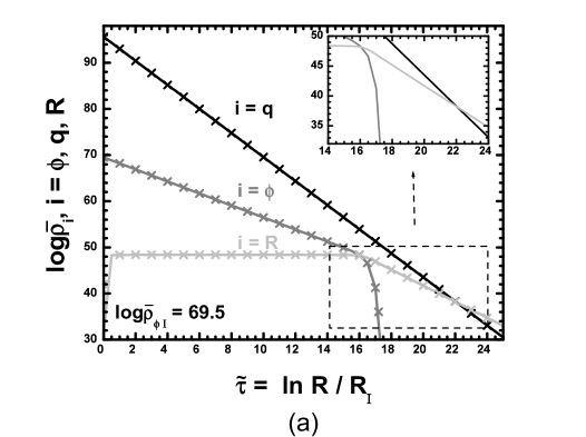
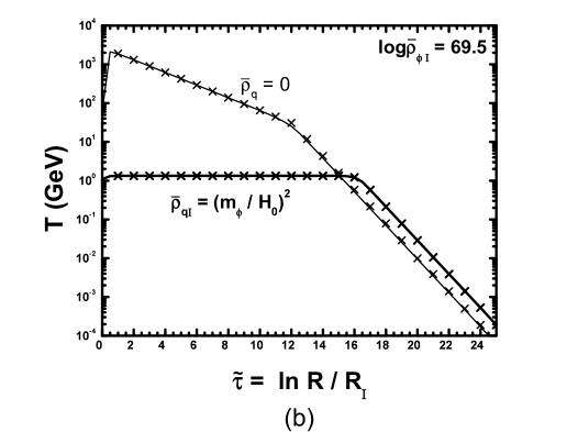
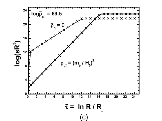
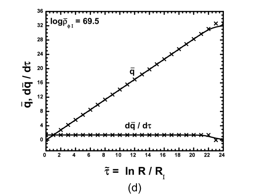
Figure 1: The evolution as a function of $\tilde{\tau}$$\iota$ for $m_{\phi}=10^{6}~{}{\rm GeV}$, $T_{\phi}=30~{}{\rm GeV}$ and $\log{\mbox{$\bar{\rho}_{\phi_{\rm I}}$}}=69.5$ of the quantities: $\log\bar{\rho}_{i}$ with $i=q$ (black line and crosses), $i=\phi$ (gray line and crosses), $i=R$ (light gray line and crosses) (a), $T$ for ${\mbox{$\bar{\rho}_{q_{\rm I}}$}}=(m_{\phi}/H_{0})^{2}~{}[{\mbox{$\bar{\rho}_{q}$}}=0]$ (bold [thin] line and crosses) (b), $\log(sR^{3})$ for ${\mbox{$\bar{\rho}_{q_{\rm I}}$}}=(m_{\phi}/H_{0})^{2}~{}[{\mbox{$\bar{\rho}_{q}$}}=0]$ (bold [thin] line and crosses) (c), $\bar{q}$ and ${\mbox{$\bar{q}$}}^{\prime}$ (d). The solid lines [crosses] are obtained by our numerical code [semi-analytical expressions].

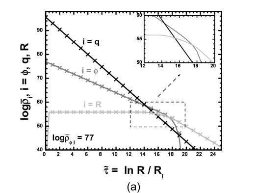
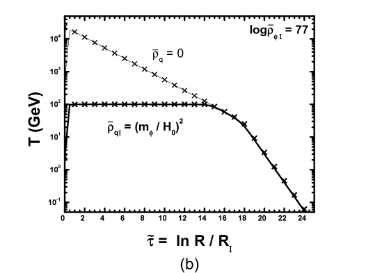
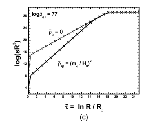
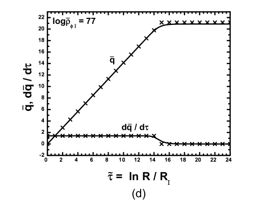
Figure 2: The same as in fig. 1 but with $\log{\mbox{$\bar{\rho}_{\phi_{\rm I}}$}}=77$.

4.1 COMPLETE VERSUS PARTIAL DOMINATION OF KINATION

The two kinds of $q$-domination, $q$-TD and $q$-PD, described in sec. 2.4.3 are explored in fig. 1 and fig. 2, respectively. Namely, in fig. 1 [fig. 2], we illustrate the cosmological evolution of the various quantities as a function of $\tilde{\tau}$$\iota$ for $m_{\phi}=10^{6}~{}{\rm GeV}$, $T_{\phi}=30~{}{\rm GeV}$ and $\log{\mbox{$\bar{\rho}_{\phi_{\rm I}}$}}=69.5$ [$\log{\mbox{$\bar{\rho}_{\phi_{\rm I}}$}}=77$] (the inputs and some key outputs of our running are listed in the first [fourth] column of table 2). We present solid lines [crosses] which are obtained by our numerical code described in sec. 2.2 [semi-analytical expressions as we explain in secs. 3.1 and 3.2] so as we can check the accuracy of the formulas derived in sec. 2.4. In particular, we design:

$\bullet$ $\log\bar{\rho}_{i}$ with $i=q$ (black line and crosses), $i=\phi$ (gray line and crosses), $i=R$ (light gray line and crosses) versus $\tilde{\tau}$$\iota$, in figs. 1-(a) and 2-(a). In both cases we observe that ${\mbox{$\bar{\rho}$}}_{q}$ decreases more steeply than ${\mbox{$\bar{\rho}$}}_{\phi}$, and ${\mbox{$\bar{\rho}$}}_{{}_{\rm R}}$ remains predominantly constant. On the other hand, in fig. 1-(a) [2-(a)], we observe that: (i) we obtain 2 [3] intersections of the various lines, (ii) the hierarchy of the various intersection points is ${\mbox{$\leavevmode\hbox{\normalsize$\tilde{\tau}$\kern-5.0pt$\iota$}_{{}_{\phi\rm R}}$}}<{\mbox{$\leavevmode\hbox{\normalsize$\tilde{\tau}$\kern-5.0pt$\iota$}_{{}_{\rm KR}}$}}$ [${\mbox{$\leavevmode\hbox{\normalsize$\tilde{\tau}$\kern-5.0pt$\iota$}_{{}_{\rm K\phi}}$}}<{\mbox{$\leavevmode\hbox{\normalsize$\tilde{\tau}$\kern-5.0pt$\iota$}_{{}_{\rm KR}}$}}<{\mbox{$\leavevmode\hbox{\normalsize$\tilde{\tau}$\kern-5.0pt$\iota$}_{{}_{\phi\rm R}}$}}$], (iii) at the point of the last intersection (${\mbox{$\leavevmode\hbox{\normalsize$\tilde{\tau}$\kern-5.0pt$\iota$}_{{}_{\rm RD}}$}}={\mbox{$\leavevmode\hbox{\normalsize$\tilde{\tau}$\kern-5.0pt$\iota$}_{{}_{\rm KR}}$}}$ [${\mbox{$\leavevmode\hbox{\normalsize$\tilde{\tau}$\kern-5.0pt$\iota$}_{{}_{\rm RD}}$}}={\mbox{$\leavevmode\hbox{\normalsize$\tilde{\tau}$\kern-5.0pt$\iota$}_{{}_{\phi\rm R}}$}}$]), we obtain $({\mbox{$\bar{\rho}$}}_{q}/{\mbox{$\bar{\rho}$}}_{\phi})({\mbox{$\leavevmode\hbox{\normalsize$\tilde{\tau}$\kern-5.0pt$\iota$}_{{}_{\rm RD}}$}})\gg 1$ [$({\mbox{$\bar{\rho}$}}_{q}/{\mbox{$\bar{\rho}$}}_{\phi})({\mbox{$\leavevmode\hbox{\normalsize$\tilde{\tau}$\kern-5.0pt$\iota$}_{{}_{\rm RD}}$}})\ll 1$] as expected from eq. (36).

$\bullet$ $T$ versus $\tilde{\tau}$$\iota$, for ${\mbox{$\bar{\rho}_{q_{\rm I}}$}}=(m_{\phi}/H_{0})^{2}~{}[{\mbox{$\bar{\rho}_{q}$}}=0]$ (bold [thin] line and crosses) in figs. 1-(b) and 2-(b) (obviously the thin lines correspond to a LRS with the same $\bar{\rho}_{\phi_{\rm I}}$). In both cases we observe that $T$ rapidly takes its maximal plateau value, which is much lower than its maximal value obtained in the LRS – see eqs. (41) and (31). However, in fig. 1-(b) the transition from the $\rho_{{}_{\rm R}}<\rho_{\phi}$ to the $\rho_{{}_{\rm R}}>\rho_{\phi}$ phase, takes place at ${\mbox{$\leavevmode\hbox{\normalsize$\tilde{\tau}$\kern-5.0pt$\iota$}_{{}_{\phi\rm R}}$}}\simeq 16.08$ [${\mbox{$\leavevmode\hbox{\normalsize$\tilde{\tau}$\kern-5.0pt$\iota$}_{{}_{\rm RH}}$}}\simeq 12.06$] (where a corner [kink] is observed on the bold [thin] line), whereas in fig. 2-(b), the same transition takes place practically at a common point ${\mbox{$\leavevmode\hbox{\normalsize$\tilde{\tau}$\kern-5.0pt$\iota$}_{{}_{\phi\rm R}}$}}\simeq 17.47$ for both the LRS and KRS where a slight kink is observed on both lines. This is expected since in fig. 2-(b) we obtain $q$-PD and so, for $\leavevmode\hbox{\normalsize$\tilde{\tau}$\kern-5.0pt$\iota$}>{\mbox{$\leavevmode\hbox{\normalsize$\tilde{\tau}$\kern-5.0pt$\iota$}_{{}_{\rm K\phi}}$}}=14.3$, the KRS and LRS give similar results.

$\bullet$ $\log(sR^{3})$ versus $\tilde{\tau}$$\iota$, for ${\mbox{$\bar{\rho}_{q_{\rm I}}$}}=(m_{\phi}/H_{0})^{2}~{}[{\mbox{$\bar{\rho}_{q}$}}=0]$ (bold [thin] line and crosses) in figs. 1-(c) and 2-(c). In both cases we observe that the initial entropy $(sR^{3})(0)$ is much lower in the KRS than in the LRS. At the points where we observe a corner or a kink on the lines of fig. 1-(b) [figs. 2-(b)], a plateau, which represents the transition to the isentropic expansion, appears in fig. 1-(c) [figs. 2-(c)]. The appearance of the plateau observed on the bold and thin lines for $q$-TD – fig. 1-(c) – occurs at different points (${\mbox{$\leavevmode\hbox{\normalsize$\tilde{\tau}$\kern-5.0pt$\iota$}_{{}_{\phi\rm R}}$}}\simeq 16.08$ and ${\mbox{$\leavevmode\hbox{\normalsize$\tilde{\tau}$\kern-5.0pt$\iota$}_{{}_{\rm RH}}$}}\simeq 12.06$), whereas for $q$-PD – fig. 2-(c) – the same effect is realized at a common point since ${\mbox{$\leavevmode\hbox{\normalsize$\tilde{\tau}$\kern-5.0pt$\iota$}_{{}_{\phi\rm R}}$}}\simeq 17.5$ and ${\mbox{$\leavevmode\hbox{\normalsize$\tilde{\tau}$\kern-5.0pt$\iota$}_{{}_{\rm RH}}$}}\simeq 17.82$. This is expected, since for $\leavevmode\hbox{\normalsize$\tilde{\tau}$\kern-5.0pt$\iota$}>{\mbox{$\leavevmode\hbox{\normalsize$\tilde{\tau}$\kern-5.0pt$\iota$}_{{}_{\rm K\phi}}$}}=14.3$ and $q$-PD, the KRS almost coincides to LRS (with the same $\bar{\rho}_{\phi_{\rm I}}$).

$\bullet$ $q$ and $q^{\prime}$ versus $\tilde{\tau}$$\iota$, in figs. 1-(d) and 2-(d). In both cases we observe the period of the $q$-evolution according to eq. (44) with constant inclination ($\sqrt{2}$) and the onset of the frozen field dominated phase ($q^{\prime}=0$). However, we observe that the frozen field phase commences much earlier in fig. 2-(d) (for $q$-PD) and $q$ takes a value lower than the one in fig. 1-(d) (for $q$-TD) – see eqs. (46) and (50).

4.2 EQUILIBRIUM VERSUS NON-EQUILIBRIUM PRODUCTION

FIGS.	1, 3-${\sf(a_{1})}$	3-${\sf(a_{2})}$	3-${\sf(b_{1})}$	2, 3-${\sf(b_{2})}$
INPUT PARAMETERS
$\lambda=0.5,~{}m_{\phi}=10^{6}~{}{\rm GeV},~{}T_{\phi}=30~{}{\rm GeV},~{}m_{\chi}=350~{}{\rm GeV}$
$\log{\mbox{$\bar{\rho}_{\phi_{\rm I}}$}}$	$69.5$	$73.82$	$74.3$	$77$
${\mbox{$\langle\sigma v\rangle$}}~{}({\rm GeV}^{-2})$	$10^{-10}$	$10^{-10}$	$2\times 10^{-9}$	$1.8\times 10^{-9}$
$N_{\chi}$	$10^{-6}$	$0$	$0$	$0$
$\bar{V}_{0}$	$7\times 10^{11}$	$2.25\times 10^{9}$	$1.18\times 10^{9}$	$5.5\times 10^{7}$
OUTPUT PARAMETERS
$T_{\rm PL}~{}({\rm GeV})$	1.3	16.05	21.1	100
$\leavevmode\hbox{\normalsize$\tilde{\tau}$\kern-5.0pt$\iota$}_{{}_{\rm K\phi}}$	$-$	$-$	$-$	14.3
${\mbox{$T_{{\rm K\phi}}$}}~{}({\rm GeV})$	$-$	$-$	$-$	94.7
$\leavevmode\hbox{\normalsize$\tilde{\tau}$\kern-5.0pt$\iota$}_{{}_{\phi\rm R}}$	16.08	16.09	16.1	17.5
${\mbox{$T_{\phi{\rm R}}$}}~{}({\rm GeV})$	1.3	16.05	21.1	100
$\leavevmode\hbox{\normalsize$\tilde{\tau}$\kern-5.0pt$\iota$}_{{}_{\rm KR}}$	22.1	17.1	16.6	15.5
${\mbox{$T_{{\rm KR}}$}}~{}({\rm GeV})$	0.0035	6.31	13.9	70.2
${\mbox{$\bar{\rho}_{q_{\rm I}}$}}/{\mbox{$\bar{\rho}_{\phi_{\rm I}}$}}$	$1.3\times 10^{26}$	$6.4\times 10^{21}$	$2\times 10^{21}$	$4.2\times 10^{18}$
$({\mbox{$\bar{\rho}$}}_{q}/{\mbox{$\bar{\rho}$}}_{\phi})({\mbox{$\leavevmode\hbox{\normalsize$\tilde{\tau}$\kern-5.0pt$\iota$}_{{}_{\rm RD}}$}})$	$2.5\times 10^{22}$	$1.2\times 10^{6}$	$11.84$	$2\times 10^{-4}$
$\Omega_{q}({\mbox{$\leavevmode\hbox{\normalsize$\tau$\kern-5.0pt$\iota$}_{{}_{\rm NS}}$}})$	0.01	$3\times 10^{-9}$	$5.6\times 10^{-10}$	$7\times 10^{-15}$
$\leavevmode\hbox{\normalsize$\tilde{\tau}$\kern-5.0pt$\iota$}_{\ast}$	15.25	15.7	$15.8$	$15.3$
$x^{-1}_{*}$	265	22.7	$17.45$	$4.6$
$(f_{\chi}^{\rm eq}/f_{\chi}^{nN})({\mbox{$\leavevmode\hbox{\normalsize$\tilde{\tau}$\kern-5.0pt$\iota$}_{\ast}$}})$	$0$	12.6	0.0016	$5\times 10^{-9}$
$\leavevmode\hbox{\normalsize$\tilde{\tau}$\kern-5.0pt$\iota$}_{{}_{\rm F}}$	$-$	$-$	16.5	18.5
$x^{-1}_{{}_{\rm F}}$	$-$	$-$	23.45	23.86
$\Omega_{\chi}h^{2}$	0.11	0.11	0.11	0.11
$\Omega_{\chi}h^{2}|_{\rm SC}$	1.87	1.87	0.11	0.12
$\Omega_{\chi}h^{2}|_{{\mbox{$\bar{\rho}_{q}$}}=0}$	1.78	1.78	0.1	0.11
$\Omega_{\chi}h^{2}|_{{\mbox{$\bar{\rho}_{\phi}$}}=0}$	979	2.86	0.12	0.12

Table 2: Input and output parameters for the four examples illustrated in figs. 3-${\sf(a_{1})},~{}{\sf(a_{2})},~{}{\sf(b_{1})}$ and ${\sf(b_{2})}$ (see also figs. 1 and 2).

The various kinds of $\chi$-production encountered in the KRS, are explored in fig. 3. In this, we check also the accuracy of our semi-analytical expressions (which describe the $f_{\chi}$ and $f_{\chi}^{\rm eq}$ evolution), displaying by bold solid lines [crosses] the results obtained by our numerical code (see sec. 2.2) [semi-analytical expressions (see secs. 3.2 and 3.1)]. The thin crosses are obtained by inserting $T$ (given as we describe in secs. 3.2 and 3.1) into eq. (8).

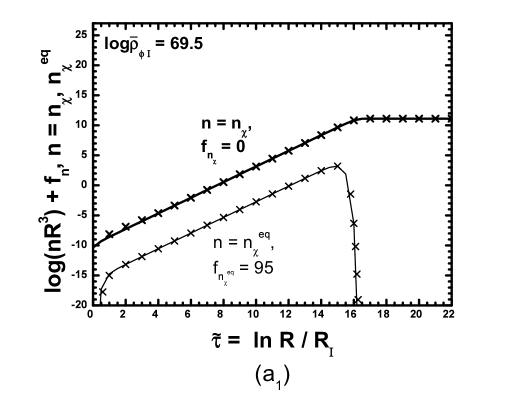
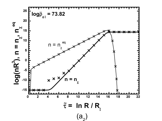
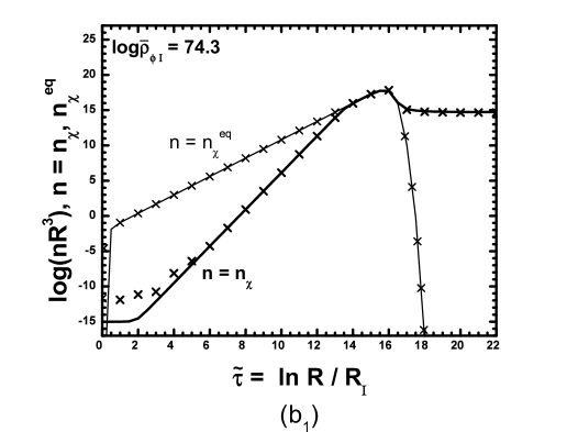
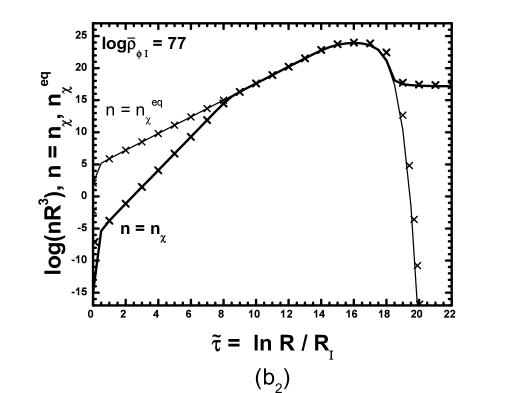
Figure 3: The evolution as a function of $\tilde{\tau}$$\iota$ of the quantities $\log(n_{\chi}R^{3})$ (bold line and crosses) and $\log(n^{\rm eq}_{\chi}R^{3})+f_{n^{\rm eq}_{\chi}}$ (thin line and crosses) for $m_{\phi}=10^{6}~{}{\rm GeV},~{}T_{\phi}=30~{}{\rm GeV}$ and: ${\sf(a_{1})}$ $\log{\mbox{$\bar{\rho}_{\phi_{\rm I}}$}}=69.5,~{}N_{\chi}=10^{-6}$ and ${\mbox{$\langle\sigma v\rangle$}}=10^{-10}~{}{\rm GeV}^{-2}$, ${\sf(a_{2})}$ $\log{\mbox{$\bar{\rho}_{\phi_{\rm I}}$}}=73.82,~{}N_{\chi}=0$ and ${\mbox{$\langle\sigma v\rangle$}}=10^{-10}~{}{\rm GeV}^{-2}$, ${\sf(b_{1})}$ $\log{\mbox{$\bar{\rho}_{\phi_{\rm I}}$}}=74.3,~{}N_{\chi}=0$ and ${\mbox{$\langle\sigma v\rangle$}}=2\times 10^{-9}~{}{\rm GeV}^{-2}$ and ${\sf(b_{2})}$ $\log{\mbox{$\bar{\rho}_{\phi_{\rm I}}$}}=77,~{}N_{\chi}=0$ and ${\mbox{$\langle\sigma v\rangle$}}=1.8\times 10^{-9}~{}{\rm GeV}^{-2}$ ($f_{n^{\rm eq}_{\chi}}=95$ in the case ${\sf(a_{1})}$ and $f_{n^{\rm eq}_{\chi}}=0$ elsewhere). The solid lines [crosses] are obtained by our numerical code [semi-analytical expressions]. In all cases, we extract $\Omega_{\chi}h^{2}=0.11$.

The inputs parameters and some key outputs for the four examples illustrated in fig. 3 are listed in table 2. In particular, we present $\tilde{\tau}$$\iota$’s and the corresponding $T$’s of the possible intersections between the various energy-densities. Comparing the relevant results, we observe that as $\bar{\rho}_{\phi_{\rm I}}$ increases, ${\mbox{$\bar{\rho}_{q_{\rm I}}$}}/{\mbox{$\bar{\rho}_{\phi_{\rm I}}$}}$ decreases (note that eq. (21) remains always valid), and so, $({\mbox{$\bar{\rho}$}}_{q}/{\mbox{$\bar{\rho}$}}_{\phi})({\mbox{$\leavevmode\hbox{\normalsize$\tilde{\tau}$\kern-5.0pt$\iota$}_{{}_{\rm RD}}$}})$ and $\Omega_{q}({\mbox{$\leavevmode\hbox{\normalsize$\tau$\kern-5.0pt$\iota$}_{{}_{\rm NS}}$}})$ decrease too. At the same time, $\leavevmode\hbox{\normalsize$\tilde{\tau}$\kern-5.0pt$\iota$}_{{}_{\phi\rm R}}$ eventually approaches $\leavevmode\hbox{\normalsize$\tilde{\tau}$\kern-5.0pt$\iota$}_{{}_{\rm KR}}$ and becomes larger than this for $\log{\mbox{$\bar{\rho}_{\phi_{\rm I}}$}}=77$, where $q$-PD is achieved (in the other cases we have $q$-TD). In the same table we provide $\leavevmode\hbox{\normalsize$\tilde{\tau}$\kern-5.0pt$\iota$}_{\ast}$’s, derived from the maximalization of the intergrand in eq. (56), and we applied the criterion of eq. (57). In the case of EP, $\leavevmode\hbox{\normalsize$\tilde{\tau}$\kern-5.0pt$\iota$}_{{}_{\rm F}}$’s and $x_{{}_{\rm F}}$’s derived from eq. (60) are also given. In all cases, we extract $\Omega_{\chi}h^{2}=0.11$ and we show the resultant $\Omega_{\chi}h^{2}$ in several other related scenaria (see also sec. 4.4).

We design the evolution of $\log f_{\chi}$ (bold line and crosses) and $\log f_{\chi}^{\rm eq}+f_{n^{\rm eq}_{\chi}}$ (thin line and crosses) as a function of $\tilde{\tau}$$\iota$ for $m_{\phi}=10^{6}~{}{\rm GeV},~{}T_{\phi}=30~{}{\rm GeV}$ and:

$\bullet$ $\log{\mbox{$\bar{\rho}_{\phi_{\rm I}}$}}=69.5,~{}N_{\chi}=10^{-6}$ ($f_{n^{\rm eq}_{\chi}}=95$) and ${\mbox{$\langle\sigma v\rangle$}}=10^{-10}~{}{\rm GeV}^{-2}$ in fig. 3-${\sf(a_{1})}$. In this case, we obtain $q$-TD (the evolution of the various energy densities is presented in fig. 1-(a)). The quantity $n^{\rm eq}_{\chi}$ turns out to be strongly suppressed due to very low $T_{\rm PL}\ll m_{\chi}/20$ and so, we obtain $f_{\chi}\gg f^{\rm eq}_{\chi}$ for any $\leavevmode\hbox{\normalsize$\tilde{\tau}$\kern-5.0pt$\iota$}<25$. This is a typical example of non-EPI, where the presence of $N_{\chi}>0$ is indispensable so as to obtain interesting $\Omega_{\chi}h^{2}$. Fixing $N_{\chi}=10^{-6}$ and adjusting $\bar{\rho}_{\phi_{\rm I}}$, we achieve $\Omega_{\chi}h^{2}=0.11$. The bold crosses are derived by solving numerically eq. (53) for $\leavevmode\hbox{\normalsize$\tilde{\tau}$\kern-5.0pt$\iota$}<{\mbox{$\leavevmode\hbox{\normalsize$\tilde{\tau}$\kern-5.0pt$\iota$}_{{}_{\rm RD}}$}}$ (since $\langle\sigma v\rangle$ is rather low, eq. (54) is also valid) and from eq. (66) for ${\mbox{$\leavevmode\hbox{\normalsize$\tilde{\tau}$\kern-5.0pt$\iota$}_{{}_{\rm RD}}$}}<\leavevmode\hbox{\normalsize$\tilde{\tau}$\kern-5.0pt$\iota$}<{\mbox{$\leavevmode\hbox{\normalsize$\tilde{\tau}$\kern-5.0pt$\iota$}_{{}_{\rm f}}$}}$. The constant-$f_{\chi}$ phase commences at $\leavevmode\hbox{\normalsize$\tilde{\tau}$\kern-5.0pt$\iota$}\simeq 16.1$, where the integrand of $f_{\chi}^{N}$ in eq. (54) reaches its maximum.

$\bullet$ $\log{\mbox{$\bar{\rho}_{\phi_{\rm I}}$}}=73.82,~{}N_{\chi}=0$ ($f_{n^{\rm eq}_{\chi}}=0$) and ${\mbox{$\langle\sigma v\rangle$}}=10^{-10}~{}{\rm GeV}^{-2}$ in fig. 3-${\sf(a_{2})}$. In contrast with the previous case, we obtain a less efficient $q$-TD and so, $T_{\rm PL}$ turns out to be significantly larger ($T_{\rm PL}\sim m_{\chi}/20$). This is a typical example of non-EPII since at ${\mbox{$\leavevmode\hbox{\normalsize$\tilde{\tau}$\kern-5.0pt$\iota$}_{\ast}$}}\simeq 15.7$, we get $f_{\chi}<f^{\rm eq}_{\chi}$. By adjusting $\bar{\rho}_{\phi_{\rm I}}$, we achieve $\Omega_{\chi}h^{2}=0.11$. The bold crosses are extracted from eq. (56) for $\leavevmode\hbox{\normalsize$\tilde{\tau}$\kern-5.0pt$\iota$}<{\mbox{$\leavevmode\hbox{\normalsize$\tilde{\tau}$\kern-5.0pt$\iota$}_{{}_{\rm RD}}$}}$ and from eq. (66) for ${\mbox{$\leavevmode\hbox{\normalsize$\tilde{\tau}$\kern-5.0pt$\iota$}_{{}_{\rm RD}}$}}<\leavevmode\hbox{\normalsize$\tilde{\tau}$\kern-5.0pt$\iota$}<{\mbox{$\leavevmode\hbox{\normalsize$\tilde{\tau}$\kern-5.0pt$\iota$}_{{}_{\rm f}}$}}$. The onset of the constant-$f_{\chi}$ phase occurs at ${\mbox{$\leavevmode\hbox{\normalsize$\tilde{\tau}$\kern-5.0pt$\iota$}_{\ast}$}}\simeq 15.7$.

$\bullet$ $\log{\mbox{$\bar{\rho}_{\phi_{\rm I}}$}}=74.3,~{}N_{\chi}=0$ ($f_{n^{\rm eq}_{\chi}}=0$) and ${\mbox{$\langle\sigma v\rangle$}}=2\times 10^{-9}~{}{\rm GeV}^{-2}$ in fig. 3-${\sf(b_{1})}$. In this case, we obtain a weak (since $\leavevmode\hbox{\normalsize$\tilde{\tau}$\kern-5.0pt$\iota$}_{{}_{\phi\rm R}}$ is very close to $\leavevmode\hbox{\normalsize$\tilde{\tau}$\kern-5.0pt$\iota$}_{{}_{\rm KR}}$, as shown in table 1) $q$-TD with $T_{\rm PL}>T_{\rm F}$. This is a typical example of EP before the onset of RD era, since for ${\mbox{$\leavevmode\hbox{\normalsize$\tilde{\tau}$\kern-5.0pt$\iota$}_{\ast}$}}\sim 15.8$, we get $f_{\chi}>f^{\rm eq}_{\chi}$ and ${\mbox{$\leavevmode\hbox{\normalsize$\tilde{\tau}$\kern-5.0pt$\iota$}_{{}_{\rm F}}$}}<{\mbox{$\leavevmode\hbox{\normalsize$\tilde{\tau}$\kern-5.0pt$\iota$}_{{}_{\rm RD}}$}}={\mbox{$\leavevmode\hbox{\normalsize$\tilde{\tau}$\kern-5.0pt$\iota$}_{{}_{\rm KR}}$}}$. $\Omega_{\chi}h^{2}=0.11$ is achieved by adjusting $\langle\sigma v\rangle$. The bold crosses are extracted by solving numerically eq. (16) after substituting in it $H$ and $T$ as we describe in secs. 3.2 and 3.1. They could be, also, derived from eq. (62) for ${\mbox{$\leavevmode\hbox{\normalsize$\tilde{\tau}$\kern-5.0pt$\iota$}_{{}_{\rm F}}$}}<\leavevmode\hbox{\normalsize$\tilde{\tau}$\kern-5.0pt$\iota$}<{\mbox{$\leavevmode\hbox{\normalsize$\tilde{\tau}$\kern-5.0pt$\iota$}_{{}_{\rm RD}}$}}$ and from eq. (66) for ${\mbox{$\leavevmode\hbox{\normalsize$\tilde{\tau}$\kern-5.0pt$\iota$}_{{}_{\rm RD}}$}}<\leavevmode\hbox{\normalsize$\tilde{\tau}$\kern-5.0pt$\iota$}<{\mbox{$\leavevmode\hbox{\normalsize$\tilde{\tau}$\kern-5.0pt$\iota$}_{{}_{\rm f}}$}}$.

FIG.	RANGES OF THE LOWER $x$-AXIS PARAMETERS				$\chi$-PRO-
	$N_{\chi}=0$	$N_{\chi}=10^{-7}$	$N_{\chi}=10^{-6}$	$N_{\chi}=10^{-5}$	DUCTION
4-${\sf(a_{1})}$	$-$	$68.56-73.39$	$68.56-73.56$	$68.56-73.74$	non-EPI
	$73.75-73.93$	$-$	$-$	$-$	non-EPII
	$73.94-74$	$73.4-74$	$73.57-74$	$73.75-74$	EP
4-${\sf(a_{2})}$	$-$	$68.56-73.44$	$68.56-73.53$	$68.56-73.72$	non-EPI
	$73.5-73.6$	$-$	$-$	$-$	non-EPII
	$73.61-74.5$	$73.45-74.5$	$73.54-74.5$	$73.73-74.5$	EP
4-${\sf(b_{1})}$	$-$	$1-3.17$	$(-0.9)-3$	$(-0.9)-0.698$	non-EPI
	$-$	$3.18-3.28$	$-$	$-$	EP
	$3.54-3.69$	$3.29-3.69$	$-$	$-$	non-EPII
4-${\sf(b_{2})}$	$-$	$1-3.17$	$(-0.9)-3$	$(-0.9)-0.698$	non-EPI
	$-$	$3.18-3.28$	$-$	$-$	EP
	$3.4-3.54$	$3.29-3.54$	$-$	$-$	non-EPII
4-${\sf(c_{1})}$	$-$	$5-6.5$	$5.8-6.8$	$6.5-6.8$	non-EPI
	$3.88-4.1$	$-$	$-$	$-$	non-EPII
4-${\sf(c_{2})}$	$3-4$	$3-4.2$	$3-4$	3-3.7	EP
	$-$	$4.3-6.5$	$5.7-6.8$	$6.5-6.8$	non-EPI
	$4-4.3$	$-$	$-$	$-$	non-EPII

Table 3: The type of $\chi$-production for various ranges of the lower $x$-axis parameters and $N_{\chi}$’s in fig. 4.

$\bullet$ $\log{\mbox{$\bar{\rho}_{\phi_{\rm I}}$}}=77,~{}N_{\chi}=0$ ($f_{n^{\rm eq}_{\chi}}=0$) and ${\mbox{$\langle\sigma v\rangle$}}=1.8\times 10^{-9}~{}{\rm GeV}^{-2}$ in fig. 3-${\sf(b_{2})}$. In this case, we obtain $q$-PD (the evolution of the various energy densities is presented in fig 2-(a)) and $T_{\rm PL}\gg T_{\rm F}$. This is a typical example of EP after the onset of the RD era, since for ${\mbox{$\leavevmode\hbox{\normalsize$\tilde{\tau}$\kern-5.0pt$\iota$}_{\ast}$}}\simeq 15.3$ we get $f_{\chi}>f^{\rm eq}_{\chi}$, and ${\mbox{$\leavevmode\hbox{\normalsize$\tilde{\tau}$\kern-5.0pt$\iota$}_{{}_{\rm F}}$}}\simeq 18.5>{\mbox{$\leavevmode\hbox{\normalsize$\tilde{\tau}$\kern-5.0pt$\iota$}_{{}_{\rm RD}}$}}={\mbox{$\leavevmode\hbox{\normalsize$\tilde{\tau}$\kern-5.0pt$\iota$}_{{}_{\phi\rm R}}$}}\simeq 17.5$. $\Omega_{\chi}h^{2}=0.11$ is achieved by adjusting $\langle\sigma v\rangle$. The bold crosses are extracted similarly to the previous case. They could be also derived from eq. (66) for ${\mbox{$\leavevmode\hbox{\normalsize$\tilde{\tau}$\kern-5.0pt$\iota$}_{{}_{\rm F}}$}}<\leavevmode\hbox{\normalsize$\tilde{\tau}$\kern-5.0pt$\iota$}<{\mbox{$\leavevmode\hbox{\normalsize$\tilde{\tau}$\kern-5.0pt$\iota$}_{{}_{\rm f}}$}}$.

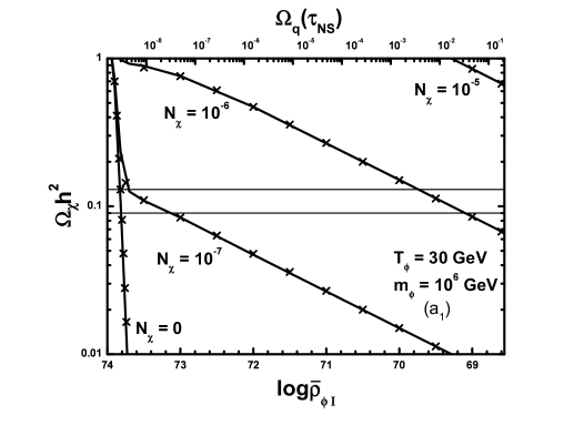
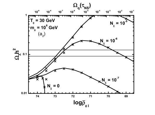
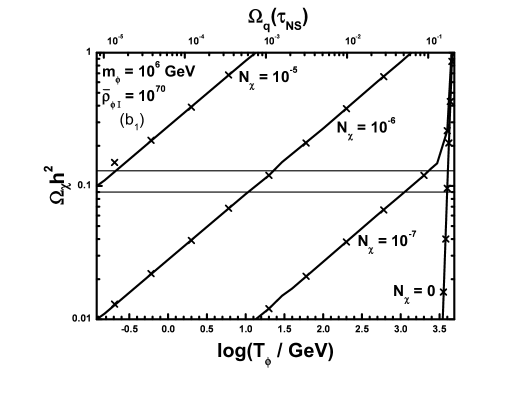
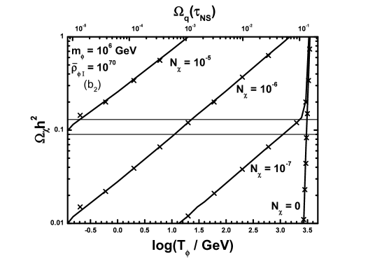
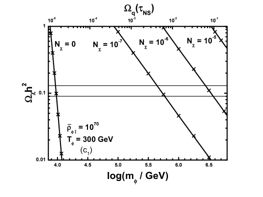
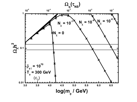
Figure 4: $\Omega_{\chi}h^{2}$ versus $\log{\mbox{$\bar{\rho}_{\phi_{\rm I}}$}}~{}{\sf(a_{1},a_{2})}$, $\log T_{\phi}~{}{\sf(b_{1},b_{2})}$ and $\log m_{\phi}~{}{\sf(c_{1},c_{2})}$ for fixed (indicated in the graphs) $T_{\phi}$ and $m_{\phi}$, $\bar{\rho}_{\phi_{\rm I}}$ and $m_{\phi}$, $\bar{\rho}_{\phi_{\rm I}}$ and $T_{\phi}$ correspondingly, and various $N_{\chi}$’s indicated on the curves. We take $m_{\tilde{\chi}}=350~{}{\rm GeV}$ and $\langle\sigma v\rangle=10^{-10}~{}{\rm GeV^{-2}}~{}[\langle\sigma v\rangle=10^{-8}~{}{\rm GeV^{-2}}]~{}{\sf(a_{1},b_{1},c_{1}~{}[a_{2},b_{2},c_{2}])}$. The solid lines [crosses] are obtained by our numerical code [semi-analytical expressions]. The CDM bounds of eq. (2) are, also, depicted by the two thin lines.

4.3 $\Omega_{\chi}h^{2}$ AS A FUNCTION OF THE FREE PARAMETERS

Varying the free parameters, useful conclusions can be inferred for the behavior of $\Omega_{\chi}h^{2}$ and the regions where each ${\chi}$-production mechanism can be activated. In addition, a final test of our semi-analytical approach can be presented by comparing its results for $\Omega_{\chi}h^{2}$ with those obtained by solving numerically the problem. We focus on $q$-TD, since the results for $q$-PD are similar to those obtained in the LRS (see secs. 2.4.2 and ref. [14]).

Our results are displayed in figs. 4 and 5. The solid lines are drawn from the results of the numerical integration of eqs. (13)-(16), whereas crosses are obtained by solving numerically eq. (16) as we describe in secs. 3.1 and 3.2 (comments on the validity of eqs. (54), (56) and (62) are given, too). The running of $f_{\chi}$ after the onset of the RD era – see eqs. (62) and (66) – although crucial for the final result (especially for weak $q$-TD) does not alter the behaviour of the solution as a function of the free parameters. The type of ${\chi}$-production for the lower $x$-axis parameters and the various $N_{\chi}$’s used in fig. 4 is presented in table 3. From this and taking into account the obtained $T_{\rm PL}$’s in each case (see below), we can induce that non-EP (non-EPI [non-EPII] for $N_{\chi}\neq 0$ [$N_{\chi}\sim 0$]) is dominant for $T_{\rm PL}\lesssim m_{\chi}/20$, whereas EP is activated for $T_{\rm PL}>m_{\chi}/20$.

In figs. 4-${\sf(a_{1},b_{1},c_{1})}$ [figs. 4-${\sf(a_{2},b_{2},c_{2})}$], we take $m_{\chi}=350~{}{\rm GeV}$ and $\langle\sigma v\rangle=10^{-10}~{}{\rm GeV^{-2}}$ [$\langle\sigma v\rangle=10^{-8}~{}{\rm GeV^{-2}}$]. We design $\Omega_{\chi}h^{2}$ versus:

$\bullet$ $\log{\mbox{$\bar{\rho}_{\phi_{\rm I}}$}}$ (or $\Omega_{q}({\mbox{$\leavevmode\hbox{\normalsize$\tau$\kern-5.0pt$\iota$}_{{}_{\rm NS}}$}})$) in fig. 4-${\sf(a_{1})}$ and ${\sf(a_{2})}$ for $T_{\phi}=30~{}{\rm GeV}$, $m_{\phi}=10^{6}~{}{\rm GeV}$ and several $N_{\chi}$’s indicated on the curves. We observe that: (i) $\Omega_{q}({\mbox{$\leavevmode\hbox{\normalsize$\tau$\kern-5.0pt$\iota$}_{{}_{\rm NS}}$}})$ increases as $\bar{\rho}_{\phi_{\rm I}}$ decreases (since ${\mbox{$\bar{\rho}_{q_{\rm I}}$}}/{\mbox{$\bar{\rho}_{\phi_{\rm I}}$}}$ increases too) and so, a lower bound on $\bar{\rho}_{\phi_{\rm I}}$ can be derived from eq. (22a) – note that $T_{\rm PL}$ decreases with $\bar{\rho}_{\phi_{\rm I}}$ (see eq. (41)) and ranges between (0.8 and 24) GeV, (ii) $\Omega_{\chi}h^{2}$ decreases with $\bar{\rho}_{\phi_{\rm I}}$ in fig. 4-${\sf(a_{1})}$ ($\langle\sigma v\rangle=10^{-10}~{}{\rm GeV^{-2}}$) whereas it increases as $\bar{\rho}_{\phi_{\rm I}}$ decreases (for large $\bar{\rho}_{\phi_{\rm I}}$’s) and decreases with $\bar{\rho}_{\phi_{\rm I}}$ (for low $\bar{\rho}_{\phi_{\rm I}}$’s) in fig. 4-${\sf(a_{2})}$ ($\langle\sigma v\rangle=10^{-8}~{}{\rm GeV^{-2}}$). The last observation can be explained as follows: $f_{\chi}$ can be mostly given by solving numerically eq. (53) – see table 3. $f_{\chi}$ increases with $\bar{\rho}_{\phi_{\rm I}}$ and so, when $\langle\sigma v\rangle$ is large enough ($\sim 10^{-8}~{}{\rm GeV}^{-2}$) the first term in the r.h.s of eq. (53) becomes comparable to the second one and the solution of eq. (53) can be exclusively realized numerically. For lower $\bar{\rho}_{\phi_{\rm I}}$’s, eq. (54) can be used and so, $f_{\chi}$ decreases with $\bar{\rho}_{\phi_{\rm I}}$. The latter behaviour is dominant for low ${\mbox{$\langle\sigma v\rangle$}}\sim 10^{-10}~{}{\rm GeV^{-2}}$ as in fig. 4-${\sf(a_{1})}$.

$\bullet$ $\log T_{\phi}$ (or $\Omega_{q}({\mbox{$\leavevmode\hbox{\normalsize$\tau$\kern-5.0pt$\iota$}_{{}_{\rm NS}}$}})$) in fig. 4-${\sf(b_{1})}$ and ${\sf(b_{2})}$ for $\log{\mbox{$\bar{\rho}_{\phi_{\rm I}}$}}=70$, $m_{\phi}=10^{6}~{}{\rm GeV}$ and several $N_{\chi}$’s indicated on the curves. We observe that: (i) $\Omega_{q}({\mbox{$\leavevmode\hbox{\normalsize$\tau$\kern-5.0pt$\iota$}_{{}_{\rm NS}}$}})$ increases with $T_{\phi}$ (or $\Gamma_{\phi}$) since $\phi$ decays more rapidly. Therefore, an upper bound on $T_{\phi}$ can be derived from eq. (22a) – note that $T_{\rm PL}$ increases with $T_{\phi}$ (see eq. (41)) and ranges between (0.1 and 23) GeV, (ii) $\Omega_{\chi}h^{2}$ increases with $T_{\phi}$ (or $\Gamma_{\phi}$) and it turns out almost $\langle\sigma v\rangle$-independent for $N_{\chi}\neq 0$ – this is, because $f_{\chi}$ can be mostly given by eq. (54) as shown in table 3, (iii) $\Omega_{\chi}h^{2}$ is $\langle\sigma v\rangle$-dependent and increases rapidly for $N_{\chi}=0$ – this is because $f_{\chi}$ can be extracted from eq. (56) as shown in table 3; $f_{\chi}$ decreases rapidly with $T_{\phi}$ (and $T_{\rm PL}$) due to the exponential suppression of $f^{\rm eq}_{\chi}$.

$\bullet$ $\log m_{\phi}$ (or $\Omega_{q}({\mbox{$\leavevmode\hbox{\normalsize$\tau$\kern-5.0pt$\iota$}_{{}_{\rm NS}}$}})$) in fig. 4-${\sf(c_{1})}$ and ${\sf(c_{2})}$ for $\log m_{\phi}=70$, $T_{\phi}=300~{}{\rm GeV}$ and several $N_{\chi}$’s indicated on the curves. We observe that: (i) $\Omega_{q}({\mbox{$\leavevmode\hbox{\normalsize$\tau$\kern-5.0pt$\iota$}_{{}_{\rm NS}}$}})$ increases with $m_{\phi}$ (since ${\mbox{$\bar{\rho}_{q_{\rm I}}$}}=(m_{\phi}/H_{0})^{2}$ increases too) and so, an upper bound on $m_{\phi}$ can be derived from eq. (22a) – note that $T_{\rm PL}$ decreases as $m_{\phi}$ increases (see eq. (41)) and ranges between (3.5 and 31) GeV, (ii) $\Omega_{\chi}h^{2}$ decreases as $m_{\phi}$ increases for non-EP (see table 3) and increases with $m_{\phi}$ for EP (see fig. 4-${\sf(c_{2})}$ and table 3). This is, because $f_{\chi}$ can be found from eq. (62a) for EP and it increases with $m_{\phi}$ or $H$ (given by eq. (34a)) since $J_{\rm F}$ enters the denominator, whereas $f_{\chi}$ can be derived from eq. (54) [eq. (56)] for non-EPI [non-EPII] and it decreases when $H$ increases.

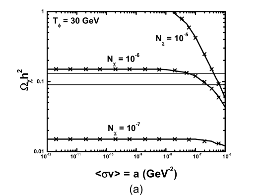
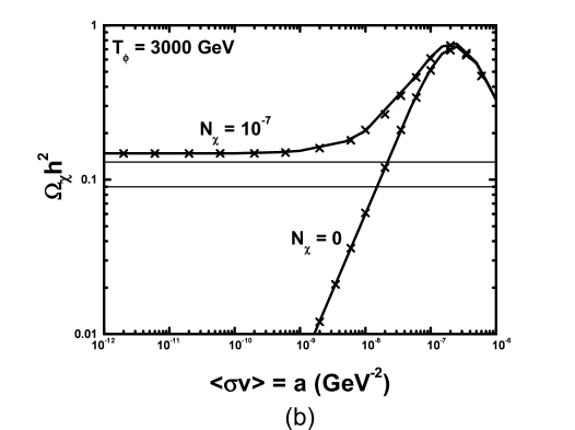
Figure 5: $\Omega_{\chi}h^{2}$ as a function of $\langle\sigma v\rangle=a$ for various $N_{\chi}$’s, indicated on the curves, $m_{\chi}=350~{}{\rm GeV},~{}{\mbox{$\bar{\rho}_{\phi_{\rm I}}$}}=10^{70},~{}m_{\phi}=10^{6}~{}{\rm GeV}$ and $T_{\phi}=30~{}{\rm GeV}~{}[T_{\phi}=3000~{}{\rm GeV}]$ (a [b]). The solid lines [crosses] are obtained by our numerical code [semi-analytical expressions]. The CDM bounds of eq. (2) are, also, depicted by the two thin lines.

The dependence of $\Omega_{\chi}h^{2}$ on $\langle\sigma v\rangle$ can be clearly deduced by fig. 5. We depict $\Omega_{\chi}h^{2}$ as a function of $\langle\sigma v\rangle=a$ for various $N_{\chi}$’s, indicated on the curves, $m_{\chi}=350~{}{\rm GeV},~{}{\mbox{$\bar{\rho}_{\phi_{\rm I}}$}}=10^{70},~{}m_{\phi}=10^{6}~{}{\rm GeV}$ and $T_{\phi}=30~{}{\rm GeV}~{}[T_{\phi}=3000~{}{\rm GeV}]$ in fig. 5-(a) [fig. 5-(b)]. For these parameters we obtain $q$-TD with $T_{\rm PL}=1.78~{}{\rm GeV}$ [$T_{\rm PL}=17.5~{}{\rm GeV}$] and $\Omega_{q}({\mbox{$\leavevmode\hbox{\normalsize$\tau$\kern-5.0pt$\iota$}_{{}_{\rm NS}}$}})=0.0017$ [$\Omega_{q}({\mbox{$\leavevmode\hbox{\normalsize$\tau$\kern-5.0pt$\iota$}_{{}_{\rm NS}}$}})=0.14$] in fig. 5-(a) [fig. 5-(b)].

Obviously, due to very low $T_{\rm PL}$, in fig. 5-(a) we obtain exclusively non-EPI. When the first term in the r.h.s of eq. (53) is comparable to the second one (usually for large $\langle\sigma v\rangle$’s) $\Omega_{\chi}h^{2}$ increases as $\langle\sigma v\rangle$ decreases, whereas when the second term dominates, $\Omega_{\chi}h^{2}$ becomes $\langle\sigma v\rangle$-independent according to eq. (54). On the contrary, in fig. 5-(b), we obtain EP for ${\mbox{$\langle\sigma v\rangle$}}\gtrsim 10^{-7}~{}{\rm GeV}^{-2}$ and non-EPII for ${\mbox{$\langle\sigma v\rangle$}}\lesssim 10^{-7}~{}{\rm GeV}^{-2}$. We see that $\Omega_{\chi}h^{2}$ increases as $\langle\sigma v\rangle$ decreases for EP, in accordance with eq. (62) – note that this is the well known behaviour in the SC. Also, $\Omega_{\chi}h^{2}$ decreases with $\langle\sigma v\rangle$ for non-EPII when the first term in the r.h.s of eq. (56a) is dominant (as shown in fig. 5-(b) for $N_{\chi}=0$ and for $N_{\chi}=10^{-7}$ and $\langle\sigma v\rangle$ in the range $(10^{-9}-10^{-7})~{}{\rm GeV}^{-2}$) whereas it remains $\langle\sigma v\rangle$-independent for non-EPII when the second term in the r.h.s of eq. (56a) is dominant (as shown in fig. 5-(b) for $N_{\chi}=10^{-7}$ and $\langle\sigma v\rangle$ in the range $(10^{-12}-10^{-9})~{}{\rm GeV}^{-2}$).

Let us, finally, emphasize that the agreement between numerical and semi-analytical results is impressive in most of the cases. An exception is observed in fig. 4-${\sf(a_{2})}$ for large $\bar{\rho}_{\phi_{\rm I}}$’s where $({\mbox{$\bar{\rho}_{q}$}}/{\mbox{$\bar{\rho}_{\phi}$}})({\mbox{$\leavevmode\hbox{\normalsize$\tilde{\tau}$\kern-5.0pt$\iota$}_{{}_{\rm RD}}$}})<50$ and so, the adopted approximate formula for $H$ in eq. (34) is not so accurate. The need for numerical solution of eq. (53) makes the discrepancy more evident than in fig. 4-${\sf(a_{1})}$ where eq. (54) is everywhere applicable.

4.4 COMPARISON WITH THE RESULTS OF RELATED SCENARIA

It would be interesting to compare $\Omega_{\chi}h^{2}$ calculated in the KRS with that obtained in the QKS and the LRS, taking as a reference point the value obtained in the SC (${\mbox{$\bar{\rho}_{q}$}}={\mbox{$\bar{\rho}_{\phi}$}}=0$), $\Omega_{\chi}h^{2}|_{{}_{\rm SC}}$. The relevant variations can be estimated, by defining the quantities:

$$\mbox{\sf(a)}~{}~{}\Delta\Omega_{\chi}=\frac{\Omega_{\chi}h^{2}-\Omega_{\chi}h^{2}|_{{}_{\rm SC}}}{\Omega_{\chi}h^{2}|_{{}_{\rm SC}}}~{}~{}\mbox{and}~{}~{}\mbox{\sf(b)}~{}~{}\Delta\Omega_{\chi}|_{{}_{\rm CD}}=\frac{\Omega_{\chi}h^{2}|_{{}_{\rm CD}}-\Omega_{\chi}h^{2}|_{{}_{\rm SC}}}{\Omega_{\chi}h^{2}|_{{}_{\rm SC}}}$$ (68)

where CD represents the condition which specifies the scenario under consideration: ${\mbox{$\bar{\rho}_{q}$}}=0$ for the LRS or ${\mbox{$\bar{\rho}_{\phi}$}}=0$ for the QKS. We restrict our analysis on the parameters used in fig. 4 and we present the relevant results in tables 4.4 and 4. In table 4.4 we present $\Omega_{\chi}h^{2}|_{\rm SC}$ and $\Delta\Omega_{\chi}|_{{\mbox{$\bar{\rho}_{\phi}$}}=0}$ for several $\Omega_{q}({\mbox{$\leavevmode\hbox{\normalsize$\tau$\kern-5.0pt$\iota$}_{{}_{\rm NS}}$}})$’s. For the same $\Omega_{q}({\mbox{$\leavevmode\hbox{\normalsize$\tau$\kern-5.0pt$\iota$}_{{}_{\rm NS}}$}})$’s we arrange $\Delta\Omega_{\chi}|_{{\mbox{$\bar{\rho}_{q}$}}=0}$ and $\Delta\Omega_{\chi}$ in table 4. The corresponding values of $T_{\rm PL}$ and $T_{\rm RH}$ are also shown. Let us, initially, clarify the basic features of the $\Omega_{\chi}h^{2}$ calculation within the other scenaria. Namely,

[!h] $\Omega_{\chi}h^{2}|_{\rm SC}$ and $\Delta\Omega_{\chi}|_{{\mbox{$\bar{\rho}_{q}$}}=0}$ (for several $\Omega_{q}({\mbox{$\leavevmode\hbox{\normalsize$\tau$\kern-5.0pt$\iota$}_{{}_{\rm NS}}$}})$’s) for the parameters of figs. 4-${\sf(a_{1},b_{1},c_{1})}$ and 4-${\sf(a_{2},b_{2},c_{2})}$. FIG. $\Omega_{\chi}h^{2}|_{\rm SC}$ $\Omega_{q}({\mbox{$\leavevmode\hbox{\normalsize$\tau$\kern-5.0pt$\iota$}_{{}_{\rm NS}}$}})$ $\Delta\Omega_{\chi}|_{{\mbox{$\bar{\rho}_{\phi}$}}=0}$ 4-${\sf(a_{1})}$, $1.87$ $0.21$ 2242 4-${\sf(b_{1})}$, $0.001$ 188 4-${\sf(c_{1})}$ $10^{-5}$ $25$ 4-${\sf(a_{2})}$, $0.023$ $0.21$ 1903 4-${\sf(b_{2})}$, $0.001$ 160 4-${\sf(c_{2})}$ $10^{-5}$ 22

$\bullet$ $\Omega_{\chi}h^{2}|_{{}_{\rm SC}}$ is $({\mbox{$\bar{\rho}_{\phi_{\rm I}}$}},~{}m_{\phi},~{}T_{\phi},~{}N_{\chi})$ independent and so, it depends only on $m_{\chi}$ and $\langle\sigma v\rangle$. Since these variables are fixed in figs. 4-${\sf(a_{1},b_{1},c_{1})}$ and figs. 4-${\sf(a_{2},b_{2},c_{2})}$, we obtain two $\Omega_{\chi}h^{2}|_{{}_{\rm SC}}$’s presented in table 4.4. $\Omega_{\chi}h^{2}|_{{}_{\rm SC}}$ increases as $\langle\sigma v\rangle$ decreases (see also table 2).

$\bullet$ $\Omega_{\chi}h^{2}|_{{\mbox{$\bar{\rho}_{\phi}$}}=0}$ is (${\mbox{$\bar{\rho}_{\phi_{\rm I}}$}},~{}m_{\phi},~{}T_{\phi},~{}N_{\chi}$) independent and it exclusively depends on $\Omega_{q}({\mbox{$\leavevmode\hbox{\normalsize$\tau$\kern-5.0pt$\iota$}_{{}_{\rm NS}}$}})$ for fixed $\langle\sigma v\rangle$ and $m_{\chi}$ [15] (under the assumption that the onset of the KD phase occurs for $T>m_{\chi}$). As a consequence, for several fixed $\Omega_{q}({\mbox{$\leavevmode\hbox{\normalsize$\tau$\kern-5.0pt$\iota$}_{{}_{\rm NS}}$}})$’s (see table 4.4), $\Omega_{\chi}h^{2}|_{{\mbox{$\bar{\rho}_{\phi}$}}=0}$ takes a certain value for the figs. 4-${\sf(a_{1},b_{1},c_{1})}$ and another for figs. 4-${\sf(a_{2},b_{2},c_{2})}$. It is obvious that we obtain a sizable enhancement w.r.t $\Omega_{\chi}h^{2}|_{{}_{\rm SC}}$, which increases with $\Omega_{q}({\mbox{$\leavevmode\hbox{\normalsize$\tau$\kern-5.0pt$\iota$}_{{}_{\rm NS}}$}})$ and as $\langle\sigma v\rangle$ decreases (see also the last line of table 2).

$\bullet$ $\Omega_{\chi}h^{2}|_{{\mbox{$\bar{\rho}_{q}$}}=0}$ can be found by solving numerically [14] eq. (5)-(7) where $H$ is given by eq. (4a) with ${\mbox{$\bar{\rho}$}}_{q}=0$. Note that $T_{\phi}$ coincides to $T_{\rm RH}$ in the LRS. As we emphasized in ref. [14], the resultant $\Omega_{\chi}h^{2}|_{{\mbox{$\bar{\rho}_{q}$}}=0}$ is $\bar{\rho}_{\phi_{\rm I}}$-independent for $T_{\rm max}>m_{\chi}$ – see table 4, fig. 4-${\sf(a_{1})}$ and ${\sf(a_{2})}$. So, in principle, $\Omega_{\chi}h^{2}|_{{\mbox{$\bar{\rho}_{q}$}}=0}$ is only ($m_{\phi},~{}T_{\phi},~{}N_{\chi}$)-dependent for fixed $\langle\sigma v\rangle$ and $m_{\chi}$. Since a variation of $m_{\phi}$ or $T_{\phi}$ changes $\Omega_{q}({\mbox{$\leavevmode\hbox{\normalsize$\tau$\kern-5.0pt$\iota$}_{{}_{\rm NS}}$}})$ for the KRS, we expect a change to the corresponding $\Omega_{\chi}h^{2}|_{{\mbox{$\bar{\rho}_{q}$}}=0}$ too. However, due to the fact that $T_{\rm RH}\gg m_{\chi}$, $\Omega_{\chi}h^{2}|_{{\mbox{$\bar{\rho}_{q}$}}=0}$ turns out to be $m_{\phi}$-independent too – see table 4, fig. 4-${\sf(c_{1})}$ and ${\sf(c_{2})}$. Finally, its $N_{\chi}$-dependence appears only for $T_{\rm RH}<m_{\chi}/20$ – see table 4, fig. 4-${\sf(b_{1})}$ and ${\sf(b_{2})}$. We observe that $\Omega_{\chi}h^{2}|_{{\mbox{$\bar{\rho}_{q}$}}=0}$ turns out to be very close to $\Omega_{\chi}h^{2}|_{{}_{\rm SC}}$, when $T_{\rm RH}>m_{\chi}/20$ (see also table 2) and mostly lower than $\Omega_{\chi}h^{2}|_{{}_{\rm SC}}$, for $T_{\rm RH}<m_{\chi}/20$ – see table 4, fig. 4-${\sf(b_{1})}$ and ${\sf(b_{2})}$.

Comparing $\Delta\Omega_{\chi}$ with $\Delta\Omega_{\chi}|_{{\mbox{$\bar{\rho}_{\phi}$}}=0}$ we observe that contrary to the QKS (where $\Omega_{\chi}h^{2}|_{{\mbox{$\bar{\rho}_{\phi}$}}=0}$ exclusively increases with $\Omega_{q}({\mbox{$\leavevmode\hbox{\normalsize$\tau$\kern-5.0pt$\iota$}_{{}_{\rm NS}}$}})$) $\Delta\Omega_{\chi}$ depends on the way that the $\Omega_{q}({\mbox{$\leavevmode\hbox{\normalsize$\tau$\kern-5.0pt$\iota$}_{{}_{\rm NS}}$}})$ variation is generated. E.g., from table 4 we can deduce that $\Delta\Omega_{\chi}$ mostly decreases as $\Omega_{q}({\mbox{$\leavevmode\hbox{\normalsize$\tau$\kern-5.0pt$\iota$}_{{}_{\rm NS}}$}})$ increases due to a decrease of $\bar{\rho}_{\phi_{\rm I}}$ or an increase of $m_{\phi}$ and increases with $\Omega_{q}({\mbox{$\leavevmode\hbox{\normalsize$\tau$\kern-5.0pt$\iota$}_{{}_{\rm NS}}$}})$, when this is caused by an increase of $T_{\phi}$. This can be understood by the fact that, in the two former cases, $T_{\rm PL}$ decreases whereas in the latter case, it increases. Obviously, the $\Omega_{\chi}h^{2}$-reduction with $T_{\rm PL}$ is stronger when $N_{\chi}=0$.

Comparing $\Delta\Omega_{\chi}$ with $\Delta\Omega_{\chi}|_{{\mbox{$\bar{\rho}_{q}$}}=0}$ we observe that: (i) $T_{\rm PL}$ turns out to be much lower than $T_{\rm RH}$, (ii) $\Omega_{\chi}h^{2}$ increases with $N_{\chi}$ much more efficiently than $\Omega_{\chi}h^{2}|_{{\mbox{$\bar{\rho}_{q}$}}=0}$, (iii) $\Delta\Omega_{\chi}$ can be positive in many cases (especially for $N_{\chi}\neq 0$ and/or $T_{\rm PL}\gtrsim m_{\chi}/20$) in contrast with $\Delta\Omega_{\chi}|_{{\mbox{$\bar{\rho}_{q}$}}=0}$ which is mostly negative, except for large $\langle\sigma v\rangle$ and $T_{\rm RH}=20~{}{\rm GeV}$ [25, 14], (iv) $\Omega_{\chi}h^{2}$ approaches $\Omega_{\chi}h^{2}|_{{\mbox{$\bar{\rho}_{q}$}}=0}$ as $\Omega_{q}({\mbox{$\leavevmode\hbox{\normalsize$\tau$\kern-5.0pt$\iota$}_{{}_{\rm NS}}$}})$ decreases (for $\Omega_{q}({\mbox{$\leavevmode\hbox{\normalsize$\tau$\kern-5.0pt$\iota$}_{{}_{\rm NS}}$}})\lesssim 10^{-10}$) – see table 2.

FIG.	$\Omega_{q}({\mbox{$\leavevmode\hbox{\normalsize$\tau$\kern-5.0pt$\iota$}_{{}_{\rm NS}}$}})$	$T_{\rm PL}$	$\Delta\Omega_{\chi}$		$T_{\rm RH}$	$\Delta\Omega_{\chi}|_{{\mbox{$\bar{\rho}_{q}$}}=0}$
		$({\rm GeV})$	$N_{\chi}=0$	$N_{\chi}=10^{-6}$	$({\rm GeV})$	$N_{\chi}=0$	$N_{\chi}=10^{-6}$
4-${\sf(a_{1})}$	$0.21$	0.78	$-1$	$-0.96$	30	$-0.049$
	$0.001$	1.94	$-1$	$-0.91$	30	$-0.049$
	$10^{-5}$	4.15	$-1$	$-0.81$	30	$-0.049$
4-${\sf(a_{2})}$	$0.21$	0.78	$-1$	$1.88$	30	$-0.04$
	$0.001$	1.94	$-1$	$5.96$	30	$-0.04$
	$10^{-5}$	4.15	$-1$	9	30	$-0.04$
4-${\sf(b_{1})}$	$0.21$	22.6	$0.57$	$1.59$	5000	$-0.1$	$-0.1$
	$0.001$	1.5	$-1$	$-0.93$	20	$-0.17$	$-0.15$
	$10^{-5}$	0.15	$-1$	$-0.99$	0.15	$-1$	$-1$
4-${\sf(b_{2})}$	$0.21$	22.6	1660	1662	5000	$-0.1$	$-0.1$
	$0.001$	1.5	$-1$	4	20	$-0.08$	$0.15$
	$10^{-5}$	0.15	$-1$	$-0.51$	0.15	$-1$	$-0.34$
4-${\sf(c_{1})}$	$0.21$	3.5	$-1$	$-0.97$	300	$-0.1$
	$0.001$	8.8	$-1$	$1.46$	300	$-0.1$
	$10^{-5}$	18.9	$-0.33$	$20$	300	$-0.1$
4-${\sf(c_{2})}$	$0.21$	3.5	$-1$	1.04	300	$-0.1$
	$0.001$	8.8	$-1$	90.3	300	$-0.1$
	$10^{-5}$	18.9	19	21	300	$-0.1$

Table 4: $\Delta\Omega_{\chi}$ and $T_{\rm PL}$ in the KRS and $\Delta\Omega_{\chi}|_{{\mbox{$\bar{\rho}_{q}$}}=0}$ and $T_{\rm RH}$ in the LRS for several $\Omega_{q}({\mbox{$\leavevmode\hbox{\normalsize$\tau$\kern-5.0pt$\iota$}_{{}_{\rm NS}}$}})$’s and the residual parameters of figs. 4-${\sf(a_{1},b_{1},c_{1})}$ and 4-${\sf(a_{2},b_{2},c_{2})}$.

4.5 ALLOWED REGIONS

Requiring $\Omega_{\chi}h^{2}$ to be confined in the cosmologically allowed range of eq. (2), one can restrict the free parameters. The data is derived exclusively by the numerical program. Our results are presented in fig. 6. The allowed regions are constructed for $N_{\chi}=0$ and $N_{\chi}=10^{-6}$. In fig. 6-${\sf(a_{1},b_{1},c_{1})}$ [fig. 6-${\sf(a_{2},b_{2},c_{2})}$], we fixed $m_{\chi}=350~{}{\rm GeV}$ and $\langle\sigma v\rangle=10^{-10}~{}{\rm GeV^{-2}}$ [$\langle\sigma v\rangle=10^{-8}~{}{\rm GeV^{-2}}$]. We display the allowed regions on the:

$\bullet$ $T_{\phi}-\log{\mbox{$\bar{\rho}_{\phi_{\rm I}}$}}$ plane for $m_{\phi}=10^{6}~{}{\rm GeV}$, in fig. 6-${\sf(a_{1})}$ and ${\sf(a_{2})}$. In the allowed regions of fig. 6-${\sf(a_{1})}$ for $N_{\chi}=0$ [$N_{\chi}=10^{-6}$] we obtain $q$-PD and EP for $\log{\mbox{$\bar{\rho}_{\phi_{\rm I}}$}}>74.8$ [$\log{\mbox{$\bar{\rho}_{\phi_{\rm I}}$}}>72.2$] and $q$-TD with non-EPII [non-EPI] elsewhere, while $T_{\rm PL}$ ranges between (20 and 40) GeV [(0.85 and 1.5) GeV]. Since $f_{\chi}$ increases with $\rho_{\phi_{\rm I}}$ – see eq. (54) [eq. (56)] for non-EPI [non-EPII] and eq. (62) for EP – the upper [lower] boundaries of the allowed regions come from eq. (2b) [eq. (2a)]. The lower right limit of the allowed regions comes from eq. (22a). As $\rho_{\phi_{\rm I}}$ increases $\Omega_{\chi}h^{2}$ approaches $\Omega_{\chi}h^{2}|_{{\mbox{$\bar{\rho}_{q}$}}=0}$ and it becomes equal to $0.09$ at

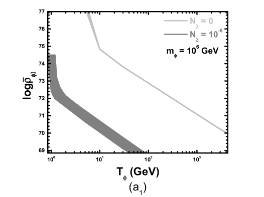
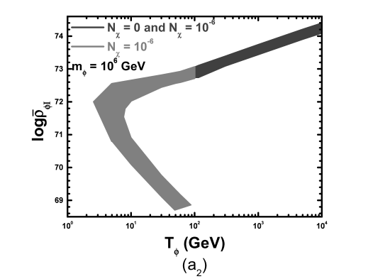
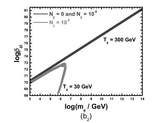
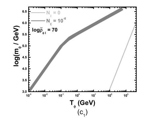
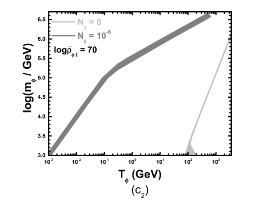
Figure 6: Regions allowed by eq. (2) on the $T_{\phi}-\log{\mbox{$\bar{\rho}_{\phi_{\rm I}}$}}$ plane ${\sf(a_{1},~{}a_{2})}$ for $m_{\phi}=10^{6}~{}{\rm GeV}$, $\log m_{\phi}-\log{\mbox{$\bar{\rho}_{\phi_{\rm I}}$}}$ plane ${\sf(b_{1},~{}b_{2})}$ for $T_{\phi}=30~{}{\rm GeV}$ and $T_{\phi}=300~{}{\rm GeV}$, and $T_{\phi}-\log m_{\phi}$ plane ${\sf(c_{1},~{}c_{2})}$ for $\log{\mbox{$\bar{\rho}_{\phi_{\rm I}}$}}=70$. We take $N_{\tilde{\chi}}=0$ or $N_{\tilde{\chi}}=10^{-6}$, $m_{\tilde{\chi}}=350~{}{\rm GeV}$ and $\langle\sigma v\rangle=10^{-10}~{}{\rm GeV^{-2}}~{}[\langle\sigma v\rangle=10^{-8}~{}{\rm GeV^{-2}}]~{}{\sf(a_{1},b_{1},c_{1}~{}[a_{2},b_{2},c_{2}])}$.

the upper left bounds of the allowed regions (possible further reduction of $T_{\phi}$ reduces also $\Omega_{\chi}h^{2}$ which turns out to be $\bar{\rho}_{\phi}$ independent, any more). In the dark grey [grey] allowed regions of fig. 6-${\sf(a_{2})}$, we obtain $q$-TD with EP [non-EPI] while $T_{\rm PL}$ ranges between (18 and 400) GeV [(1 and 15) GeV]. Due to the increase of the released entropy which is caused by the increase of $\bar{\rho}_{\phi_{\rm I}}$, $\Omega_{\chi}h^{2}$ decreases as $\rho_{\phi_{\rm I}}$ increases and so, the upper [lower] boundary of the dark grey and the almost horizontal part of the grey allowed region come from eq. (2a) [eq. (2b)] (note that eq. (54) is not applicable in this part of the grey allowed region). On the contrary, eq. (54) can be applied for the almost vertical part of the grey allowed region and so, its left [right] boundary comes from eq. (2a) [eq. (2b)]. The lower right limit of this region is found from eq. (22a) whereas the upper one is just conventional.

$\bullet$ $\log m_{\phi}-\log{\mbox{$\bar{\rho}_{\phi_{\rm I}}$}}$ plane for $T_{\phi}=30~{}{\rm GeV}$ and $T_{\phi}=300~{}{\rm GeV}$, in fig. 6-${\sf(b_{1})}$ and ${\sf(b_{2})}$. In the allowed areas we obtain $q$-TD. In the dark and light grey areas of fig. 6-${\sf(b_{1})}$ [fig. 6-${\sf(b_{2})}$] we have non-EPII [EP]. The dark grey regions are $N_{\chi}$-independent since the first term in the r.h.s of eq. (56a) [eq. (53)] dominates over the second one for non-EPII [EP]. In fig. 6-${\sf(b_{1})}$ the upper [lower] boundary of the allowed regions comes from eq. (2b) [eq. (2a)], whereas in fig. 6-${\sf(b_{2})}$, the origin of the boundaries is the inverse. This is because higher $\bar{\rho}_{\phi_{\rm I}}$’s result to hither $T_{\rm PL}$’s and so, $T_{\rm RD}$’s. This has as a consequence that the non-relativistic reduction of $f^{\rm eq}_{\chi}$ turns out to be less efficient, thereby increasing $\Omega_{\chi}h^{2}$ for non-EPII. For EP, the same effect causes mainly an increase to the released entropy and so, a reduction to $\Omega_{\chi}h^{2}$. Note, also, that since $c_{{}_{q\phi}}{\mbox{$\rho_{\phi_{\rm I}}$}}$ remains constant along the boundaries of the dark grey areas $T_{\rm PL}$ remains also constant – see eq. (41) – and is equal to $16~{}{\rm GeV}$ [$18~{}{\rm GeV}$] in fig. 6-${\sf(b_{1})}$ for $T_{\phi}=30~{}{\rm GeV}$ [$T_{\phi}=300~{}{\rm GeV}$] and $(32-38)~{}{\rm GeV}$ in fig. 6-${\sf(b_{2})}$. The upper [lower] limits of the dark grey or grey areas (in the upper right [lower left] corners) of these figures correspond to the upper [lower] bound of eq. (25). In the grey areas of fig. 6-${\sf(b_{1})}$ and ${\sf(b_{2})}$, we obtain non-EPI. Eq. (54) is applicable in the almost vertical parts of these areas and so, the left [right] boundary of the allowed regions comes from eq. (2b) [eq. (2a)] ($T_{\rm PL}$ ranges between (3 and 17-18) GeV). Eq. (54) is not applicable in the left upper branch of the area in fig. 6-${\sf(b_{2})}$ where the origin of the boundaries is the inverse ($T_{\rm PL}=(1-7)~{}{\rm GeV}$). The lower bound of the almost vertical part of these areas come from eq. (22a). Note, finally, that for $T_{\phi}=30~{}{\rm GeV}$ and $\langle\sigma v\rangle=10^{-8}~{}{\rm GeV^{-2}}$ – fig. 6-${\sf(b_{2})}$ – we are not able to construct allowed area for $N_{\chi}=0$. This is because $T_{\rm PL}\ll m_{\chi}/20$ and possible increase of $\bar{\rho}_{\phi_{\rm I}}$ (which could increase $T_{\rm PL}$) leads to $\Omega_{\chi}h^{2}$ close to $\Omega_{\chi}h^{2}|_{{\mbox{$\bar{\rho}_{\phi}$}}=0}$ which is lower than 0.09 due to large $\langle\sigma v\rangle$. However for $N_{\chi}=10^{-6}$, $\Omega_{\chi}h^{2}$ increases to an acceptable level.

$\bullet$ $T_{\phi}-\log m_{\phi}$ plane for $\log{\mbox{$\bar{\rho}_{\phi_{\rm I}}$}}=70$, in fig. 6-${\sf(c_{1})}$ and ${\sf(c_{2})}$. In the allowed regions of these figures, we obtain $q$-TD, besides the part of the grey area for $\log(m_{\phi}/{\rm GeV})<5.35$ where we get $q$-PD. For $N_{\chi}\neq 0$ we have non-EPI, whereas for $N_{\chi}=0$, we take non-EPII, except for the lower part of the light grey area (for $\log(m_{\phi}/{\rm GeV})<3.3$) where the EP is activated. As induced from eq. (54) [eq. (56)] for non-EPI [non-EPII], $f_{\chi}$ decreases as $m_{\phi}$ (and so, $\rho_{q_{\rm I}}$) decreases. Therefore, the upper [lower] boundary of the allowed regions comes from eq. (2a) [eq. (2b)]. The upper bound on the right corners of the allowed regions is derived from eq. (22a). The lower limits of the light grey areas and these of the lower left corner of the grey areas are extracted from the lower bound of eq. (25a). In the grey [light grey] areas $T_{\rm PL}$ ranges between (0.1 and 5) GeV [(16 and 20) GeV].

5 CONCLUSIONS

We studied the decoupling of a CDM candidate, $\chi$, in the context of a novel cosmological scenario termed KRS (“KD Reheating”). According to this, a scalar field $\phi$ decays, reheating the universe, under the total or partial domination of the kinetic energy density of another scalar field, $q$, which rolls down its exponential potential, ensuring an early KD epoch and acting as quintessence today. We solved the problem (i) numerically, integrating the relevant system of the differential equations (ii) semi-analytically, producing approximate relations for the cosmological evolution before and after the onset of the RD era and solving the properly re-formulated Boltzmann equation which governs the evolution of the $\chi$-number density. Although we did not succeed to achieve general analytical solutions in all cases, we consider as a significant development the derivation of a result for our problem by solving numerically just one equation, instead of the whole system above.

The model parameters were confined so as $H_{\rm I}=m_{\phi}$ and $\Omega^{\rm I}_{q}=1$. The current observational data originating from nucleosynthesis, acceleration of the universe and the DE density parameter were also taken into account. We considered two cases depending whether $\phi$ decays before ($q$-TD) or after ($q$-PD) it becomes the dominant component of the universe. We showed that, in both cases, the temperature remains frozen for a period at a plateau value $T_{\rm PL}$, which turns out to be much lower than its maximal value achieved during a pure reheating with the same initial $\phi$-energy density.

As regards the $\Omega_{\chi}h^{2}$ computation, we discriminated two basic types of $\chi$-production depending whether $\chi$’s do or do not reach chemical equilibrium with plasma. In the latter case, two subcases were singled out: the type I and type II non-EP. The type I non-EP is activated for $T_{\rm PL}\ll m_{\chi}/20$ and $N_{\chi}\neq 0$ is required so as sizable $\Omega_{\chi}h^{2}$ is achieved. The type II non-EP is activated for $T_{\rm PL}\sim m_{\chi}/20$. Finally, EP is applicable for $T_{\rm PL}\gg m_{\chi}/20$.

Next, we investigated the dependence of $\Omega_{\chi}h^{2}$ on the $\Omega_{q}({\mbox{$\leavevmode\hbox{\normalsize$\tau$\kern-5.0pt$\iota$}_{{}_{\rm NS}}$}})$ variations, generated by varying the free parameters $({\mbox{$\bar{\rho}_{\phi_{\rm I}}$}},~{}m_{\phi},~{}T_{\phi})$. We showed that mostly $\Omega_{\chi}h^{2}$ increases with $\Omega_{q}({\mbox{$\leavevmode\hbox{\normalsize$\tau$\kern-5.0pt$\iota$}_{{}_{\rm NS}}$}})$ when $T_{\rm PL}$ increases and it decreases as $\Omega_{q}({\mbox{$\leavevmode\hbox{\normalsize$\tau$\kern-5.0pt$\iota$}_{{}_{\rm NS}}$}})$ increases when $T_{\rm PL}$ decreases, too. Also, $\Omega_{\chi}h^{2}$ decreases as $\langle\sigma v\rangle$ increases for EP and non-EPI for large $\langle\sigma v\rangle$’s, it decreases with $\langle\sigma v\rangle$ for non-EPII and large $\langle\sigma v\rangle$’s and it remains constant for non-EPI and non-EPII for low $\langle\sigma v\rangle$’s. Finally, in any case, $\Omega_{\chi}h^{2}$ increases with $N_{\chi}$ and $m_{\chi}$.

Comparing the results on $\Omega_{\chi}h^{2}$ with those in the QKS and the LRS, we concluded that in the present scenario, $\Omega_{\chi}h^{2}$ does not exclusively increases with $\Omega_{q}({\mbox{$\leavevmode\hbox{\normalsize$\tau$\kern-5.0pt$\iota$}_{{}_{\rm NS}}$}})$ (in contrast with the QKS) and it approaches its value in the LRS as $\Omega_{q}({\mbox{$\leavevmode\hbox{\normalsize$\tau$\kern-5.0pt$\iota$}_{{}_{\rm NS}}$}})$ decreases. Finally, regions consistent with the present CDM bounds were constructed, using $m_{\chi}$’s and $\langle\sigma v\rangle$’s commonly allowed in several particle models. In most cases, the required $T_{\rm PL}$ is lower than about 40 GeV. As a consequence, simple, elegant and restrictive particle models such as the CMSSM [10] – which, due to the large predicted $\Omega_{\chi}h^{2}$, is tightly constrained in the SC [11] or almost excluded in the QKS [19, 34, 15] – can become perfectly viable in the KRS.