Finite size effects on pion spectra in relativistic heavy-ion collisions

Abstract

We compute the pion inclusive transverse momentum distribution assuming thermal equilibrium together with transverse flow and accounting for finite size effects and energy loss at the time of decoupling. We compare to data on mid-rapidity pions produced in central collisions in RHIC at $\sqrt{s_{NN}}=200$ GeV. We find that a finite size for the system of emitting particles results in a power-like fall-off of the spectra that follows the data up to larger $p_{t}$ values, as compared to a simple thermal model.

I Introduction

In recent years, strong evidence has been found in favor of the production of matter composed of the fundamental QCD degrees of freedom in central Au+Au collisions at the relativistic heavy-ion collider (RHIC) Bellwied ; STAR . Some of the quantitative understanding about the signals supporting these findings are associated to intermediate or high $p_{t}$ phenomena in particle spectra. Among these, the depletion in the production of large $p_{t}$ charged hadrons and neutral pions, as compared to extrapolations of data on p+p collisions to RHIC energies quenching , suggests that the fragmenting partons that give rise to final hadrons, loose energy on their way through the dense partonic matter believed to be formed during the early stages of the reaction. This phenomenon has been named jet quenching Gyulassy and has received stronger experimental support from the results of the d+Au mode at RHIC dAu . Moreover, the behavior of the proton to pion ratio for intermediate $p_{t}\sim 2$ GeV PHENIXBM suggests that an important mechanism of hadron production at RHIC is the thermal recombination of free quarks recomb during the evolution of the collision.

In spite of the success of this conceptual framework to interpret RHIC data, there is an ingredient commonly overlooked: the fact that all these phenomena take place during small time scales and consequently within small volumes.

Although not commonly considered, it is certainly true that small size effects are important in the description of statistical systems. For example, finite size effects have influence on the late-stage growth of nucleated bubbles during a first order phase transition Raju . Also, in the statistical hadronization model, the states used for the description are in general different to the observed asymptotic ones but such difference is not an issue unless the volume of the system is small, typically of order ${\mathcal{O}}(10\ {\mbox{f}m})^{3}$ Becattini . Finite size effects are also known to influence the interpretation of the correlation lengths in Hanbury Brown-Twiss analysis in the context of relativistic heavy-ion collisions Zhang ; Ayalaint .

Finite size effects on particle spectra have also been recently investigated Mostafa ; Ayalanoex ; Ayalaex , where these were referred to as boundary effects. The scenario considered in the last two of these studies resorts to a mean field treatment of the interactions affecting the most abundantly produced particles in the reactions, namely pions. It was argued that prior to kinetic freeze-out, the pion mean free path is smaller than the pion interaction range and therefore that during this stage, pions are still strongly interacting, mainly attractively, among themselves. The system resembles more a liquid than a gas, with a surface tension acting as a reflecting boundary. When assuming thermalization at freeze-out, the pion spectrum can be computed from the sum of the square of the wave function in momentum space weighed by the thermal occupation number for each state.

Qualitatively, the behavior of particle spectra including this finite size effects deviates from a simple exponential fall-off at high momentum since from the Heisenberg uncertainty principle, the more localized the states are in coordinate space, the wider their spread will be in momentum space. In terms of the discrete set of energy states describing the pion system, this behavior can be understood as arising from a higher density of states at large energy as compared to a calculation without boundary.

In this work we compute the transverse momentum distribution for pions assuming thermal equilibrium together with transverse flow and accounting for finite size effects at decoupling. By comparing to data on pion spectra on Au+Au collisions at $\sqrt{s_{NN}}=200$ GeV PHENIXBM ; PHENIX2 , we show that for temperatures and collective transverse flow within the commonly accepted values, the transverse momentum distributions can be described up to larger values of $p_{t}$ as compared to a simple exponential fall-off.

The paper is organized as follows: In Sec. II, we present the basics of the model to compute the pion spectra including finite size effects. In Sec. III, we compute the thermal pion spectrum including the effects of transverse flow together with the description of finite size effects. We carry out a systematic study of the behavior of the spectra when varying the parameters involved. In Sec. IV we compare the calculation to data on pion transverse distributions from Au+Au collisions at $\sqrt{s_{NN}}=200$ GeV and show how this model pushes the thermal component of the spectrum to larger $p_{t}$ values as compared to a simple exponential description. Finally we summarize and conclude in Sec. V.

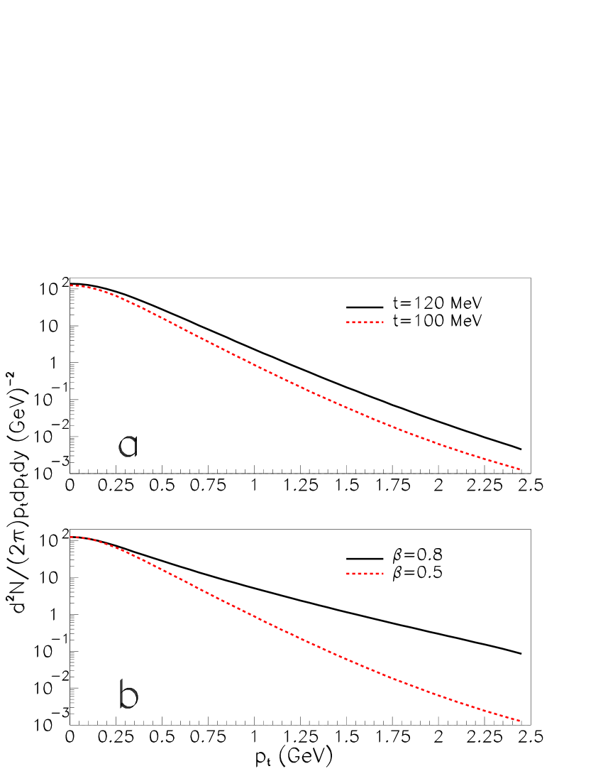
Figure 1: Invariant pion distribution as a function of $p_{t}$ for different combinations of the parameters $T$ and $\beta$ for a fixed value $R=8$ fm. The normalization is arbitrary.

II The model

When the system of particles can be considered as confined and their wave functions as satisfying a given condition at the boundary just before freeze out, the energy states form a discrete set. The shape of the volume within the confining boundary is certainly an important issue in case the model aims to describe transverse momentum particle distribution at all rapidities. However, in this work we will restrict ourselves to describe spectra at central rapidities. We thus consider a scenario in which the system of particles of a given species is in thermal equilibrium and is confined within a sphere of radius $R$ (fireball) as viewed from the center of mass of the colliding nuclei at the time of decoupling. This time needs not be the same over the entire reaction volume. Nevertheless, in the spirit of the fireball model we consider that decoupling takes place over a constant time surface in space-time. This assumption should be essentially correct if the freeze-out interval is short compared to the system’s life time.

The solutions that incorporate the effects of a finite size system have been found in Ref. Ayalanoex . They are given as the stationary solutions to the equation

$$\left(\frac{\partial^{2}}{\partial t^{2}}-\nabla^{2}+m^{2}\right)\psi({\mathbf{r}},t)=0$$ (1)

subject to the condition

$$\psi(|{\mathbf{r}}|=R,t)=0\,,$$ (2)

and also finite at the origin. The normalized stationary states are

$$\psi_{nlm^{\prime}}({\mathbf{r}},t) = \frac{1}{R\ J_{l+3/2}(k_{nl}R)}\left(\frac{1}{rE_{nl}}\right)^{1/2}$$ (3)

$$Y_{lm^{\prime}}(\hat{r})J_{l+1/2}(k_{nl}r)e^{-iE_{nl}t}$$

where $J_{\nu}$ is a Bessel function of the first kind and $Y_{lm^{\prime}}$ is a spherical harmonic. The parameters $k_{nl}$ are related to the energy eigenvalues $E_{nl}$ by

$$E_{nl}^{2}=k_{nl}^{2}+m^{2}$$ (4)

and are given as the solutions to

$$J_{l+1/2}(k_{nl}R)=0\,.$$ (5)

Figure 2: Pion rapidity distribution for $T=120$ MeV, $\beta=0.6$ and $R=8$ fm. The normalization is arbitrary.

Thus, the eigenfunctions for the bound system of particles are given explicitly by Eq. (3). These are analytical, albeit given in terms of Bessel functions.

III Thermal spectrum

The contribution to the thermal particle invariant distribution from a state with quantum numbers $\{n,l,m^{\prime}\}$ is given by

$$E\frac{d^{3}N_{nlm^{\prime}}}{d^{3}p}=\int\frac{d\sigma}{(2\pi)^{3}}(k_{nl}\cdot u)f(k_{nl}\cdot v){\mathcal{W}}_{nlm^{\prime}}({\mathbf{p}},{\mathbf{r}}),$$ (6)

where ${\mathcal{W}}_{nlm^{\prime}}({\mathbf{p}},{\mathbf{r}})$ is the Wigner transform and $f(k_{nl}\cdot v)$ the thermal occupation factor of the state $\psi_{nlm^{\prime}}$, respectively. The four-vectors $v^{\mu}$ and $u^{\mu}$ represent the collective flow four-velocity and a four-vector of magnitude one, normal to the freeze-out hypersurface $\sigma$, respectively.

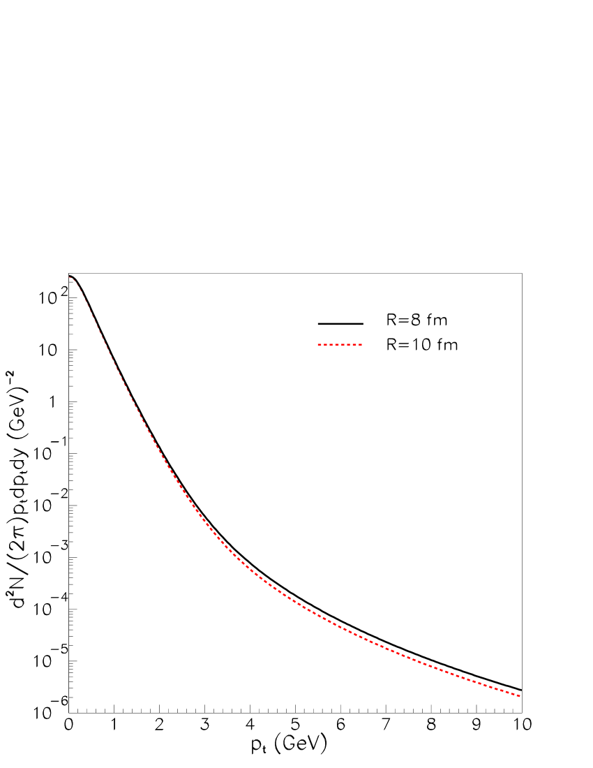
Figure 3: Invariant pion distribution as a function of $p_{t}$ for two values of the parameter $R$ and fixed values $T=120$ MeV and $\beta=0.6$. The normalization is arbitrary.

For the system of bound bosons, the Wigner transform of a given state is defined as

$${\mathcal{W}}_{nlm^{\prime}}({\mathbf{p}},{\mathbf{r}}) = \int d^{3}r^{\prime}e^{-i{\mathbf{p}}\cdot{\mathbf{r}}}$$ (7)

$$\psi^{*}_{nlm^{\prime}}({\mathbf{r}}+\frac{\mathbf{r^{\prime}}}{2},t)\frac{\stackrel{{\scriptstyle\leftrightarrow}}{{\partial}}}{\partial t}\psi_{nlm^{\prime}}({\mathbf{r}}-\frac{\mathbf{r^{\prime}}}{2},t).$$

In order to consider a situation where freeze-out happens at a fixed time and within a spherical volume of radius $R$, the unit four-vector $u^{\mu}$ can be chosen as $u^{\mu}=(1,{\mathbf{0}})$.

To keep matters simple, we consider a thermal occupation factor of the Maxwell-Boltzmann kind, namely

$$f(k_{nl}\cdot v)=e^{-k_{nl}\cdot v/T},$$ (8)

where $T$ is the system’s temperature. The four-vector $v^{\mu}$ is parametrized as

$$v^{\mu}=\gamma(1,{\mathbf{v}}),$$ (9)

and we choose a radial profile for the vector ${\mathbf{v}}$ such as

$${\mathbf{v}}=\beta\frac{\mathbf{r}}{R},$$ (10)

where the parameter $\beta$ represents the surface expansion velocity. Notice that, the radial profile for the expansion velocity considered in Eq. (10) can be taken as the transverse component of the flow only for the description of central rapidity data. Correspondingly, the gamma factor is given by

$$\gamma=\frac{1}{\sqrt{1-\left(\beta\frac{r}{R}\right)^{2}}}.$$ (11)

Nonetheless, in order to continue to keep matters as simple as possible, and be able to analytically perform the integrations in Eq. (6), we will instead consider that the gamma factor is a constant evaluated at the average transverse expansion velocity, namely,

$$\gamma\rightarrow\bar{\gamma}=\frac{1}{\sqrt{1-(3\beta/4)^{2}}}.$$ (12)

We take the four-vector $k_{nl}^{\mu}$ given by

$$k_{nl}^{\mu}=(E_{nl},{\mathbf{k}}_{nl}),$$ (13)

and choose ${\mathbf{k}}_{nl}\parallel{\mathbf{p}}$. This choice is motivated from the continuum, boundless limit, where the relativistically invariant exponent in the thermal occupation factor becomes $\gamma(E-{\mathbf{p}}\cdot{\mathbf{v}})$.

Figure 4: Nuclear suppression factor $R_{AA}$ for neutral pions from Ref. PHENIX2 parametrized in the interval from 1 to 10 GeV. The parametrization is chosen as to become a constant for large $p_{t}$ values.

Gathering the elements described in Eqs. (7) to (13), it is straightforward to evaluate the integral in Eq. (6). Summing over all the states, the invariant thermal distribution is given by

$$E\frac{d^{3}N}{d^{3}p} = {\mathcal{N}}\sum_{nl}\frac{(2l+1)}{(2\pi)}\frac{k_{nl}^{2}E_{nl}\ e^{-\bar{\gamma}E_{nl}/T}}{\sqrt{p^{2}+\left(\frac{\bar{\gamma}\beta k_{nl}}{2RT}\right)^{2}}}$$ (14)

$$\times \frac{\left|J_{l+1/2}\left(pR-i\frac{\bar{\gamma}\beta k_{nl}}{2T}\right)\right|^{2}}{\left[p^{2}-k_{nl}^{2}-\left(\frac{\bar{\gamma}\beta k_{nl}}{2RT}\right)^{2}\right]^{2}+\left[\frac{\bar{\gamma}\beta pk_{nl}}{RT}\right]^{2}},$$

where the factor $(2l+1)$ comes from the degeneracy of a state with a given angular momentum eigenvalue $l$ and ${\mathcal{N}}$ is a normalization constant.

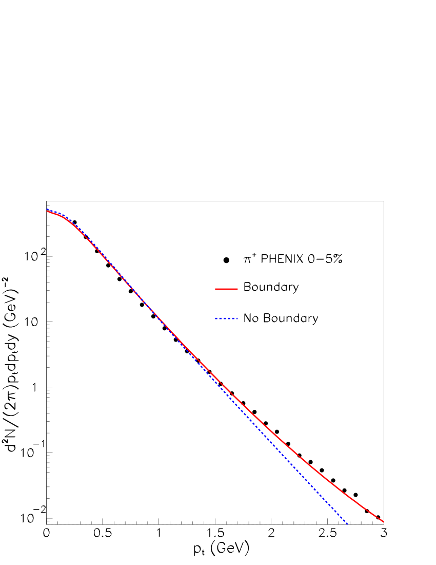
Figure 5: Invariant pion distribution as a function of $p_{t}$ for $R=8$ fm, $T=120$ MeV and $\beta=0.6$ compared to data on mid rapidity positive pions from central collisions at $\sqrt{s_{NN}}=200$ GeV measured by PHENIX. The normalization of the model theoretical curve has been fixed from a fit to the data.

Figure 1 shows the invariant pion distribution as a function of $p_{t}$ for different combinations of the parameters $T$ and $\beta$ and a fixed value $R=8$ fm. Figure 1$a$ shows the distribution for two different temperatures $T=100,\ 120$ MeV and $\beta=0.5$. As expected, the effect of increasing the temperature is to increase the inverse slope of the distribution. Figure 1$b$ shows the distribution for two different values of the surface expansion velocity, $\beta=0.5,\ 0.8$ and $T=100$ MeV. The effect of increasing the expansion velocity is also to increase the inverse slope of the distribution. Figure 2 shows an example of the kind of rapidity distributions obtained in the model. Notice that the distribution is not as broad as data seem to indicate (see for example Ref. BRAHMS .) This is a limitation of the spherical symmetry assumed in the model emphasizing the need of restricting its applicability to the description of central rapidity data.

Figure 3 shows the distribution for two different values of the confining radius $R=8,\ 10$ fm for fixed values of $T=120$ MeV and $\beta=0.6$. The effect of increasing the confining radius is to increase the value of $p_{t}$ for which the distribution has a point of inflexion towards a concave shape. This is to be expected since in the limit where the confining volume goes to infinity, the value of $p_{t}$ for this point of inflexion should also go to infinity as the system becomes boundless.

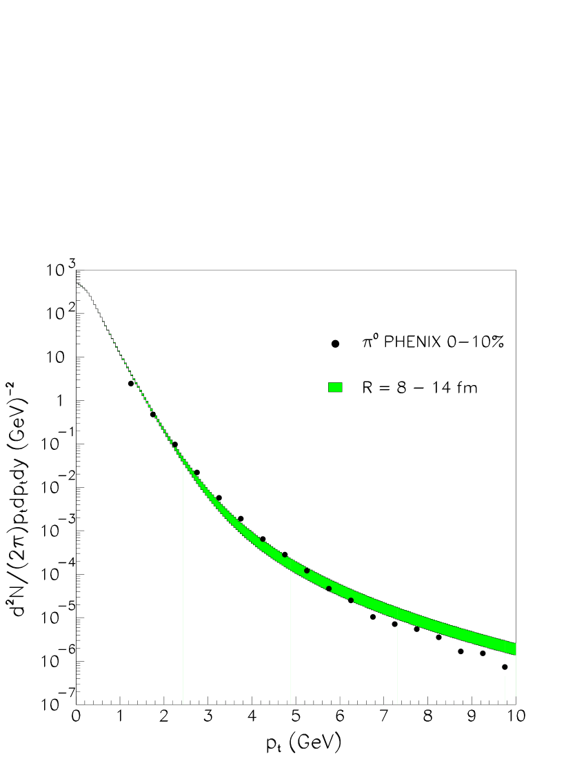
Figure 6: Invariant pion distribution as a function of $p_{t}$ for $T=120$ MeV, $\beta=0.6$ for values of $R=8$ fm (upper curve) to $R=14$ fm (lower curve), compared to data on mid rapidity neutral pions from central collisions at $\sqrt{s_{NN}}=200$ GeV measured by PHENIX. The normalization of the curves has been taken from the fit to the $\pi^{+}$ spectrum.

IV Pion spectra

In order to test the model, we compare the theoretical distribution to data on mid-rapidity pions produced in RHIC central collisions at $\sqrt{s_{NN}}=200$ GeV PHENIXBM ; PHENIX2 . Rather than performing an overall fit to find the optimum parameters, we fix them to values within the commonly accepted ones to describe freeze-out conditions.

To include the effects of parton energy loss, we resort to parametrize the data on $R_{AA}$ for neutral pions as measured by PHENIX PHENIX2 . We use the the expression

$$\frac{A}{e^{x-B}+1}+C\,,$$ (15)

and find from a fit to the data on $R_{AA}$ the values $A=0.18$, $B=3.17$ and $C=0.20$. This parametrization is taken in such a way that for large $p_{t}$ the nuclear suppression factor remains a constant. This is shown in Fig. 4.

First we describe data for the low $p_{t}$ part of the spectra. This is done in Fig. 5 where we show the invariant pion distribution as a function of $p_{t}$ for $R=8$ fm, $T=120$ MeV and $\beta=0.6$, including the energy loss effect, compared to data on $\pi^{+}$ from PHENIX PHENIXBM . The normalization of the model theoretical curve has been calculated from a fit to the data. We notice from Fig. 5 that the curve does a very good job describing the data for all values of $p_{t}$. In contrast, a calculation where no effects of a finite size are included, and thus the wave function of a given state is simply a plane wave, does not describe the data over the considered range when we use the same values for $T$ and $\beta$ as for the case of the calculation with a confining volume. This is also shown in Fig. 5 where we notice the more steep fall-off of the curve without finite size effects.

Next we describe data in the range 1 GeV $<p_{t}<$ 10 GeV. This is done in Fig. 6 where we show the invariant pion distribution as a function of $p_{t}$ for $T=120$ MeV, $\beta=0.6$ and $R=8-14$ fm, including the energy loss effect, compared to data on neutral pions from PHENIX PHENIX2 . The normalization of the curves has been taken from the fit to the $\pi^{+}$ spectrum. The model does a good description of data for values of the parameter $R$ between 8 and 10 fm up to $p_{t}\sim 3$ GeV from where the curves start deviating from the data that shows a steeper fall-off. This failure is however expected since for large $p_{t}$ the leading particle production mechanism is the fragmentation of fast moving partons, some of which fragment outside the fireball region and thus are not influenced by the confining boundary that the rest of the particles experience within the fireball.

V Summary and conclusions

In this work we have computed the pion transverse momentum distribution in a thermal model including transverse expansion and accounting for the fact that the system of particles is produced within a small volume up to freeze-out, in the context of relativistic heavy-ion collisions. The finite size has been introduced by requiring that the system’s wave functions vanish at the boundary but remain finite at the origin. The net effect is a broadening of the particle transverse momentum distribution with respect to a simple thermal model without a boundary. The physical origin of this broadening is the Heisenberg uncertainty principle since as the states are more localized in coordinate space, their spread is wider in momentum space. Energy loss has also been considered by a parametrization of the experimentally measured nuclear suppression factor $R_{AA}$ where we require that this becomes constant for large $p_{t}$ values.

The model does a very good job describing data for low to intermediate $p_{t}$ in the range $0<p_{t}\lesssim 3$ GeV for commonly accepted values of the temperature $T=120$ MeV and the surface transverse expansion velocity $\beta=0.6$ (corresponding to an average transverse expansion velocity $\langle\beta\rangle\simeq 0.5$) when the system’s radius $R$ at freeze-out is in the range 8 fm $\lesssim R\lesssim$ 10 fm. This is best seen when comparing the model to data on charged pions produced in central Au + Au collisions. The description of data for $p_{t}$ in the range $3\lesssim p_{t}<10$ is not as good as can be seen from a comparison of the model to the spectrum of neutral pions produced in central Au + Au collisions. This behavior is not surprising though, since for large $p_{t}$ it is well known that the leading particle production mechanism is the fragmentation of fast moving partons, some of which fragment outside the fireball region and thus are not influenced by the confining boundary, or mean field, that the rest of the particles experience within the fireball.

We thus conclude that the thermal features of the spectrum, which are obtained from the low $p_{t}$ region, are best highlighted when accounting for the finite size of the system at decoupling. It is of course interesting to check the consistency of this treatment when extended to the case of fermions, and in particular protons. Finally, it is worth to note that finite size effects should also play a role during the partonic phase of the collision Wong and in particular that they can also influence the recombination scenario. This kind of analyses is for the future.

References

- (1) R. Bellwied, Nucl. Phys. A 752, 398c (2005).
- (2) J. Adams et al. (STAR Collaboration), Nucl. Phys. A 757, 102 (2005).
- (3) K. Adcox et al. (PHENIX Collaboration), Phys. Rev. Lett. 88, 022301 (2002); C. Adler et al. (STAR Collaboration), dPhys. Rev. Lett. 89, 202301 (2002); B.B. Back et al. (PHOBOS Collaboration), Phys. Lett. B 578, 297 (2004).
- (4) M. Gyulassy and M. Plumer, Phys. Lett. B 243, 432 (1990); X.N. Wang and M. Gyulassy, Phys. Rev. Lett. 68, 1480 (1992).
- (5) K. Adcox et al. (PHENIX Collaboration), Phys. Rev. Lett. 91, 072303 (2003); C. Adler et al. (STAR Collaboration), Phys. Rev. Lett. 91, 072304 (2003); B.B. Back et al. (PHOBOS Collaboration), Phys. Rev. Lett. 91, 072302 (2003).
- (6) S.S. Adler et al. (PHENIX Collaboration), Phys. Rev. C 69, 034909 (2004).
- (7) R. C. Hwa and C. B. Yang, Phys. Rev. C 67, 034902 (2003); R. J. Fries, B. Müller, C. Nonaka, and S. A. Bass, Phys. Rev. Lett. 90, 202303 (2003); V. Greco, C. M. Ko, and P. Lévai, Phys. Rev. Lett. 90, 202302 (2003).
- (8) E.S. Fraga and R. Venugopalan, Braz. J. Phys. 34, 315 (2004); Physica A345, 121 (2004).
- (9) F. Becattini, J. Phys. Conf. Ser. 5, 175 (2005).
- (10) Q.H. Zhang and S.S. Padula, Phys. Rev. C 62, 024902 (2000); Q.H. Zhang, “Constraints on the size of the quark-gluon plasma”, hep-ph/0106242.
- (11) A. Ayala and A. Sánchez, Phys. Rev. C 63, 064901 (2001).
- (12) M. Mostafa and C.Y. Wong, Phys. Rev. C 51, 2135 (1995).
- (13) A. Ayala and A. Smerzi, Phys. Lett. B 405, 20 (1997).
- (14) A. Ayala, J. Barreiro and L.M. Montaño, Phys. Rev. C 60, 014904 (1999).
- (15) S.S. Adler, et al., PHENIX Collaboration, Phys. Rev. Lett. 91, 072301 (2003).
- (16) I.G. Bearden, et al., BRAHMS Collaboration, Phys. Rev. Lett. 94, 162301 (2005).
- (17) C.-Y. Wong, Phys. Rev. C 48, 902 (1993).