Gauge-Higgs unification with brane kinetic terms

Abstract

By identifying the Higgs field as an internal component of a higher dimensional gauge field it is possible to solve the little hierarchy problem. The construction of a realistic model that incorporates such a gauge-Higgs unification is an important problem that demands attention. In fact, several attempts in this direction have already been put forward. In this letter we single out one such attempt, a 6D SU(3) extended electroweak theory, where it is possible to obtain a Higgs mass prediction in accord with global fits. One shortcoming of the model is its prediction for the Weinberg angle, it is too large. We slightly modify the model by including brane kinetic terms in a way motivated by the orbifold action on the 6D fields. We show that in this way it is possible to obtain the correct Weinberg angle while keeping the desired results in the Higgs sector.

1 Introduction

The little hierarchy problem consists on the following: treating the standard model as a low-energy effective theory valid up to a scale $\Lambda$, the Higgs mass suggested by global fits of electroweak precision data is natural for $\Lambda\sim 500$ GeV. However, there are bounds at present coming from four fermion operators that demand $\Lambda\sim 10$ TeV. Thus there is an order of magnitude discrepancy.

A good amount of work has recently been devoted to find a solution to this problem. As it is well known, supersymmetry is at the moment the best candidate for the solution of the hierarchy problem. In this context, the discrepancy in scales is translated to a discrepancy between the Higgs mass $m_{h}$ and the scale of sparticle masses $m_{SUSY}$. Depending on the specific model, MSSM, NMSSM, etc., there are several proposals that attempt to solve or ameliorate the little hierarchy problem [1, 2, 3, 4]. Other interesting scenario is that of Little Higgs models with and without T-Parity [5, 6, 7], where the Higgs boson is identified as a pseudo-goldstone boson of some unspecified strongly interacting sector.

A different line of work is that of theories in extra dimensions where the Higgs boson is an internal component of a gauge field of some extended electroweak symmetry. This idea is not new [8, 9] and recently has attracted attention as an alternative [10, 11, 12, 13, 14, 15]. In particular, Scrucca, Serone, Silvestrini and Wulzer [16] presented a complete analysis of an SU(3) electroweak gauge theory in six dimensions where the two extra dimensions have the geometry $T^{2}/{\mathcal{Z}}_{N}$. They find that it is possible to formulate a theory with just one Higgs doublet that gives the prediction (at leading order): $m_{H}=2m_{W}$. At its barest, their model gives a nice result with little effort. However, in order to get closer to a realistic theory there are a couple of issues that need to be addressed. One of them is the stability of the electroweak scale which has in fact been studied thoroughly for this model in [17], and more generally in [18] (see also [19]). The second issue is the fact that the prediction obtained for $\tan\theta_{W}$ is larger than the correct value.

In this letter we present a simple extension of the original framework where it is possible to obtain the correct value of the Weinberg angle while keeping similar results in the Higgs sector. The basic idea is to introduce brane kinetic terms for the components of the gauge field in a way motivated by the orbifold (geometrical) construction of the theory and see that their inclusion allows us to fix the problem. In Section 2 we review the basic results obtained in [16] and stress the problems mentioned above. Then, in Section 3 we present our extension based on the inclusion of brane kinetic terms in the theory. We present an example in detail and comment on other possibilities to then finish with our conclusions.

2 SU(3) in 6D

In this section we review the model presented in [16]. As mentioned in the Introduction, the basic idea is to relate the extra components of extra-dimensional gauge bosons to the 4D Higgs field.

Consider an SU(3) gauge theory in six dimensions, two of which are compactified on a $T^{2}/{\mathcal{Z}}_{N}$ orbifold ($T^{2}$ is the torus). Different choices of $N$ lead to different possibilities for the Higgs fields; for example for $N=3,4,6$ one can construct models with a single Higgs doublet [16]. In this letter we are interested in these models and will consider the case $N=3$.

Gauge bosons are denoted as $A_{\hat{\mu}}$, with the 6D index $\hat{\mu}=0,1,2,3,5,6$ split into $\mu=0,\ 1,\ 2,\ 3$ and $M=5,\ 6$. The full gauge symmetry is broken by the orbifold boundary conditions (O.B.C.) in such a way that the gauge symmetry can be broken as: $G\to H$, with $H={\rm SU(2)}_{W}\times{\rm U(1)}_{Y}$. Thus, O.B.C. split the group generators into two sets, $T^{A}=\{T^{a},T^{k}\}$, where $T^{A}\,\epsilon\,G$ and $T^{a}\,\epsilon\,H$. From this one obtains that $A^{a}_{\mu}$ and $A^{a}_{M}$ have zero modes in the spectrum whereas $A^{k}_{\mu}$ does not. Note that a vacuum expectation value for $A^{a}_{M}$ can break the symmetry further, namely from $H\to H^{\prime}=U(1)_{em}$

Then, in the SU(3) model that we are considering, the orbifold action on the gauge fields $A_{\hat{\mu}}$, is such that the invariant components become $W_{\mu}=A_{\mu}=\sum_{a}A_{\mu a}\frac{\lambda^{a}}{2}$ and $H_{M}=A_{M}=\sum_{a}A_{Mb}\frac{\lambda^{b}}{2}$, where $a=1,\ 2,\ 3$; $b=4,\ 5,\ 6,\ 7$ and $\lambda$ are the Gell-Mann matrices. Note that these expressions are valid for the 6D gauge fields and so after compactification we identify the usual 4D gauge bosons with the zero modes of the Kaluza-Klein tower. From now on we concentrate only on these zero modes and will omit any ($0$) superscript on the 4D fields.

The zero modes of the 4D vector fields above can be expressed in matrix notation as

$$A_{\mu} = \frac{1}{2}\left(\begin{array}[]{ccc}A_{\mu}^{(3)}+\frac{1}{\sqrt{3}}A_{\mu}^{(8)}&A_{\mu}^{(1)}-iA_{\mu}^{(2)}&0\\ A_{\mu}^{(1)}+iA_{\mu}^{(2)}&-A_{\mu}^{(3)}+\frac{1}{\sqrt{3}}A_{\mu}^{(8)}&0\\ 0&0&-\frac{2}{\sqrt{3}}A_{\mu}^{(8)}\end{array}\right)$$ (4)

$$= \frac{1}{2}\left(\begin{array}[]{ccc}W_{\mu}^{(3)}+\frac{1}{\sqrt{3}}B_{\mu}^{(8)}&\sqrt{2}W_{\mu}^{+}&0\\ \sqrt{2}W_{\mu}^{-}&-W_{\mu}^{(3)}+\frac{1}{\sqrt{3}}B_{\mu}^{(8)}&0\\ 0&0&-\frac{2}{\sqrt{3}}B_{\mu}^{(8)}\end{array}\right)\,,$$ (8)

where we have introduced the usual SU(2) notation. In turn the 4D scalar fields are identified as

$$H_{M} = \frac{1}{2}\left(\begin{array}[]{ccc}0&0&A_{M}^{(4)}+iA_{M}^{(5)}\\ 0&0&A_{M}^{(6)}+iA_{M}^{(7)}\\ A_{M}^{(4)}-iA_{M}^{(5)}&A_{M}^{(6)}-iA_{M}^{(7)}&0\end{array}\right)$$ (12)

$$= \frac{1}{\sqrt{2}}\left(\begin{array}[]{ccc}0&0&H^{*+}_{M}\\ 0&0&H^{0}_{M}\\ H^{-}_{M}&H^{0*}_{M}&0\end{array}\right)\,.$$ (16)

Substituting these expressions into the Lagrangian for the zero modes obtained after integration over the internal torus one gets

$${\cal L}_{4} = -\frac{1}{4}(F_{\mu\nu}^{a})^{2}-\frac{1}{4}(B_{\mu\nu})^{2}+\left|\left(\partial_{\mu}-ig_{4}W_{\mu}^{a}\frac{\tau^{a}}{2}-ig_{4}\sqrt{3}\frac{1}{2}B_{\mu}\right){\cal H}\right|^{2}$$ (17)

$$- \frac{g_{4}^{2}}{2}|{\cal H}|^{4}\,,$$

with $g_{4}=g_{6}/(\frac{2}{N}\pi\sqrt{R_{5}R_{6}})$ as the 4D gauge coupling and ${\cal H}^{T}=\left(\begin{array}[]{cc}H^{*+}_{M}&H^{0}_{M}\end{array}\right)$ the Higgs doublet. $R_{5,6}$ denote the radii of the torus.

One can immediately obtain some interesting Higgs physics results out of this simple model. Note that a Higgs tree-level potential is present : this is to be contrasted with the 5D case where this is not the case and one obtains Higgs masses that are very small [16]. In the present case, if one makes the (strong) assumption that local operators (tadpole operators) have no significant effect on the potential and ignoring logarithmic divergences, the leading one-loop effective potential for the Higgs is

$$V({\cal H})=-\mu^{2}|{\cal H}|^{2}+\lambda|{\cal H}|^{4}\,,$$ (18)

where $\mu^{2}$ is generated radiatively. By assuming that $\mu^{2}>0$ and setting $\langle|{\cal H}|\rangle=v/\sqrt{2}$ one obtains $m_{H}=\sqrt{2}\mu=\sqrt{2\lambda}v$ and $m_{W}=gv/2$. Taking the ratio leads to

$$\frac{m_{H}}{m_{W}}=\frac{2\sqrt{2\lambda}}{g_{4}}=2\,,$$ (19)

where we use the fact that $\lambda=g_{4}^{2}/2$.

It is interesting that this simple model leads to a Higgs mass in approximately the right range suggested by global fits. In order to make it more realistic however one needs to understand the details regarding the tadpole operators that give the main radiative corrections to the result. As mentioned in Section 1, the origin of these operators has been studied in [18] where they found that tadpoles are always allowed in orbifolds compactifications based on $T^{D-4}/{\mathcal{Z}}_{N}$ ($D$ even, $N>2$). Another interesting result is that on $T^{D-4}/{\mathcal{Z}}_{2}$ with arbitrary $D$, tadpoles can only appear in $D=6$ (except for models with only bulk gauge fields). In [16], an argument was presented that a globally vanishing one-loop tadpole is indeed harmless for the stability of electroweak symmetry breaking. Thus, constructing a model with globally vanishing tadpoles is a way to go and one can do this by introducing a suitable fermion content [17].

Another problem with the model is that it gives $\tan\theta_{W}=\sqrt{3}$, which is larger than the measured value. It is therefore interesting to see if one can find modifications of this model that would fix this problem and at the same time keep all the nice features in the Higgs sector. As suggested in [16], it might be possible to lower the value of $\tan\theta_{W}$ by adding extra U(1) symmetries, however there can be other possibilities. In this letter we present an alternative where the basic idea is to introduce brane kinetic terms in the 6D theory and explore their effects on the Higgs mass.

3 Brane kinetic terms

In this section we describe how the addition of localized brane kinetic terms can be used to lower the prediction for $\tan\theta_{W}$. A discussion on brane kinetic terms and their physical implications can be found in [21, 22, 23, 24]. As mentioned in the previous section, we are interested in models with one Higgs doublet an will present our analysis for an SU(3) theory compactified on $T^{2}/{\mathcal{Z}}_{3}$.

3.1 Brane kinetic terms at a point

We start with the following 6D Gauge Lagrangian:

$${\cal L}_{6D}=-\frac{1}{4}\left(\left(F_{\hat{\mu}\hat{\nu}}\right)^{2}+\delta(x_{5})\delta(x_{6})\left[c_{1}\left(F^{(a)}_{\mu\nu}\right)^{2}+c_{2}\left(F^{(8)}_{\mu\nu}\right)^{2}\right]\right)\,,$$ (20)

where again $a=1,2,3$. In eq. (20) we have added a localized kinetic term to the SU(3) 6D gauge theory at the fixed point $x_{5}=x_{6}=0$  and taken $c_{1}$ and $c_{2}$ as positive constants with mass dimension $-2$. Note that we have introduced two different strengths in the localization terms. This choice is certainly a source of fine tuning in the model and at this moment we do not have a precise argument for it but to say that it is motivated by the geometrical breaking of the symmetry, where the orbifold action is already differentiating the components of the gauge fields. We will see that this differentiation will play a crucial role in determining a correct value for $\tan\theta_{W}$. In this particular example and for simplicity, we have added brane kinetic terms only to those components of the 6D gauge fields that will become 4D gauge fields and not to the scalar ones.

After compactification the 4D Lagrangian for the zero modes becomes (in SU(2) notation)

$${\cal L}_{4D}^{(0)} = -\frac{1}{4}(F_{\mu\nu}^{a})^{2}-\frac{1}{4}(B_{\mu\nu})^{2}+\left|\left(\partial_{\mu}-i\frac{g_{4}}{\sqrt{{\cal Z}_{1}}}W_{\mu}^{a}\frac{\tau^{a}}{2}-i\frac{g_{4}}{\sqrt{{\cal Z}_{2}}}\sqrt{3}\frac{1}{2}B_{\mu}\right){\cal H}\right|^{2}$$ (21)

$$- \frac{g_{4}^{2}}{2}|{\cal H}|^{4}\,,$$

where

$${\cal Z}_{1,2}=1+\frac{c_{1,2}}{(2\pi/3)^{2}R_{5}R_{6}}\ .$$ (22)

These factors, ${\cal Z}_{1}$ and ${\cal Z}_{2}$, have been introduced in order to properly normalize the fields in the 4D effective theory.

As before, we obtain a tree-level quartic Higgs coupling. Note however that it is now possible to fix the correct value for $\tan\theta_{w}$ by a suitable choice of ${\cal Z}_{1,2}$. This is where the effect of having different strengths for the brane kinetic terms appears. In order to see this explicitly we define $g=g_{4}/\sqrt{{\cal Z}_{1}}$ and $g^{\prime}=\sqrt{3}g_{4}/\sqrt{{\cal Z}_{2}}$ as the SU(2)_W and U(1)_Y gauge couplings respectively. Then, using the same arguments that led to eq. (19), we obtain

$$\tan\theta_{W}=\frac{g^{\prime}}{g}=\sqrt{\frac{3{\cal Z}_{1}}{{\cal Z}_{2}}}\,$$ (23)

while the Higgs boson mass is now given by

$$\frac{m_{H}}{m_{W}}=2\sqrt{{\cal Z}_{1}}\ .$$ (24)

In order to explore some of the parameter space, we consider the particular case of a torus of dimensions $R\equiv R_{5}=R_{6}$. We then identify a compactification scale $M_{C}=1/R$ for each of the two extra dimensions.

Figure 1 shows the values of $c_{1}$ and $c_{2}$ consistent with the correct value of $\tan\theta_{W}$ for three choices of $M_{C}=1/R$: $10$, $30$ and $100$ TeV. We see that in all three cases, a solution requires $c_{2}>c_{1}$. Furthermore, solutions exist for $c_{2}\leq 1$. This is relevant since our analysis incorporates only the zero modes and thus is valid only for the case in which the both $c_{1}$ and $c_{2}$ are small. Larger values would require a systematic study of KK modes mixing and its implication on the stability of the electroweak sector. We are performing a study to quantify this effect due to KK mixing for a general class of models of this type [25].

Using these results, we present the prediction for the ratio $m_{H}/m_{W}$ in figure 2. The result is plotted as a function of $c_{2}$ where for each $c_{2}$ we have used the value of $c_{1}$ presented in fig. 1. We also plot the range suggested for this ratio by global fits (horizontal lines). Note that the allowed parameter space is consistent with the conditions described above for the case $M_{C}=10$ TeV. In the case of larger $M_{C}$ ($30$ and $100$ TeV) the ratio is off the scale for all the values of $c_{2}$ and $c_{1}$ consistent with $\tan\theta_{W}$.

We stress that while the Higgs mass can be in the range suggested by EW precision data, there are large regions of parameter space above $2m_{W},2m_{Z}$ which are certainly permitted. Therefore, a detailed study of Higgs decays $H\to WW$ and $H\to ZZ$ at future facilities (LHC, ILC) will help to put strong constraints on this type of models [27].

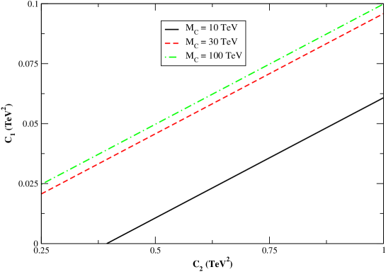
Figure 1: Values of $c_{1}$ and $c_{2}$ consistent with the correct value of $\tan\theta_{W}$ for different choices of the compactification scale $M_{C}$. We use $\tan\theta_{W}=0.54839$ in these results [26].

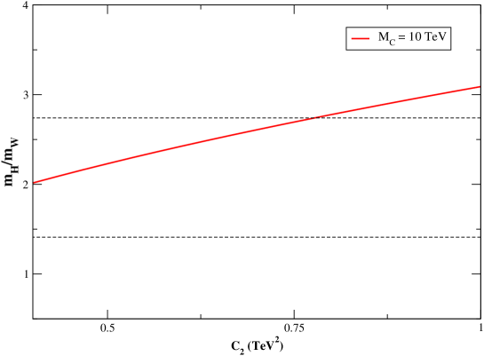
Figure 2: $m_{H}/m_{w}$ obtained with the values of $c_{1}$ and $c_{2}$ in fig. 1 for $M_{C}=10$ TeV. The horizontal lines correspond to the range consistent with global fits.

This example shows that it is possible to fix the problem in the original model by introducing brane kinetic terms as in (20). As discussed above, we introduced brane kinetic terms only for the 6D gauge components that turn into 4D gauge components. Apart from simplicity, our goal was to relate these terms to the value of $\tan\theta_{W}$ without disturbing the original tree level scalar potential. However, brane kinetic terms for the gauge-scalar components can also be incorporated and will cause modifications to the classical scalar potential [25].

4 Conclusion

In order to solve the little hierarchy problem it is possible to identify the Higgs field with components of gauge fields in higher dimensional electroweak theories. One such extended electroweak theory was presented by Scrucca et. al. in [16], where an SU(3) gauge theory in six dimensions is acted upon by an orbifold in such a way that one obtains a Higgs doublet in the low-energy effective theory. The model predicts $m_{H}=2m_{W}$, which is in the range suggested by global fits, and $\tan\theta_{W}=\sqrt{3}$ which is larger than the measured value. In this letter we presented a modification of the model in [16] that fixed the prediction of the Weinberg angle while keeping the results in the Higgs sector. We accomplished this by introducing brane kinetic terms in the 6D theory with different strengths for the already (orbifold) differentiated components of the gauge fields.

References

- [1] I. Gogoladze, T. j. Li, Y. Mimura and S. Nandi, “Orbifold unification for the gauge and Higgs fields and their couplings,” Phys. Lett. B 622, 320 (2005) [arXiv:hep-ph/0501264].
- [2] K. Choi, K. S. Jeong, T. Kobayashi and K. i. Okumura, “Little SUSY hierarchy in mixed modulus-anomaly mediation,” arXiv:hep-ph/0508029.
- [3] R. Dermisek and J. F. Gunion, “Escaping the large fine tuning and little hierarchy problems in the next to minimal supersymmetric model and h a a decays,” Phys. Rev. Lett. 95, 041801 (2005) [arXiv:hep-ph/0502105].
- [4] A. Birkedal, Z. Chacko and M. K. Gaillard, “Little supersymmetry and the supersymmetric little hierarchy problem,” JHEP 0410, 036 (2004) [arXiv:hep-ph/0404197].
- [5] H. C. Cheng and I. Low, “Little hierarchy, little Higgses, and a little symmetry,” JHEP 0408, 061 (2004) [arXiv:hep-ph/0405243].
- [6] H. C. Cheng and I. Low, “TeV symmetry and the little hierarchy problem,” JHEP 0309, 051 (2003) [arXiv:hep-ph/0308199].
- [7] J. G. Wacker, “Little Higgs models: New approaches to the hierarchy problem,” arXiv:hep-ph/0208235.
- [8] N. S. Manton, “A New Six-Dimensional Approach To The Weinberg-Salam Model,” Nucl. Phys. B 158, 141 (1979).
- [9] D. B. Fairlie, “Higgs’ Fields And The Determination Of The Weinberg Angle,”
- [10] H. Hatanaka, T. Inami and C. S. Lim, “The gauge hierarchy problem and higher dimensional gauge theories,” Mod. Phys. Lett. A 13, 2601 (1998) [arXiv:hep-th/9805067].
- [11] G. R. Dvali, S. Randjbar-Daemi and R. Tabbash, “The origin of spontaneous symmetry breaking in theories with large extra dimensions,” Phys. Rev. D 65, 064021 (2002) [arXiv:hep-ph/0102307].
- [12] N. Arkani-Hamed, A. G. Cohen and H. Georgi, “Electroweak symmetry breaking from dimensional deconstruction,” Phys. Lett. B 513, 232 (2001) [arXiv:hep-ph/0105239].
- [13] I. Antoniadis, K. Benakli and M. Quiros, “Finite Higgs mass without supersymmetry,” New J. Phys. 3, 20 (2001) [arXiv:hep-th/0108005].
- [14] C. Csaki, C. Grojean and H. Murayama, “Standard model Higgs from higher dimensional gauge fields,” Phys. Rev. D 67, 085012 (2003) [arXiv:hep-ph/0210133].
- [15] C. A. Scrucca, M. Serone and L. Silvestrini, “Electroweak symmetry breaking and fermion masses from extra dimensions,” Nucl. Phys. B 669, 128 (2003) [arXiv:hep-ph/0304220].
- [16] C. A. Scrucca, M. Serone, L. Silvestrini and A. Wulzer, “Gauge-Higgs unification in orbifold models,” JHEP 0402, 049 (2004) [arXiv:hep-th/0312267].
- [17] A. Wulzer, “Gauge-Higgs unification in six dimensions,” arXiv:hep-th/0405168.
- [18] C. Biggio and M. Quiros, “Higgs-gauge unification without tadpoles,” Nucl. Phys. B 703, 199 (2004) [arXiv:hep-ph/0407348].
- [19] M. Serone, “The Higgs boson as a gauge field in extra dimensions,” arXiv:hep-ph/0508019. Phys. Lett. B 82, 97 (1979).
- [20] J. L. Diaz-Cruz, “Tracing the gauge origin of Yukawa and Higgs parameters beyond the standard model,” Mod. Phys. Lett. A 20, 2397 (2005) [arXiv:hep-ph/0409216]; A. Aranda, J. L. Diaz-Cruz and A. Rosado, “Electroweak - Higgs unification and the Higgs boson mass,” arXiv:hep-ph/0507230.
- [21] F. del Aguila, M. Perez-Victoria and J. Santiago, “Bulk fields with general brane kinetic terms,” JHEP 0302, 051 (2003) [arXiv:hep-th/0302023].
- [22] M. Carena, E. Ponton, T. M. P. Tait and C. E. M. Wagner, “Opaque branes in warped backgrounds,” Phys. Rev. D 67, 096006 (2003) [arXiv:hep-ph/0212307].
- [23] H. Davoudiasl, J. L. Hewett, B. Lillie and T. G. Rizzo, “Warped Higgsless models with IR-brane kinetic terms,” JHEP 0405, 015 (2004) [arXiv:hep-ph/0403300].
- [24] M. Chaichian and A. Kobakhidze, “Kaluza-Klein decomposition and gauge coupling unification in orbifold GUTs,” arXiv:hep-ph/0208129.
- [25] Work in progress.
- [26] S. Eidelman et al., Phys. Lett. B 592, 1 (2004).
- [27] A. Aranda, C. Balazs and J. L. Diaz-Cruz, “Where is the Higgs boson? ((V)),” Nucl. Phys. B 670, 90 (2003) [arXiv:hep-ph/0212133]; J. L. Diaz-Cruz and D. A. Lopez-Falcon, “Probing the mechanism of EWSB with a rho parameter defined in terms of Higgs couplings,” Phys. Lett. B 568, 245 (2003) [arXiv:hep-ph/0304212].