Abstract

We consider the QCD corrections to the electric dipole moment of the neutron in the Minimal Supersymmetric Standard Model. We provide a master formula for the Wilson coefficients at the low energy scale including for the first time the mixing between the electric and chromoelectric operators and correcting widely used previous LO estimates. We show that, because of the mixing between the electric and chromoelectric operators, the neutralino contribution is always strongly suppressed. We find that, in general, the effect of the QCD corrections is to reduce the amount of CP violation generated at the high scale. We discuss the perturbative uncertainties of the LO computation, which are particularly large for the gluino-mediated contribution. This motivates our Next-to-Leading order analysis. We compute for the first time the order $\alpha_{s}$ corrections to the Wilson coefficients for the gluino contributions, and recompute the two-loop anomalous dimension for the dipole operators. We show that the large LO uncertainty disappears once NLO corrections are taken into account.

1 Introduction

CP violation plays a twofold role in SUSY model building. On the one hand, it is one of the main motivations to invoke New Physics (NP), since within the Standard Model (SM) it is not possible to construct a successful theory of baryogenesis, and also in the Minimal Supersymmetric Standard Model (MSSM) electroweak baryogenesis calls for additional sources of CP violation beyond the SM single phase in the Cabibbo-Kobayashi-Maskawa (CKM) quark mixing matrix [1]. On the other hand, CP violating processes provide very stringent constraints on NP. Indeed, the recent experimental progress in the study of FCNC processes allows us to conclude that most probably NP cannot contribute substantially (i.e. more than $\sim 20-30\%$) to flavour and CP violation in $\Delta S=2$ and $\Delta B=2$ processes [2]. Since the MSSM contains tens of new sources of flavour and CP violation, this experimental observation is quite puzzling, leading to the so-called SUSY flavour problem, which is one of the main open issues in SUSY model building [3].

The new sources of CP violation present in the MSSM can be divided in two groups: the first one contains new phases that appear in flavour conserving quantities, the second contains those new sources of CP violation that are also new sources of flavour violation. While the latter are strongly constrained by $K$ and $B$ physics, at least for those flavour-changing parameters that connect the first generation to the other two, the new sources of CP violation that are not directly connected to flavour violation have little impact on FCNC processes [4] and are mainly constrained by the Electric Dipole Moments (EDM) of the electron and of the neutron [5, 6, 7]. A careful analysis of EDM processes is therefore mandatory in order to assess the allowed size of these NP contributions to CP violation and their possible effects in electroweak baryogenesis and in other CP violating processes.

Surprisingly enough, while the study of FCNC processes in the MSSM has recently witnessed considerable theoretical advances, with the inclusion of Next-to-Leading Order (NLO) QCD corrections [8] and with the computation of the relevant hadronic matrix elements with Lattice QCD [9], not only no corresponding effort has been made in the study of the EDM of the neutron, but even incorrect LO results have been widely used in the literature.

The present work aims to be a first step towards bringing the EDM analysis in SUSY at the same level of accuracy as the other FCNC and CP violation studies. In particular, we focus on the perturbative aspects of the QCD corrections to the neutron EDM.

The paper is organized as follows. In section 2 we discuss the neutron EDM at the LO in QCD: we give a complete LO formula for the EDM, correcting some errors in previous analyses, and we discuss the interplay of the various contributions. We then study the uncertainties related to the LO approximation, and we find that they are particularly large for gluino contributions. This motivates us to upgrade the analysis to NLO that is presented in the next section. We introduce the NLO QCD evolution and the NLO matching conditions for the gluino contribution. We show that after the inclusion of the NLO contributions the scale uncertainty is reduced down to $\sim 2.5\%$. Finally we present some conclusions.

2 Leading Order Analysis

In this Section, we provide the full LO expressions for the neutron EDM in the MSSM, we discuss the interplay of the various SUSY contributions and we study the uncertainties of the LO approximation.

2.1 Anomalous dimension

We write the relevant CP-violating effective low-energy Hamiltonian as

$$H_{CPV}=\sum_{q}C_{1}^{q}(\mu)O_{1}^{q}(\mu)+\sum_{q}C_{2}^{q}(\mu)O_{2}^{q}(\mu)+C_{3}(\mu)O_{3}(\mu)~{}~{},$$ (1)

where

$$O_{1}^{q} = -\frac{i}{2}e\,Q_{q}m_{q}\,\bar{q}\sigma^{\mu\nu}\gamma_{5}q\,F_{\mu\nu},$$

$$O_{2}^{q} = -\frac{i}{2}g_{s}m_{q}\bar{q}\,\sigma^{\mu\nu}t^{a}\gamma_{5}q\,G^{a}_{\mu\nu},$$

$$O_{3} = -\frac{1}{6}g_{s}f^{abc}G^{a}_{\mu\rho}G^{b\rho}_{\nu}G^{c}_{\lambda\sigma}\epsilon^{\mu\nu\lambda\sigma}\,.$$ (2)

The index $q$ runs over light quarks, and $Q_{q}=(2/3,-1/3)$ for up- and down-type quarks respectively. With this choice, all the operators have dimension six.

Defining $\vec{C}=(C_{1}^{q},C_{2}^{q},C_{3})$ we write the renormalization group equation for the Wilson coefficients as:

$$\frac{d\,\vec{C}(\mu)}{d\,\ln\mu}=\gamma^{T}\vec{C}(\mu)$$ (3)

where at the LO $\gamma(\alpha_{s})=(\alpha_{s}/4\pi)\,\gamma^{(0)}$.

Let us now discuss the LO anomalous dimensions of the operators in eq. (2). The anomalous dimensions of operators $O_{1}^{q}$ and $O_{2}^{q}$ can be easily gleaned from that of the operators $O_{7}$ and $O_{8}$ relevant in the $b\to s\gamma$ process (see ref. [10]). The anomalous dimension of the Weinberg operator $O_{3}$ [11] and of its mixing with $O_{2}$ was derived in ref. [12]. Therefore we get the following LO anomalous dimension matrix:

$$\gamma^{(0)}\equiv\left(\begin{array}[]{ccc}\gamma_{e}&0&0\\ &\\ \gamma_{qe}&\gamma_{q}&0\\ &\\ 0&\gamma_{{\scriptscriptstyle G}q}&\gamma_{\scriptscriptstyle G}\end{array}\right)=\left(\begin{array}[]{ccc}8\,C_{F}&0&0\\ &\\ 8\,C_{F}&16\,C_{F}-4\,N&0\\ &\\ 0&-2\,N&N+2n_{f}+\beta_{0}\end{array}\right)$$ (4)

where $C_{F}=4/3,\,N=3,\,\beta_{0}=\frac{1}{3}(11N-2n_{f})$ with $n_{f}$ the number of active flavours. The Wilson coefficients at the hadronic scale $\mu_{H}$ can be easily obtained from those at a high scale $\mu_{\rm S}$ from

$$C_{1}^{q}(\mu_{H}) = {\eta}^{\kappa_{e}}C_{1}^{q}(\mu_{\rm S})+\frac{\gamma_{qe}}{\gamma_{e}-\gamma_{q}}\left({\eta}^{\kappa_{e}}-{\eta}^{\kappa_{q}}\right)\,C_{2}^{q}(\mu_{\rm S})+$$ (5)

$$\left[\frac{\gamma_{{\scriptscriptstyle G}q}\gamma_{qe}\,{\eta}^{\kappa_{e}}}{(\gamma_{q}-\gamma_{e})(\gamma_{{\scriptscriptstyle G}}-\gamma_{e})}+\frac{\gamma_{{\scriptscriptstyle G}q}\gamma_{qe}\,{\eta}^{\kappa_{q}}}{(\gamma_{e}-\gamma_{q})(\gamma_{{\scriptscriptstyle G}}-\gamma_{q})}+\frac{\gamma_{{\scriptscriptstyle G}q}\gamma_{qe}\,\eta^{\kappa_{{\scriptscriptstyle G}}}}{(\gamma_{e}-\gamma_{{\scriptscriptstyle G}})(\gamma_{q}-\gamma_{{\scriptscriptstyle G}})}\right]\,C_{3}(\mu_{\rm S})~{},$$

$$C_{2}^{q}(\mu_{H}) = {\eta}^{\kappa_{q}}C_{2}^{q}(\mu_{\rm S})+\frac{\gamma_{{\scriptscriptstyle G}q}}{\gamma_{q}-\gamma_{{\scriptscriptstyle G}}}\left({\eta}^{\kappa_{q}}-{\eta}^{\kappa_{{\scriptscriptstyle G}}}\right)\,C_{3}(\mu_{\rm S})~{},$$ (6)

$$C_{3}(\mu_{H}) = {\eta}^{\kappa_{{\scriptscriptstyle G}}}C_{3}(\mu_{\rm S})~{},$$ (7)

where $\eta=\alpha_{s}(\mu_{\rm S})/\alpha_{s}(\mu_{H})$ and $\kappa_{i}=\gamma_{i}/(2\beta_{0})$.

The operator basis in eq. (2) is very suitable to discuss the anomalous dimension matrix. However, in order to avoid the explicit appearance of the strong coupling at the low scale in the operators, it is more convenient to introduce a slightly different operator basis

$$O_{e}^{q} = -\frac{i}{2}e\,Q_{q}m_{q}\,\bar{q}\sigma^{\mu\nu}\gamma_{5}q\,F_{\mu\nu},$$

$$O_{c}^{q} = -\frac{i}{2}m_{q}\bar{q}\,\sigma^{\mu\nu}t^{a}\gamma_{5}q\,G^{a}_{\mu\nu},$$

$$O_{\scriptscriptstyle G} = -\frac{1}{6}f^{abc}G^{a}_{\mu\rho}G^{b\rho}_{\nu}G^{c}_{\lambda\sigma}\epsilon^{\mu\nu\lambda\sigma}$$ (8)

that defines our electric dipole ($O_{e}$), chromoelectric dipole ($O_{c}$) and Weinberg operator ($O_{\scriptscriptstyle G}$) and whose corresponding Wilson coefficients can be easily obtained from eqs. (5–7) by redefining the coefficients as follows:

$$g_{s}(\mu_{H})\,C_{2}^{q}(\mu_{\rm S}) = \eta^{-(1/2)}C_{c}^{q}(\mu_{\rm S}),$$

$$g_{s}(\mu_{H})\,C_{3}(\mu_{\rm S}) = \eta^{-(1/2)}C_{\scriptscriptstyle G}(\mu_{\rm S}).$$ (9)

To illustrate in a simple way the relation between the Wilson coefficients at the $\mu_{\rm S}$ scale and those at the $\mu_{H}$ scale we take $\mu_{\rm S}\sim m_{t}$ and assume five flavours of light quarks between the scales $\mu_{\rm S}$ and $\mu_{H}$, obtaining

$$C_{e}^{q}(\mu_{H}) = {\eta}^{{16\over 23}}C_{e}^{q}(\mu_{\rm S})+8\left({\eta}^{{16\over 23}}-{\eta}^{{14\over 23}}\right)\,{C_{c}^{q}(\mu_{\rm S})\over g_{s}(\mu_{\rm S})}\mathbf{+}\frac{24}{85}\left[17\,{\eta}^{{16\over 23}}-15\,{\eta}^{{14\over 23}}-2\,{\eta}^{{31\over 23}}\right]\,{C_{\scriptscriptstyle G}(\mu_{\rm S})\over g_{s}(\mu_{\rm S})},$$ (10)

$$C_{c}^{q}(\mu_{H}) = {\eta}^{{5\over 46}}C_{c}^{q}(\mu_{\rm S})+\frac{9}{17}\left({\eta}^{{5\over 46}}-{\eta}^{{39\over 46}}\right)\,C_{\scriptscriptstyle G}(\mu_{\rm S}),$$ (11)

$$C_{\scriptscriptstyle G}(\mu_{H}) = {\eta}^{{39\over 46}}C_{\scriptscriptstyle G}(\mu_{\rm S}).$$ (12)

It is interesting to note that in eqs. (10–12) all the $\eta$’s are raised to a positive power and then act as suppression factors.

$X_{11}^{23}$	$1.25857$	$X_{12}^{12}$	$-9.78321$	$X_{12}^{23}$	$10.06853$
$X_{13}^{12}$	$-4.63415$	$X_{13}^{23}$	$5.33040$	$X_{13}^{35}$	$-1.60476$
$X_{13}^{43}$	$7.76606$	$X_{13}^{52}$	$-7.05911$	$X_{22}^{11}$	$1.22290$
$X_{23}^{11}$	$0.57927$	$X_{23}^{34}$	$-1.30387$	$X_{23}^{51}$	$0.88239$
$X_{33}^{34}$	$2.17311$

Table 1: Magic numbers $X_{ij}^{ab}$ for the evolution from six to four flavours. See the text for details.

In general, SUSY masses are expected to be above $m_{t}$ while the hadronic matrix element is evaluated at a scale of the order of the neutron mass. In this situation it is more appropriate to consider the evolution from $\mu_{\rm S}>m_{t}$ to $\mu_{H}<m_{b}$, i.e. from the six- to the four-flavour theory, that can be summarized via the so-called “magic numbers”. In this case, the low-energy coefficients $\vec{\rm C}(\mu_{H})\equiv(C_{e}^{q},C_{c}^{q},C{\scriptscriptstyle G})$ are given in terms of the high energy ones as

$${\rm C}_{i}(\mu_{H})=\sum_{j=1}^{3}\sum_{a,b=1}^{5}X_{ij}^{ab}\alpha_{s}(\mu_{\rm S})^{Y_{a}}\eta^{Z_{b}}g_{s}(\mu_{\rm S})^{\delta_{i1}(\delta_{j1}-1)}{\rm C}_{j}(\mu_{\rm S})\,,$$ (13)

with $Y_{a}$ and $Z_{b}$ given by:

$$Y_{a} = \left\{\frac{8}{75},\frac{64}{525},\frac{72}{175},\frac{163}{175},\frac{177}{175}\right\},$$

$$Z_{b} = \left\{\frac{3}{50},\frac{14}{25},\frac{16}{25},\frac{33}{50},\frac{29}{25}\right\}$$ (14)

and the nonvanishing entries in $X_{ij}^{ab}$ are listed in Table 1. These magic numbers have been obtained using the average values $\overline{m}_{t}(m_{t})=168.5$ GeV, $\overline{m}_{b}(m_{b})=4.28$ GeV and $\alpha_{s}(M_{Z})=0.119$.

A comparison with previous evaluations of the LO anomalous dimension matrix is now in order. Several partial LO results are present in the literature [13, 14, 12, 15] although the work of ref. [15], to be called ALN, can be regarded as the standard reference for the QCD correction to the neutron EDM with its numerical estimates of the QCD correction factors that have been and are still widely used. With respect to ALN our analysis differs in two aspects: i) we have included the mixing between the operators $O_{e}$ and $O_{c}$ that is neglected in ALN. ii) Our definition of the operator basis (eq. (8)) is different from that employed in ALN. In particular, we write explicitly in the definition of the operators $O_{e}$ and $O_{c}$ the mass of the quark, as well as in $O_{e}$ the charge of quark, while in the operator basis of ALN the quark mass and charge is not present. Correspondingly the anomalous dimension matrix of ALN should differ from ours by a factor $\gamma_{m}=-6\,C_{F}$. Taking into account this difference we find agreement with ALN in the anomalous dimension result for the chromoelectric and Weinberg operators. Instead, for the electric dipole operator we find that, with the conventions employed by ALN, the anomalous dimension should read $\gamma_{e}=-8/3$ , i.e. it has the opposite sign with respect to the one quoted in ref. [15]. As a consequence, the QCD renormalization factor of the dipole operator, $\eta^{\rm ED}$, that is estimated in ALN to be $\eta^{\rm ED}=1.53$, should be $\eta^{\rm ED}<1$ , i.e it does not enhance the CP violating effect but actually suppresses it. Employing the same values for strong coupling at the high and low scale used in ALN we get $\eta^{\rm ED}\sim 0.61$.

In our view the definition of the operator basis we employ (eq. (8)) has the advantage to make more transparent the behavior of the perturbative QCD corrections to the neutron EDM that in general give correction factors that decrease the amount of CP violation generated at the high scale. In the ALN operator basis this effect is somewhat hidden by the fact that the quark mass entering their Wilson coefficients has to be taken at the high scale and $m_{q}(\mu_{\rm S})<m_{q}(\mu_{H})$. It should be noticed that the dependence of the Wilson coefficients upon the quark mass can also appear in an indirect way, e.g. through the matrices that diagonalize squark masses.

2.2 Hadronic Matrix Elements

In order to compute the EDM of the neutron the matrix elements of $O_{e}^{q},\,O_{c}^{q},\,O_{\scriptscriptstyle G}$ between neutron states are also needed. At the moment a result from Lattice QCD is not yet available, although first steps in this direction have been recently made [16]. Several alternative approaches have been used to estimate these matrix elements, as QCD sum rules [17] or chiral Lagrangians [18]. In this paper we are mainly concerned about perturbative aspects of the EDM calculation, thus we are going to use the simplest estimates of the operator matrix elements. In particular, for the electric dipole operator, we use the chiral quark model where the neutron is seen as a collection of three valence quarks described by an $SU(6)$ symmetric spin-flavour wave function. In this model the neutron EDM is related to that of the valence quarks by

$$d^{e}_{n}=\frac{1}{3}\left(4d^{e}_{d}-d^{e}_{u}\right),$$ (15)

where

$$d^{e}_{q}=e\,Q_{q}\,m_{q}(\mu_{H})\,C^{q}_{e}(\mu_{H})$$ (16)

is the quark EDM. Concerning the contribution of the chromoelectric and Weinberg operators to $d_{n}$ the simplest estimate is obtained via naive dimensional analysis [19] giving

$$d^{c}_{n} = \frac{e}{4\pi}\,\left(m_{u}(\mu_{H})\,C^{c}_{u}(\mu_{H})+m_{d}(\mu_{H})\,C^{c}_{d}(\mu_{H})\right),$$ (17)

$$d^{\scriptscriptstyle G}_{n} = \frac{e}{4\pi}\,\Lambda\,C_{\scriptscriptstyle G}(\mu_{H})$$ (18)

where $\Lambda\approx 1.19$ GeV is the chiral-symmetry-breaking scale. We notice that in eqs. (16) and (17) $m_{q}$ is computed at the hadronic scale, while in the expressions for the Wilson coefficients at the $\mu_{\rm S}$ scale the masses, as well as $g_{s}$, are computed at the high scale.

2.3 Wilson Coefficients in the MSSM

The discussion in the previous sections has been general and applies to any model in which $CP$ violating effects are generated at some high scale. In this section we focus on the minimal supersymmetric standard model (MSSM) with complex parameters assuming also that the trilinear SUSY-breaking scalar couplings are proportional to the corresponding Yukawa coupling. In this model besides the SM $CP$ violating phases $(\delta_{CKM},\,\theta_{QCD})$ that will be neglected in the present discussion as well as the flavour mixing, there are new phases associated to the $\mu$-term in the superpotential, the supersymmetry-breaking parameters of the gaugino mass, the trilinear scalar couplings $A$, and the bilinear scalar term in the Higgs potential. However not all the phases of these quantities are physical. It is then possible to assume the gaugino masses and the bilinear term to be real so that we are left only with two $CP$ violating phases, one associated with the $\mu$ term, $(\phi_{\mu})$, and the other with the trilinear scalar coupling, $(\phi_{A})$, that is in general flavour-dependent. These phases will be present in the mass matrices of squarks, charginos and neutralinos inducing an EDM at the quark level. In particular in the squark mass matrix

$$M^{2}_{\tilde{q}}=\left(\begin{array}[]{cc}m_{\tilde{q}_{L}}^{2}&m_{q}X_{q}\\ m_{q}X_{q}^{\ast}&\,m_{\tilde{q}_{R}}^{2}\end{array}\right)$$ (19)

the only complex parameter is the left-right mixing term $X_{u}\equiv A^{\ast}_{u}-\mu\cot\beta,\>X_{d}\equiv A^{\ast}_{d}-\mu\tan\beta$, where both phases are present. In $X_{q}$, $\tan\beta=v_{2}/v_{1}$ is the ratio of the VEVs of the Higgs fields. Instead in the chargino mass matrix

$$M_{\tilde{C}}=\left(\begin{array}[]{cc}M_{2}&\sqrt{2}\,s_{\beta}\,M_{W}\\ \sqrt{2}\,c_{\beta}\,M_{W}&\mu\end{array}\right)$$ (20)

as well as in the neutralino one

$$M_{\tilde{N}}=\left(\begin{array}[]{cccc}M_{1}&0&-c_{\beta}\,s_{W}\,M_{Z}&s_{\beta}\,s_{W}\,M_{Z}\\ 0&M_{2}&c_{\beta}\,c_{W}\,M_{Z}&-s_{\beta}\,c_{W}\,M_{Z}\\ -c_{\beta}\,s_{W}\,M_{Z}&c_{\beta}\,c_{W}\,M_{Z}&0&-\mu\\ s_{\beta}\,s_{W}\,M_{Z}&-s_{\beta}\,c_{W}\,M_{Z}&-\mu&0\end{array}\right)$$ (21)

the only complex term is $\mu$ and therefore only $\phi_{\mu}$ is present. In eqs. (20,21) $s_{\beta}\equiv\sin\beta,\,c_{\beta}\equiv\cos\beta$, $s_{W}$, $c_{W}$ are the sine and cosine of the weak mixing angle and $M_{1,2}$ are the soft-breaking gaugino masses associated to the $U(1)$ and $SU(2)$ groups.

To present our results in a transparent way we perform the computation of the Wilson coefficients using current eigenstates for squark fields. In this basis the squark propagator is a $2\times 2$ matrix given by

$$\Delta_{\tilde{q}}(k)=\frac{i}{(k^{2}-m_{\tilde{q}_{1}}^{2})\,(k^{2}-m_{\tilde{q}_{2}}^{2})}\,\left(\begin{array}[]{cc}k^{2}-m_{\tilde{q}_{R}}^{2}&m_{q}X_{q}^{\ast}\\ m_{q}X_{q}&k^{2}-m_{\tilde{q}_{L}}^{2}\end{array}\right)$$ (22)

where $m_{\tilde{q}_{i}}$ are the eigenvalues of $M^{2}_{\tilde{q}}$. Neglecting ${\cal O}(m_{q}^{2})$ terms we have that $m_{\tilde{q}_{1}}\simeq m_{\tilde{q}_{L}},\,m_{\tilde{q}_{2}}\simeq m_{\tilde{q}_{R}}$ so that $\Delta_{\tilde{q}}(k)$ reduces to

$$\Delta_{\tilde{q}}(k)\simeq\,i\,\left(\begin{array}[]{cc}\frac{1}{k^{2}-m_{\tilde{q}_{1}}^{2}}&\frac{m_{q}X_{q}^{\ast}}{(k^{2}-m_{\tilde{q}_{1}}^{2})\,(k^{2}-m_{\tilde{q}_{2}}^{2})}\\ \frac{m_{q}X_{q}}{(k^{2}-m_{\tilde{q}_{1}}^{2})\,(k^{2}-m_{\tilde{q}_{2}}^{2})}&\frac{1}{k^{2}-m_{\tilde{q}_{2}}^{2}}\end{array}\right).$$ (23)

We notice that within this approximation the left-right propagator is still exact.

The Wilson coefficients of the operators $O_{e},\,O_{c}$ are generated at the one-loop order while that of $O_{\scriptscriptstyle G}$ appears for the first time at the two-loop level. At the LO we can then set $C_{\scriptscriptstyle G}(\mu_{\rm S})=0$ and write

$$C_{e}^{q}(\mu_{\rm S})=C_{e\tilde{g}}^{q}(\mu_{\rm S})+C_{e\tilde{\chi}^{-}}^{q}(\mu_{\rm S})+C_{e\tilde{\chi}^{0}}^{q}(\mu_{\rm S})$$ (24)

and similarly for $C_{c}^{q}$.

We find for the gluino contribution

$$C_{e\tilde{g}}^{q}(\mu_{\rm S}) = \frac{\alpha_{s}}{4\pi\,m_{\tilde{g}}^{2}}{\rm Im}\left(\frac{X_{q}}{m_{\tilde{g}}}\right){8\over 3}\,\tilde{B}\left(x_{1},x_{2}\right),$$ (25)

$$C_{c\tilde{g}}^{q}(\mu_{\rm S}) = \frac{g_{s}\,\alpha_{s}}{4\pi\,m_{\tilde{g}}^{2}}{\rm Im}\left(\frac{X_{q}}{m_{\tilde{g}}}\right)\,\tilde{C}\left(x_{1},x_{2}\right)$$ (26)

where $x_{i}=m_{\tilde{g}}^{2}/m_{\tilde{q}_{i}}^{2}$. The explicit expressions for the functions $\tilde{B}$ and $\tilde{C}$ as well as those entering in the chargino and neutralino contributions are collected in the Appendix.

For the chargino we have

$$C_{e\tilde{\chi}^{-}}^{u}(\mu_{\rm S}) = \frac{\alpha\,Q_{u}^{-1}}{4\pi s^{2}_{W}}\,\sum_{i=1}^{2}\frac{1}{\sqrt{2}\,s_{\beta}\,\,m_{\tilde{\chi_{i}}^{-}}^{2}}\,\left(\frac{\,m_{\tilde{\chi_{i}}^{-}}}{M_{W}}\right)\,\left\{{\rm Im}\left(V_{i2}\,U_{i1}\right)\left[(Q_{d}-Q_{u})\,A(y_{\tilde{d}_{1}}^{i})+Q_{d}\,B(y_{\tilde{d}_{1}}^{i})\right]\right.$$ (27)

$$\left.~{}~{}~{}~{}-{\rm Im}\left(\frac{m_{d}X_{d}^{\ast}}{m_{\tilde{\chi_{i}}^{-}}^{2}}V_{i2}\,U_{i2}\right)Y_{d}\left[(Q_{d}-Q_{u})\,\tilde{A}(y_{\tilde{d}_{1}}^{i},y_{\tilde{d}_{2}}^{i})+Q_{d}\,\tilde{B}(y_{\tilde{d}_{1}}^{i},y_{\tilde{d}_{2}}^{i})\right]\right\},$$

$$C_{e\tilde{\chi}^{-}}^{d}(\mu_{\rm S}) = \frac{\alpha\,Q_{d}^{-1}}{4\pi s^{2}_{W}}\,\sum_{i=1}^{2}\frac{1}{\sqrt{2}\,c_{\beta}\,\,m_{\tilde{\chi_{i}}^{-}}^{2}}\,\left(\frac{\,m_{\tilde{\chi_{i}}^{-}}}{M_{W}}\right)\,\left\{{\rm Im}\left(V_{i1}\,U_{i2}\right)\left[(Q_{u}-Q_{d})\,A(y_{\tilde{u}_{1}}^{i})+Q_{u}\,B(y_{\tilde{u}_{1}}^{i})\right]\right.$$ (28)

$$\left.~{}~{}~{}~{}-{\rm Im}\left(\frac{m_{u}X_{u}^{\ast}}{m_{\tilde{\chi_{i}}^{-}}^{2}}V_{i2}\,U_{i2}\right)Y_{u}\left[(Q_{u}-Q_{d})\,\tilde{A}(y_{\tilde{u}_{1}}^{i},y_{\tilde{u}_{2}}^{i})+Q_{u}\,\tilde{B}(y_{\tilde{u}_{1}}^{i},y_{\tilde{u}_{2}}^{i})\right]\right\},$$

$$C_{c\tilde{\chi}^{-}}^{u}(\mu_{\rm S}) = \frac{g_{s}\,\alpha}{4\pi s^{2}_{W}}\,\sum_{i=1}^{2}\frac{1}{\sqrt{2}\,s_{\beta}\,\,m_{\tilde{\chi_{i}}^{-}}^{2}}\,\left(\frac{\,m_{\tilde{\chi_{i}}^{-}}}{M_{W}}\right)\,\left\{{\rm Im}\left(V_{i2}\,U_{i1}\right)B(y_{\tilde{d}_{1}}^{i})\right.$$ (29)

$$\left.~{}~{}~{}~{}-{\rm Im}\left(\frac{m_{d}X_{d}^{\ast}}{m_{\tilde{\chi_{i}}^{-}}^{2}}V_{i2}\,U_{i2}\right)Y_{d}\tilde{B}(y_{\tilde{d}_{1}}^{i},y_{\tilde{d}_{2}}^{i})\right\},$$

$$C_{c\tilde{\chi}^{-}}^{d}(\mu_{\rm S}) = \frac{g_{s}\,\alpha}{4\pi s^{2}_{W}}\,\sum_{i=1}^{2}\frac{1}{\sqrt{2}\,c_{\beta}\,\,m_{\tilde{\chi_{i}}^{-}}^{2}}\,\left(\frac{\,m_{\tilde{\chi_{i}}^{-}}}{M_{W}}\right)\,\left\{{\rm Im}\left(V_{i1}\,U_{i2}\right)B(y_{\tilde{u}_{1}}^{i})\right.$$ (30)

$$\left.~{}~{}~{}~{}-{\rm Im}\left(\frac{m_{u}X_{u}^{\ast}}{m_{\tilde{\chi_{i}}^{-}}^{2}}V_{i2}\,U_{i2}\right)Y_{u}\tilde{B}(y_{\tilde{u}_{1}}^{i},y_{\tilde{u}_{2}}^{i})\right\}$$

where $y_{\tilde{q}_{j}}^{i}=m_{\tilde{\chi}^{-}_{i}}^{2}/m_{\tilde{q}_{j}}^{2}$, $U$ and $V$ are the matrices that diagonalize $M_{\tilde{C}}$ according to $U^{\ast}M_{\tilde{C}}V^{-1}=M_{\tilde{C}}^{D}$ and $Y_{u,d}$ are the Yukawa couplings of the up and down quarks in units of $e/s_{W}$. In eqs. (27–30) we have also written explicitly the contributions proportional to the mass and the Yukawa coupling of the light quarks to show that the phase combination that enters in the gluino contribution is actually present in the chargino term in a suppressed way. Indeed, in the chargino contribution the only relevant phase is $\phi_{\mu}$, hidden inside the matrices $U$ and $V$. This can be seen explicitly in the following simplified expression, obtained by neglecting the contributions proportional to quark masses and Yukawa couplings:

$$C_{e\tilde{\chi}^{-}}^{u}(\mu_{\rm S}) = \frac{\alpha\,Q_{u}^{-1}}{4\pi s^{2}_{W}}\,\sum_{i=1}^{2}\frac{1}{\sqrt{2}\,s_{\beta}\,\,m_{\tilde{\chi_{i}}^{-}}^{2}}\,\left\{{\rm Im}\left(\frac{U_{i2}^{*}\,U_{i1}\mu}{M_{W}}\right)\left[(Q_{d}-Q_{u})\,A(y_{\tilde{d}_{1}}^{i})+Q_{d}\,B(y_{\tilde{d}_{1}}^{i})\right]\right\}\,.$$

Analogous expressions can be obtained from eqs. (28)-(30) with the substitutions:

$$m_{\tilde{\chi_{i}}^{-}}\,{\rm Im}\left(V_{i2}\,U_{i1}\right) \to {\rm Im}\left(U_{i2}^{*}\,U_{i1}\mu\right)\,,$$

$$m_{\tilde{\chi_{i}}^{-}}\,{\rm Im}\left(V_{i1}\,U_{i2}\right) \to {\rm Im}\left(V_{i2}^{*}\,V_{i1}\mu\right)\,.$$ (32)

Finally the neutralino contribution, neglecting terms proportional to the the quark masses, is given by:

$$C_{e\tilde{\chi}^{0}}^{q}(\mu_{\rm S}) = \frac{\alpha}{4\pi s^{2}_{W}}\,\sum_{i=1}^{4}\frac{1}{\,m_{\tilde{\chi_{i}}^{0}}^{2}}\,\left\{{\rm Im}\left(\frac{K^{a}_{qi}K^{b}_{qi}X_{q}}{m_{\tilde{\chi}_{i}^{0}}}\right)\tilde{B}(z_{1}^{i},z_{2}^{i})\right.$$ (33)

$$\left.+\left(\frac{m_{\tilde{\chi_{i}}^{0}}}{M_{W}}\right)\,\left({\rm Im}\left(K^{b}_{qi}K^{c}_{qi}\right)B(z_{2}^{i})-{\rm Im}\left(K^{a}_{qi}K^{c}_{qi}\right)B(z_{1}^{i})\right)\right\},$$

$$C_{c\tilde{\chi}^{0}}^{q}(\mu_{\rm S}) = g_{s}\,C_{e\tilde{\chi}^{0}}^{q}$$ (34)

where $z_{j}^{i}=m_{\tilde{\chi}^{0}_{i}}^{2}/m_{\tilde{q}_{j}}^{2}$, and

$$K^{a}_{ui} = \sqrt{2}\left[\left(Q_{u}-\frac{1}{2}\right)\tan\theta_{W}\,Z^{i1}+\frac{1}{2}Z^{i2}\right]\,,$$ (35)

$$K^{b}_{ui} = \sqrt{2}\tan\theta_{W}\,Q_{u}\,Z^{i1}\,,$$ (36)

$$K^{c}_{ui} = \frac{1}{\sqrt{2}s_{\beta}}Z^{i4}\,,$$ (37)

$$K^{a}_{di} = \sqrt{2}\left[\left(Q_{d}+\frac{1}{2}\right)\tan\theta_{W}\,Z^{i1}-\frac{1}{2}Z^{i2}\right]\,,$$ (38)

$$K^{b}_{di} = \sqrt{2}\tan\theta_{W}\,Q_{d}\,Z^{i1}\,,$$ (39)

$$K^{c}_{di} = \frac{1}{\sqrt{2}c_{\beta}}Z^{i3}\,.$$ (40)

In eqs. (35-40) $Z$ is the matrix that diagonalizes $M_{\tilde{N}}$ according to $Z^{\ast}M_{\tilde{N}}Z^{-1}=M_{\tilde{N}}^{D}$. As can be seen from eq. (33) in the neutralino contribution both $\phi_{\mu}$, through the matrix $Z$, and the $X_{q}$ phase combination are actually present.

We noticed that the results reported in eqs. (25)-(30) and (33)-(40) are fully in agreement with those in ref. [5, 6] and represent the lowest order approximation.

2.4 LO results

In this section we investigate, at the LO, the effect of QCD corrections on the neutron EDM, to assess whether they can significantly reduce the individual gluino, chargino and neutralino contributions making the EDM constraint on SUSY phases less severe.

To discuss in a simple way the effect of the QCD corrections and in particular the importance of the mixing between $O_{e}$ and $O_{c}$ that was neglected in previous analyses, we consider eqs. (10-12) assuming $\eta=0.3$ and setting $C_{\scriptscriptstyle G}=0$. Then

$$C_{e}^{q}(\mu_{H}) = 0.43\,C_{e}^{q}(\mu_{\rm S})-0.38\,{C_{c}^{q}(\mu_{\rm S})\over g_{s}(\mu_{\rm S})},$$ (41)

$$C_{c}^{q}(\mu_{H}) = 0.88\,C_{c}^{q}(\mu_{\rm S}),$$ (42)

$$C_{\scriptscriptstyle G}(\mu_{H}) = 0.$$ (43)

Thus, if $C_{e}^{q}(\mu_{\rm S})\simeq C_{c}^{q}(\mu_{\rm S})/g_{s}(\mu_{\rm S})$ the resulting $C_{e}^{q}(\mu_{H})$ is strongly suppressed. With our definition of the operators the above situation is achieved when the gluon in a diagram contributing to $C_{c}^{q}$ is attached to a squark of the same charge of the external quark. This case is realized in the neutralino contribution (see eq. (34)). Indeed, we can estimate the neutralino contribution to $d_{n}^{e},\,d_{n}^{c}$, as given in eqs. (15,17), by employing the Wilson coefficient at the low scale evaluated via eqs. (10-12) with $g_{s}(\mu_{\rm S})=1.22$. We get

$$d_{n}^{e,\tilde{\chi}^{0}} \simeq \frac{e}{3}\left[4\,m_{d}(\mu_{H})\left(-\frac{1}{3}0.05\right)C_{e\tilde{\chi}^{0}}^{d}(\mu_{\rm S})-m_{u}(\mu_{H})\left(\frac{2}{3}0.05\right)C_{e\tilde{\chi}^{0}}^{u}(\mu_{\rm S})\right]$$ (44)

$$\approx e\left[-m_{d}(\mu_{H})\,0.02\,C_{e\tilde{\chi}^{0}}^{d}(\mu_{\rm S})-0.01\,m_{u}(\mu_{H})\,C_{e\tilde{\chi}^{0}}^{u}(\mu_{\rm S})\right]~{}~{},$$

$$d_{n}^{c,\tilde{\chi}^{0}} \simeq 0.88\frac{e}{4\pi}\left[m_{u}(\mu_{H})\,g_{s}(\mu_{\rm S})\,C_{e\tilde{\chi}^{0}}^{u}(\mu_{\rm S})+m_{d}(\mu_{H})\,g_{s}(\mu_{\rm S})\,C_{e\tilde{\chi}^{0}}^{d}(\mu_{\rm S})\right]$$ (45)

$$\approx e\,0.08\,\left[m_{u}(\mu_{H})\,C_{e\tilde{\chi}^{0}}^{u}(\mu_{\rm S})+m_{d}(\mu_{H})\,C_{e\tilde{\chi}^{0}}^{d}(\mu_{\rm S})\right].$$

Eqs. (44-45) show that the individual quark EDMs are strongly suppressed by the QCD corrections. A so large effect is actually specific to the neutralino contribution because of the simple relation between $C_{e\tilde{\chi}^{0}}^{q}$ and $C_{c\tilde{\chi}^{0}}^{q}$ (eq. (34)). The general case is more complicated and the resulting effect depends upon the relative sign between $C_{e}^{q}(\mu_{\rm S})$ and $C_{c}^{q}(\mu_{\rm S})$.

It is not our purpose here to perform a general analysis of EDM constraints on SUSY models. Rather, our aim is to illustrate the impact of QCD corrections on the computation of the EDM. To do so, we study a specific point in the SUSY parameter space that we choose with a mass spectrum similar to that of the benchmark point 1a of the Snowmass Points and Slopes (SPS) [20]. The SPS benchmark points are actually defined assuming real parameters, however we take the mass spectrum of point 1a as indicative, also in the case of complex parameters, of possible mass values of a “typical” mSUGRA scenario with an intermediate value of $\tan\beta$. We take $m_{\tilde{g}}=585$ GeV, $M_{1}=100$ GeV, $M_{2}=190$ GeV, $m_{\tilde{u}_{1}}=540$ GeV, $m_{\tilde{u}_{2}}=525$ GeV, $m_{\tilde{d}_{1}}=550$ GeV, $m_{\tilde{d}_{2}}=520$ GeV, $|\mu|=355$ GeV, $\tan\beta=10$, $|A_{d}|=855$ GeV, $|A_{u}|=675$ GeV and $\mu_{\rm S}=465$ GeV. To obtain $d_{n}$ we have chosen the hadronic scale $\mu_{H}=2$ GeV with $m_{d}(\mu_{H})=7$ MeV and $m_{u}(\mu_{H})=3$ MeV.

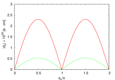
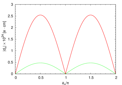
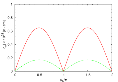
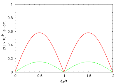
Figure 1: Gluino contribution to the neutron EDM versus $\phi_{\mu}$ (top) and $\phi_{A_{u}}=\phi_{A_{d}}$ (bottom), without (left) and with (right) QCD corrections. The solid line is the $d_{n}^{e}$ contribution, while the dotted one the corresponding $d_{n}^{c}$ contribution.

In fig. 1 we show the effect of QCD corrections on the gluino contribution to the EDM of the neutron. In the figure we plot the absolute value of $d_{n}$ as a function of $\phi_{A}$ and $\phi_{\mu}$ with the other SUSY parameters set to the values listed above.

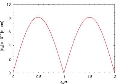
Figure 2: Chargino contribution to the neutron EDM versus $\phi_{\mu}$, without (left) and with (right) QCD corrections. We show only the $d_{n}^{e}$ contribution because the $d_{n}^{c}$ one is negligible.

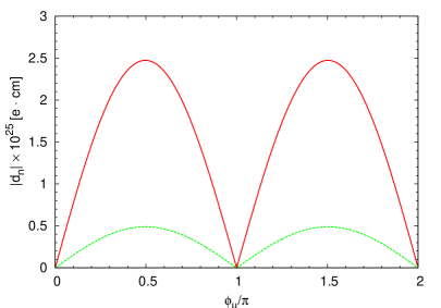
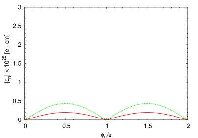
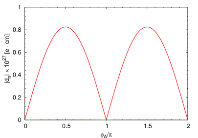
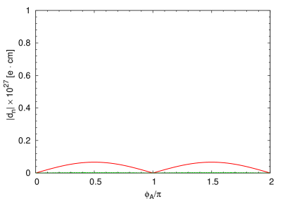
Figure 3: Neutralino contribution to the neutron EDM versus $\phi_{\mu}$ (top) and $\phi_{A_{u}}=\phi_{A_{d}}$ (bottom), without (left) or with (right) QCD corrections. The solid line is the $d_{n}^{e}$ contribution, while the dotted one the corresponding $d_{n}^{c}$ contribution.

As can be seen comparing the plots on the left, which are obtained without QCD corrections, to the ones on the right, where QCD corrections are included, the effect in this case amounts to $\sim 10\%$. Fig. 2 and fig. 3 show the corresponding analysis for chargino and neutralino contributions, respectively. Fig. 2 shows that for chargino contributions the inclusion of QCD corrections reduces the amount of CP violation generated at the $\mu_{\rm S}$ scale by a factor $\sim 50\%$. Finally, the simple analysis of the neutralino contribution discussed above is substantiated by fig. 3 where this strong reduction is clearly visible.

A popular mechanism [5] invoked to suppress the neutron EDM without resorting to extremely small phases or very heavy SUSY particles is the search for regions of the parameter space where cancellations among the three different contributions are active. It is always possible to find regions of the parameter space where contributions depending upon different parameters cancel each other, although it can be questioned if these regions can be representative of general situations. With respect to this, it is interesting to note that, since the neutralino contribution is always much more suppressed by QCD corrections than the gluino and chargino ones, the cancellation mechanism among different contributions invoked in ref. [5] should actually work between the gluino and chargino only. However, these two contributions depend upon different phase combinations. As an example, $\phi_{A}$ is only present in the gluino contribution.

2.5 Uncertainties of the LO analysis

In the above analysis all the uncertainties of the LO computation have been neglected. The uncertainties connected to the nonperturbative evaluation of the hadronic matrix elements go beyond the scope of this work, since we focus our analysis on the perturbative aspects of QCD effects. Therefore, let us assume that some nonperturbative method such as Lattice QCD will produce in the future the necessary matrix elements at a scale $\mu_{H}=2$ GeV, so that we fix the hadronic scale in our analysis. Then, we are left with the uncertainties connected to the matching between the full and the effective theory at the scale $\mu_{\rm S}$.

It is well known that in the RGE improved perturbation theory there remain unphysical $\mu_{\rm S}$-dependences which are of the order of the neglected higher order terms. Usually, this uncertainty can be estimated by varying the matching scale in a (arbitrarily chosen) given range. However, for the EDM computation, there are further sources of uncertainty. All contributions depend upon the squark masses, but the precise definition of these masses cannot be fixed at LO, so that one can use pole, $\overline{DR}$ or any other squark mass. Indeed, the difference between the results obtained using two different mass definitions is of higher order in $\alpha_{s}$ and provides an estimate of this additional LO uncertainty. Furthermore, the gluino contribution also depends on the gluino mass and, more important, on the strong coupling. Neither the definition of the gluino mass nor, in principle, the scale of $\alpha_{s}$ is fixed at LO, so that they constitute another source of uncertainty. All these uncertainties can be ameliorated only by a NLO calculation.

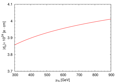
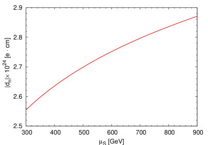
Figure 4: The $\mu_{\rm S}$ scale dependence of the chargino (left) and gluino (right) contributions to $d_{n}^{e}$ at LO.

In fig. 4 we illustrate the LO uncertainty only due to the choice of the matching point. Here and in the following NLO analysis we will use an average squark mass $m_{\tilde{q}}^{2}=(m_{\tilde{q}_{1}}^{2}+m_{\tilde{q}_{2}}^{2})/2$. In the figure we plot the LO gluino (right) and chargino (left) contributions to $|d_{n}|\simeq|d_{n}^{e}|$ as a function of the matching scale with $\alpha_{s}$ and $\overline{DR}$ masses evaluated, for simplicity, at the scale $\mu_{\rm S}$. As expected the $\mu_{\rm S}$ dependence is more pronounced in the gluino case and amounts to 10-15 % while in the chargino contribution it reaches at most 4 %.

The LO gluino contribution shows a substantial uncertainty that, including all effects, can be expected to be $\sim 20\%$. To reduce it to a level comparable to that of the chargino contribution one needs the NLO computation of this contribution that will be discussed in the next section.

3 Next-to-Leading Order Analysis

In this section we do not attempt to perform a complete NLO analysis of the QCD corrections to the neutron EDM, instead we focus on the relevant pieces needed to discuss the reduction of the scale dependence of the gluino contribution. We present the NLO anomalous dimension matrix for the electric and chromoelectric operators and the NLO Wilson coefficients for the gluino contribution. For completeness we present also the Wilson coefficients of the Weinberg operator. We recall that at the LO $C_{\scriptscriptstyle G}(\mu_{H})=0$, therefore to obtain the NLO result it is sufficient to know the LO $\gamma_{\scriptscriptstyle G},\,\gamma_{{\scriptscriptstyle G}q}$ entries of the anomalous dimension matrix.

3.1 NLO anomalous dimension

The discussion of the NLO anomalous dimension matrix is more easily accomplished in the $O_{1}^{q}$–$O_{3}$ basis of eq.(2). Indeed in this basis the anomalous dimension matrix can be organized in powers of $\alpha_{s}$ as

$$\gamma=\frac{\alpha_{s}}{4\,\pi}\gamma^{(0)}+\left(\frac{\alpha_{s}}{4\,\pi}\right)^{2}\gamma^{(1)},$$ (46)

where $\gamma^{(0)}$ is given in eq.(4) and

$$\gamma^{(1)}=\left(\begin{array}[]{ccc}\left({548\over 9}N-16\,C_{F}-{56\over 9}n_{f}\right)C_{F}&0&0\\ &&\\ \left({404\over 9}N-32\,C_{F}-{56\over 9}n_{f}\right)C_{F}&-{458\over 9}-{12\over N^{2}}+{214\over 9}N^{2}+{56\,\over 9}\frac{n_{f}}{N}-{13\over 9}N\,n_{f}&0\\ &&\\ $*$&$*$&$*$\end{array}\right).$$ (47)

We have computed the NLO anomalous dimension in eq.(47) and our results are in complete agreement with those obtained from the known NLO anomalous dimension of the $O_{7}$ and $O_{8}$ operators in the $b\to s\gamma$ process [22].

The entries in the third row are unknown but not needed at the NLO, since they contribute only to the $(i3)$ sector of the NLO magic numbers, and the initial coefficient of the Weinberg operator is vanishing at the LO. The corresponding Wilson coefficients in the $O_{e}^{q}$–$O_{G}$ basis can be easily obtained using eq.(9).

ab	43	43	54	55	63
ij	11	12	12	22	12
$W_{ij}^{ab}$	11.301	85.158	-79.353	9.9191	0
$R_{ij}^{ab}$	-8.7762	-70.209	65.693	-6.9887	0
$\delta X_{ij}^{ab}$	-0.39785	-3.1828	3.7203	-0.65874	-0.46504

Table 2: Magic numbers $R_{ij}^{ab}$ , $W_{ij}^{ab}$ and $\delta X_{ij}^{ab}$ for the NLO evolution from six to four flavours.

The simplest way to present the NLO evolution of the Wilson coefficients is via the magic numbers. Referring to the $O_{e}^{q}$–$O_{G}$ basis we can write for a generic scale $\mu$

$$\vec{\rm C}(\mu)=\vec{\rm C}^{(0)}(\mu)+\frac{\alpha_{s}(\mu)}{4\pi}\,\vec{\rm C}^{(1)}(\mu)$$ (48)

where ${\rm C}_{i}^{(0)}(\mu_{\rm S})$ is the LO Wilson coefficient at the scale $\mu_{\rm S}$ and its evolution from $\mu_{\rm S}>m_{t}$ to $\mu_{H}<m_{b}$ is given by eq.(13). The evolution of $\vec{\rm C}^{(1)}(\mu)$ from $\mu_{\rm S}>m_{t}$ to $\mu_{H}<m_{b}$ can be summarized in the following way

$${\rm C}_{i}^{(1)}(\mu_{H}) = \eta\sum_{j=1}^{3}\sum_{a=1}^{6}\sum_{b=1}^{5}\alpha_{s}(\mu_{\rm S})^{Y_{a}}\eta^{Z_{b}}g_{s}(\mu_{\rm S})^{\delta_{i1}(\delta_{j1}-1)}\left[\,X^{ab}_{ij}\,{\rm C}_{j}^{(1)}(\mu_{\rm S})\right.$$ (49)

$$\left.+\left(\delta X_{ij}^{ab}/\alpha_{s}(\mu_{\rm S})+W_{ij}^{ab}+\eta^{-1}R_{ij}^{ab}\right){\rm C}_{j}^{(0)}(\mu_{\rm S})\right].$$

The relevant entries of the NLO magic numbers $\delta X_{ij}^{ab}$ , $W_{ij}^{ab}$ and $R_{ij}^{ab}$ are given in Table 2. As expected, the evolution of $\vec{\rm C}^{(1)}(\mu_{\rm S})$ is dictated by the magic numbers derived in the LO case (see eq.(13)).

3.2 NLO Wilson coefficients

The computation of the matching conditions at the NLO level can be divided in two parts: the matching conditions for the helicity flip operators, $O^{q}_{e},\,O^{q}_{c}$, and those for the Weinberg operator $O_{\scriptscriptstyle G}$. Concerning the latter, the light quarks give a vanishing contribution so that the only relevant contribution is due the top quark that has no associated effective theory to subtract and therefore no infrared (IR) divergent terms to deal with. Instead, for helicity flip operators the computation of the NLO matching condition is, in general, a very complicated task. At the moment, even for a process like $b\to s\gamma$, that has been investigated in great detail in the last ten years, we have not yet obtained in the MSSM the complete NLO matching conditions but only partial results are available [23, 24].

We begin discussing the NLO matching conditions for $O_{e},\,O_{c}$. In the actual computation two strategies are at hand. One can match matrix elements of operators belonging to a basis, like the one in eq.(8), obtained enforcing the equation of motion, a procedure that however requires, in general, an asymptotic expansion of the relevant diagrams in the external momenta. Alternatively, one can use a larger off-shell basis and perform the matching on the off-shell matrix elements. In this case, one can use the freedom of the off-shell status to choose a suitable kinematical configuration such that the relevant Feynman diagrams can be evaluated using ordinary Taylor expansions in the external momenta. The latter strategy, applied in ref. [25] to the NLO matching conditions of the $\Delta B=1$ magnetic and chromomagnetic operators, has been employed by us in the present work following closely ref. [25] to which we refer for technical details.

The off-shell operator basis relevant for our calculation is obtained by supplementing the basis in eq.(8) with the two operators [26]

$$O_{m}^{q} = -\frac{i}{2}m_{q}\,\bar{q}\gamma_{5}q,$$

$$O_{p^{2}}^{q} = -\frac{i}{2}\bar{q}\,\not\!\!D\not\!\!D\gamma_{5}q$$ (50)

where $D_{\mu}$ is the $SU(3)\times U(1)_{Q}$ covariant derivative. The relevant terms in the Wilson coefficients are extracted via the use of the projector

$$P_{EDM}^{\mu} = \displaystyle{\frac{1}{2\,q^{6}\,(n-2)}\left\{q^{2}(n-2)(q^{2}-\not\!q\not\!p_{1}+m_{q}\not\!q)(2p_{1}-q)^{\mu}\right.}$$ (51)

$$~{}~{}~{}+\left.m_{q}^{2}\left[(n-1)(4\not\!q\not\!p_{1}(2\,p_{1}-q)^{\mu}-4\,q^{2}p_{1}^{\mu})+2\,n\,q^{2}q^{\mu}-2\,q^{2}\gamma^{\mu}\not\!q\right]\right\}\gamma_{5}$$

assuming an off-shell kinematical configuration defined by $p_{1}^{2}=p_{2}^{2}=0,~{}p_{1}\cdot q=q^{2}/2$ where $p_{1}$ and $q$ are the momentum carried by the incoming quark and the external boson, respectively, and $q^{2}\ll m_{q}^{2}$. The projector works by contracting it with the amplitudes and taking the trace, so that in eq.(51) $\mu$ is the index carried by the external boson while $n$ is the dimension of the space-time. The use of an off-shell kinematical configuration induces in the result for the “full” theory the appearance of terms that behave like $1/m_{q}^{2},\,\ln m_{q}^{2}$ as $m_{q}\to 0$. These infrared terms are eliminated by corresponding terms in the effective theory once the off-shell basis $(O_{e}^{q},\,O_{c}^{q},\,O_{m}^{q},\,O_{p^{2}}^{q})$ is employed so that the Wilson coefficients are free of infrared terms as they should.

To simplify the calculation we compute the NLO gluino contribution to the matching conditions retaining only one source of $CP$ violation, namely we keep only one power of $X_{q}$, discharging terms $X_{q}^{n}$ with $n>1$. We also work in the limit of $m_{\tilde{q}_{L}}=m_{\tilde{q}_{R}}\equiv m_{\tilde{q}}$ with $m_{\tilde{q}}$ common to all squark flavours and taking all quarks massless but the top one. Within this framework the NLO gluino corrections can be written as

$$C_{e\tilde{g}}^{q(1)}(\mu_{\rm S}) = \frac{\alpha_{s}}{4\pi\,m_{\tilde{g}}^{2}}\left\{{\rm Im}\left(\frac{X_{q}}{m_{\tilde{g}}}\right)\,\left[F_{1}\left(x_{\tilde{g}}\right)+4F_{2}\left(x_{\tilde{g}}\right)+F_{2}\left(x_{\tilde{g}},x_{t}\right)+{\rm Re}\left(\frac{m_{t}\,X_{t}}{m_{\tilde{g}}^{2}}\right)\,N_{1}\left(x_{\tilde{g}},x_{t}\right)\,\right]\right.$$ (52)

$$\left.~{}~{}+{\rm Im}\left(\frac{m_{t}\,X_{t}}{m_{\tilde{g}}^{2}}\right)\,{\rm Re}\left(\frac{X_{q}}{m_{\tilde{g}}}\right)\,N_{2}\left(x_{\tilde{g}},x_{t}\right)\,\right\},$$

$$C_{c\tilde{g}}^{q(1)}(\mu_{\rm S}) = \frac{g_{s}\,\alpha_{s}}{4\pi\,m_{\tilde{g}}^{2}}\left\{{\rm Im}\left(\frac{X_{q}}{m_{\tilde{g}}}\right)\,\left[F_{3}\left(x_{\tilde{g}}\right)+4F_{4}\left(x_{\tilde{g}}\right)+F_{4}\left(x_{\tilde{g}},x_{t}\right)+{\rm Re}\left(\frac{m_{t}\,X_{t}}{m_{\tilde{g}}^{2}}\right)\,N_{3}\left(x_{\tilde{g}},x_{t}\right)\,\right]\right.$$ (53)

$$\left.~{}~{}+{\rm Im}\left(\frac{m_{t}\,X_{t}}{m_{\tilde{g}}^{2}}\right)\,{\rm Re}\left(\frac{X_{q}}{m_{\tilde{g}}}\right)\,N_{4}\left(x_{\tilde{g}},x_{t}\right)\,\right\}$$

where in the above equations the upper line represents the $CP$ violation induced by the left-right entry in the mass matrix of the squark of type $q$ while the lower one the corresponding effect due to the stops. We have further divide the former contribution into the the part due to the quark and squark of type $q$, that of the other four squarks and massless quarks (the first two terms), and that due to the top and stops including the mixing (the last two terms). In eqs.(52-53) $x_{\tilde{g}}=m_{\tilde{g}}^{2}/m_{\tilde{q}}^{2}$, $x_{t}=m_{t}^{2}/m_{\tilde{q}}^{2}$, , where the gluino and squark masses are assumed as $\overline{DR}$ parameters, and

$$F_{i}=G_{i}+\Delta_{i}\,\ln\frac{\mu_{\rm S}^{2}}{m_{\tilde{q}}^{2}}\quad,\quad\lim_{x_{t}\rightarrow 0}F_{i}(x_{\tilde{g}},x_{t})=F_{i}(x_{\tilde{g}}).$$ (54)

The explicit expressions of the functions $G_{i}$ , $\Delta_{i}$, $N_{i}$ are reported in the Appendix. Defining

$$\tilde{\Delta}_{1} = \frac{\alpha_{s}}{4\pi\,m_{\tilde{g}}^{2}}{\rm Im}\left(\frac{X_{q}}{m_{\tilde{g}}}\right)\left(\Delta_{1}+5\Delta_{2}\right),$$

$$\tilde{\Delta}_{2} = \frac{g_{s}\,\alpha_{s}}{4\pi\,m_{\tilde{g}}^{2}}{\rm Im}\left(\frac{X_{q}}{m_{\tilde{g}}}\right)\left(\Delta_{3}+5\Delta_{4}\right)$$

we have that the coefficients of the $\ln(\mu_{\rm S}^{2}/m_{\tilde{q}}^{2})$ terms satisfy

$$\tilde{\Delta}_{i}=\frac{1}{2}\left[\left(1+i\right)\,\beta^{SUSY}_{0}+\sum_{k=\tilde{g},\tilde{q}}\gamma_{m_{k}}^{(0)}m_{k}\frac{\partial}{\partial m_{k}}+\gamma_{X_{q}}^{(0)}\right]C^{(0)}_{i}+\frac{1}{2}\sum_{j=1}^{2}\gamma_{ji}^{(0)}C^{(0)}_{j}\,,$$ (55)

with

$$\beta^{SUSY}_{0}=3\,N-n_{f}\quad,\quad\gamma_{m_{\tilde{g}}}^{(0)}=2\left(3\,N-n_{f}\right)\quad,\quad\gamma_{m_{\tilde{q}}}^{(0)}=4\,C_{F}\,m_{\tilde{g}}^{2}/m_{\tilde{q}}^{2}\quad,\quad\gamma_{X_{q}}^{(0)}=-2\,C_{F}$$

guaranteeing the cancellation of the $\mu_{\rm S}$ dependence to ${\cal O}(\alpha_{s}^{2})$ in eq.(48). We observe that the effect of the term in the square brackets in eq.(55) is to shift the coupling and the mass parameters appearing in $C^{(0)}_{i}$ from the scale $\mu_{\rm S}$ to $m_{\tilde{q}}$.

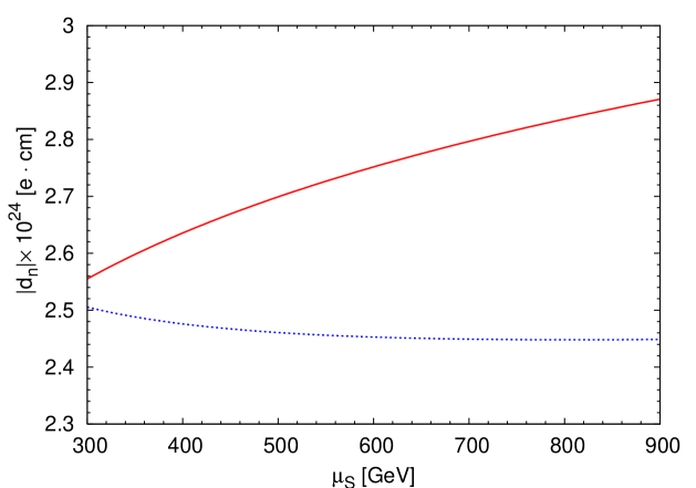
Figure 5: The $\mu_{S}$ scale dependence of the gluino contribution to $d_{n}^{e}$ at LO (upper curve) and NLO (lower curve).

As we anticipated in sec. 2.5, the inclusion of the NLO matching for the gluino contributions reduces the perturbative uncertainties down to a completely negligible level. Moreover the inclusion of NLO corrections produces a non-negligible effect. In fig. 5 we plot the scale dependence of the gluino contribution at the LO (upper line) and at the NLO (lower line) level. As shown in the figure the inclusion of the NLO contribution greatly reduces the scale dependence of the gluino contribution and lowers $|d_{n}|$ of about 10%.

Finally, for completeness, we consider also the Weinberg operator. At the scale $\mu_{\rm S}$ two-loop diagrams where top and stops together with the gluino are exchanged contribute to $C^{(1)}_{\scriptscriptstyle G}$. The relevant expressions can be gleaned from ref. [27] obtaining

$$C^{(1)}_{{\scriptscriptstyle G}\tilde{g}}(\mu_{\rm S})=\frac{g_{s}\,\alpha_{s}}{4\pi\,m_{\tilde{g}}^{2}}{\rm Im}\left(\frac{X_{t}}{m_{\tilde{g}}}\right)\,H\left(x_{\tilde{g}},x_{t}\right),$$ (56)

where the function $H$ is found in the Appendix. However, when the evolution down to a four-flavour theory is considered one has to take into account also the shift in $C^{(1)}_{{\scriptscriptstyle G}}$ induced by the $O_{c}$ operator at the $m_{b}$ threshold [13, 12, 27] or

$$C^{(1)}_{{\scriptscriptstyle G}\tilde{g}}(m_{b}^{-})=C^{(1)}_{{\scriptscriptstyle G}\tilde{g}}(m_{b}^{+})+\frac{\alpha_{s}(m_{b})}{8\,\pi}C^{b(0)}_{c\tilde{g}}(m_{b})~{},$$ (57)

where

$$C^{(1)}_{{\scriptscriptstyle G}\tilde{g}}(m_{b}^{+}) = {\eta_{b}}^{{39\over 46}}C^{(1)}_{{\scriptscriptstyle G}\tilde{g}}(\mu_{\rm S}),$$ (58)

$$C^{b(0)}_{c\tilde{g}}(m_{b}) = {\eta_{b}}^{{5\over 46}}C^{b(0)}_{c\tilde{g}}(\mu_{\rm S})$$ (59)

with $\eta_{b}=\alpha_{s}(\mu_{\rm S})/\alpha_{s}(m_{b})$.

4 Conclusions

In this paper we have discussed the LO and NLO QCD corrections to the electric dipole moment of the neutron in the MSSM. We pointed out the importance of the mixing between the electric and chromoelectric operators that was always neglected in previous analyses. Also we noticed that the QCD renormalization factor of the dipole operator in absence of mixing should be less than 1 while its widely used estimate is $\eta^{ED}=1.53$ [15].

In the MSSM the prediction for the EDM can easily clash with the experimental upper bound $|d_{n}|<6.310^{-26}$ e$\cdot$cm [28] if the phases in the mass parameters are arbitrarily chosen. To avoid conflict with the experimental bound one can consider models with approximate CP symmetries [29] or flavour off diagonal phases [30] where small phases can be naturally obtained. Another possibility is represented by a cancellation mechanism among different contributions to the quark EDM which could allow O$(1)$ phases. However we noticed that, because of the mixing between the electric and chromoelectric operators, the neutralino contribution is always much more suppressed than the gluino and chargino ones so that the cancellation mechanism should actually mainly work between the latter contributions that, however, depend upon phases connected with apparently unrelated terms in the MSSM Lagrangian.

Our results show that the NLO corrections we considered lower the prediction of the EDM of about 10% with respect to LO. Moreover the dependence on the matching scale is drastically reduced. Clearly, a complete NLO analysis will require, besides the gluino contribution we focused on, the other two contributions, in particular the chargino one.

We have mainly focused on the perturbative aspects of the problem but, in order to achieve a complete analysis of the SUSY constraints from the neutron EDM, a lattice computation of the relevant matrix elements is mandatory.

Finally we notice that our analytic formulae for the magic numbers can also be used for the evolutions of the Wilson coefficients in any extension of the SM with new heavy particles, unless large four fermion operators are generated at the matching scale. This happens, for example, in supersymmetric models with large $\tan\beta$ [31].

5 Acknowledgments

We thank A. Isidori for collaborating with us in the early stage of this project. This work was supported in part by the EU network ”The quest for unification” under the contract MRTN-CT-2004-503369.

Appendix

In this appendix we give the explicit expressions of the one- and two-loop functions that appear in the Wilson coefficients.

The explicit expressions of the one-loop functions entering in eqs. (24-34) are given by

$$\tilde{A}\left(x_{1},x_{2}\right) = -\frac{x_{1}x_{2}\left(x_{1}x_{2}+x_{1}+x_{2}-3\right)}{2\left(x_{1}-1\right)^{2}\left(x_{2}-1\right)^{2}}-\frac{x_{1}x_{2}}{\left(x_{1}-x_{2}\right)}\left[\frac{x_{1}\ln\,x_{1}}{\left(x_{1}-1\right)^{3}}-\frac{x_{2}\,\ln\,x_{2}}{\left(x_{2}-1\right)^{3}}\right]$$

$$\tilde{B}\left(x_{1},x_{2}\right) = \frac{x_{1}x_{2}\left(3x_{1}x_{2}-x_{1}-x_{2}-1\right)}{2\left(x_{1}-1\right)^{2}\left(x_{2}-1\right)^{2}}+\frac{x_{1}x_{2}}{\left(x_{1}-x_{2}\right)}\left[\frac{x_{1}^{2}\ln\,x_{1}}{\left(x_{1}-1\right)^{3}}-\frac{x_{2}^{2}\,\ln\,x_{2}}{\left(x_{2}-1\right)^{3}}\right]$$

$$\tilde{C}\left(x_{1},x_{2}\right) = \frac{x_{1}x_{2}\left(3x_{1}x_{2}+5x_{1}+5x_{2}-13\right)}{3\left(x_{1}-1\right)^{2}\left(x_{2}-1\right)^{2}}$$

$$-\frac{x_{1}x_{2}}{3\left(x_{1}-x_{2}\right)}\left[\frac{x_{1}\left(x_{1}-9\right)\ln\,x_{1}}{\left(x_{1}-1\right)^{3}}-\frac{x_{2}\left(x_{2}-9\right)\,\ln\,x_{2}}{\left(x_{2}-1\right)^{3}}\right]$$

$$A\left(x\right) = \frac{x\left(x-3\right)}{2\left(x-1\right)^{2}}+\frac{x\,\ln x}{\left(x-1\right)^{3}}$$

$$B\left(x\right) = \frac{x\left(x+1\right)}{2\left(x-1\right)^{2}}-\frac{x^{2}\,\ln x}{\left(x-1\right)^{3}}~{}.$$ (A1)

In the case of equal masses the functions $\tilde{A},\,\tilde{B},\,\tilde{C}$ reduce to

$$\tilde{A}\left(x\right) = -\frac{x^{2}\,\left(x+5\right)}{2\,\left(x-1\right)^{3}}+\frac{x^{2}\,\left(2x+1\right)\,\ln x}{\left(x-1\right)^{4}}$$

$$\tilde{B}\left(x\right) = \frac{x^{2}\,\left(5x+1\right)}{2\,\left(x-1\right)^{3}}-\frac{x^{3}\,\left(x+2\right)\,\ln x}{\left(x-1\right)^{4}}$$

$$\tilde{C}\left(x\right) = \frac{2\,x^{2}\,\left(x+11\right)}{3\,\left(x-1\right)^{3}}+\frac{x^{2}\,\left(x^{2}-16x-9\right)\,\ln x}{3\left(x-1\right)^{4}}~{}.$$ (A2)

We list now the two-loop functions that appear in eqs. (52-53). To simplify the expressions, we perform an expansion in the top mass reporting only the first term in $x_{t}$. In particular, recalling eq. (54), we write

$$F_{2}\left(x_{\tilde{g}},x_{t}\right) = G_{2}\left(x_{\tilde{g}},x_{t}\right)+\Delta_{2}\left(x_{\tilde{g}}\right)\,\ln\frac{\mu_{\rm S}^{2}}{m_{\tilde{q}}^{2}}$$

$$\simeq G_{2}\left(x_{\tilde{g}}\right)+x_{t}\,G_{2}^{t}\left(x_{\tilde{g}}\right)+\Delta_{2}\left(x_{\tilde{g}}\right)\,\ln\frac{\mu_{\rm S}^{2}}{m_{\tilde{q}}^{2}}$$

$$F_{4}\left(x_{\tilde{g}},x_{t}\right) = G_{4}\left(x_{\tilde{g}},x_{t}\right)+\Delta_{4}\left(x_{\tilde{g}}\right)\,\ln\frac{\mu_{\rm S}^{2}}{m_{\tilde{q}}^{2}}$$

$$\simeq G_{4}\left(x_{\tilde{g}}\right)+x_{t}\,G_{4}^{t}\left(x_{\tilde{g}}\right)+x_{t}\ln x_{t}\,S_{4}\left(x_{\tilde{g}}\right)+\Delta_{4}\left(x_{\tilde{g}}\right)\,\ln\frac{\mu_{\rm S}^{2}}{m_{\tilde{q}}^{2}}$$

$$N_{i}\left(x_{\tilde{g}},x_{t}\right) \simeq \sqrt{x_{t}}\,N_{i}^{t}\left(x_{\tilde{g}}\right)+\sqrt{x_{t}}\ln x_{t}\,R_{i}^{t}\left(x_{\tilde{g}}\right)~{}.$$

We find

$$G_{1}\left(x\right) = \frac{8x^{2}\left(51x^{3}+413x^{2}-1473x-251\right)}{27\left(x-1\right)^{4}}-\frac{16\left(8x^{2}+293x-13\right)}{27\left(x-1\right)^{4}}\,{\rm Li}_{2}\left(1-x\right)$$ (A3)

$$~{}+\frac{8x^{2}\left(127x^{4}-1075x^{3}+480x^{2}+405x+27\right)\,\ln^{2}x}{27\left(x-1\right)^{6}}$$

$$~{}-\frac{8x^{2}\left(48x^{4}+228x^{3}-1105x^{2}-548x+81\right)\,\ln x}{27\left(x-1\right)^{5}}$$

$$G_{2}\left(x\right) = \frac{64x^{2}\left(x^{2}+4x-2\right)}{3\left(x-1\right)^{4}}-\frac{16x^{2}\left(x+5\right)}{3\left(x-1\right)^{3}}\,{\rm Li}_{2}\left(1-x\right)-\frac{16x^{3}\left(x^{2}+4x-1\right)\ln x}{\left(x-1\right)^{5}}$$ (A4)

$$G_{3}\left(x\right) = -\frac{x^{2}\left(129x^{3}-2903x^{2}+1083x+21851\right)}{54\left(x-1\right)^{4}}-\frac{4\left(113x^{2}+281x+110\right)}{27\left(x-1\right)^{4}}\,{\rm Li}_{2}\left(1-x\right)$$ (A5)

$$~{}+\frac{x^{2}\left(539x^{4}-2282x^{3}-6744x^{2}+7578x+621\right)\,\ln^{2}x}{27\left(x-1\right)^{6}}$$

$$~{}+\frac{x^{2}\left(96x^{4}-5019x^{3}+13357x^{2}+10583x+1719\right)\,\ln x}{54\left(x-1\right)^{5}}$$

$$G_{4}\left(x\right) = -\frac{x^{2}\left(17x^{2}-310x+101\right)}{3\left(x-1\right)^{4}}+\frac{2x^{2}\left(x-40\right)}{3\left(x-1\right)^{3}}\,{\rm Li}_{2}\left(1-x\right)+\frac{x^{2}\left(2x^{3}-67x^{2}+4x-3\right)\ln x}{\left(x-1\right)^{5}}$$

$$G_{2}^{t}\left(x\right) = \frac{8x^{2}\left(x^{2}+76x+175\right)}{9\left(x-1\right)^{4}}+\frac{32x^{2}\left(x+3\right)}{\left(x-1\right)^{5}}\,{\rm Li}_{2}\left(1-x\right)-\frac{32x^{3}\left(2x+7\right)\ln x}{3\left(x-1\right)^{5}}$$ (A6)

$$G_{4}^{t}\left(x\right) = -\frac{x^{2}\left(17x^{2}+230x-4387\right)}{18\left(x-1\right)^{4}}+\frac{2x^{2}\left(3x^{2}-8x+81\right)}{\left(x-1\right)^{5}}\,{\rm Li}_{2}\left(1-x\right)$$ (A7)

$$~{}+\frac{x^{2}\left(53x^{2}-305x+18\right)\ln x}{3\left(x-1\right)^{5}}\ln x$$

$$S_{4}\left(x\right) = -\frac{x^{2}\left(x^{2}+10x+1\right)}{\left(x-1\right)^{4}}+\frac{6x^{3}\left(x+1\right)\ln x}{\left(x-1\right)^{5}}$$ (A8)

$$N_{1}^{t}\left(x\right) = -\frac{4x^{\frac{5}{2}}\left(x^{3}+8x^{2}+173x+34\right)}{9\left(x-1\right)^{4}}-\frac{32x^{\frac{7}{2}}\left(x+2\right)\ln x}{3\left(x-1\right)^{5}}$$ (A9)

$$~{}-\frac{16x^{\frac{5}{2}}\left(5x^{2}+17x+2\right)}{3\left(x-1\right)^{5}}{\rm Li}_{2}\left(1-x\right)$$

$$N_{2}^{t}\left(x\right) = -\frac{4x^{\frac{5}{2}}\left(x^{2}+x+34\right)}{9\left(x-1\right)^{3}}-\frac{16x^{\frac{5}{2}}\left(x+2\right)}{3\left(x-1\right)^{4}}{\rm Li}_{2}\left(1-x\right)$$ (A10)

$$N_{3}^{t}\left(x\right) = -\frac{x^{\frac{5}{2}}\left(11x^{3}-158x^{2}+1225x+542\right)}{18\left(x-1\right)^{4}}+\frac{2x^{\frac{5}{2}}\left(2x^{2}-86x-9\right)\ln x}{3\left(x-1\right)^{5}}$$ (A11)

$$~{}+\frac{2x^{\frac{5}{2}}\left(5x^{2}-181x-52\right)}{3\left(x-1\right)^{5}}{\rm Li}_{2}\left(1-x\right)$$

$$N_{4}^{t}\left(x\right) = -\frac{x^{\frac{5}{2}}\left(11x^{3}-114x^{2}+753x-758\right)}{18\left(x-1\right)^{4}}-\frac{6x^{\frac{5}{2}}\left(6x-1\right)\ln x}{\left(x-1\right)^{5}}$$ (A12)

$$~{}+\frac{2x^{\frac{5}{2}}\left(x^{2}-89x+52\right)}{3\left(x-1\right)^{5}}{\rm Li}_{2}\left(1-x\right)$$

$$R_{3}^{t}\left(x\right) = -\frac{x^{\frac{7}{2}}\left(x^{2}-8x-17\right)}{2\left(x-1\right)^{4}}-\frac{3x^{\frac{7}{2}}\left(3x+1\right)\ln x}{\left(x-1\right)^{5}}$$ (A13)

$$R_{4}^{t}\left(x\right) = -\frac{x^{\frac{7}{2}}\left(x^{2}-8x-17\right)}{2\left(x-1\right)^{4}}-\frac{3x^{\frac{7}{2}}\left(3x+1\right)\ln x}{\left(x-1\right)^{5}}$$ (A14)

$$\Delta_{1}\left(x\right) = \frac{16x^{2}\left(8x^{3}+13x^{2}-176x-37\right)}{9\left(x-1\right)^{4}}-\frac{16x^{2}\left(29x^{3}-97x^{2}-115x-9\right)\ln x}{9\left(x-1\right)^{5}}$$ (A15)

$$\Delta_{2}\left(x\right) = \frac{8x^{2}\left(7x^{2}+16x+1\right)}{3\left(x-1\right)^{4}}-\frac{16x^{3}\left(x^{2}+7x+4\right)\ln x}{3\left(x-1\right)^{5}}$$ (A16)

$$\Delta_{3}\left(x\right) = -\frac{8x^{2}\left(2x^{3}-83x^{2}+268x+197\right)}{9\left(x-1\right)^{4}}-\frac{4x^{2}\left(59x^{3}-67x^{2}-643x-117\right)\ln x}{9\left(x-1\right)^{5}}$$ (A17)

$$\Delta_{4}\left(x\right) = \frac{2x^{2}\left(x^{2}+64x+31\right)}{3\left(x-1\right)^{4}}+\frac{2x^{2}\left(x^{3}-29x^{2}-59x-9\right)\ln x}{3\left(x-1\right)^{5}}$$ (A18)

where ${\rm Li}_{2}(z)=-\int_{0}^{z}{\rm d}t\left[\ln(1-t)/t\right]$ is the dilogarithm function.

We observe that we have to take care of the fact that the naive dimensional regularization (NDR) we used violate supersymmetry, because the gauge boson and gaugino interactions with matter are different at one loop. Supersymmetric Ward identity can be restored with an appropriate shift in the gluino-squark-quark coupling and with a shift of the gluino mass [23, 32]. Explicitly, the coupling and the gluino mass in the lowest order formula (eqs. (25,26)), must be replaced with

$$g_{s} \rightarrow g_{s}(1+\frac{\alpha_{s}}{4\pi}\frac{4}{3})$$ (A19)

$$m_{\tilde{g}} \rightarrow m_{\tilde{g}}(1+\frac{\alpha_{s}}{4\pi}3)~{}.$$ (A20)

Finally, the function $H$ entering in the Weinberg operator (eq. (56)) is given by

$$H\left(x_{\tilde{g}},x_{t}\right) \simeq H\left(x_{\tilde{g}}\right)+x_{t}\,H_{1}^{t}\left(x_{\tilde{g}}\right)+x_{t}\ln x_{t}\,H_{2}^{t}\left(x_{\tilde{g}}\right)$$

$$H\left(x\right) = \frac{x^{2}\left(x+11\right)}{3\left(x-1\right)^{3}}+\frac{x^{2}\left(x^{2}-16x-9\right)\ln x}{6\left(x-1\right)^{4}}$$

$$H_{1}^{t}\left(x\right) = \frac{x\left(5x^{3}+265x^{2}+455x+27\right)}{6\left(x-1\right)^{5}}+\frac{2x^{2}\left(4x^{3}-93x^{2}-258x-81\right)\ln x}{3\left(x-1\right)^{6}}$$

$$~{}+\frac{2x^{2}\left(x^{3}-12x^{2}-51x-18\right)}{\left(x-1\right)^{6}}{\rm Li}_{2}\left(1-x\right)$$

$$H_{2}^{t}\left(x\right) = -\frac{x\left(11x^{3}-223x^{2}-259x-9\right)}{6\left(x-1\right)^{5}}+\frac{x^{2}\left(x^{3}-12x^{2}-51x-18\right)\ln x}{\left(x-1\right)^{6}}~{}~{}.$$ (A21)

References

• [1] C. Balazs, M. Carena, A. Menon, D. E. Morrissey and C. E. M. Wagner, Phys. Rev. D 71 (2005) 075002 [arXiv:hep-ph/0412264].
• [2] M. Bona et al. [UTfit Collaboration], [arXiv:hep-ph/0509219].
• [3] F. Gabbiani, E. Gabrielli, A. Masiero and L. Silvestrini, Nucl. Phys. B 477 (1996) 321 [arXiv:hep-ph/9604387].
• [4] A. Bartl, T. Gajdosik, E. Lunghi, A. Masiero, W. Porod, H. Stremnitzer and O. Vives, [arXiv:hep-ph/0112179].
• [5] T. Ibrahim and P. Nath, Phys. Rev. D 58 (1998) 111301 [Erratum-ibid. D 60 (1999) 099902] [arXiv:hep-ph/9807501]; Phys. Rev. D 57 (1998) 478 [Erratum-ibid. D 58 (1998) 019901, Erratum-ibid. D 60 (1999) 079903, Erratum-ibid. D 60 (1999) 119901] [arXiv:hep-ph/9708456].
• [6] S. Pokorski, J. Rosiek and C. A. Savoy, Nucl. Phys. B 570 (2000) 81 [arXiv:hep-ph/9906206].
• [7] D. Chang, W. Y. Keung and A. Pilaftsis, Phys. Rev. Lett.  82 (1999) 900 [Erratum-ibid.  83 (1999) 3972] [arXiv:hep-ph/9811202]; S. Abel, S. Khalil and O. Lebedev, Nucl. Phys. B 606 (2001) 151 [arXiv:hep-ph/0103320]; T. F. Feng, X. Q. Li, J. Maalampi and X. m. Zhang, Phys. Rev. D 71 (2005) 056005 [arXiv:hep-ph/0412147].
• [8] M. Ciuchini, E. Franco, V. Lubicz, G. Martinelli, I. Scimemi and L. Silvestrini, Nucl. Phys. B 523 (1998) 501 [arXiv:hep-ph/9711402]; M. Ciuchini et al., JHEP 9810 (1998) 008 [arXiv:hep-ph/9808328]; A. J. Buras, M. Misiak and J. Urban, Nucl. Phys. B 586 (2000) 397 [arXiv:hep-ph/0005183]; D. Becirevic et al., Nucl. Phys. B 634 (2002) 105 [arXiv:hep-ph/0112303]; M. Ciuchini, E. Franco, A. Masiero and L. Silvestrini, Phys. Rev. D 67 (2003) 075016 [Erratum-ibid. D 68 (2003) 079901] [arXiv:hep-ph/0212397].
• [9] C. R. Allton et al., Phys. Lett. B 453 (1999) 30 [arXiv:hep-lat/9806016]; D. Becirevic, V. Gimenez, G. Martinelli, M. Papinutto and J. Reyes, JHEP 0204 (2002) 025 [arXiv:hep-lat/0110091]; D. Becirevic and G. Villadoro, Phys. Rev. D 70 (2004) 094036 [arXiv:hep-lat/0408029].
• [10] M. Ciuchini, E. Franco, L. Reina and L. Silvestrini, Nucl. Phys. B 421 (1994) 41 [arXiv:hep-ph/9311357].
• [11] S. Weinberg, Phys. Rev. Lett.  63 (1989) 2333.
• [12] E. Braaten, C. S. Li and T. C. Yuan, Phys. Rev. Lett.  64 (1990) 1709; Phys. Rev. D 42 (1990) 276.
• [13] G. Boyd, A. K. Gupta, S. P. Trivedi and M. B. Wise, Phys. Lett. B 241 (1990) 584.
• [14] M. Dine and W. Fischler, Phys. Lett. B 242, 239 (1990).
• [15] R. Arnowitt, J. L. Lopez and D. V. Nanopoulos, Phys. Rev. D 42 (1990) 2423.
• [16] E. Shintani et al., [arXiv:hep-lat/0509123]; E. Shintani et al., Phys. Rev. D 72 (2005) 014504 [arXiv:hep-lat/0505022].
• [17] M. Pospelov and A. Ritz, Phys. Rev. D 63 (2001) 073015 [arXiv:hep-ph/0010037]; D. A. Demir, M. Pospelov and A. Ritz, Phys. Rev. D 67 (2003) 015007 [arXiv:hep-ph/0208257].
• [18] A. Pich and E. de Rafael, Nucl. Phys. B 367 (1991) 313; J. Hisano and Y. Shimizu, Phys. Rev. D 70 (2004) 093001 [arXiv:hep-ph/0406091].
• [19] A. Manohar and H. Georgi, Nucl. Phys. B 234 (1984) 189.
• [20] B. C. Allanach et al., in Proc. of the APS/DPF/DPB Summer Study on the Future of Particle Physics (Snowmass 2001) ed. N. Graf, Eur. Phys. J. C 25 (2002) 113 [eConf C010630 (2001) P125] [arXiv:hep-ph/0202233]; P. Skands et al., JHEP 0407 (2004) 036 [arXiv:hep-ph/0311123]; B. C. Allanach et al. [Beyond the Standard Model Working Group Collaboration], [arXiv:hep-ph/0402295].
• [21] B. C. Allanach, S. Kraml and W. Porod, JHEP 0303 (2003) 016 [arXiv:hep-ph/0302102]; G. Belanger, S. Kraml and A. Pukhov, [arXiv:hep-ph/0502079].
• [22] M. Misiak and M. Munz, Phys. Lett. B 344 (1995) 308 [arXiv:hep-ph/9409454].
• [23] M. Ciuchini, G. Degrassi, P. Gambino and G. F. Giudice, Nucl. Phys. B 534 (1998) 3 [arXiv:hep-ph/9806308].
• [24] C. Bobeth, M. Misiak and J. Urban, Nucl. Phys. B 567 (2000) 153 [arXiv:hep-ph/9904413]; G. Degrassi, P. Gambino and G. F. Giudice, JHEP 0012 (2000) 009 [arXiv:hep-ph/0009337]; F. Borzumati, C. Greub and Y. Yamada, Phys. Rev. D 69 (2004) 055005 [arXiv:hep-ph/0311151].
• [25] M. Ciuchini, G. Degrassi, P. Gambino and G. F. Giudice, Nucl. Phys. B 527, 21 (1998) [arXiv:hep-ph/9710335].
• [26] H. Simma, Z. Phys. C 61 (1994) 67 [arXiv:hep-ph/9307274].
• [27] J. Dai, H. Dykstra, R. G. Leigh, S. Paban and D. Dicus, Phys. Lett. B 237 (1990) 216 [Erratum-ibid. B 242 (1990) 547].
• [28] P. G. Harris et al., Phys. Rev. Lett.  82 (1999) 904.
• [29] M. Dine, E. Kramer, Y. Nir and Y. Shadmi, Phys. Rev. D 63 (2001) 116005 [arXiv:hep-ph/0101092].
• [30] S. Abel, D. Bailin, S. Khalil and O. Lebedev, Phys. Lett. B 504 (2001) 241 [arXiv:hep-ph/0012145].
• [31] S. M. Barr, Phys. Rev. Lett.  68 (1992) 1822; O. Lebedev and M. Pospelov, Phys. Rev. Lett.  89 (2002) 101801 [arXiv:hep-ph/0204359]; A. Pilaftsis, Nucl. Phys. B 644 (2002) 263 [arXiv:hep-ph/0207277].
• [32] S. P. Martin and M. T. Vaughn, Phys. Lett. B 318 (1993) 331 [arXiv:hep-ph/9308222].