Effects of LatticeQCD EoS and Continuous Emission on Some Observables

Abstract

Effects of lattice-QCD-inspired equations of state and continuous emission on some observables are discussed, by solving a 3D hydrodynamics. The particle multiplicity as well as $v_{2}$ are found to increase in the mid-rapidity. We also discuss the effects of the initial-condition fluctuations.

1 HYDRODYNAMIC MODELS

Hydrodynamics is one of the main tools for studying the collective flow in high-energy nuclear collisions. Here, we shall examine some of the main ingredients of such a description and see how likely more realistic treatment of these elements may affect some of the observable quantities. The main components of any hydrodynamic model are the initial conditions, the equations of motion, equations of state and some decoupling prescription. We shall discuss how these elements are chosen in our studies.

Initial Conditions: In usual hydrodynamic approach, one assumes some highly symmetric and smooth initial conditions (IC). However, since our systems are small, large event-by-event fluctuations are expected in real collisions, so this effect should be taken into account. We introduce such IC fluctuations by using an event simulator. As an example, we show here the energy density for central Au+Au collisions at 130A GeV,

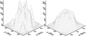
Figure 1: The initial energy density at $\eta=0$ is plotted in units of GeV/fm³. One random event is shown vs. average over 30 random events ($\simeq$ smooth initial conditions in the usual hydro approach).

given by NeXuS nexus . Some consequences of such fluctuations have been discussed elsewherefluctuations ; hbt-prl ; review . We shall discuss some others in Sec.2.

Equations of Motion: In hydrodynamics, the flow is governed by the continuity equations expressing the conservation of energy-momentum, baryon-number and other conserved charges. Here, for simplicity, we shall consider only the energy-momentum and the baryon number. Since our systems have no symmetry as discussed above, we developed a special numerical code called SPheRIO (Smoothed Particle hydrodynamic evolution of Relativistic heavy IOn collisions) spherio , based on the so called Smoothed-Paricle Hydrodynamics (SPH) algorithm sph . The main characteristic of SPH is the parametrization of the flow in terms of discrete Lagrangian coordinates attached to small volumes (called “particles”) with some conserved quantities.

Equations of State: In high-energy collisions, one often uses equations of state (EoS) with a first-order phase transition, connecting a high-temperature QGP phase with a low-temperature hadron phase. A detailed account of such EoS may be found, for instance, in review . We shall denote them 1OPT EoS. However, lattice QCD showed that the transition line has a critical end point and for small net baryon surplus the transition is of crossover type LQCD . The following parametrization may reproduce this behavior, in practice:

$$P = \lambda P_{H}+(1-\lambda)P_{Q}+2\delta/{\sqrt{(P_{Q}-P_{H})^{2}+4\delta}}\ ,$$ (1)

$$s = \lambda s_{H}+(1-\lambda)s_{Q}\,,$$ (2)

$$\epsilon = \lambda\epsilon_{H}+(1-\lambda)\epsilon_{Q}-{2\,\left[1+(\mu/\mu_{c})^{2}\right]\,\delta}/{\sqrt{(P_{Q}-P_{H})^{2}+4\delta}}\ ,$$ (3)

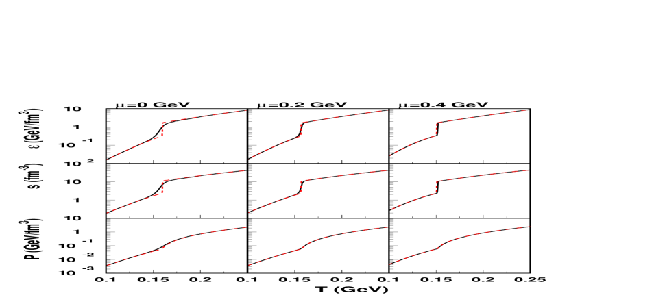
Figure 2: A comparison of $\varepsilon(T)$, $s(T)$ and $P(T)$ as given by our parametrization with a critical point (solid lines) and those with a first-order phase transition (dashed lines).

where $\lambda\equiv[1-(P_{Q}-P_{H})/\sqrt{(P_{Q}-P_{H})^{2}+4\delta}\ ]/2$ and suffixes $Q$ and $H$ denote those quantities given by the MIT bag model and the hadronic resonance gas, respectively, and $\delta\equiv\delta(\mu_{b})=\delta_{0}\exp[-(\mu_{b}/\mu_{c})^{2}]$, with $\mu_{c}=$const. As is seen, when $\delta(\mu_{b})\not=0$, the transition from hadron phase to QGP is smooth. We could choose $\delta(\mu_{b})$ so to make it exactly 0 when $\mu_{b}>\mu_{c}\,$, to guarantee the first-order phase transition there. However, in practice our choice above showed to be enough. We shall denote the EoS given above, with $\delta_{0}\not=0$, CP EoS. Let us compare, in Figure 2, $\varepsilon(T)$, $s(T)$ and $P(T)$, given by the two sets of EoS. one can see that the crossover behavior is correctly reproduced by our parametrization for CP EoS, while finite jumps in $\varepsilon$ and $s$ are exhibited by 1OPT EoS, at the transition temperature. It is also seen, as mentioned above, that at $\mu_{b}\sim 0.4\,$GeV the two EoS are indistinguishable. Now, since in a real collision what is directly given is the energy distribution at a certain initial time (besides $n_{b}$, $s$, etc.), whereas $T$ is defined with the use of the former, we plotted some quantities as function of $\varepsilon$ in Figure 3. One immediately sees there some remarkable differences between the two sets of EoS: naturally $p$ is not constant for CP EoS in the crossover region; moreover, $s$ is larger. We will see in Sec.2 that these features affect the observables in non-negligible way.

Decoupling Prescription: Usually, one assumes decoupling on a sharply defined hypersurface. We call this Sudden Freeze Out (FO). However, since our systems are small, particles may escape from a layer with thickness comparable with the systems’ sizes. We proposed an alternative description called Continuous Emission (CE) ce which, as compared to FO, we believe closer to what happens in the actual collisions. In CE, particles escape from any space-time point $x^{\mu}$, according to a momentum-dependent

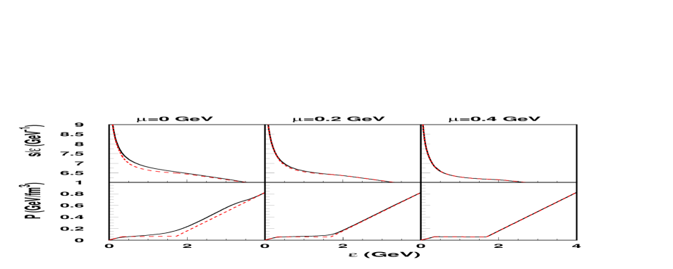
Figure 3: Plots of $s/\varepsilon$ and $P$ as function of $\varepsilon$ for the two EoS shown in Figure 2.

escaping probability ${\cal P}(x,k)=\exp\left[-\int_{\tau}^{\infty}\rho(x^{\prime})\,\sigma v\;\mathrm{d}\tau^{\prime}\right].$ To implement CE in SPheRIO code, we had to approximate it to make the computation practicable. We took ${\cal P}$ on the average, i.e.,

$${\cal P}(x,k)\rightarrow\langle{\cal P}(x,k)\rangle\equiv{\cal P}(x)=\exp\left(-\kappa\ s^{2}/|\mathrm{d}s/\mathrm{d}\tau|\right).$$ (4)

The last equality has been obtained by making a linear approximation of the density $\rho(x^{\prime})=\alpha\,s(x^{\prime})$ and $\kappa=0.5\,\alpha\,\langle\sigma v\rangle$ is estimated to be 0.3 , corresponding to $\langle\sigma v\rangle\approx$ 2 fm². It will be shown in Sec. 2 that CE gives important changes in some observables.

2 RESULTS

Let us now show results of computation of some observables, as described above, for Au+Au at 200A GeV. We start computing $\eta$ and $p_{T}$ distributions for charged particles, to fix the parameters. Then, $v_{2}$ and HBT radii are computed free of parameters.

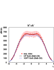
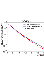
Figure 4: $\eta$ and $p_{T}$ distributions for the most central Au+Au at 200A GeV. Results of CP EoS and 1OPT EoS are compared. The data are from PHOBOS Collab.phobos1 .

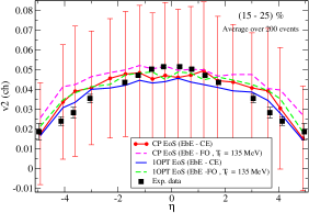
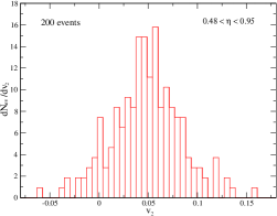
Figure 5: Left: $\eta$ distribution of $v_{2}$ for charged particles in the centrality $(15-25)$% Au+Au at 200A GeV, computed with fluctuating IC. The vertical bars indicate dispersions. The data are from PHOBOS Collab.phobos3 . Right: $v_{2}$ distribution in the interval $0.48<\eta<0.95\,$, corresponding to CP EoS and CE.

Pseudo-rapidity distribution: Figure 3 shows that the inclusion of a critical end point increases the entropy per energy. This means that, given the same total energy, CP EoS produces larger multiplicity, which is clearly shown in the left panel of Figure 4, especially in the mid-rapidity region. Now, we shall mention that, once the equations of state are chosen, fluctuating IC produce smaller multiplicity, for the same decoupling prescription, as compared with the case of smooth averaged IC review .

Transverse-Momentum Distribution: As discussed in Sec. 1, since the pressure does not remain constant in the crossover region, we expect that the transverse acceleration is larger for CP EoS, as compared with 1OPT EoS case. In effect, the right panel of Figure 4 does show that $p_{T}$ distribution is flatter for CP EoS, but the difference is small. The freezeout temperature suggested by $\eta$ and $p_{T}$ distributions turned out to be $T_{f}\simeq 135-140\,$MeV.

Elliptic-Flow Parameter $v_{2}$: We show, in Figure 5, results for the $\eta$ distribution of $v_{2}$ for Au+Au collisions at 200A GeV. As seen, CP EoS gives larger $v_{2}\,$, as a consequence of larger acceleration in this case as discussed in Sec.1. Notice that CE makes the curves narrower, as a consequence of earlier emission of particles, so with smaller acceleration, at large-$|\eta|$ regions. Due to the IC fluctuations, the resulting fluctuations of $v_{2}$ are large, as seen in Figures 5. It would be nice to measure such a $v_{2}$ distribution, which would discriminate among several microscopic models for the initial stage of nuclear collisions.

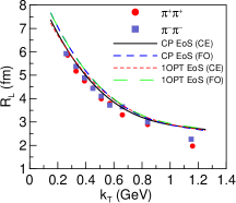
Figure 6: $k_{T}$ dependence of HBT radius $R_{L}$ for $\pi$ in the most central Au+Au at 200A GeV, computed with fluctuating IC. The data are from PHENIX Collab.phenix .

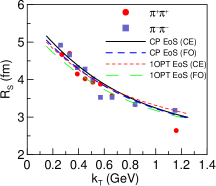
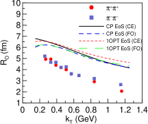
Figure 7: $k_{T}$ dependence of HBT radii $R_{s}$ and $R_{o}$ for pions in the most central Au+Au at 200A GeV, computed with event-by-event fluctuating IC. The data are from PHENIX Collab.phenix .

HBT Radii: Here, we show our results for the HBT radii, in Gaussian approximation as often used, for the most central Au+Au collisions at 200A GeV. As seen in Figures 6 and 7, the differences between CP EoS results and those for 1OPT EoS are small. For $R_{s}\,$, and especially for $R_{o}\,$, one sees that CP EoS combined with continuous emission gives steeper $k_{T}$ dependence, closer to the data. However, there is still numerical discrepancy in this case.

3 CONCLUSIONS AND OUTLOOKS

In this work, we introduced a parametrization of lattice-QCD EoS, with a first-order phase transition at large $\mu_{b}$ and a crossover behavior at smaller $\mu_{b}\,$. By solving the hydrodynamic equations, we studied the effects of such EoS and the continuous emission. Some conclusions are: i) The multiplicity increases for these EoS in the mid-rapidity; ii) The $p_{T}$ distribution becomes flatter, although the difference is small; iii) $v_{2}\,$ increases; CE makes the $\eta$ distribution narrower; iv) HBT radii slightly closer to data.

In our calculations, the effect of the continuous emission on the interacting component has not been taken into account. A more realistic treatment of this effect probably makes $R_{o}$ smaller, since the duration for particle emission becomes smaller in this case. Another improvement we should make is the approximations we used for ${\cal P}(x,p)$.

References

- (1) H.J. Drescher, F.M. Liu, S. Ostapchenko, T. Pierog and K. Werner, Phys. Rev. C 65, 054902 (2002).
- (2) M. Gyulassy, D.H. Rischke and B. Zhang, Nucl. Phys. A 613, 397–434 (1997).
- (3) B.R. Schlei and D. Strotman, Phys. Rev. C 59, 9–12 (1999).
- (4) S. Daté, K. Kumagai, O. Miyamura, H. Sumiyoshi and Xiao-Ze Zhang, J. Phys. Soc. Japan 64, 766–776 (1995).
- (5) Y. Hama, F. Grassi, O. Socolowski Jr., C.E. Aguiar, T. Kodama, L.L.S. Portugal, B.M. Tavares and T. Osada, in Proc. of 32nd. ISMD, eds. A. Sissakian et al. (World Sci. – Singapore, 2003) pp.65–68.
- (6) O. Socolowski Jr., F. Grassi, Y. Hama and T. Kodama, Phys. Rev. Lett. 93, 182301 (2004).
- (7) Y. Hama, T. Kodama and O. Socolowski Jr., Braz. J. Phys. 35, 24–51 (2005).
- (8) C.E. Aguiar, T. Kodama, T. Osada and Y. Hama, J. Phys. G 27, 75–94 (2001); T. Kodama, C.E. Aguiar, T. Osada and Y. Hama, J. Phys. G 27, 557–560 (2001).
- (9) L.B. Lucy, Astrophys. J. 82, 1013 (1977); R.A. Gingold and J.J. Monaghan, Mon. Not. R. Astro. Soc. 181, 375 (1977).
- (10) Z. Fodor and S.D. Katz, J. High Energy Phys. 03, 014 (2002); F. Karsh, Nucl. Phys. A 698, 199–208 (2002); S. Katz, these proceedings.
- (11) F. Grassi, Y. Hama and T. Kodama, Phys. Lett. B 355, 9–14 (1996); Z. Phys. C 73, 153–160 (1996).
- (12) PHOBOS Collab., B.B. Back et al., Phys. Rev. Lett. 91, 052303 (2002); Phys. Lett. B 578, 297 (2004).
- (13) PHOBOS Collab., B.B. Back et al., nucl-ex/0407012.
- (14) PHENIX Collab., S.S. Adler et al., Phys. Rev. Lett. 93, 152302 (2004).