Algebraic approach to solve $t\bar{t}$ dilepton equations

Abstract

The set of non-linear equations describing the Standard Model kinematics of the top quark antiqark production system in the dilepton decay channel has at most a four-fold ambiguity due to two not fully reconstructed neutrinos. Its most precise solution is of major importance for measurements of top quark properties like the top quark mass and $t\bar{t}$ spin correlations. Simple algebraic operations allow to transform the non-linear equations into a system of two polynomial equations with two unknowns. These two polynomials of multidegree eight can in turn be analytically reduced to one polynomial with one unknown by means of resultants. The obtained univariate polynomial is of degree sixteen. The number of its real solutions is determined analytically by means of Sturm’s theorem, which is as well used to isolate each real solution into a unique pairwise disjoint interval. The solutions are polished by seeking the sign change of the polynomial in a given interval through binary bracketing.

I Introduction

In 1992 R. H. Dalitz and G. R. Goldstein have published a numerical method based on geometrical considerations to solve the system of equations describing the kinematics of the $t\bar{t}$ decay in the dilepton channel Dalitz Goldstein1992. The problem of two not fully reconstructed neutrinos - only the transverse components of the vector sum of their missing energy can be measured - leads to a system of equations which consists of as many equations as there are unknowns. Thus it is straight forward to solve the system of equations directly in contrast to a kinematic fit which would be appropriate in the case of an over-constrained problem or integration over the phase space of degrees of freedom in case of an under-constrained problem. Each of the two neutrinos contributes a two-fold ambiguity to the solution of the system of equations which end up to an over-all ambiguity of degree four. On top of those ambiguities which dilute the significance of top quark property measurements in the dilepton channel, reconstructed objects do typically not coincide with their corresponding particles which reduces the significance further. Thus it is not only important to solve the system of equations but also to compare its solutions to the particle momenta of simulated events.

Next section the system of equations is introduced, followed by a description of the algebraic solution and its implementation as algorithm. Subsequently the performance of the numerical implementation is discussed.

II $t\bar{t}$ dilepton kinematics

The system of equations describing the kinematics of $t\bar{t}$ dilepton events can be expressed by the two linear and six non linear equations

$$E_{x}\!\!\!\!\!\!/\;\; = p_{\nu_{x}}+p_{\bar{\nu}_{x}}$$

$$E_{y}\!\!\!\!\!\!/\;\; = p_{\nu_{y}}+p_{\bar{\nu}_{y}}$$

$$E_{\nu}^{2} = p_{\nu_{x}}^{2}+p_{\nu_{y}}^{2}+p_{\nu_{z}}^{2}+m_{\nu}^{2}$$

$$E_{\bar{\nu}}^{2} = p_{\bar{\nu}_{x}}^{2}+p_{\bar{\nu}_{y}}^{2}+p_{\bar{\nu}_{z}}^{2}+m_{\bar{\nu}}^{2}$$

$$m_{W^{+}}^{2}\!\! = (E_{\ell^{+}}+E_{\nu})^{2}-(p_{\ell^{+}_{x}}+p_{\nu_{x}})^{2}$$

$$-(p_{\ell^{+}_{y}}+p_{\nu_{y}})^{2}-(p_{\ell^{+}_{z}}+p_{\nu_{z}})^{2}$$

$$m_{W^{-}}^{2}\!\! = (E_{\ell^{-}}+E_{\bar{\nu}})^{2}-(p_{\ell^{-}_{x}}+p_{\bar{\nu}_{x}})^{2}$$

$$-(p_{\ell^{-}_{y}}+p_{\bar{\nu}_{y}})^{2}-(p_{\ell^{-}_{z}}+p_{\bar{\nu}_{z}})^{2}$$

$$m_{t}^{2}\; = (E_{b}+E_{\ell^{+}}+E_{\nu})^{2}-(p_{b_{x}}+p_{\ell^{+}_{x}}+p_{\nu_{x}})^{2}$$

$$-(p_{b_{y}}+p_{\ell^{+}_{y}}+p_{\nu_{y}})^{2}-(p_{b_{z}}+p_{\ell^{+}_{z}}+p_{\nu_{z}})^{2}$$

$$m_{\bar{t}}^{2}\; = (E_{\bar{b}}+E_{\ell^{-}}+E_{\bar{\nu}})^{2}-(p_{\bar{b}_{x}}+p_{\ell^{-}_{x}}+p_{\bar{\nu}_{x}})^{2}$$

$$-(p_{\bar{b}_{y}}+p_{\ell^{-}_{y}}+p_{\bar{\nu}_{y}})^{2}-(p_{\bar{b}_{z}}+p_{\ell^{-}_{z}}+p_{\bar{\nu}_{z}})^{2}\;.$$

The $z$-axis is here assumed to be parallel orientated to the beam axis while the $x$- and $y$-coordinates span the transverse plane. The first two equations relate the projection of the missing transverse energy onto one of the transverse axes ($x$ or $y$) to the sum of the neutrino and antineutrino momentum components belonging to the same projection. The next two equations relate the energy of the neutrino and antineutrino with their momenta. Finally four non linear equations describe the $W$ boson and top quark (antiquark) mass constraints by relating the invariant masses to the energy and momenta of their decay particles via relativistic 4-vector arithmetics.

III Algebraic solution

This system of equations can be reduced to four equations by simply substituting in the last four equations the neutrino and antineutrino energies by the third and fourth equations and substituting the antineutrino transverse momenta by the first two equations solved to these momenta. In this way the four unknowns $p_{\nu_{x}}$, $p_{\nu_{y}}$, $p_{\nu_{z}}$ and $p_{\bar{\nu}_{z}}$ are left. One pair of equations, describing the $t\rightarrow bW^{+}\rightarrow b\ell^{+}\nu_{\ell}$ parton branch of the event, depends on $p_{\nu_{z}}$ while the other pair of equations, describing the $\bar{t}\rightarrow\bar{b}W^{-}\rightarrow\bar{b}\ell^{-}\bar{\nu}_{\ell}$ parton branch of the event, depends on $p_{\bar{\nu}_{z}}$. By means of ordinary algebraic operations both pairs can be solved to the longitudinal neutrino and antineutrino momentum $p_{\nu_{z}}$ and $p_{\bar{\nu}_{z}}$ respectively. The equations can be written in the form

$$p_{\nu_{z}}=a_{1}\pm\sqrt{a_{1}^{2}+a_{2}}$$

(2)

$$p_{\nu_{z}}=b_{1}\pm\sqrt{b_{1}^{2}+b_{2}}$$

for the top quark parton branch and

$$p_{\bar{\nu}_{z}}=c_{1}\pm\sqrt{c_{1}^{2}+c_{2}}$$

(3)

$$p_{\bar{\nu}_{z}}=d_{1}\pm\sqrt{d_{1}^{2}+d_{2}}$$

for the anti-top quark parton branch with the coefficients

$$a_{1} = a_{11}\!+a_{12}p_{\nu_{x}}\!+a_{13}p_{\nu_{y}}$$

$$a_{2} = a_{21}\!+a_{22}p_{\nu_{x}}\!+a_{23}p_{\nu_{y}}\!+a_{24}p_{\nu_{x}}^{2}\!+a_{25}p_{\nu_{x}}p_{\nu_{y}}\!+a_{26}p_{\nu_{y}}^{2}$$

and $b$ equivalent for the first pair of equations (III). For the second pair of equations (III) holds analogically

$$c_{1} = c_{11}+c_{12}p_{\bar{\nu}_{x}}\!+c_{13}p_{\bar{\nu}_{y}}$$

$$c_{2} = c_{21}+c_{22}p_{\bar{\nu}_{x}}\!+c_{23}p_{\bar{\nu}_{y}}\!+c_{24}p_{\bar{\nu}_{x}}^{2}\!+c_{25}p_{\bar{\nu}_{x}}p_{\bar{\nu}_{y}}\!+c_{26}p_{\bar{\nu}_{y}}^{2}$$

and $d$ equivalent. The explicit expressions in terms of the initial equations (II) are given in the appendix. After equating both equations of each pair there remain two equations with the two unknowns $p_{\nu_{x}}$ and $p_{\nu_{y}}$.

Again by means of ordinary algebraic operations the two non linear equations can be transformed into two polynomials of multi-degree eight. To solve these two polynomials to $p_{\nu_{x}}$ the resultant with respect to the neutrino momentum $p_{\nu_{y}}$ is computed as follows. The coefficients and monomials of the two polynomials are rewritten in such a way that they are ordered in powers of $p_{\nu_{y}}$ like

$$f = f_{1}p_{\nu_{y}}^{4}+f_{2}p_{\nu_{y}}^{3}+f_{3}p_{\nu_{y}}^{2}+f_{4}p_{\nu_{y}}+f_{5}$$

$$g = g_{1}p_{\nu_{y}}^{4}+g_{2}p_{\nu_{y}}^{3}+g_{3}p_{\nu_{y}}^{2}+g_{4}p_{\nu_{y}}+g_{5}$$

where $f$ and $g$ are polynomials of the remaining unknowns $p_{\nu_{x}}$, $p_{\nu_{y}}$ and the coefficients $f_{m}$, $g_{n}$ are univariate polynomials of $p_{\nu_{x}}$. The resultant can then be obtained by computing the determinant of the Sylvester matrix

$$\mbox{Res}(p_{\nu_{y}}) \!\!=\! \!\mbox{Det}\!\left(\begin{array}[]{cccccccc}f_{1}&&&&g_{1}&&&\\ f_{2}&f_{1}&&&g_{2}&g_{1}&&\\ f_{3}&f_{2}&f_{1}&&g_{3}&g_{2}&g_{1}&\\ f_{4}&f_{3}&f_{2}&f_{1}&g_{4}&g_{3}&g_{2}&g_{1}\\ f_{5}&f_{4}&f_{3}&f_{2}&g_{5}&g_{4}&g_{3}&g_{2}\\ &f_{5}&f_{4}&f_{3}&&g_{5}&g_{4}&g_{3}\\ &&f_{5}&f_{4}&&&g_{5}&g_{4}\\ &&&f_{5}&&&&g_{5}\\ \end{array}\right)=0\;\;\;\;\;\;\;$$ (15)

which is equated to zero. The omitted elements of the matrix are identical to zero. Since each element in the matrix is a polynomial itself the evaluation is very elaborative. There are two ways to compute the determinant in practice. The more elegant way from a programming technical point of view is to invoke recursively a function which computes subdeterminants and consists of a very limited number of lines. Unfortunately it turns out that this approach is too time consuming. The other way is to let Maple Maple compute and optimize the determinant as a function of the unknown $p_{\nu_{x}}$ and implement it. This way the code grows orders of magnitude in size but on the other hand the evaluation speeds up by orders of magnitude.

The resultant is a univariate polynomial of the form

$$0 = h_{1}p_{\nu_{x}}^{16}+h_{2}p_{\nu_{x}}^{15}+h_{3}p_{\nu_{x}}^{14}+h_{4}p_{\nu_{x}}^{13}+h_{5}p_{\nu_{x}}^{12}+h_{6}p_{\nu_{x}}^{11}$$

$$+ h_{7}p_{\nu_{x}}^{10}+h_{8}p_{\nu_{x}}^{9}+h_{9}p_{\nu_{x}}^{8}+h_{10}p_{\nu_{x}}^{7}+h_{11}p_{\nu_{x}}^{6}$$

$$+ h_{12}p_{\nu_{x}}^{5}+h_{13}p_{\nu_{x}}^{4}+h_{14}p_{\nu_{x}}^{3}+h_{15}p_{\nu_{x}}^{2}+h_{16}p_{\nu_{x}}+h_{17}$$

with the remaining unknown $p_{\nu_{x}}$. It is of degree 16 and analytical solutions of general univariate polynomials are only known until degree four. Abel’s impossibility theorem and Galois demonstrated that a univariate polynomial of degree five can in general not be solved analytically with a finite number of additions, subtractions, multiplications, divisions, and root extractions Weisstein . Thus from here on the solutions of the univariate polynomial (III) have to be obtained by different means. In principle the problem can be reduced to an Eigenvalue problem. Unfortunately, in practice it turns out that the implementation of the Eigenvalue package in Root Root gives only reasonable solutions for univariate polynomials of degree 14 and below. Finally the number of solutions is obtained analytically by applying Sturm’s theorem Becker which consists of building a sequence of univariate polynomials $h(p_{\nu_{x}}),h^{\prime}(p_{\nu_{x}}),h_{a}(p_{\nu_{x}}),h_{b}(p_{\nu_{x}}),...,h_{m}(p_{\nu_{x}})=$ const., where $h^{\prime}$ is the first derivative of the univariate polynomial $h$ with respect to $p_{\nu_{x}}$ and the following polynomials are the remainders of a long division of their immediate left neighbour polynomial divided by the next left neighbour polynomial. The sequence ends when the last polynomial is a constant. In the case the constant vanishes, the initial polynomial has at least one multiple real root which can be splitted by long division through the last non constant polynomial in the Sturm sequence. In this case one solution is already known. The sequence is evaluated at two neutrino momenta $p_{\nu_{x_{1,2}}}$ (initially at the kinematic limits) and the difference between the number of sign changes of the evaluated sequence at the two interval limits is determined. The obtained quantity corresponds to the number of real solutions in the given interval.

This means that the theorem of Jacques Charles François Sturm - which he has proven in 1829 Wikipedia - is extremely powerful since in the case of no real solutions no time needs to be spent for the unsuccessful attempt to find one.

To reduce numerical inaccuracies, all polynomial evaluations are applied using Horner’s rule which factors out powers of the polynomial variable $p_{\nu_{x}}$ Horner . Further the solutions are separated by applying Sturm’s theorem with varying interval boundaries. Once the solutions are separated in unique pairwise disjoint intervals they are polished by binary bracketing exploiting the knowledge about the sign change at the root in the given interval. This is possible since it is guaranteed that there is only one single solution in a given interval per construction

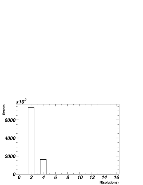
Figure 1: Number of solutions per event.

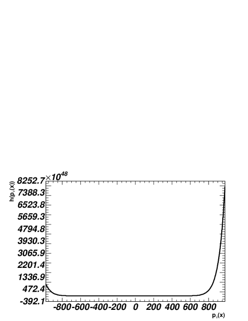
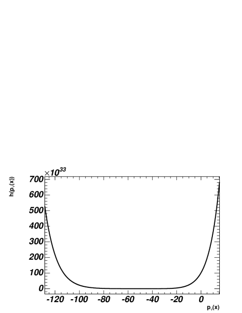
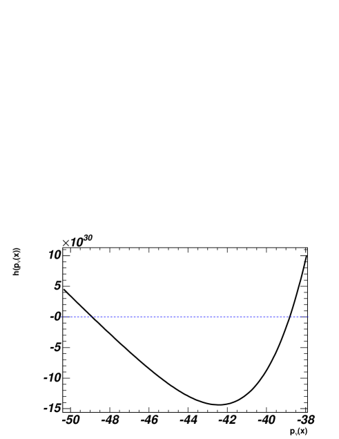
Figure 2: A typical univariate polynomial of degree 16 whose real roots in $p_{\nu_{x}}$ are solutions of the initial system of equations describing the $t\bar{t}$ dilepton kinematics. From top to bottom the plots are zoomed around the interesting $p_{\nu_{x}}$ range of the abscissa where two solutions are located.

(Now one could turn the way to solve a given Eigenvalue problem the other way around and use the Sturm sequence to solve the characteristic polynomial to obtain the Eigenvalues).

The neutrino and antineutrino masses are assumed to be zero in good approximation in the following. They have been kept in the equations for the sake of completeness since the same set of equations can be exploited in search for new physics with the same decay topology including invisible massive particles.

Once the solutions are found - most frequently there are two but never more than four (see fig. 1) - they can be inserted in equations (III). Such that these equations reduce to two univariate polynomials of degree four which in turn can be solved analytically to $p_{\nu_{y}}$ with a four fold ambiguity. The ambiguities can be eliminated in requiring the roots of these two polynomials to coincide since both equations have to be satisfied simultaneously. $p_{\bar{\nu}_{x}}$ and $p_{\bar{\nu}_{y}}$ can be simply determined with help of the first two equations in (II). To determine the longitudinal neutrino and antineutrino momenta $p_{\nu_{z}}$ and $p_{\bar{\nu}_{z}}$ the equations (III) and (III) can be evaluated respectively. Again the two-fold ambiguity, here due to the square root sign, can be resolved in requiring the solutions to coincide simultaneously for both equations of one parton branch.

IV Performance of the method

The univariate polynomial of $p_{\nu_{x}}$ is in general very shallow around zero over a broad range of neutrino momenta in comparison to its maximal values in the allowed kinematic range as can be concluded from the first two graphs in fig. 2. Here the kinematic range has been restricted to a centre of mass energy of 1.96 TeV, assuming the Tevatron proton anti-proton collider which has been set up in the Monte-Carlo event generator PYTHIA 6.220 PYTHIA used here. Cross checks at a centre of mass energy of 14 TeV assuming the LHC proton proton collider environment confirm that the performance is independent of particular collider settings. Only when in the graphs the area of the abscissa is zoomed very close to the solutions they can be recognised by eye. At this level the ordinate has already been magnified by 20 orders of magnitude. This explains why it is in general so difficult to find any solutions with numerical methods.

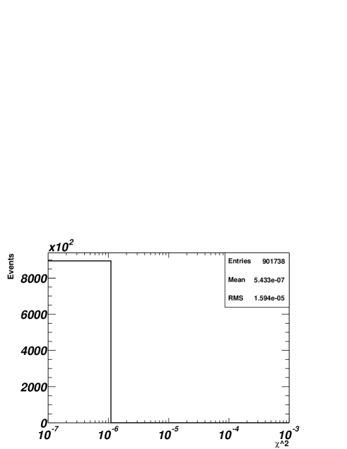
Figure 3: Solution $\chi^{2}$ defined as the difference between solved and generated neutrino momenta, added in quadrature, for the closest solution of each event.

In 99.9% of the events a solution can be found which is shown in the number of solutions per event distribution of fig. 1. The neutrino momenta $p_{\nu}^{sol}$ of the solutions are compared to the generated ones $p_{\nu}^{gen}$ by defining a metric $\chi$ through

$$\chi^{2} = (p_{\nu_{x}}^{gen}\!-p_{\nu_{x}}^{sol})^{2}+(p_{\nu_{y}}^{gen}\!-p_{\nu_{y}}^{sol})^{2}+(p_{\nu_{z}}^{gen}\!-p_{\nu_{z}}^{sol})^{2}$$

$$+ (p_{\bar{\nu}_{x}}^{gen}\!-p_{\bar{\nu}_{x}}^{sol})^{2}+(p_{\bar{\nu}_{y}}^{gen}\!-p_{\bar{\nu}_{y}}^{sol})^{2}+(p_{\bar{\nu}_{z}}^{gen}\!-p_{\bar{\nu}_{z}}^{sol})^{2}\;.$$

Figure 4: Minimal solution $\chi^{2}$ per event. The first two plots differ in parton information entered into the solving procedure: a) top quark pole and $W$ boson off-shell masses, b) top quark and $W$ boson pole masses. The two lower plots show $\chi^{2}$ distributions of reconstructed events, considering both $b$ jet permutations with reconstructed jets in c) and additionally smearing applied to jets and leptons in d).

	Solution
Condition	Efficiency	Purity	Mean $\chi^{2}$
$W$ mass known exactly
$t$ pole mass assumed	0.893	$5.21\cdot 10^{-5}$	417.3
$t,W$ pole mass assumed	0.839	0	911.0
$t,W$ pole mass assumed
both $b\bar{b}$ permutations	0.890	0	1166
reconstructed $b$-jets
(parton matched)	0.711	0	3916
wrong $b$-jet permutation
(parton matched)	0.426	0	5366
both $b$-jet permutations
(parton matched)	0.822	0	4049
both $b$-jet permutations
(parton matched,	0.761	0	4491
jets + leptons smeared)
both $b$-jet permutations
(parton matched,
jets + leptons smeared),	0.994	0	2556
reconstructed objects
100 times resolution smeared

Table 1: Solutions fulfilling $\chi^{2}<10^{-3}$ are defined as matched and else unmatched. The purity is determined according to this definition. The Mean $\chi^{2}$ is obtained taking into account matched and unmatched events.

The solutions coincide in 99.7% of cases within real precision to the generated neutrino momenta. Fig. 3 shows impressively how accurate and reliably the method is working. The plots in fig. 4 show the $\chi^{2}$ distribution on a linear scale. Since in practice the off-shell masses of the top quark and $W$ boson resonances are not known the method has been applied in the following ways: The distribution in the first plot assumes $W$ boson off-shell but top quark pole masses. It peaks at zero and its tail vanishes rapidly. The solution efficiency for this scenario amounts to 89%. The second plot assumes the pole mass for the top quarks and the $W$ bosons. The number and mean of unmatched solutions increases dramatically and the efficiency drops to 84%. Further an infrared-safe cone algorithm H (1) with cone size $R=0.5$ in the space spanned by pseudorapidity and azimuthal angle has been applied to the hadronic final state particles to investigate the effect of reconstructed objects on the solutions. Requiring exactly two jets and two leptons and accepting the jets as $b$-tagged if they coincide within $\Delta R<0.5$ with the $b$ quarks and antiquarks yields an significant degradation of the $\chi^{2}$ distribution (fig. 4 c)). The efficiency drops to 43% assuming the right jet quark combination. Admitting both permutations yields an efficiency of 82%. The last plot has been obtained from the previous one in additionally smearing the leptons and jets with the energy resolution of the D$\emptyset$ detector D . The $\chi^{2}$ of the minimal solution suffers in average another ten percent degradation and the solution efficiency drops by the same amount. In practice a given event passes the solving procedure repeatedly to improve the solution efficiency. Each iteration the energy of the reconstructed objects is randomly drawn from a probability distribution describing the detector resolution and centred around the measured values. In the case of hundred such iterations the efficiency can be kept above 99.4% while in average the $\chi^{2}$ of the best solution decreases considerably as expected in comparison to solving the momenta of the reconstructed objects just once.

In table 1 the efficiencies and minimal solution $\chi^{2}$’s are summarised. In addition the purity is given. It is practically zero, which means that no solutions do match with real precision or even merely with a $\chi^{2}$ better than $10^{-3}$ once the off-shell masses of the top quarks and $W$ bosons are not assumed to be known exactly.

General numerical methods can compare and gauge their performance in terms of solution efficiency and purity with the algebraic approach described here.

The time consumption of the method amounts to about 20% of the time needed for the generation of the events which means if $5\cdot 10^{6}$ events can be generated in five hours an additional hour is needed to solve them. The strength of the method is the application of Sturm’s theorem, such that in the case of no solutions the time consuming seeking and polishing of solutions can be saved. The bottleneck of the method is the time consuming evaluation of the resultant.

V Conclusions

An algebraic approach to solve the $t\bar{t}$ dilepton kinematics has been presented. The system of equations can be reduced to a univariate polynomial by means of resultants. The number of real roots can be determined by means of Sturm’s theorem. Once the single roots have been isolated they can be polished by binary bracketing while seeking for the sign change. In this way a solution is found in 99.9% of cases. The solutions coincide with real precision to the generated neutrino energies and momenta in 99.7% of cases assuming that the reconstructible parton momenta inserted in the solving procedure are known exactly. Little deviations drop the solution efficiency considerably, at the order of tens of percent. In this case the solved neutrino momenta differ already in average by the order of tens of GeV from the generated parton momenta. The solution efficiency can be re-established above the 99% level in solving a given event several times, varying the energy of the reconstructed objects each iteration randomly according to the energy resolution of a detector. General numerical methods can compare their performance in terms of efficiency and purity to the algebraic approach whose implementation has been described here.

Coefficients

Before defining the coefficients of equations (III) and (III) it is useful to introduce the following invariant masses

$$m_{\ell^{+}} = \sqrt{E_{\ell^{+}}^{2}-p_{\ell^{+}_{x}}^{2}-p_{\ell^{+}_{y}}^{2}-p_{\ell^{+}_{z}}^{2}}$$

$$m_{\ell^{-}} = \sqrt{E_{\ell^{-}}^{2}-p_{\ell^{-}_{x}}^{2}-p_{\ell^{-}_{y}}^{2}-p_{\ell^{-}_{z}}^{2}}$$

$$m_{b} = \sqrt{E_{b}^{2}-p_{b_{x}}^{2}-p_{b_{y}}^{2}-p_{b_{z}}^{2}}$$

$$m_{\bar{b}} = \sqrt{E_{\bar{b}}^{2}-p_{\bar{b}_{x}}^{2}-p_{\bar{b}_{y}}^{2}-p_{\bar{b}_{z}}^{2}}$$

$$m_{b\ell^{+}} = \left\{(E_{b}+E_{\ell^{+}})^{2}-(p_{b_{x}}+p_{\ell^{+}_{x}})^{2}\right.$$

$$\left.-(p_{b_{y}}+p_{\ell^{+}_{y}})^{2}-(p_{b_{z}}+p_{\ell^{+}_{z}})^{2}\right\}^{\frac{1}{2}}$$

$$m_{\bar{b}\ell^{-}} = \left\{(E_{\bar{b}}+E_{\ell^{-}})^{2}-(p_{\bar{b}_{x}}+p_{\ell^{-}_{x}})^{2}\right.$$

$$\left.-(p_{\bar{b}_{y}}+p_{\ell^{-}_{y}})^{2}-(p_{\bar{b}_{z}}+p_{\ell^{-}_{z}})^{2}\right\}^{\frac{1}{2}}$$

The coefficients are then given by

$$a_{11} = \frac{1}{2}\frac{(m_{W^{+}}^{2}-m_{\ell^{+}}^{2}-m_{\nu}^{2})p_{\ell^{+}_{z}}}{E_{\ell^{+}}^{2}-p_{\ell^{+}_{z}}^{2}}$$

$$a_{12} = \frac{p_{\ell^{+}_{x}}p_{\ell^{+}_{z}}}{E_{\ell^{+}}^{2}-p_{\ell^{+}_{z}}^{2}}$$

$$a_{13} = \frac{p_{\ell^{+}_{y}}p_{\ell^{+}_{z}}}{E_{\ell^{+}}^{2}-p_{\ell^{+}_{z}}^{2}}$$

$$a_{21} = \frac{1}{4(E_{\ell^{+}}^{2}-p_{\ell^{+}_{z}}^{2})}\cdot\left(m_{W^{+}}^{4}+m_{\ell^{+}}^{4}+m_{\nu}^{4}\right.$$

$$\left.-2m_{W^{+}}^{2}m_{\ell^{+}}^{2}-2m_{W^{+}}^{2}m_{\nu}^{2}+2m_{\ell^{+}}^{2}m_{\nu}^{2}\right)$$

$$a_{22} = \frac{(m_{W^{+}}^{2}-m_{\ell^{+}}^{2}-m_{\nu}^{2})p_{\ell^{+}_{x}}}{E_{\ell^{+}}^{2}-p_{\ell^{+}_{z}}^{2}}$$

$$a_{23} = \frac{(m_{W^{+}}^{2}-m_{\ell^{+}}^{2}-m_{\nu}^{2})p_{\ell^{+}_{y}}}{E_{\ell^{+}}^{2}-p_{\ell^{+}_{z}}^{2}}$$

$$a_{24} = -\frac{E_{\ell^{+}}^{2}-p_{\ell^{+}_{x}}^{2}}{E_{\ell^{+}}^{2}-p_{\ell^{+}_{z}}^{2}}$$

$$a_{25} = \frac{2p_{\ell^{+}_{x}}p_{\ell^{+}_{y}}}{E_{\ell^{+}}^{2}-p_{\ell^{+}_{z}}^{2}}$$

$$a_{26} = -\frac{E_{\ell^{+}}^{2}-p_{\ell^{+}_{y}}^{2}}{E_{\ell^{+}}^{2}-p_{\ell^{+}_{z}}^{2}}\;.$$

To obtain the coefficients $c_{mn}$ for the other parton branch one has to substitute $W^{+}$, $\ell^{+}$ and $\nu$ by $W^{-}$, $\ell^{-}$ and $\bar{\nu}$ respectively. Similar holds

$$b_{11} = \frac{1}{2}\frac{(m_{t}^{2}-m_{b\ell^{+}}^{2}-m_{\nu}^{2})(p_{b_{z}}+p_{\ell^{+}_{z}})}{(E_{b}+E_{\ell^{+}})^{2}-(p_{b_{z}}+p_{\ell^{+}_{z}})^{2}}$$

$$b_{12} = \frac{(p_{b_{x}}+p_{\ell^{+}_{x}})(p_{b_{z}}+p_{\ell^{+}_{z}})}{(E_{b}+E_{\ell^{+}})^{2}-(p_{b_{z}}+p_{\ell^{+}_{z}})^{2}}$$

$$b_{13} = \frac{(p_{b_{y}}+p_{\ell^{+}_{y}})(p_{b_{z}}+p_{\ell^{+}_{z}})}{(E_{b}+E_{\ell^{+}})^{2}-(p_{b_{z}}+p_{\ell^{+}_{z}})^{2}}$$

$$b_{21} = \frac{1}{4((E_{b}+E_{\ell^{+}})^{2}-(p_{b_{z}}\!\!+p_{\ell^{+}_{z}})^{2})}\cdot\left(m_{t}^{4}+m_{b\ell^{+}}^{4}\!+m_{\nu}^{4}\right.$$

$$\left.-2m_{t}^{2}m_{b\ell^{+}}^{2}-2m_{t}^{2}m_{\nu}^{2}+2m_{b\ell^{+}}^{2}m_{\nu}^{2}\right)$$

$$b_{22} = \frac{(m_{t}^{2}-m_{b\ell^{+}}^{2}-m_{\nu}^{2})(p_{b_{x}}+p_{\ell^{+}_{x}})}{(E_{b}+E_{\ell^{+}})^{2}-(p_{b_{z}}+p_{\ell^{+}_{z}})^{2}}$$

$$b_{23} = \frac{(m_{t}^{2}-m_{b\ell^{+}}^{2}-m_{\nu}^{2})(p_{b_{y}}+p_{\ell^{+}_{y}})}{(E_{b}+E_{\ell^{+}})^{2}-(p_{b_{z}}+p_{\ell^{+}_{z}})^{2}}$$

$$b_{24} = -\frac{(E_{b}+E_{\ell^{+}})^{2}-(p_{b_{x}}+p_{\ell^{+}_{x}})^{2}}{(E_{b}+E_{\ell^{+}})^{2}-(p_{b_{z}}+p_{\ell^{+}_{z}})^{2}}$$

$$b_{25} = \frac{2(p_{b_{x}}+p_{\ell^{+}_{x}})(p_{b_{y}}+p_{\ell^{+}_{y}})}{(E_{b}+E_{\ell^{+}})^{2}-(p_{b_{z}}+p_{\ell^{+}_{z}})^{2}}$$

$$b_{26} = -\frac{(E_{b}+E_{\ell^{+}})^{2}-(p_{b_{y}}+p_{\ell^{+}_{y}})^{2}}{(E_{b}+E_{\ell^{+}})^{2}-(p_{b_{z}}+p_{\ell^{+}_{z}})^{2}}\;.$$

Again the coefficients $d_{mn}$ of the other parton branch can be obtained in substituting $t$, $b$, $\ell^{+}$ and $\nu$ by $\bar{t}$, $\bar{b}$, $\ell^{-}$ and $\bar{\nu}$ respectively. The denominators are always of the type

$$E^{2}-p_{z}^{2}=m^{2}+p_{\perp}^{2}\geq m^{2}\;.$$

Thus it is ensured that they never vanish. Running over 1 million Monte-Carlo events does not lead to a division by zero. In addition, detected objects in collider experiments have always a considerable amount of transverse momentum which pushes the kinematics of the equations further away from such singularities. Therefore the theoretically possible multiplication of all equations with the least common multiple of all denominators does not need to be applied.

References

• (1) R. H. Dalitz, G. R. Goldstein, β€œDecay and polarization properties of the top quark”, Nuclear Physics D 45 (1992) 5-1531.
• (2) Waterloo Maple Inc., Maple 9.5, 2004.
• (3) Eric W. Weisstein., β€œQuintic Equation”, From MathWorld–A Wolfram Web Resource, http://mathworld.wolfram.com/QuinticEquation.html, 1995
• (4) Rene Brun, Fons Rademakers, β€œRoot 4”, http://root.cern.ch, 2004
• (5) Thomas Becker, Volker Weispfenning, β€œGrΓΆbner Bases”, Springer Verlag, 1993
• (6) D. E. Knuth, β€œThe Art of Computer Programming, Vol. 2”, 3rd ed., Addison-Wesley, 1998 Β
• (7) http://fr.wikipedia.org/wiki/Charles_Sturm, 2005
• (8) T. SjΓΆstrand, P. Eden, C. Friberg, L. LΓΆnnblad, G. Miu, S. Mrenna and E. Norrbin, Computer Physics Commun. 135 (2001) 238.
• H (1) H1 Collab., C. Adloff et al, β€œMeasurement of internal jet structure in dijet production in deep-inelastic scattering at HERA”, Nuclear Physics B 545 (1999) 3-20.
• D (0) S. N. Fatakia, U. Heintz, L. Sonnenschein, β€œTop Mass Measurement in the Dilepton Channel”, D$\emptyset$ note 4677