Bound State versus Collective Coordinate Approaches in Chiral Soliton Models and the Width of the $\Theta^{+}$ Pentaquark

Abstract

We thoroughly compare the bound state and rigid rotator approaches to three–flavored chiral solitons. We establish that these two approaches yield identical results for the baryon spectrum and kaon–nucleon $S$–matrix in the limit that the number of colors ($N_{C}$) tends to infinity. After proper subtraction of the background phase shift the bound state approach indeed exhibits a clear resonance behavior in the strangeness $S=+1$ channel. We present a first dynamical calculation of the widths of the $\Theta^{+}$ and $\Theta^{*}$ pentaquarks for finite $N_{C}$ in a chiral soliton model.

I Introduction

Chiral soliton model predictions for the mass of the lightest exotic pentaquark, the $\Theta^{+}$ with zero isospin and unit strangeness, have been around for about two decades Ma84 ; Bi84 ; Ch85 ; Pr87 ; Wa92 ; Wa92a . Nevertheless, the study of such pentaquarks as potential baryon resonances became popular only a short while ago when experiments Na03 indicated their existence. These experiments were stimulated by a chiral soliton model estimate that claimed that the width of the pentaquark decaying into a kaon and a nucleon would be much smaller than those typical for hadronic decays of baryon resonances Di97 ; Pr03 ; Pr04 , however, see also Ja04 . Such narrow resonances could have escaped detection in earlier analyses.

I.1 Hadronic Decays in Soliton Models

Estimates for the $\Theta^{+}$ width are based on identifying the interpolating kaon field with the (divergence) of the axial current, which in turn is computed solely from the classical soliton. This is essentially a generalization to flavor $SU(3)$ of the early calculation of the $\Delta\to\pi N$ decay width in the pioneering paper of ref. Ad83 in the two flavor Skyrme model. Since then there have been quite some efforts to understand that process in chiral soliton models by going beyond the simple identification of the pseudoscalar meson fields with the axial current Ue85 ; Sa87 ; Ho87 ; Ve88 ; Di88 ; Ho90 ; Ho90a ; Ha90 ; Do94 ; see also chapter IV in ref. Ho93 . It must be stressed that the description of hadronic decays in soliton models is a severe problem and has become known as the Yukawa problem in soliton models. The reason is that the interaction Hamiltonian that mediates such hadronic transitions must be linear in the field operator that corresponds to the pseudoscalar meson in the final state. On the other hand the naïve definition of the soliton as a stationary point of the action prohibits such a linear term. Hence in these models resonance widths must be extracted from appropriate $S$–matrix elements of meson baryon scattering. Most of the studies on meson baryon scattering are restricted to the adiabatic approximation Wa84 ; Ha84 ; Kr86 ; Schw89 which represents the next–to–leading order in the $1/N_{C}$ expansion where $N_{C}$ is the number of colors. Unfortunately in the large–$N_{C}$ limit the $\Delta$ is degenerate with the nucleon and its width is of even lower order in that expansion. Therefore its width cannot be computed in adiabatic approximation and the above cited studies mainly motivate Born contributions to the $S$–matrix element of pion nucleon scattering in the $P_{33}$ channel at ${\cal O}(1/N_{C})$. For the pentaquarks the situation is very different. As we will see, the $\Theta^{+}$–nucleon mass difference is non–zero even as $N_{C}\to\infty$ and hence its hadronic decay width should be at the same order as the adiabatic approximation for kaon–nucleon scattering. In that respect the hadronic decays of pentaquarks are a perfect playground as any treatment that induces Born contributions can be tested against the adiabatic approximation.

I.2 Quantizing the Soliton in Flavor $\mathbf{SU(3)}$

When treating chiral solitons in flavor $SU(3)$ we face the problem how to properly generate baryon states from the classical soliton. Essentially there are two methods at our disposal, the bound state approach (BSA) Ca85 and the rigid rotator approach (RRA) Gu84 ; see e.g. ref. We96 for a review and further references. The latter is essentially the generalization of the collective coordinate quantization adopted earlier for the two flavor model Ad83 . In this approach collective coordinates that describe the spin flavor orientation of the soliton are introduced and quantized canonically. As this corresponds to quantizing a rigid top in $SU(3)$ it is natural that the corresponding eigenstates are characterized according to $SU(3)$ multiplets, most prominently the octet ($\mathbf{8}$) and decuplet ($\mathbf{10}$) for baryons with spin $J=\frac{1}{2}$ and $J=\frac{3}{2}$, respectively. However, also more exotic $SU(3)$ representations like the anti–decuplet ($\overline{\mathbf{10}}$) emerge. In addition to states with quantum numbers of octet baryons this representation also contains states with quantum numbers that cannot be built as three–quark composites. These states contain (at least) one additional quark–antiquark pair which lead to the notion of exotic pentaquarks. Most prominently there have been experimental claims Na03 ; Hi04 ; Ka05 for a $\Theta^{+}$ pentaquark, the strangeness $S=+1$ isosinglet that sits at the top of the anti–decuplet.

In the BSA kaon fluctuations $\eta_{\alpha}(\vec{x\,},t)$, with $\alpha=4,\ldots,7$, are introduced and quantized as harmonic oscillations. It corresponds to the adiabatic approximation and should be exact as $N_{C}\to\infty$. Common to all soliton models is the appearance of a bound state with strangeness $S=-1$ which serves to construct states that correspond to the ordinary hyperons, $\Lambda$, $\Sigma$ and $\Sigma^{*}$. On the other hand neither a bound state nor a clear resonance has been observed in the $S=+1$ channel. This non–observation has often been used to argue that the pentaquark prediction would be a mere artifact of the RRA It03 ; Co03 ; Ch05 . Here we will show that this statement is completely based on a misinterpretation of the RRA. For a sensible and ultimate comparison of the BSA and the RRA it is necessary to also include small amplitude fluctuations in the RRA. We call that approach the rotation–vibration approach (RVA). However, the fluctuations in the RVA must be constrained to the subspace that is orthogonal to the rigid rotation. We therefore label these fluctuation by $\overline{\eta}_{\alpha}(\vec{x\,},t)$. Then the test mentioned at the end of subsection A is to first compute the $S$–matrix from the constrained fluctuations, $\overline{\eta}_{\alpha}(\vec{x\,},t)$ and supplement that result with the contributions from the (iterated) $\Theta^{+}$ exchange. That yields the wave–functions $\widetilde{\eta}_{\alpha}(\vec{x\,},t)$ that are constrained to the same subspace as $\overline{\eta}_{\alpha}(\vec{x\,},t)$. The $\widetilde{\eta}_{\alpha}(\vec{x\,},t)$ are the full solution to the RVA. In the limit $N_{C}\to\infty$  $\widetilde{\eta}_{\alpha}(\vec{x\,},t)$ must yield the same $S$–matrix as in the BSA, i.e. when extracted from ${\eta}_{\alpha}(\vec{x\,},t)$. In performing this test, our studies serve three major purposes: First, we will establish the equivalence of BSA and RVA in the large–$N_{C}$ limit. Second, we will compare $\widetilde{\eta}_{\alpha}$ and $\overline{\eta}_{\alpha}$ to extract a distinct $S=1$ resonance in kaon nucleon scattering that survives as $N_{C}\to\infty$. Third, we will provide the first dynamical calculation of the $\Theta^{+}$ width in a chiral soliton model for finite $N_{C}$.

I.3 General Remarks

Let us round off this introduction section with a few general remarks on the comparison between the BSA, the RRA and the RVA. Generally we may always introduce collective coordinates to investigate specific excitations. This is irrespective of whether the corresponding excitation energies are suppressed in the large–$N_{C}$ limit or not. That is, in contrast to the claims of refs. Co03 no separation of scales is required to validate the collective coordinate quantization. Eventually the coupling terms and constraints ensure correct results. Even more, we will observe in section V that collective coordinates may also be introduced for $m_{K}\neq m_{\pi}$. This result generalizes to the statement that collective coordinates are not necessarily linked to the zero–modes of a system and any distinction between dynamical and static zero–modes Ch05 is obsolete. Already some time ago the concept of describing baryon resonances as collective excitations has been successfully applied to quadrupole Ha84a and monopole excitations, both in two Ha84b and three Sch91a flavor models. In particular collective monopole excitations have been studied in the context of the pentaquark excitation We98 ; We04 .

Sometimes the correct description of the $\Lambda(1405)$ as an $S$–wave bound state is considered as an argument in favor of the BSA vs. the RRA. Again it must be stressed that the full RVA also contains kaon fluctuations and thus also describes the formation of an $S$–wave bound state. As shown in ref. Schw91 this properly accounts for the $\Lambda(1405)$ in the RVA.

I.4 Outline

This paper is organized as follows. In section II we will define the model and describe the field parameterization in the bound state and rigid rotator approaches in more detail. In sections III and IV we extensively compare these approaches and show how they yield identical spectra in the limit $N_{C}\to\infty$, even for non–zero symmetry breaking, when the fluctuating modes are limited to the same subspace. In section III we also show that the constraints for $\overline{\eta}_{\alpha}$ serve to separate resonance and background pieces of the phase shift. Section V represents a main piece of our paper as we combine rotational and fluctuation degrees of freedom to construct the solution for the RVA up to quadratic order in the fluctuations. We employ this solution to compute the width of the $\Theta^{+}$ pentaquark for $m_{K}=m_{\pi}$ in section VI. Another major result is that in the flavor symmetric case only a single collective coordinate operator mediates the transition $\Theta^{+}\to KN$ at the leading order of the large–$N_{C}$ expansion. This is in direct contradiction to approaches that construct transition interactions with (at least) two $SU(3)$ operators and adjust the coefficients to yield a narrow $\Theta^{+}$ Di97 ; Pr03 ; El04 ; Pr05 . In section VII we extend our treatment to the physical case $m_{K}\neq m_{\pi}$. This brings a second $SU(3)$ operator into the game. In section VIII we collect our numerical results and summarize in section IX. We relegate technical details on the derivation of the equation of motion for the constrained fluctuations to an appendix.

II The Model

For simplicity we consider the Skyrme model Sk61 as a particular example for chiral soliton models. However, we stress that our qualitative results do indeed generalize to all chiral soliton models because these results solely originate from the treatment of the model degrees of freedom.

A preliminary remark on notation: In what follows we adopt the convention that repeated indices are summed over in the range

$$\begin{array}[b]{lcll}a,b,c,\ldots&=&1,\ldots,8&\cr\alpha,\beta,\gamma,\ldots&=&4,\ldots,7&{\rm(kaonic)}\cr i,j,k,\ldots&=&1,2,3&{\rm(pionic)}\,.\end{array}$$ (1)

Chiral soliton models are functionals of the chiral field, $U$, the non–linear realization of the pseudoscalar mesons, $\phi_{a}$

$$U(\vec{x\,},t)={\rm exp}\left[\frac{i}{f_{\pi}}\phi_{a}(\vec{x\,},t)\lambda_{a}\right]\,,$$ (2)

with $\lambda_{a}$ being the Gell–Mann matrices of $SU(3)$. For a convenient presentation of the model we split the action into three pieces

$$\Gamma=\Gamma_{SK}+\Gamma_{WZ}+\Gamma_{SB}\,.$$ (3)

The first term represents the Skyrme model action

$$\Gamma_{SK}=\int d^{4}x\,{\rm tr}\,\left\{\frac{f^{2}_{\pi}}{4}\left[\partial_{\mu}U\partial^{\mu}U^{\dagger}\right]+\frac{1}{32\epsilon^{2}}\left[[U^{\dagger}\partial_{\mu}U,U^{\dagger}\partial_{\nu}U]^{2}\right]\right\}\,.$$ (4)

Here $f_{\pi}=93{\rm MeV}$ is the pion decay constant and $\epsilon$ is the dimensionless Skyrme parameter. In principle this is a free model parameter. The two–flavor version of the Skyrme model suggests to put $\epsilon=4.25$ from reproducing the $\Delta$–nucleon mass difference. The anomaly structure of QCD is incorporated via the Wess–Zumino action Wi83

$$\Gamma_{WZ}=-\frac{iN_{C}}{240\pi^{2}}\int d^{5}x\ \epsilon^{\mu\nu\rho\sigma\tau}{\rm tr}\,\left[L_{\mu}L_{\nu}L_{\rho}L_{\sigma}L_{\tau}\right]\,,$$ (5)

with $L_{\mu}=U^{\dagger}\partial_{\mu}U$. Note that $\Gamma_{WZ}$ vanishes in the two–flavor version of the model. Furthermore $N_{C}$ is the number of colors, the hidden expansion parameter of QCD tH74 ; Wi79 .

The flavor symmetry breaking terms are contained in $\Gamma_{\rm SB}$

$$\Gamma_{SB}=\frac{f_{\pi}^{2}}{4}\,\int d^{4}x\,{\rm tr}\,\left[{\cal M}\left(U+U^{\dagger}-2\right)\right]\qquad{\rm with}\qquad{\cal M}=\begin{pmatrix}m_{\pi}^{2}&0&0\cr 0&m_{\pi}^{2}&0\cr 0&0&2m_{K}^{2}-m_{\pi}^{2}\end{pmatrix}\,.$$ (6)

Unless otherwise stated we will adopt the empirical data for the masses of the pseudoscalar mesons: $m_{\pi}=138{\rm MeV}$ and $m_{K}=495{\rm MeV}$. We do not include terms that distinguish between pion and kaon decay constants even though they differ by about 20% empirically. This is a mere matter of convenience rather than negligence. This omission leads to a considerable underestimation of symmetry breaking effects We90 which approximately can be accounted for by rescaling the kaon mass $m_{K}\to m_{K}f_{K}/f_{\pi}$.

Although physically sensible results are obtained by setting $N_{C}=3$, it is very illuminating to organize the calculation in powers of $1/N_{C}$ and consider $N_{C}$ undetermined. In the context of this $N_{C}$ counting the mass parameters are ${\cal O}(N_{C}^{0})$ while $f_{\pi}={\cal O}(\sqrt{N_{C}})$ and $\epsilon={\cal O}(1/\sqrt{N_{C}})$ to ensure that the (perturbative) $n$–point functions scale as $N_{C}^{1-n/2}$ Wi79 . In order to study the $N_{C}$ dependence in the three flavor version of the soliton model we include the $N_{C}$ dependence in the choice of the model parameters via

$$f_{\pi}=93{\rm MeV}\sqrt{\frac{N_{C}}{3}}\quad{\rm and}\quad\epsilon=4.25\sqrt{\frac{3}{N_{C}}}\,.$$ (7)

The action, eq. (3) allows for a topologically non–trivial classical solution, the famous hedgehog soliton

$$U_{0}(\vec{x\,})={\rm exp}\left[i\vec{\lambda\,}\cdot\hat{x}F(r)\right]\,,\quad r=|\vec{x\,}|$$ (8)

which is embedded in the isospin subspace of flavor $SU(3)$ parameterized by the Gell–Mann matrices $\lambda_{i}$, $i=1,2,3$. Other embeddings are possible but energetically disfavored due to flavor symmetry breaking. The chiral angle, $F(r)$ is obtained from integrating the classical equation of motion extracted from eqs. (4) and (6) subject to the boundary condition $F(0)-F(\infty)=\pi$ ensuring unit winding (baryon) number. The soliton can be constructed as a function of the dimensionless variable $\epsilon f_{\pi}r$ and is thus not subject to $N_{C}$ scaling.

The excitations of this soliton configuration are quantized to generate physical baryon states. The central task in extending this picture to three flavors is the incorporation of strange degrees of freedom, that is kaons. In a first step we introduce fluctuations $\eta_{a}(\vec{x\,},t)$ with $a=1,\ldots,8$, for the pseudoscalar fields Ca85 ; Ca88 ; Kl89 ,

$$U(\vec{x\,},t)=\sqrt{U_{0}(\vec{x\,})}\,{\rm exp}\left[\frac{i}{f_{\pi}}\lambda_{a}\eta_{a}(\vec{x\,},t)\right]\sqrt{U_{0}(\vec{x\,})}\,.$$ (9)

Expanding the action in powers of these fluctuations actually is an expansion in $\eta_{a}/f_{\pi}$ and thus a systematic series in $1/\sqrt{N_{C}}$. The term quadratic in $\eta_{a}$ is of special interest. It describes scattering of mesons off a potential that is generated by the classical soliton, eq. (8). In particular an anti–kaon is bound in the $P$–wave channel. Combined with the soliton it may be interpreted as the $\Lambda$ hyperon. However, the system consisting of the soliton and this bound anti–kaon has still to be projected onto states with good spin and isospin. This is accomplished by introducing collective coordinates for the spin–isospin orientation, $A_{2}(t)\in SU(2)$

$$U(\vec{x\,},t)=A_{2}(t)\sqrt{U_{0}(\vec{x\,})}\,{\rm exp}\left[\frac{i}{f_{\pi}}\lambda_{a}\eta_{a}(\vec{x\,},t)\right]\sqrt{U_{0}(\vec{x\,})}\,A_{2}^{\dagger}(t)\,$$ (10)

and quantizing them canonically Ca85 ; Kl89 . In this treatment the kaon fluctuations $a=\alpha=4,\ldots,7$ decouple in the adiabatic equations of motion. This leads to the so–called bound state approach (BSA) that we will review in section III.

The seemingly alternative approach is to allow the collective coordinates to span the full flavor space, $A_{3}(t)\in SU(3)$ and quantize $A_{3}$ canonically to generate baryon states with non–zero strangeness while omitting the fluctuations. Baryon states are then classified according to $SU(3)$ representations. This is the so–called rigid rotator approach (RRA) Gu84 . However, for a sensible investigation of the rotation–vibration coupling the collective coordinate approach must be completed to also contain meson fluctuations. Hence the ansatz that defines the RVA reads

$$U(\vec{x\,},t)=A_{3}(t)\sqrt{U_{0}(\vec{x\,})}\,{\rm exp}\left[\frac{i}{f_{\pi}}\lambda_{a}\widetilde{\eta}_{a}(\vec{x\,},t)\right]\sqrt{U_{0}(\vec{x\,})}\,A_{3}(t)^{\dagger}\,.$$ (11)

Obviously eq. (11) comprises the ansatz, eq. (10). In contrast to eq. (10) the ansatz (11) has additional collective rotations into strange directions. But these field components are also contained in the fluctuations, $\widetilde{\eta}_{\alpha}$. It is therefore necessary to constrain these fluctuations to the subspace that is orthogonal to the rigidly rotating hedgehog. These constraints modify the equations of motion for the fluctuations, such that $\widetilde{\eta}_{\alpha}\neq\eta_{\alpha}$. This is not new: In principle we encounter the same problem already in $SU(2)$ where the ansätze eqs. (10) and  (11) are identical. The difference to the $SU(3)$ case is that the redundant modes are automatically orthogonal to the rigid rotations when treating the $SU(2)$ model in adiabatic approximation. This changes, however, as soon as non–adiabatic contributions or external fields e.g. photons Me97 , are considered. We will discuss and derive the modifications that occur in the $SU(3)$ case in section III and a separate appendix, respectively.

It is obvious that the ansätze (10) and (11) span the same Fock space in the baryon number one sector. An essential difference, however, is that an expansion to a given order in $\eta_{a}$ using eq. (10) contains the kaon fields only up to a fixed power in the $1/N_{C}$ expansion while the ansatz (11) treats the collective rotations to all orders. Obviously the two treatments must yield identical results in the limit $N_{C}\to\infty$. This provides a thorough check on our calculations. We also stress that the RVA formulation induces terms in the action that are linear in $\widetilde{\eta}_{\alpha}$ (in contrast the BSA does not give terms linear in $\eta_{\alpha}$). This gives rise to Yukawa couplings from which we will evaluate widths of rotational excitations.

There have been earlier studies of the non–adiabatic rotation–vibration coupling in the Skyrme model. In the $SU(2)$ version the contribution linear in the time derivative of $A_{2}$ has been shown to properly describe the Tomozawa–Weinberg relations for $S$–wave pion nucleon scattering Wa91 . Also in the two flavor model, the terms quadratic in the time derivative of the collective coordinates have been employed to incorporate thresholds and $\Delta$ resonance exchange effects in pion–nucleon scattering Ha90 ; Ho90 ; Ho90a ; Schw89 . In the three–flavor BSA the rotation–vibration coupling gives rise to the hyperfine mass splitting Kl89 that we will discuss in the following section. Also in $SU(3)$ meson baryon scattering has been investigated in the RVA Schw91 . Unfortunately, the strangeness, $S=+1$ channel, which contains the $\Theta^{+}$ pentaquark, was not considered in that outstanding paper.

III Bound state approach (BSA)

In this section we will discuss the construction of $P$–wave baryons with strangeness $S=\pm 1$ in the framework of the BSA starting from the parameterization, eq. (9). Baryons with zero strangeness are treated as in two–flavor chiral soliton models Ad83 .

III.1 Conventional BSA in the P–wave channel

As in refs. Ca85 ; Ca88 we expand the action to quadratic order in the kaonic fluctuations $\eta_{\alpha}$ in the background of the soliton, eq. (8). These wave–functions describe kaon–nucleon scattering in the intrinsic frame. In this frame the modes decouple with respect to grand spin ${\cal G}=\ell\pm\mbox{\small$\frac{1}{2}$}$, the eigenvalue of the sum of kaon orbital angular momentum ($\ell$) and isospin. This defines the intrinsic $T$–matrix, $T_{{\cal G},\ell}$. The $T$–matrix elements in the laboratory frame $T(\ell I2J)$ are linear combinations of the $T_{{\cal G},\ell}$ Ha84 ; Ma88 . For the $\Theta^{+}$ channel ($I=0$, $J=\frac{1}{2}$) this linear relation is very simple

$$T(P01)=T_{\frac{1}{2}1}$$ (12)

i.e. only the intrinsic $P$–wave kaon with grand spin ${\cal G}=\frac{1}{2}$ contributes. Its wave–function is characterized by a single radial function, that parametrically depends on the frequency in a Fourier analysis

$$\begin{pmatrix}\eta_{4}+i\eta_{5}\cr\eta_{6}+i\eta_{7}\end{pmatrix}_{P}(\vec{x\,},t)\,=\int_{-\infty}^{\infty}\,d\omega\,{\rm e}^{i\omega t}\,\eta_{\omega}(r)\,\hat{x}\cdot\vec{\tau}\,\chi(\omega)\,.$$ (13)

Here $\chi(\omega)$ is a two–component iso–spinor that contains the amplitudes of the kaon mode. Upon quantization its components will eventually be elevated to creation– and annihilation operators. Of course, an analogous decomposition exists for $\widetilde{\eta}_{\alpha}$ that defines the radial function $\widetilde{\eta}_{\omega}(r)$. In what follows we will omit the subscript $\omega$. The amplitude $\chi$ drops out from the equation of motion that can be formulated for the radial functions,

$$\Pi(r) = \left[\omega M_{K}(r)-\lambda(r)\right]\eta(r)\,,$$ (14)

$$h^{2}\eta(r)+\frac{\lambda^{2}(r)}{M_{K}(r)} = \left[\omega-\frac{\lambda(r)}{M_{K}(r)}\right]\Pi(r)\,.$$ (16)

Up to a factor $i$ the radial function $\Pi(r)$ parameterizes the momentum conjugate to the $P$–wave fluctuation Bl88 . The radial functions in eq. (16) can be taken from the literature Ca85 ; Ca88 ; Scha94 in terms of the chiral angle $F=F(r)$,

$$\lambda(r) = \frac{N_{C}}{4f_{\pi}^{2}}B_{0}(r)=-\frac{N_{C}}{8\pi^{2}f_{\pi}^{2}}F^{\prime}\,\frac{{\rm sin}^{2}F}{r^{2}}\,,\quad M_{K}(r)=1+\frac{1}{4f_{\pi}^{2}\epsilon^{2}}\left[F^{\prime 2}+2\frac{{\rm sin}^{2}F}{r^{2}}\right]\,$$ (17)

$$h^{2}\, = h^{2}_{0}\,+m_{K}^{2}-m_{\pi}^{2}\quad{\rm with}\quad h^{2}_{0}\,=-\frac{d^{2}}{dr^{2}}-\frac{2}{r}\frac{d}{dr}+V_{\rm eff}(r)\,,$$ (19)

where $F^{\prime}=\frac{dF(r)}{dr}$. The effective potential $V_{\rm eff}(r)$ is quite an involved function that also contains spatial derivative operators. Since it does not play any special role for our studies we do not repeat it here. The radial function $\lambda(r)$, proportional to the baryon density, $B_{0}(r)$, originates from the WZ–term, eq. (5) and thus contains the explicit factor $N_{C}$. The radial function $M_{K}(r)$ is the metric function for kaon fluctuations. This becomes obvious when eliminating the momentum $\Pi(r)$ in favor of a second order differential equation for $\eta(r)$,

$$h^{2}\,\eta(r)+\omega\left[2\lambda(r)-\omega M_{K}(r)\right]\eta(r)=0\,,$$ (20)

as $M_{K}(r)$ multiplies the term of highest power in the frequency, $\omega$. Eq. (20) could have been easily obtained without reference to the conjugate momentum. However, we have introduced it here because it becomes essential when implementing the constraints that characterize $\overline{\eta}$. The appearance of factors $N_{C}/f_{\pi}^{2}$ and $f_{\pi}^{2}\epsilon^{2}$ in the radial functions shows that $\eta(r)$ does not scale with $N_{C}$. Hence terms in the action that are of higher than quadratic order in $\eta_{\alpha}$ are suppressed due to the additional factor $1/f_{\pi}$. Thus solving eq. (20) provides the exact $T$–matrix in the limit $N_{C}\to\infty$.

The equation of motion (20) is not invariant under particle conjugation $\omega\leftrightarrow-\omega$, yielding different results for kaons ($\omega>0$) and anti–kaons ($\omega<0$). This difference obviously originates from the Wess–Zumino term. It is well known that equation (20) has a bound state solution at $\omega=-\omega_{\Lambda}$, that gives the mass difference between the $\Lambda$–hyperon and the nucleon in the large–$N_{C}$ limit. As this energy eigenvalue is negative it corresponds to a kaon, i.e. it carries strangeness $S=-1$. In the symmetric case ($m_{K}=m_{\pi}$) the bound state energy vanishes, i.e. the bound state is nothing but the zero mode of $SU(3)$ flavor symmetry. The radial function of the properly normalized zero mode reads

$$z(r)=\sqrt{4\pi}\frac{f_{\pi}}{\sqrt{\Theta_{K}}}\,{\rm sin}\frac{F(r)}{2}\quad{\rm with}\quad\Theta_{K}=f_{\pi}^{2}\int d^{3}r\,M_{K}(r)\,{\rm sin}^{2}\frac{F(r)}{2}=1.894{\rm GeV}^{-1}\left(\frac{N_{C}}{3}\right)\,.$$ (21)

It satisfies the important relation $h^{2}_{0}\,z(r)=0$. The normalization constant, $\Theta_{K}$ is the moment of inertia for flavor rotations into strangeness direction. In what follows we will employ the expressions ”zero–mode” and ”rotational mode” synonymously.

When symmetry breaking is switched on, the bound state evolves continuously from this zero mode. For $m_{K}=495{\rm MeV}$ we find $\omega_{\Lambda}=196{\rm MeV}$. This bound state energy can be reliably estimated by sandwiching the equation of motion (20) between zero mode wave–functions and solving for $\omega$. We first define

$$\omega_{0}=\int r^{2}drz^{2}(r)2\lambda(r)=\frac{N_{C}}{4\Theta_{K}}=0.396{\rm GeV}$$ (22)

and

$$\Gamma=\frac{8\Theta_{K}}{3}\left(m_{K}^{2}-m_{\pi}^{2}\right)\int r^{2}dr\,z^{2}(r)=2.969{\rm GeV}^{-1}\,\left(m_{K}^{2}-m_{\pi}^{2}\right)\,\frac{N_{C}}{3}\,,$$ (23)

which are ${\cal O}(N_{C}^{0})$ and ${\cal O}(N_{C})$, respectively. Then the equation for $\omega$ reads

$$\omega^{2}=\frac{3\Gamma}{8\Theta_{K}}+\omega_{0}\,\omega\,.$$ (24)

This quadratic equation for $\omega$ has the negative valued solution $-\omega_{\Lambda}$ with

$$\omega_{\Lambda}=\frac{1}{2}\left[\sqrt{\omega_{0}^{2}+\frac{3\Gamma}{2\Theta_{K}}}-\omega_{0}\right]\,.$$ (25)

For $m_{K}=m_{\pi}$ we have $\Gamma=0$ and thus also $\omega_{\Lambda}=0$ from this estimate. In the realistic case we find $\Gamma=671{\rm MeV}\left(\frac{N_{C}}{3}\right)$ yielding $\omega_{\Lambda}\approx 217{\rm MeV}$ which is only about 10% larger than the energy eigenvalue of the exact solution to eq. (20). Obviously the energy eigenvalue $\omega_{\Lambda}$ is a non–linear function of flavor symmetry breaking. In particular the observed relation $3\Gamma/2\Theta_{K}>\omega_{0}^{2}$ indicates that the perturbative treatment of flavor symmetry breaking is bound to fail.

The quadratic equation (24) has a second solution: $\omega_{\Theta}$. It corresponds to strangeness $S=+1$ fluctuations and determines the mass difference between the $\Theta^{+}$ pentaquark and the nucleon,

$$\omega_{\Theta}=\frac{1}{2}\left[\sqrt{\omega_{0}^{2}+\frac{3\Gamma}{2\Theta_{K}}}+\omega_{0}\right]\,.$$ (26)

Also this eigenmode evolves from the zero mode. However, the Wess–Zumino terms shifts $\omega_{\Theta}$ to the positive continuum. We therefore expect a resonance structure in the phase shift around $\omega_{\Theta}=396{\rm MeV}$ and $617{\rm MeV}$ for the cases $m_{K}=m_{\pi}$ and $m_{K}\neq m_{\pi}$, respectively. These phase shifts are shown in figure 1.

                 

Figure 1: The phase shift in the strangeness $S=+1$ channel for $m_{K}=m_{\pi}$ (left panel) and $m_{K}\neq m_{\pi}$ (right panel) as functions of the kaon momentum $k^{2}=\omega^{2}-m_{K}^{2}$ in the BSA.

Apparently no clear resonance structure is visible; the phase shifts hardly reach $\pi/2$ at the estimated energies. The absence of such a resonance has previously lead to the conjecture and criticism that there would not exist a bound pentaquark in the large–$N_{C}$ limit It03 and that it would be a mere artifact of the RRA. The absence of pentaquarks in the BSA does not seem to be a result limited to the simple Skyrme model. For example, in the BSA to the NJL chiral quark soliton model a pentaquark bound state has not been observed either We93 .

We have obtained the above equations for $\omega_{\Lambda}$ and $\omega_{\Theta}$ by projecting the BSA equation (20) onto the rotational zero mode. Hence they are exact when the fluctuations are constrained to the rotational subspace.

III.2 Fluctuations orthogonal to rigid rotations

Similar to the above study we eventually have to consider small amplitude fluctuations about the rotating soliton in the RVA, i.e. $\widetilde{\eta}_{\alpha}$ in eq. (11) in sections V–VIII. In these sections we will show that the phase shifts extracted from $\widetilde{\eta}$ and $\eta$ are identical in the large–$N_{C}$ limit; the ultimate test on the RVA. In contrast to the BSA fluctuations $\eta_{\alpha}$ explored so far, the $\widetilde{\eta}_{\alpha}$ must be constrained to the subspace orthogonal to the rigid rotations of the hedgehog to avoid double–counting. These constraints follow directly from the ansatz, eq. (11) and we will derive them in the appendix. Here we will study the solutions to the equations of motion that arise when the BSA equations of motion (16) are supplemented by these constraints. We call these solutions $\overline{\eta}$ and $\overline{\Pi}$.

As noted above, the RVA Lagrangian contains terms that are linear in $\widetilde{\eta}$ providing Yukawa couplings to rotational excitations of the soliton. The equation of motion for $\widetilde{\eta}$ will then differ from the one for $\eta$ in two aspects: (i) the constraints and (ii) exchanges of resonances induced by the Yukawa couplings. The important point here is obvious: supplementing the equation of motion for $\eta$ by the constraints or omitting the Yukawa exchange terms from the one for $\widetilde{\eta}$ identically gives the one for the auxiliary field $\overline{\eta}$. Since $\overline{\eta}$ is obtained by removing the resonance pieces from $\widetilde{\eta}$ it is the background contribution to the scattering amplitude. This strongly motivates the study of the auxiliary field $\overline{\eta}$ as an intermediate step to construct the RVA fluctuations, $\widetilde{\eta}$; even though the introduction of $\overline{\eta}$ seems somewhat artificial at this moment.

The constraints only concern the P–wave channel and read

$$\Psi=\int_{0}^{\infty}r^{2}dr\,z(r)\left[\overline{\Pi}(r)-\lambda(r)\overline{\eta}(r)\right]=0\qquad{\rm and}\qquad\chi=\int_{0}^{\infty}r^{2}dr\,z(r)M_{K}(r)\overline{\eta}(r)=0\,.$$ (27)

We add these constraints to the Hamiltonian with global Lagrange–multipliers $\alpha$ and $\beta$. From this we obtain the homogeneous equations of motion for the fluctuations $\overline{\Pi}$ and $\overline{\eta}$, that are orthogonal to the rotations of the soliton, as modifications to eqs. (16)

$$\overline{\Pi}(r) = \left[\omega M_{K}(r)-\lambda(r)\right]\overline{\eta}(r)+\alpha M_{K}(r)z(r)\,,$$ (28)

$$h^{2}\,\overline{\eta}(r)+\frac{\lambda^{2}(r)}{M_{K}(r)} = \left[\omega-\frac{\lambda(r)}{M_{K}(r)}\right]\overline{\Pi}(r)-\alpha\lambda(r)z(r)-\beta M_{K}(r)z(r)\,.$$ (30)

We multiply the above equations by $z(r)$ from the left and integrate over the radial coordinate to determine the Lagrange–multipliers using the constraints, eq. (27)

$$\alpha=\int_{0}^{\infty}r^{2}dr\,z(r)\left[2\lambda(r)\right]\overline{\eta}(r)\quad{\rm and}\quad\beta=\omega_{0}\alpha+\left(m_{K}^{2}-m_{\pi}^{2}\right)\int_{0}^{\infty}r^{2}dr\,z(r)\overline{\eta}(r)\,,$$ (31)

since $\int r^{2}drzM_{K}z=1$ and $\int r^{2}drz2\lambda z=\omega_{0}$. We eliminate $\overline{\Pi}$ from the second equation (30), substitute the above Lagrange–multipliers and obtain the linear second order integro–differential equation for $\overline{\eta}$,

$$h^{2}\,\overline{\eta}(r)+\omega\left[2\lambda(r)-\omega M_{K}(r)\right]\overline{\eta}(r) = -\left[2\lambda(r)-\left(\omega+\omega_{0}\right)M_{K}(r)\right]z(r)\int_{0}^{\infty}r^{\prime 2}dr^{\prime}z(r^{\prime})2\lambda(r^{\prime})\overline{\eta}(r^{\prime})$$ (34)

$$+\left(m_{K}^{2}-m_{\pi}^{2}\right)\int_{0}^{\infty}r^{\prime 2}dr^{\prime}z(r^{\prime})\overline{\eta}(r^{\prime})\,.$$

Any solution $\overline{\eta}$ to this equation automatically satisfies $\int r^{2}drzM_{K}\overline{\eta}=0$. This is easily confirmed by multiplying eq. (34) from the left with $z(r)$ and integrating over the radial coordinate. Obviously this integro–differential equation projects eq. (20) on the subspace orthogonal to the rigid rotations of the hedgehog. As a result the integro–differential equation does not have a bound state solution to be associated with the $\Lambda$ hyperon. In figure 2 the dashed lines are the phase shifts $\overline{\delta}$ for strangeness $S=+1$ as computed from the integro–differential equation (34).

                 

Figure 2: The full lines are the same phase shifts as in figure 1. The dashed lines are the background phase shifts in the strangeness $S=+1$ channel as functions of the kaon momentum $k^{2}=\omega^{2}-m_{K}^{2}$ as computed from the integro–differential equation (34). The dotted lines give their difference to be identified as the resonance phase shift. Left panel $m_{K}=m_{\pi}$, right panel $m_{K}\neq m_{\pi}$.

This phase shift is quite shallow with an indication of a small repulsive potential. As explained at the beginning of this subsection, $\overline{\eta}$ parameterizes the background part. That is, $\overline{\delta}$ is the background phase shift in the strangeness $S=+1$ channel. On the other hand the total phase shift, $\delta$ (cf. figure 1) is the sum of the resonance phase shift, $\delta_{R}$ and the background phase shift,

$$\delta_{R}(k)=\delta(k)-\overline{\delta}(k)\,.$$ (35)

We also display this resonance phase shift in figure 2. Obviously it exhibits a clear resonance structure as $\delta_{R}(k)$ smoothly passes through $\pi/2$. Thus we reach a central result of our studies: Once the background phase shift is properly identified and subtracted, chiral soliton models indeed predict a distinct resonance structure in the strangeness $S=+1$ channel even and in particular for $N_{C}\to\infty$. In section V we will show that in the limit $N_{C}\to\infty$ it is exactly $\delta_{R}$ that arises from exchange of the $\Theta^{+}$ pentaquark (and the $\Lambda$ hyperon). Figure 2 suggests that the resonance is quite broad. In section VI we will discuss that finite $N_{C}$ effects are substantial in sharpening this resonance. Note also from figure 2 that the position at which $\delta_{R}(k)$ passes $\pi/2$ is somewhat lower than predicted by the estimate, eq. (26). In section VI we will explain that this pole shift originates from the well–know effect of iterated resonance exchanges. Actually this is standard in scattering theory and does not alter the observation that $\omega_{\Theta}$ is the ”bare” resonance or pole mass.

III.3 Hyperfine splitting

Having established the existence of states in both the $S=-1$ (as bound state) and $S=+1$ (as resonance) channels we would like to complete this section discussing the hyperfine splitting in the BSA for later comparison with the RRA. Even more, we have seen that the corresponding kaon wave–functions are dominated by the zero mode component, $z(r)$. A posteriori this justifies the estimates for the mass differences to the nucleon, eqs. (25) and (26). These estimates concern the large–$N_{C}$ limit and are thus degenerate in spin and isospin. To lift this degeneracy, states with good spin and isospin need to be constructed in the framework of the BSA. For the $S=-1$ channel this has been performed in ref. Kl89 and we will generalize it to also apply for $S=+1$. Starting point is the parameterization, eq. (10) with the zero mode wave–function substituted for $\eta_{\alpha}$ in the $P$–wave, cf. eq. (13). Spin and isospin states are then generated by canonical quantization of the $SU(2)$ collective coordinates, $A_{2}$. Substituting this parameterization into the action adds

$$\Delta L=\frac{\Theta_{\pi}}{2\,}\,\vec{\Omega\,}^{2}+i\left(2\Theta_{K}-\Theta_{\pi}\right)\vec{\Omega\,}\cdot\left[\left(\frac{dK(t)}{dt}\right)^{\dagger}\vec{\tau\,}K(t)-K^{\dagger}(t)\vec{\tau\,}\frac{dK(t)}{dt}\right]-\frac{N_{C}}{2}\vec{\Omega\,}\cdot K^{\dagger}(t)\vec{\tau\,}K(t)$$ (36)

to the Lagrange function Kl89 . Here $\sqrt{2}K(t)=\int d\omega\chi(\omega){\rm e}^{i\omega t}$ contains the amplitudes for the kaonic states in the $S=\pm 1$ channels. The dependence on the collective coordinates is parameterized by the angular velocities

$$A_{2}^{\dagger}(t)\,\frac{dA_{2}(t)}{dt}=\frac{i}{2}\,\vec{\tau}\cdot\vec{\Omega}\,.$$ (37)

In addition the moment of inertia for spatial rotations Ad83 appears,

$$\Theta_{\pi}=\frac{2}{3}\int d^{3}r\,{\rm sin}^{2}F\left[f_{\pi}^{2}+\frac{1}{\epsilon^{2}}\left(F^{\prime 2}+\frac{{\rm sin}^{2}F}{r^{2}}\right)\right]=5.115{\rm GeV}^{-1}\,\frac{N_{C}}{3}\,.$$ (38)

Treating this additional term perturbatively modifies the Hamiltonian by

$$\Delta H=\frac{1}{2\Theta_{\pi}}\left[\vec{J\,}-\frac{i}{2}\left(1-\frac{\Theta_{\pi}}{2\Theta_{K}}\right)\left(\Pi^{\dagger}\vec{\tau\,}K-K^{\dagger}\vec{\tau\,}\Pi\right)+\frac{N_{C}\Theta_{\pi}}{4\Theta_{K}}K^{\dagger}\vec{\tau\,}K\right]^{2}\,,$$ (39)

where $J_{i}=\frac{\partial\Delta L}{\partial\Omega_{i}}$ and $\Pi$ is conjugate to $K^{\dagger}$. The computation of matrix elements of $\Delta H$ is standard Kl89 and yields the hyperfine contributions to the masses of baryons with strangeness $S=\pm 1$,

$$\Delta M_{S}=\frac{1}{2\Theta_{\pi}}\left[c_{S}J\left(J+1\right)+\left(1-c_{S}\right)I\left(I+1\right)+\frac{3}{4}c_{S}\left(c_{S}-1\right)\right]\,,$$ (40)

with $J$ and $I$ being the spin and isospin quantum numbers of the considered baryon, respectively. The hyperfine parameters

$$c_{-}=1-\frac{4\Theta_{\pi}\omega_{\Lambda}}{8\Theta_{K}\omega_{\Lambda}+N_{C}}\qquad{\rm and}\qquad c_{+}=1-\frac{4\Theta_{\pi}\omega_{\Theta}}{8\Theta_{K}\omega_{\Theta}-N_{C}}\,.$$ (41)

are ${\cal O}(N_{C}^{0})$ so that the coefficient $1/\Theta_{\pi}$ in eq. (40) ensures $\lim_{N_{C}\to\infty}\Delta M_{S}=0$. We remark that the expressions in eqs. (25), (26) and (41) are the BSA predictions for fluctuations, $\eta$ in the subspace of rigid rotations.

To this end, the mass differences of the $\Lambda$–hyperon and the $\Theta^{+}$ pentaquark with respect to the nucleon read

$$M_{\Lambda,\Theta}-M_{N}=\omega_{\Lambda,\Theta}+\Delta M_{S}-\frac{3}{8\Theta_{\pi}}$$ (42)

Similar relations can be easily written down for other $S=\pm 1$ baryon states. The last term in eq. (40) is often omitted as it contains terms that are quartic in the fluctuating field and the calculation is not completely carried out at this order. The comparison with the RRA suggests that these quartic terms contribute $9/8\Theta_{K}$ to the mass of the $S=1$ baryons. This is not negligible for $N_{C}=3$ and clearly shows that subleading contributions must be considered for predictions to be reliable. These subleading contributions can be evaluated within the RRA that we will discuss in the next section.

IV Rigid rotator approach (RRA)

In this section we will explain how baryon states emerge as soliton excitations that are members of flavor $SU(3)$ representations. They are obtained from canonical quantization of the collective coordinates $A_{3}$ in the ansatz, eq. (11). For this purpose we do not need to consider the fluctuations, $\widetilde{\eta}_{\alpha}$ and relegate the discussion of the coupling between $A_{3}$ and $\widetilde{\eta}_{\alpha}$ to the following section. The resulting Lagrangian for the collective coordinates reads Gu84

$$L=-M+\frac{1}{2}\Theta_{\pi}\Omega_{i}^{2}+\frac{1}{2}\Theta_{K}\Omega_{\alpha}^{2}-\frac{N_{C}}{2\sqrt{3}}\,\Omega_{8}-\frac{1}{2}\Gamma\left(1-D_{88}\right)\,.$$ (43)

The soliton mass, $M$ is the functional which upon minimization determines the chiral angle, $F(r)$. Its particular form Ad83 is of no relevance here because we will only consider mass differences. The moments of inertia, $\Theta_{\pi},\Theta_{K}$ and the symmetry breaking parameter, $\Gamma$ have already been introduced in the previous section, cf. eqs. (21), (24) and (38). In equation (43) also angular velocities for rotations into strangeness direction appear. These are straightforward generalizations of the definition (37) to $A_{3}$

$$A_{3}^{\dagger}(t)\,\frac{dA_{3}(t)}{dt}=\frac{i}{2}\,\lambda_{a}\Omega_{a}\,.$$ (44)

Finally the symmetry breaking part of the action, eq. (6) causes the explicit dependence on the collective coordinates. This is conveniently displayed with the help of their adjoint representation,

$$D_{ab}(A_{3})=\frac{1}{2}\,{\rm tr}\,\left[\lambda_{a}A_{3}\lambda_{b}A_{3}^{\dagger}\right]\,.$$ (45)

We note that in more complicated soliton models (e.g. with vector mesons or chiral quarks) the symmetry breaking part of $L$ has a richer structure We96 which eventually leads to better agreement between predicted and observed baryon spectra. However, we presently compare two different treatments (BSA vs. RRA) of the same model and thus other symmetry breaking terms are of no relevance to us. For quantization we compute the conjugate momenta,

$$R_{a}=-\frac{\partial L}{\partial\Omega_{a}}=\begin{cases}-\Theta_{\pi}^{2}\Omega_{i}=-J_{i}\,,&a=i=1,2,3\cr-\Theta_{K}\Omega_{\alpha}\,,&a=\alpha=4,..,7\cr\frac{N_{C}}{2\sqrt{3}}\,,&a=8\end{cases}\quad.$$ (46)

The quantization prescription then demands the commutation relations $[R_{a},R_{b}]=-if_{abc}R_{c}$ with $f_{abc}$ being the antisymmetric structure constants of $SU(3)$. That is, the $R_{a}$ are the generators of the intrinsic $SU(3)$ group. The hedgehog structure of the classical soliton ensures that $J_{i}=-R_{i}$, ($i=1,2,3$) is the total spin operator. The Wess–Zumino term, eq. (5) plays a decisive role. It is non–local and only linear in the time–derivative such that it contributes the term linear in $\Omega_{8}$ to the collective coordinate Lagrangian. Therefore the corresponding conjugate momentum is constrained to $R_{8}=\frac{N_{C}}{2\sqrt{3}}$ and we require a Lagrange multiplier, $\mu$ for this constraint when constructing the Hamiltonian for the collective coordinates by Legendre transformation from eq. (43)

$$H=M+\frac{1}{2\Theta_{\pi}}R_{i}^{2}+\frac{1}{2\Theta_{K}}R_{\alpha}^{2}+\frac{1}{2}\Gamma\big{(}1-D_{88}\big{)}-\mu\left(R_{8}-\frac{N_{C}}{2\sqrt{3}}\right)\,.$$ (47)

Demanding that $L$ can be obtained from $H$ by the inverse Legendre transformation requires to set $\mu=\Omega_{8}$. Since $[H,R_{8}]=0$ this angular velocity remains undetermined and different choices merely imply different gauges. This vanishing commutator also suggests that the constraint can be implemented on the eigenstates of $H$. Some of the discussion on finding these eigenstates for arbitrary $N_{C}$ is already contained in the literature Kl89 . Here we focus on the comparison between BSA and RRA for the $S=+1$ pentaquarks, which is new. So is the non–perturbative investigation of symmetry breaking effects in the RRA for arbitrary $N_{C}$.

We concentrate on the case of vanishing symmetry breaking, $\Gamma=0$ for a first discussion on finding the eigenstates of the collective coordinate Hamiltonian, eq. (47). For $\Gamma=0$ the eigenstates of $H$ are members of definite irreducible representations of $SU(3)$ that are characterized by the labels $(p,q)$. The eigenvalues of $H$ can then be computed from the eigenvalue of the quadratic Casimir operator of $SU(3)$,

$$C_{2}=\big{\langle}R_{a}^{2}\big{\rangle}=\frac{1}{3}\left(p^{2}+pq+q^{2}\right)+p+q\,.$$ (48)

The constraint on $R_{8}$ only allows representations with

$$p+2q=N_{C}+3t\,$$ (49)

where $t=0,1,2,\ldots$ refers to Biedenharn’s triality Bi84 . The physical hypercharge for baryons is generalized to $Y=\frac{N_{C}}{3}+S$. Note that because of $Y_{\rm max}=\frac{N_{C}}{3}+t$ this triality equals the largest strangeness quantum number $S_{\rm max}=t$ contained in the representation $(p,q)$. The eigenstates of $H$ are most conveniently arranged according to increasing $t$. For $t=0$ they are

$$\left(p,q\right)=\left(2J,\frac{N_{C}-2J}{2}\right)$$ (50)

where $J=\frac{1}{2},\frac{3}{2},\ldots,\frac{N_{C}}{2}$ are the allowed spin eigenvalues, i.e. $\langle R_{i}^{2}\rangle=J(J+1)$. From equation (48) we compute the corresponding energies

$$E_{0}=M+\frac{J(J+1)}{2\Theta_{\pi}}+\frac{N_{C}}{4\Theta_{K}}\,,$$ (51)

which coincides with the $SU(2)$ mass formula Ad83 up to an additive constant for nucleon and $\Delta$ type states. For $t=1$ we find

$$\left(p,q\right) = \left(2J\mp 1,\frac{N_{C}+3}{2}-\frac{2J\mp 1}{2}\right)$$ (52)

$$E_{\mp} = M+\frac{J(J+1)}{2\Theta_{\pi}}+\frac{2N_{C}+4\mp(2J+1)}{4\Theta_{K}}\,,$$ (54)

with $J=\frac{1}{2},\frac{3}{2},\ldots,\frac{N_{C}}{2}+1$. In particular the lowest lying multiplets with spin $J=\frac{1}{2}$ and $J=\frac{3}{2}$ are

$$J=\frac{1}{2} : \left(p,q\right)=\left(1,\frac{N_{C}-1}{2}\right),\,\left(0,\frac{N_{C}+3}{2}\right),\,\ldots="\mathbf{8}","\mathbf{\overline{10}}",\ldots$$ (55)

$$J=\frac{3}{2} : \left(p,q\right)=\left(3,\frac{N_{C}-3}{2}\right),\,\left(2,\frac{N_{C}+1}{2}\right),\,\ldots="\mathbf{10}","\mathbf{27}",\ldots\,,$$ (57)

where the expressions to the furthest right refer to the dimensionalities of the representations for $N_{C}=3$. The above assignments are unique in soliton models and so are the flavor quantum numbers attributed to the lowest lying baryon states within the multiplets. Essentially this is inferred from the fact that these assignments minimize the energy functional. For example, for large–$N_{C}$ the symmetry breaking term contributes

$$\frac{\Gamma}{2}\big{\langle}1-D_{88}\big{\rangle}\to\frac{\Gamma}{2}\left(1-\frac{3}{N_{C}}Y\right)=-\frac{3\Gamma}{2N_{C}}S\qquad(S\leq t)$$ (58)

to the energy functional if symmetry breaking was treated in first order perturbation. For finite $N_{C}$ this generalizes to the fact that symmetry breaking causes the masses of baryons within a multiplet to decrease with increasing strangeness. For $t=0$ we therefore obtain the lightest $J=\frac{1}{2}$ baryon, the ”nucleon” with zero strangeness and isospin $I=\frac{1}{2}$ and the lightest $J=\frac{3}{2}$ baryon, the ”$\Delta$” with zero strangeness and isospin $I=\frac{3}{2}$. For $t=1$ the lowest lying ”pentaquarks” with $J=\frac{1}{2}$ and $J=\frac{3}{2}$ carry strangeness $S=+1$ and isospin $I=0$ and $I=1$, respectively. Of course, for finite symmetry breaking mixing with higher dimensional multiplets occurs (see below). Although such non–linear effects may not be omitted, the spin–flavor assignments are unaffected.

The lowest lying pentaquarks with $S=+1$ dwell in $t=1$ representations and the two mass formulas (54) refer to the spin–isospin relations $I=J\mp\frac{1}{2}$. It is straightforward to derive the corresponding energies

$$E_{\mp}=M+\frac{J(J+1)}{2\Theta_{\pi}}+\frac{N_{C}}{2\Theta_{K}}+\frac{1}{2\Theta_{K}}\left[I(I+1)-J(J+1)+\frac{9}{4}\right]\,.$$ (59)

The terms ${\cal O}(1/N_{C})$ exactly match those in eq. (40) when equating the hyperfine energies that are related to expressions quartic in the fluctuations to $\frac{9}{8\Theta_{K}}$. Even more, we may compute the mass difference between the nucleon (in $"\mathbf{8}"$) and pentaquarks with $I=0$ and $J=\frac{1}{2}$ (in $"\mathbf{\overline{10}}"$)

$$E_{\mathbf{\overline{10}}}-E_{\mathbf{8}}=\frac{N_{C}+3}{4\Theta_{K}}\,,$$ (60)

which coincides with $\omega_{\Theta}$ as $N_{C}\to\infty$, as it should. Thus we conclude that the BSA and RRA are consistent when flavor symmetry breaking is omitted. Note that this mass difference acquires a factor 2 for $N_{C}=3$.

We will next consider the physical case of non–zero flavor symmetry breaking. As a first measure a perturbative treatment of flavor symmetry breaking seems tempting because it reproduces the Gell-Mann–Okubo mass relations Ok62 ; Ge64 in the RRA for $N_{C}=3$ Gu84 . However, we already argued in the context of eqs. (25) and (26) that the perturbation series in $\Gamma$ does not converge for the BSA. We recall that many of the pentaquark studies in the RRA treated flavor symmetry breaking perturbatively (at best to second order) Di97 ; El04 . This seems at odds with the BSA. Also, the Gell-Mann–Okubo relations are not reproduced in the BSA We96 . Hence we have to solve the eigenvalue problem

$$\left\{M+\frac{J(J+1)}{2\Theta_{\pi}}+\frac{R_{\alpha}^{2}}{2\Theta_{K}}+\frac{1}{2}\Gamma\left(1-D_{88}\right)\right\}\Psi=E\Psi\quad{\rm together~{}with}\quad R_{8}\Psi=\frac{N_{C}}{2\sqrt{3}}\Psi$$ (61)

(numerically) exactly. For $N_{C}=3$ this has been accomplished some time ago Ya88 and frequently used since then for the computation of a variety of baryon properties, cf. refs. Pa89a ; Pa89b ; Wa03 . This can straightforwardly be generalized by putting $Y_{R}=2R_{8}/\sqrt{3}=N_{C}/3$ in eq. (2.18) of ref. Ya88 , together with the $N_{C}$ dependencies of $\Theta_{\pi}$, cf. eq. (21) and $\Gamma$ (paragraph after eq. (25)). Equivalently, the operator $D_{88}$ may be diagonalized in the space of $SU(3)$ representations with $R_{8}\Psi=\frac{N_{C}}{2\sqrt{3}}\Psi$ using $SU(3)$ Clebsch–Gordan coefficients. The only condition on $N_{C}$ is that it must be taken odd. In section VII and VIII we will employ the resulting wave–functions to compute matrix elements of collective coordinate operators for arbitrary odd $N_{C}$ and non–zero symmetry breaking.

For the previously mentioned parameters we present the resulting mass differences in figures 3 and 4. In figure 3 we concentrate on mass differences that scale like ${\cal O}(N_{C}^{0})$, i.e. between baryons whose strangeness quantum numbers differ by one unit.

                 

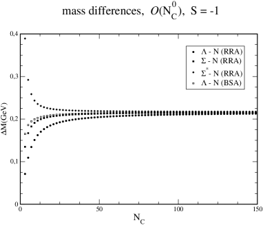
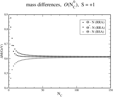
Figure 3: Mass differences at ${\cal O}(N_{C}^{0})$ computed for $\epsilon=4.25$ in the Skyrme model as functions of $N_{C}$. In the RRA they are the corresponding differences of the eigenvalues in eq. (61) while in the BSA they are extracted from eq. (42). Left panel $\Delta S=-1$; right panel $\Delta S=+1$.

As $N_{C}\to\infty$ the BSA for fluctuations in the rotational subspace predicts $\omega_{\Lambda}$ and $\omega_{\Theta}$ for those mass differences regardless of spin and isospin. Obviously this is matched by the RRA. In figure 4 we display the mass differences that scale like ${\cal O}(1/N_{C})$, i.e. we compute the hyperfine splitting in both approaches. In doing so we only consider combinations for which in the BSA the ordering ambiguities and omissions from ${\cal O}(\eta_{\alpha}^{4})$ terms cancels, i.e. baryons with identical strangeness.

                 

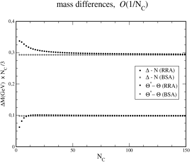
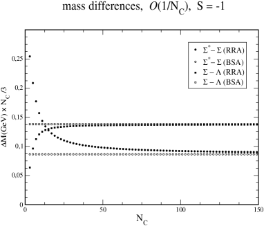
Figure 4: Mass differences at ${\cal O}(1/N_{C})$ computed for $\epsilon=4.25$ in the Skyrme model as functions of $N_{C}$. Left panel: baryons with strangeness $S=0,1$; right panel $S=-1$. See also caption of figure 3.

Again, perfect agreement between the two approaches is observed for $N_{C}\to\infty$. However, at $N_{C}=3$ sizable $1/N_{C}$ corrections occur that cannot be accounted for by the BSA.

A couple of further comments are in order. First, when computing matrix elements we observe that, cf. eq. (58),

$$\frac{\Gamma}{2}\big{\langle}1-D_{88}\big{\rangle}={\cal O}(N_{C}^{0})\,,$$ (62)

that is, the net effect of flavor symmetry breaking in the RRA is an ${\cal O}(N_{C}^{0})$ contribution to the baryon mass. Again, this is consistent with the BSA where flavor symmetry breaking enters the ${\cal O}(N_{C}^{0})$ equation of motion for the kaon fluctuations (20). Second, the literature contains claims that the $\Delta$–nucleon mass difference would scale like ${\cal O}(N_{C}^{0})$ once symmetry breaking is incorporated in the RRA Pr03 . The actual calculation, displayed in fig 4, shows that this is not correct. As in two extreme cases, zero and infinite symmetry breaking, this mass difference scales like ${\cal O}(1/N_{C})$. The physical value, $m_{K}=495{\rm MeV}$ is intermediate to these extreme cases and it thus comes to no surprise that this mass difference vanishes as $N_{C}\to\infty$.

The second remark concerns the eventual restriction of collective coordinates to only dynamical zero modes. For zero symmetry breaking ($\Gamma=0$) the rigid rotation eigenstates of eq.(61) are states in the $\mathbf{8}$, $\mathbf{10}$, $\overline{\mathbf{10}}$, $\mathbf{27}$,… dimensional representations of flavor $SU(3)$. Though the anti–kaon fluctuations are zero frequency solutions in the BSA, the kaon fluctuations are not due to the Wess–Zumino term, i.e. the latter are not really dynamical zero–modes. Therefore it has been suggested to introduce collective coordinates only for the anti–kaonic zero–modes in a manner that only the octet and decuplet would be treated collectively Ch05 . Such an approach seems complicated because constraints on both the fluctuations and the collective coordinates are required. Putting the question of feasibility aside, there is no advantage in doing so to study the $\Theta^{+}$ pentaquark since such a treatment essentially corresponds to the BSA and prevents the incorporation of finite $N_{C}$ effects. The restriction to the octet and decuplet seems even more problematic in view of flavor symmetry breaking ($\Gamma\neq 0$) as it mixes baryon states from different $SU(3)$ representations Pa89a . In particular the nucleon wave–function contains admixture of the nucleon type state in the $\overline{\mathbf{10}}$. Thus the latter may not be omitted.

To round up this section on the RRA we note that other approaches to quantize chiral solitons in flavor $SU(3)$, like the slow rotator Schw92 or the breathing mode Sch91a approaches, are essentially extensions of the RRA.

So far we have established the relation between rotational excitations of the soliton and the bound states in the large–$N_{C}$ limit. In order to study the decay width of the $\Theta^{+}$ pentaquark we need to introduce fluctuations by extending the RRA to the RVA.

V Collective rotations and vibrations

We will now include the kaon fluctuations in the RVA according to the ansatz (11) and compare it to results for the fluctuations in the BSA, section III. The flavor rotating hedgehog $A_{3}(t)U_{0}(\vec{x\,})A^{\dagger}_{3}(t)$ is not a solution to the field equations. Hence the expansion of the action with respect to $\widetilde{\eta}$ has a linear term. This linear term gives rise to Yukawa couplings like $KN\Lambda$ and $KN\Theta$. As a consequence the $KN$ phase shift in the isospin $I=0$ channel has contributions from (iterated) exchange of $\Lambda$ and $\Theta$. Technically, these exchange contributions emerge in the equation of motion for $\widetilde{\eta}$ as a separable potential of the form ”(Yukawa interaction)$\times$(propagator)$\times$(Yukawa interaction)”. The reader may want to peak ahead to eq. (79) for the explicit expression. We have already noted that the background field $\overline{\eta}$, that we have computed in section III, obeys an equation of motion that is obtained from the one for $\widetilde{\eta}$ by omitting the Yukawa couplings. That is, the respective equations of motion differ by this separable potential and we can straightforwardly construct $\widetilde{\eta}$ from $\overline{\eta}$ using standard Lippmann–Schwinger equation techniques. This will make the role of exchanged resonances very transparent. For convenience we list the notation for the involved radial functions

$$\begin{array}[b]{ll}\eta(r):&\mbox{\rm solution to eq.~{}(\ref{scndorder}) in the BSA}\cr\overline{\eta}(r):&\mbox{\rm solution to the integro--differential equation,~{}(\ref{intdiff}) with constraints}\cr\widetilde{\eta}(r):&\mbox{\rm solution to the integro--differential equation,~{}(\ref{Yukawa1}) with constraints and Yukawa exchange}\end{array}$$

We will establish two central results in the large–$N_{C}$ limit:

• We compute the RVA fluctuations $\widetilde{\eta}$ by supplementing the equations of motion for $\overline{\eta}$ with the effects due to $\Lambda$ and $\Theta$ exchanges. We compute the phase shifts for $\widetilde{\eta}$ and show that they are identical to those computed from $\eta$ in the BSA, eq. (10).

• We separate the Yukawa exchange contributions to the scattering amplitude and find the corresponding phase shift to equal the resonance phase shift displayed in figure 2.

In doing so we need to identify the Yukawa couplings by computing the terms linear in $\widetilde{\eta}$. Note that in the action all linear terms must occur as iso–singlets. Then there are two sources for Yukawa terms: 1) the flavor symmetric piece $\Gamma_{SK}+\Gamma_{WZ}$ has couplings to the angular velocities $\Omega_{a}$, 2) the symmetry breaking piece has a contraction between $D_{8a}$ and $\widetilde{\eta}_{a}$. For the moment we will only consider the first case and relegate the discussion of flavor symmetry breaking to section VII.

In the flavor symmetric case there are already many rotation–vibration coupling terms linear and quadratic in $\Omega_{a}$. In order to keep the calculation feasible we keep only those terms that survive in the large–$N_{C}$ limit. The so–selected Yukawa coupling is then treated to all orders in $N_{C}$. Admittedly, this procedure is not completely consistent and the neglected couplings are not necessarily small at $N_{C}=3$. However, a major purpose of the present investigation is to show the equivalence with the BSA. For this purpose it completely suffices to only consider the leading $N_{C}$ couplings. In order to isolate these terms we need to discuss the $N_{C}$ scaling of the angular velocities $\Omega_{a}$ to identify those Yukawa terms that survive in the large–$N_{C}$ limit. That is straightforward for $a=1,\ldots,7$ as we simply invert eq. (46),

$$\sum_{i=1}^{3}\Omega_{i}^{2} = \frac{J(J+1)}{\Theta_{\pi}^{2}}\quad{\Rightarrow}\quad\Omega_{i}={\cal O}\left(1/N_{C}\right)\quad\mbox{\it i.e.\@}\quad R_{i}={\cal O}(N_{C}^{0})\,,$$ (63)

$$\sum_{\alpha=4}^{7}\Omega_{\alpha}^{2} = \frac{C_{2}-J(J+1)-N_{C}^{2}/12}{\Theta_{K}^{2}}\quad{\Rightarrow}\quad\Omega_{\alpha}={\cal O}\left(1/\sqrt{N_{C}}\right)\quad\mbox{\it i.e.\@}\quad R_{\alpha}={\cal O}(\sqrt{N_{C}})\,,$$ (65)

as the moments of inertia $\Theta_{\pi}$ and $\Theta_{K}$ are ${\cal O}\left(N_{C}\right)$. In the large–$N_{C}$ expansion $\Omega_{i}$ ($i=1,2,3$) is thus subleading to $\Omega_{\alpha}$ ($\alpha=4,\ldots,7$) and may be omitted. As shown in the appendix, the angular velocity $\Omega_{8}$ may be absorbed in a suitable redefinition of the energy scale

$$\omega\longrightarrow\omega+\frac{\sqrt{3}}{2}\Omega_{8}\,,$$ (66)

where $\omega$ is the frequency of the kaon fluctuation, cf. eq. (13). Thus, to compute the $\Omega$–$\widetilde{\eta}$ Yukawa coupling we only need to consider the kaonic angular velocities $\Omega_{\alpha}=-R_{\alpha}/\Theta_{K}$ with $\alpha=4,\ldots,7$. This lengthy calculation described in the appendix not only requires to extract the terms in the action that are linear in $\widetilde{\eta}$ but also to consider the constraints, eq. (27) because they contain pieces that are of the same linear order in $\widetilde{\eta}$. Having extracted these linear terms we are unfortunately not yet in the position to compute matrix elements of the interaction Hamiltonian (69) between $\Theta$ and $KN$ states in the space of the collective coordinates. The reason is that $\widetilde{\eta}$ parameterizes the kaon field in the intrinsic frame. A collective flavor rotation relates the intrinsic fluctuations to those in the laboratory frame, that are observed in kaon–nucleon scattering,

$$\widetilde{\xi}_{a}=D_{ab}\widetilde{\eta}_{b}\,,$$ (67)

with $a,b=1,\ldots,8$. In the large–$N_{C}$ limit, $D_{\alpha i}$ and $D_{\alpha 8}$, the couplings to the intrinsic pions and $\eta$, respectively, are suppressed. Hence we approximate

$$\widetilde{\xi}_{\alpha}=D_{\alpha\beta}\widetilde{\eta}_{\beta}\,,$$ (68)

with $\alpha,\beta=4,\ldots,7$. Finally the resulting interaction Hamiltonian reads,

$$H_{\rm int}=\frac{2f_{\pi}}{\Theta_{K}}\,d_{i\alpha\beta}\,D_{\gamma\alpha}R_{\beta}\,\int d^{3}r\,{\rm sin}\frac{F(r)}{2}\left[2\lambda(r)-\omega_{0}M_{K}(r)\right]\hat{x}_{i}\widetilde{\xi}_{\gamma}(\vec{x\,},t)R_{\beta}\,,$$ (69)

where $d_{i\alpha\beta}$ are the symmetric structure constants of $SU(3)$. The pieces involving $\omega_{0}=N_{C}/4\Theta_{K}$ and $\lambda(r)$ stem from $\Gamma_{SK}$ and $\Gamma_{WZ}$, respectively. From eqs. (7), (65) we easily verify that $H_{\rm int}={\cal O}(N_{C}^{0})$.

We need to compute matrix elements of the interaction Hamiltonian, eq. (69) between a kaon nucleon state coupled to good spin ($J$) and isospin ($I$) and a collective excitation with the same quantum numbers. We denote the operator that annihilates a kaon in the laboratory frame with isospin projection $i=\pm\mbox{\small$\frac{1}{2}$}$ and orbital angular momentum ($\ell,m$) by $a^{(i)}_{\ell,m}$ and use the Wigner–Eckart theorem to reduce the matrix elements of $H_{\rm int}$ to those computed in the space of the collective coordinates,

$$\sum_{i=\pm\frac{1}{2}}\langle\Theta|a^{(i)}_{1,m}d_{m\alpha\beta}D_{\gamma(i)\alpha}R_{\beta}|(KN)_{I=0,J=\frac{1}{2}}\rangle=\sqrt{6}\,\langle\Theta^{+}\uparrow|d_{3\alpha\beta}D_{+\alpha}R_{\beta}|n\uparrow\rangle$$ (70)

where $\gamma(\pm\mbox{\small$\frac{1}{2}$})$ maps the isospin projection onto the flavor indices, $D_{\pm a}=D_{4a}\pm iD_{5a}$. The arrow indicates the spin projection $J_{3}=\mbox{\small$\frac{1}{2}$}$. In what follows we will always adopt this value without explicit mention. Orbital angular momentum $\ell=1$ is projected onto by $\hat{x}_{i}$ in $H_{\rm int}$. Of course, that is nothing but the statement that only the P–wave channel is affected by the rigid rotations. A similar reduction formula holds for the matrix element of $H_{\rm int}$ between final $\Lambda$ and initial anti–kaon nucleon states. In the flavor symmetric case the relevant matrix elements of the collective coordinate operators are

$$\langle\Theta^{+}|d_{3\alpha\beta}D_{+\alpha}R_{\beta}|n\rangle = \frac{N_{C}+1}{4}\sqrt{\frac{N_{C}+1}{2\left(N_{C}+3\right)\left(N_{C}+7\right)}}=:X_{\Theta}\sqrt{\frac{N_{C}}{32}}$$ (71)

$$\langle\Lambda|d_{3\alpha\beta}D_{-\alpha}R_{\beta}|p\rangle = -\frac{1}{2}\frac{N_{C}+5}{\left(N_{C}+7\right)\sqrt{2N_{C}+6}}=:X_{\Lambda}\sqrt{\frac{N_{C}}{32}}\,.$$ (73)

For the matrix elements in eq. (73) we have factored the large–$N_{C}$ value for later convenience

$$X_{\Theta} = \sqrt{\frac{\left(N_{C}+1\right)^{3}}{N_{C}\left(N_{C}+3\right)\left(N_{C}+7\right)}}=\begin{cases}1\,,&\quad N_{C}\to\infty\cr\frac{4}{3\sqrt{5}}\,,&\quad N_{C}=3\end{cases}$$ (74)

$$X_{\Lambda} = -\frac{2\left(N_{C}+5\right)}{\left(N_{C}+7\right)\sqrt{N_{C}\left(N_{C}+3\right)}}=\begin{cases}0\,,&\quad N_{C}\to\infty\cr-\frac{4\sqrt{2}}{15}\,,&\quad N_{C}=3\end{cases}\,.$$ (76)

Only the $\Theta^{+}$ Yukawa coupling survives as $N_{C}\to\infty$. Hence there is only one intermediate state in that limit. For the physical value, $N_{C}=3$, the collective coordinate part of the $\Lambda$ Yukawa coupling constant is actually larger in magnitude than that of $\Theta^{+}$.

Obviously this explicit derivation of the interaction Hamiltonian yields only a single $SU(3)$ structure (i.e. $d_{i\alpha\beta}\hat{x}_{i}D_{a\alpha}R_{\beta}$) for the $\Theta-N$ transition. This is to be contrasted with earlier studies Di97 ; Pr03 ; El04 ; Pr05 who ”invented” three structures, even in the flavor symmetric case.

We want to add the particle exchanges induced by $H_{\rm int}$ to the differential equation, (34) for the constrained fluctuations, $\overline{\eta}$ (still omitting symmetry breaking). The propagators are $(\omega_{\Theta}-\omega)^{-1}$ and $(\omega_{\Lambda}+\omega)^{-1}$ for $\Theta$ and $\Lambda$, respectively, because the differential equations for kaons and anti–kaons are related by $\omega\leftrightarrow-\omega$. Thus the Yukawa terms induce the separable potential

$$\frac{\left|\langle\Theta|H_{\rm int}|(KN)_{I=0}\rangle\right|^{2}}{\omega_{\Theta}-\omega}+\frac{\left|\langle\Lambda|H_{\rm int}|(KN)_{I=0}\rangle\right|^{2}}{\omega_{\Lambda}+\omega}\,.$$ (77)

Note that these matrix elements concern the $T$–matrix elements in the laboratory frame. However, we observe from eq. (12) that for the $\Theta^{+}$ channel the laboratory and intrinsic $T$–matrix elements are identical. Hence we may add the exchange potential, eq. (77) in the intrinsic frame. We then end up with the modified integro–differential equation

$$h^{2}\widetilde{\eta}(r)+\omega\left[2\lambda(r)-\omega M_{K}(r)\right]\widetilde{\eta}(r)=-z(r)\left[\int_{0}^{\infty}r^{\prime 2}dr^{\prime}z(r^{\prime})2\lambda(r^{\prime})\widetilde{\eta}(r^{\prime})\right]$$ (78)

$$\hskip 56.9055pt\times\left[2\lambda(r)-\left(\omega+\omega_{0}\right)M_{K}(r)-\omega_{0}\left(\frac{X_{\Theta}^{2}}{\omega_{\Theta}-\omega}+\frac{X_{\Lambda}^{2}}{\omega}\right)\left(2\lambda(r)-\omega_{0}M_{K}(r)\right)\right]\,,\hskip 28.45274pt$$ (79)

in the flavor symmetric case. The particular coefficient, $\omega_{0}$ of the Yukawa contribution will become clear when we discuss the width of $\Theta^{+}$ in the next section. The Yukawa contribution to the integro–differential equation is orthogonal to the zero–mode,

$$\int_{0}^{\infty}r^{2}dr\,z(r)\left[2\lambda(r)-\omega_{0}M_{K}(r)\right]z(r)=0$$ (80)

and thus any solution to eq. (79) still satisfies the second constraint in eq. (27) which we subsequently employ to simplify the integral.

The essential observation is that eq. (79) has a simple solution as $N_{C}\to\infty$ ($X_{\Theta}=1$ and $X_{\Lambda}=0$)

$$\widetilde{\eta}(r)=\eta(r)-az(r)\qquad{\rm with}\qquad a=\int_{0}^{\infty}drr^{2}\,z(r)M_{K}(r)\eta(r)\,.$$ (81)

Here $\eta(r)$ is the solution to the unconstrained equation (20) in the BSA. The radial function, $z(r)$ associated with the zero–mode is localized in space. Thus the phase shifts of $\eta$ and $\widetilde{\eta}$, which are extracted from the respective asymptotic behaviors are identical. This proves our assertion A). In turn this shows that the difference of the phase shifts defined in eq. (35) is directly related to the resonance exchange. This proves our assertion B). In section VII we will show that these assertions also hold when symmetry breaking is included even though that case is significantly more involved as e.g. $\lim_{N_{C}\to\infty}X_{\Lambda}\neq 0$.

VI The width of the $\Theta^{+}$

In this section we will show that the Yukawa terms can be imposed to compute the width of the exchanged particles. For simplicity we will still omit flavor symmetry breaking.

VI.1 Large–$N_{C}$ limit

In a first step we show that in the large–$N_{C}$ limit the iterated exchange, that is induced by the Yukawa terms in eq. (79), leads to the resonance phase shift discussed already in section IV. That is, we want to prove assertion B) by showing that the resonance width associated with $\delta_{R}(k)$ equals that induced by the Yukawa coupling of $\Theta^{+}$.

For large–$N_{C}$ we may omit the $\Lambda$–exchange. Then the reaction matrix formalism is most suitable to compute $\delta_{R}(k)$ from the iterated exchange of a single resonance. The (real) reaction matrix obeys the Lippmann–Schwinger equation

$$R=V+V\overline{G}_{0}R\,,$$ (82)

where $\overline{G}_{0}$ and $V$ are the Green’s function for the constrained problem, eq. (34) and the separable potential due to the particle exchange, eq. (77), respectively. We stress that this is an exact solution to the scattering problem rather than any type of Born or distorted wave Born approximation. The solution to the Lippmann–Schwinger equation is most conveniently obtained in a basis independent formal language

$$\overline{G}_{0}(\omega) = \frac{1}{\pi\omega}\,{\cal P}\,\int_{0}^{\infty}q^{2}dq\,\left[\frac{|\overline{\eta}_{\omega_{q}}\rangle\langle\overline{\eta}_{\omega_{q}}|}{\omega-\omega_{q}}+\frac{|\overline{\eta}_{-\omega_{q}}\rangle\langle\overline{\eta}_{-\omega_{q}}|}{\omega+\omega_{q}}\right]$$ (83)

$$V(\omega) = -\frac{\omega_{0}}{\omega_{\Theta}-\omega}|g_{\Theta}\rangle\langle g_{\Theta}|\qquad{\rm with}\qquad\langle r|g_{\Theta}\rangle=X_{\Theta}\left(2\lambda(r)-\omega_{0}M_{K}(r)\right)z(r)\,,$$ (85)

where $\omega_{p}=\sqrt{p^{2}+m_{K}^{2}}$ and ${\cal P}$ denotes the principle value prescription. In the above expression $\overline{\eta}$ appears, rather than $\widetilde{\eta}$, because the interaction Hamiltonian is treated as an additional interaction for the constrained fluctuations and we thus require the Green’s function for $\overline{\eta}$. The potential is obtained from eq. (77) by setting $X_{\Lambda}=0$. We find the reaction matrix

$$R=\frac{\omega_{0}X_{\Theta}^{2}|\left(2\lambda-\omega_{0}M_{K}\right)z\rangle\langle z\left(2\lambda-\omega_{0}M_{K}\right)|}{\omega-\omega_{\Theta}-\omega_{0}\langle z(2\lambda)|\overline{G}_{0}(\omega)|(2\lambda)z\rangle}$$ (86)

since $\langle\overline{\eta}_{\omega}|M_{K}z\rangle=0$. The resonance phase shift induced by $V$ is obtained from the diagonal matrix element of the R–matrix, $k\langle\overline{\eta}_{\omega_{k}}|R|\overline{\eta}_{\omega_{k}}\rangle=-{\rm tan}\left(\delta_{\rm R}(k)\right)$, yielding

$${\rm tan}\left(\delta_{\rm R}(k)\right)=\frac{\Gamma(\omega_{k})/2}{\omega_{\Theta}-\omega_{k}+\Delta(\omega_{k})}\,.$$ (87)

This phase shift exhibits the canonical resonance structure with the width

$$\Gamma(\omega_{k})=2k\omega_{0}X_{\Theta}^{2}\left|\int_{0}^{\infty}r^{2}dr\,z(r)2\lambda(r)\overline{\eta}_{\omega_{k}}(r)\right|^{2}$$ (88)

and the pole shift

$$\Delta(\omega_{k})=\frac{1}{2\pi\omega_{k}}\,{\cal P}\,\int_{0}^{\infty}qdq\,\left[\frac{\Gamma(\omega_{q})}{\omega_{k}-\omega_{q}}+\frac{\Gamma(-\omega_{q})}{\omega_{k}+\omega_{q}}\right]\,.$$ (89)

Of course, we have numerically verified that in the large–$N_{C}$ limit with $X_{\Theta}^{2}=1$, the phase shift from eq. (87) is identical to the one that we calculated as the difference in eq. (35). For finite $N_{C}$ the width $\Gamma$ acquires a factor $X_{\Theta}^{2}\neq 1$ and the R–matrix formalism becomes two–dimensional ($\Lambda$ and $\Theta^{+}$ exchange).

We stress that although the singularity of the scattering amplitude is shifted by the amount $\Delta$ due to iterated resonance exchange, the ”bare” mass of the resonance is $\omega_{\Theta}$, the pentaquark mass predicted in the RRA.

Alternatively we have applied Fermi’s golden rule to compute the transition rate $\Theta\to KN$ from the interaction Hamiltonian, eq. (69). This leads identically to the result displayed in eq. (88) and shows that the way we have included the separable potential in eq. (79) is unique.

Figure 5: The resonance phase shift as a function of $N_{C}$ for $m_{K}=m_{\pi}$.

VI.2 Finite $N_{C}$

As already mentioned, the R–matrix formalism is two dimensional at finite $N_{C}$ because the $\Lambda$ exchange cannot be omitted. It is therefore more convenient to compute the resonance phase shift in a fashion similar to eq. (35). First we compute the phase shift with both Yukawa interactions included from $\widetilde{\eta}$ in eq. (79). From that we get the resonance phase shift by subtracting the background phase shift that we extract from $\overline{\eta}$ in eq. (34). The resulting resonance phase shifts in the $\Theta^{+}$ channel are displayed in figure 5. It is illuminating to see how the BSA result emerges in the limit $N_{C}\to\infty$. Obviously this resonance becomes sharper and the pole shift decreases (in magnitude) to $\Delta=-14{\rm MeV}$ as the number of color assumes its physical value $N_{C}=3$. This is mainly due to the reduction of $X_{\Theta}$. Furthermore, at finite $N_{C}$ the bare resonance position is increased to $\omega_{\Theta}=(N_{C}+3)/4\Theta_{K}$, according to eq. (60). This $N_{C}$–dependence of the resonance position is clearly exhibited in figure 5.

There are two competing effects on the width when approaching the physical value, $N_{C}=3$. The position of the pole is increased by about a factor of two. This increases the available phase space and thus the width. On the other hand, the collective coordinate matrix element $X_{\Theta}^{2}$ decreases by approximately a factor 3, cf. eq. (76). According to eq. (88) this decreases the width.

At this point it is also illuminating to consider the large–$N_{C}$ expansion of these matrix elements in more detail. For example

$$X_{\Theta}^{2}\,\longrightarrow\,1-\frac{7}{N_{C}}+\frac{52}{N_{C}^{2}}-\frac{372}{N_{C}^{3}}+\frac{2628}{N_{C}^{4}}+\ldots\,\,,$$ (90)

does not converge for $N_{C}\leq 7$. This clearly demonstrates that taking only leading pieces from a large–$N_{C}$ expansion of these matrix elements yields incorrect results for $N_{C}=3$. It is unavoidable to include finite $N_{C}$ effects. Any approach Je04 that employs $1/N_{C}$ expansion methods for exotic baryon matrix elements at $N_{C}=3$ seems questionable.

VI.3 Comparison with other approaches to compute the width

We stress that the appearance of only a single rather than two $SU(3)$ structures in the transition Hamiltonian in the flavor symmetric limit is not an artifact in the (eventually oversimplified) Skyrme model whose action is a functional of only pseudoscalar mesons. Rather it generalizes to all chiral soliton models. The reason is simple. Starting point in all these models is the introduction of intrinsic fluctuations about the classical soliton, i.e. the generalization of the ansatz, eq. (11) to parameterize additional fields. In this intrinsic formulation the interaction Hamiltonian must be an isoscalar operator that is linear in kaonic fluctuations and projects onto the P–wave channel. At ${\cal O}(N_{C}^{0})$ only $d_{i\alpha\beta}\hat{x}_{i}\widetilde{\eta}_{\alpha}\Omega_{\beta}$ is possible. Of course, in more extended models $\widetilde{\eta}_{\alpha}$ also involves other strange degrees of freedom, e.g. $K^{*}$. In the flavor symmetric formulation the adjoint representation of the collective coordinates, $D_{ab}$, emerges only by the transformation to the laboratory system as in eq. (67). To see whether or not the limitation to only a single $SU(3)$ structure in the transition Hamiltonian is an artifact of the Skyrme model it is instructive to recall how the authors of refs. Di97 ; El04 came to the improper use of several $SU(3)$ structures regardless of flavor symmetry breaking. Starting point of those studies is the spatial part of the axial current and its identification with the kaon field operator via PCAC. This axial current is commonly computed from the rigidly rotating classical field only and in general allows for three $SU(3)$ structures in the flavor symmetric case. One of those structures is directly related to the presumably small singlet current matrix element and is usually ignored in the context of the $\Theta^{+}$ width. In the simple Skyrme model it vanishes exactly. However, the other two structures are also present in the Skyrme model axial current Ka87 . They simply do not show up in the transition Hamiltonian. Stated otherwise, the axial current operator is not suitable to compute hadronic decay widths in chiral soliton models. A simple reason is that the isospin embedding of the hedgehog soliton, eq. (8) breaks flavor symmetry. In particular this prevents using $SU(3)$ to relate various hadron decay widths among each other. For example, the computation of the $\Delta\to\pi N$ width requires a term linear in the intrinsic pion fluctuations which involves collective coordinate operators that are not related to $d_{i\alpha\beta}\hat{x}_{i}\widetilde{\eta}_{\alpha}\Omega_{\beta}$.

Of course, in our approach $\partial^{\mu}A_{\mu}^{a}=f_{\pi}m_{a}^{2}\phi^{a}+{\cal O}(\phi^{3})$, i.e. PCAC, holds as well. It is nothing but the equation of motion for the chiral angle and the meson fluctuations that we solve. That is, in our approach PCAC is satisfied at ${\cal O}(N_{C})$ and ${\cal O}(N_{C}^{0})$ while in refs. Di97 ; El04 the equation of motion is only considered at ${\cal O}(N_{C})$. The main point, however, is that within soliton models the right hand side may not be the interpolating field for the pseudoscalar meson in the final state of hadronic decays.

VII SU(3) symmetry breaking

In section V we have established the equivalence of the bound state and rotation–vibration coupling approaches for computing the kaon nucleon phase shift in the large–$N_{C}$ limit in the flavor symmetric case. Here we will extend that discussion to the symmetry breaking case.

The interaction Hamiltonian that describes the Yukawa exchange for fluctuations in the laboratory frame, cf. eq. (69), acquires an additional term from the symmetry breaking part of the action, $\Gamma_{\rm SB}$,

$$H_{\rm int} = \frac{2f_{\pi}}{\Theta_{K}}d_{i\alpha\beta}D_{\gamma\alpha}R_{\beta}\int d^{3}r\,{\rm sin}\frac{F(r)}{2}\left[2\lambda(r)-\omega_{0}M_{K}(r)\right]\widetilde{\xi}_{\gamma}(\vec{x\,},t)\hat{x}_{i}$$ (93)

$$\hskip 14.22636pt-\frac{4f_{\pi}}{\sqrt{3}}d_{i\alpha\beta}D_{\gamma\alpha}D_{8\beta}\int d^{3}r\,{\rm sin}\frac{F(r)}{2}\left[m_{K}^{2}-m_{\pi}^{2}-\frac{3\Gamma}{8\Theta_{K}}M_{K}(r)\right]\widetilde{\xi}_{\gamma}(\vec{x\,},t)\hat{x}_{i}\,.$$

We provide the detailed derivation of this interaction Hamiltonian in the appendix. In principle, there are many pole contributions, such as from states with $S=\pm 1$ and $I=0$ that stem from higher dimensional $SU(3)$ representations. They lead to sharp resonances at higher energies and may be omitted for the energy regime of current interest. We thus keep only the contributions associated with the exchanges of $\Lambda$ and $\Theta^{+}$. Then the separable Yukawa exchange potential in the P–wave has the general form

$$V(\omega) = -\frac{\omega_{0}}{\omega_{\Theta}-\omega}|g_{\Theta}\rangle\langle g_{\Theta}|-\frac{\omega_{0}}{\omega_{\Lambda}+\omega}|g_{\Lambda}\rangle\langle g_{\Lambda}|$$ (94)

$$\langle r|g_{\nu}\rangle = X_{\nu}\left(2\lambda(r)-\omega_{0}M_{K}(r)\right)z(r)+\frac{Y_{\nu}}{\omega_{0}}\left(m_{K}^{2}-m_{\pi}^{2}-\frac{3\Gamma}{8\Theta_{K}}M_{K}(r)\right)z(r)\,,\quad\nu=\Theta,\Lambda\,.\qquad$$ (96)

Note that $\langle z|g_{\nu}\rangle=0$. This implies that the solutions to the constrained equation of motion (34) with this potential added, also do satisfy the constraint $\langle z|M_{K}\widetilde{\eta}\,\rangle=0$.

The matrix elements $X_{\nu}$ have already been defined in eq. (73). Similarly we introduce

$$\langle\Theta^{+}|d_{3\alpha\beta}D_{+\alpha}D_{8\beta}|n\rangle =: Y_{\Theta}\sqrt{\frac{3}{8N_{C}}}$$ (97)

$$\langle\Lambda|d_{3\alpha\beta}D_{-\alpha}D_{8\beta}|p\rangle =: Y_{\Lambda}\sqrt{\frac{3}{8N_{C}}}\,,$$ (99)

where $Y_{\Theta}$ and $Y_{\Lambda}$ tend to unity in the flavor symmetric case as $N_{C}\to\infty$. Of course, for non–zero symmetry breaking the matrix elements $X_{\nu}$ and $Y_{\nu}$ have to be computed numerically and cannot be given as simple functions of $N_{C}$, results are listed in table 1.

The integro–differential equation with the Yukawa pieces included is a bit more complicated than in the flavor symmetric case, eq. (79),

$$h^{2}\widetilde{\eta}+\omega\left(2\lambda-\omega M_{K}\right)\widetilde{\eta} =$$ (108)

$$-\Big{[}2\lambda-\left(\omega+\omega_{0}\right)M_{K}-\omega_{0}\left(\frac{X_{\Theta}^{2}}{\omega_{\Theta}-\omega}+\frac{X_{\Lambda}^{2}}{\omega_{\Lambda}+\omega}\right)\left(2\lambda-\omega_{0}M_{K}\right)$$

$$-\left(\frac{X_{\Theta}Y_{\Theta}}{\omega_{\Theta}-\omega}+\frac{X_{\Lambda}Y_{\Lambda}}{\omega_{\Lambda}+\omega}\right)\left(m_{K}^{2}-m_{\pi}^{2}-\frac{3\Gamma}{8\Theta_{K}}M_{K}\right)\Big{]}z\int_{0}^{\infty}drr^{2}z(2\lambda)\widetilde{\eta}$$

$$+\left(m_{K}^{2}-m_{\pi}^{2}\right)\Big{[}M_{K}+\left(\frac{X_{\Theta}Y_{\Theta}}{\omega_{\Theta}-\omega}+\frac{X_{\Lambda}Y_{\Lambda}}{\omega_{\Lambda}+\omega}\right)\left(2\lambda-\omega_{0}M_{K}\right)$$

$$+\frac{1}{\omega_{0}}\left(\frac{Y_{\Theta}^{2}}{\omega_{\Theta}-\omega}+\frac{Y_{\Lambda}^{2}}{\omega_{\Lambda}+\omega}\right)\left(m_{K}^{2}-m_{\pi}^{2}-\frac{3\Gamma}{8\Theta_{K}}M_{K}\right)\Big{]}z\int_{0}^{\infty}drr^{2}z\widetilde{\eta}\,.$$

For simplicity we have omitted the arguments of the radial functions.

Let $\eta(r)$ again be a solution to the BSA equation (20). In the limit $N_{C}\to\infty$ we require that $\widetilde{\eta}=\eta-az$ with $a=\int_{0}^{\infty}drr^{2}\,z(r)M_{K}(r)\eta(r)$ is a solution to eq. (108) also in the case that symmetry breaking ($m_{K}\neq m_{\pi}$) is included. Modulo phase conventions this implies

$$X_{\Theta}=\frac{\omega_{\Theta}}{\omega_{0}}Y_{\Theta}\,,\qquad X_{\Lambda}=-\frac{\omega_{\Lambda}}{\omega_{0}}Y_{\Lambda}\,,\qquad Y_{\Theta}=Y_{\Lambda}=\sqrt{\frac{\omega_{0}}{\omega_{\Theta}+\omega_{\Lambda}}}\,,$$ (109)

as $N_{C}\to\infty$. And indeed, the matrix elements in eqs. (73) and (99) give these results when computed with the exact solutions to eigenvalue equation (61) with flavor symmetry breaking included! In table 1 we display numerical results for these matrix elements for the physical case $N_{C}=3$ and the large–$N_{C}$ limit for various values of $m_{K}$. The third entry, $m_{K}=750{\rm MeV}$ yields the value of the symmetry breaking parameter $\Gamma$ that we would have obtained if we had included symmetry breaking terms that contain derivatives of the chiral field. Obviously, there are significant deviations from the large–$N_{C}$ limit at $N_{C}=3$.

$N_{C}$ $X_{\Theta}$ $Y_{\Theta}$ $X_{\Lambda}$ $Y_{\Lambda}$ $X_{\Theta^{*}}$ $Y_{\Theta^{*}}$ $m_{K}=m_{\pi}$ $3$   0.596   0.149   -0.377   0.189   0.257   0.138 $\infty$ 1 1 0 1 0.667 0.667 $m_{K}=495{\rm MeV}$ 3 0.690 0.168 -0.427 0.195 0.307 0.142 $\infty$ 1.069 0.691 -0.378 0.691 0.713 0.461 $m_{K}=750{\rm MeV}$ 3 0.801 0.188 -0.497 0.203 0.376 0.147 $\infty$ 1.157 0.575 -0.582 0.575 0.771 0.383

Table 1: Matrix elements of collective coordinate operators for $N_{C}=3$ and $N_{C}\to\infty$ and various values of $m_{K}$, cf. eqs. (73), (99) and (117). The third entry, $m_{K}=750{\rm MeV}$ is chosen such as to compensate for the omitted derivative type symmetry breaker.

The large–$N_{C}$ equation of motion for $\widetilde{\eta}$ has a bound state solution in the anti–kaon channel exactly at the BSA energy $\omega_{\Lambda}=196{\rm MeV}$ (for $m_{K}=495{\rm MeV}$). This is a starting point to discuss corrections to the RRA spectrum caused by the rotation–vibration coupling for finite $N_{C}$ which improves on earlier attempts that introduced fluctuations induced by the rigid rotations We90 . However, that discussion is beyond the scope of this paper.

VIII Soliton model predictions for $\mathbf{\Theta^{+}}$

We have already noted that in the flavor symmetric case the excitation energy of $\Theta^{+}$ is altered according to eq. (60) for finite $N_{C}$. The excitation energy of $\Lambda$ remains at zero. For non–zero symmetry breaking the situation is more complicated as both excitation energies depend on the value for $m_{K}$. That is, we need to substitute

$$\omega_{\Lambda}\,\longrightarrow\,E_{\Lambda}-E_{N}\qquad{\rm and}\qquad\omega_{\Theta}\,\longrightarrow\,E_{\Theta}-E_{N}\,,$$ (110)

where $E_{N,\Theta,\Lambda}$ are the solutions to the eigenvalue problem, eq. (61) in the respective channel for a prescribed $N_{C}<\infty$. In addition, we employ the corresponding eigenstates of eq. (61) to evaluate the matrix elements in eqs. (73) and (99) to numerically compute $X_{\Theta},X_{\Lambda},Y_{\Theta}$ and $Y_{\Lambda}$ at any value of $N_{C}$ and $m_{K}$, cf. table 1. We then compute the resonance phase shift as described in section VI B. The results are shown in figure 6.

Figure 6: The resonance phase shift as a function of $N_{C}$ for $m_{K}=495{\rm MeV}$.

Again these phase shifts exhibit a pronounced resonance structure. As in the flavor symmetric case, finite $N_{C}$ effects cause the pole position to move to higher momenta and also the resonance to become sharper. Although the phase shifts displayed in figures 5 and 6 as a function of momentum seem to be similar this is not the case for the resonance energy since it is subject to the dispersion relation $\omega=\sqrt{k^{2}+m_{K}^{2}}$ and $m_{K}$ differs significantly in the two case. From figure 6 we read off a $\Theta$–nucleon mass difference of about $750{\rm MeV}$ which is a bit higher than the empirical value of about $600{\rm MeV}$ if the $\Theta^{+}$ signal around $1540{\rm MeV}$ were indeed established. We remark, however, that the actual prediction for this mass difference is quite model dependent, e.g. we have omitted effects due to $f_{K}\neq f_{\pi}$. Also, the inclusion of other fields like scalar– or vector mesons or chiral quarks will alter the quantitative results.

The width function, $\Gamma(\omega)$ is computed from generalizing eq. (88) to also contain symmetry breaking effects,

$$\Gamma(\omega_{k})=2k\omega_{0}\left|X_{\Theta}\int_{0}^{\infty}r^{2}dr\,z(r)2\lambda(r)\overline{\eta}_{\omega_{k}}(r)+\frac{Y_{\Theta}}{\omega_{0}}\left(m_{K}^{2}-m_{\pi}^{2}\right)\int_{0}^{\infty}r^{2}dr\,z(r)\overline{\eta}_{\omega_{k}}(r)\right|^{2}\,,$$ (111)

which arise from the $\Theta^{+}$ matrix elements of the separable potential, eq. (96). Again, $\overline{\eta}$ rather than $\widetilde{\eta}$ appears in the above expression. Note that contributions of the form $\int drr^{2}z(r)M_{K}(r)\overline{\eta}(r)$ vanish due to the second constraint in eq. (27).

We have already mentioned that chiral soliton models only provide qualitative insight in the baryon mass spectrum. At best, we expect the model predictions for masses of exotic baryons to be reliable at the, say, $100{\rm MeV}$ level. Let us therefore now assume that the $\Theta^{+}$ resonance indeed corresponds to the recently asserted pentaquark of mass $M_{\Theta}=1540{\rm MeV}$ and estimate its width from $\Gamma(\omega)$. First, we have to find the corresponding kaon momentum. This is not without ambiguity because in the soliton picture baryon masses are of higher order in $N_{C}$ than the meson fluctuations and thus considered infinitely heavy. Therefore recoil effects are not necessarily included. This yields $k=340{\rm MeV}$ for the kaon momentum. Of course, a simple calculation using relativistic kinematics incorporates recoil effects and leads to $k=270{\rm MeV}$. For these two momenta we respectively read off widths of $47{\rm MeV}$ and $40{\rm MeV}$ for $m_{K}=495{\rm MeV}$ from figure 7. Fortunately the dependence of $\Gamma(\omega)$ on the effective strength of symmetry breaking seems only moderate in the resonance region. Hence the extracted width is not too sensitive on the uncertainties stemming from the omission of the derivative type symmetry breaker and we finally estimate $\Gamma\approx 40{\rm MeV}$ as the width of the $\Theta^{+}$ pentaquark. Though we do not expect chiral soliton model predictions for the widths to be reliable at the $10{\rm MeV}$ level, we note that this result should be considered a small number as it has to be compared to widths of other hadronic decays of baryon resonances, e.g. $\Gamma(\Delta\to\pi N)\approx 120{\rm MeV}$, empirically.

                 

Figure 7: Model prediction for the width, $\Gamma(\omega)$ of $\Theta^{+}$ (left) and $\Theta^{*+}$ (right) for $N_{C}=3$ as function of the momentum $k=\sqrt{\omega^{2}-m_{K}^{2}}$ for three values of the kaon mass. Note that the two figures have different scales.

Finally let us briefly comment on the width of the $\Theta^{*}$ pentaquark, the $J=\frac{3}{2}$ and $I=1$ partner of $\Theta^{+}$. In large–$N_{C}$ the starting point is again the intrinsic $T$–matrix of the BSA. However, for $\Theta^{*}$ the recoupling between intrinsic laboratory frames is more complicated than eq. (12). There are two intrinsic $T$–matrix elements $T_{{\cal G}\ell}=T_{\frac{1}{2}1}$ and $T_{\frac{3}{2}1}$ with different grand spins which contribute to the scattering in the laboratory frame Ha84 ; Ma88 ,

$$T(P13)=\frac{4}{9}\,T_{\mbox{\small$\frac{1}{2}$},1}+\frac{5}{9}\,T_{\mbox{\small$\frac{3}{2}$},1}\,.$$ (112)

While the collective excitation and thus the relevant phase shift displayed in figures 1 and 2 emerges in the intrinsic ${\cal G}=\frac{1}{2}$ channel, the ${\cal G}=\frac{3}{2}$ contributes only to the background phase shift and is irrelevant for the $\Theta^{*}$ resonance structure. From eq. (112) we notice a factor $\frac{4}{9}$ not present in the corresponding relation for $\Theta^{+}$, eq. (12).

In the notation of the $RRA$ and for $m_{K}=m_{\pi}$ the $\Theta^{*}$ dwells in the $"\mathbf{27}"$–plet of flavor $SU(3)$ for finite $N_{C}$ while for $N_{C}\to\infty$ it becomes degenerate with $\Theta^{+}$. For $N_{C}=3$ the $\Theta^{*}$ pentaquark is expected to be roughly $100{\rm MeV}$ heavier than $\Theta^{+}$ Wa03 ; We04 . The Yukawa interactions of the RVA, eq. (93) now lead to (iterated) $\Theta^{*}$ and $\Sigma^{*}$ exchanges.

The matrix elements relevant to compute the width of $\Theta^{*}$ are reduced via

$$\sum_{i=\pm\frac{1}{2}}\langle\Theta^{*}|a^{(i)}_{1,m}d_{m\alpha\beta}D_{\gamma(i)\alpha}R_{\beta}|(KN)_{I=1,J=\frac{3}{2}}\rangle = \sqrt{3}\,\langle\Theta^{*+}\uparrow|d_{3\alpha\beta}D_{+\alpha}R_{\beta}|n\uparrow\rangle$$ (113)

$$\sum_{i=\pm\frac{1}{2}}\langle\Theta^{*}|a^{(i)}_{1,m}d_{m\alpha\beta}D_{\gamma(i)\alpha}D_{8\beta}|(KN)_{I=1,J=\frac{3}{2}}\rangle = \sqrt{3}\,\langle\Theta^{*+}\uparrow|d_{3\alpha\beta}D_{+\alpha}D_{8\beta}|n\uparrow\rangle\,.$$ (115)

The relative factor $1/\sqrt{2}$ in comparison with eq. (70) is essential so that for $\Theta^{*}$ we have to replace $X_{\Theta}\to X_{\Theta^{*}}$ and $Y_{\Theta}\to Y_{\Theta^{*}}$ in eq. (111) by

$$X_{\Theta^{*}}=\frac{4}{\sqrt{N_{C}}}\,\langle\Theta^{*+}\uparrow|d_{3\alpha\beta}D_{+\alpha}R_{\beta}|n\uparrow\rangle\quad{\rm and}\quad Y_{\Theta^{*}}=2\sqrt{\frac{N_{C}}{3}}\,\langle\Theta^{*+}\uparrow|d_{3\alpha\beta}D_{+\alpha}D_{8\beta}|n\uparrow\rangle\,.$$ (116)

In the flavor symmetric case we find

$$X_{\Theta^{*}}=\frac{2}{3}\left(N_{C}-1\right)\sqrt{\frac{N_{C}+5}{N_{C}(N_{C}+3)(N_{C}+9)}}=\,\frac{2}{3}\,\begin{cases}\frac{2}{9}\sqrt{3}&,\quad N_{C}=3\cr\,\,1&,\quad N_{C}=\infty\cr\end{cases}\,.$$ (117)

Thus, disregarding phase space effects (due to $\Theta^{*}$ lying roughly $100{\rm MeV}$ above $\Theta^{+}$ for $N_{C}=3$), we obtain

$$\Gamma_{\Theta^{*}}=\Gamma_{\Theta}\left(\frac{X_{\Theta^{*}}}{X_{\Theta}}\right)^{2}=\Gamma_{\Theta}\begin{cases}\,\frac{5}{27}&,\quad N_{C}=3\cr\,\frac{4}{9}&,\quad N_{C}=\infty\cr\end{cases}\,.$$ (118)

From eq. (117) we notice that in the large–$N_{C}$ limit the factor $\frac{4}{9}$ that appears in eq. (112) is recovered. This is precisely what is required in order to obtain the BSA result in this limit. We have numerically verified that in the symmetry breaking case

$$\lim_{N_{C}\to\infty}\frac{X_{\Theta^{*}}}{X_{\Theta}}=\lim_{N_{C}\to\infty}\frac{Y_{\Theta^{*}}}{Y_{\Theta}}=\frac{2}{3}$$ (119)

for any value $m_{K}\geq m_{\pi}$ such that $\Gamma_{\Theta^{*}}=\frac{4}{9}\Gamma_{\Theta}$ in that case as well, see also table 1. Furthermore from eq. (118) we also notice that for $N_{C}=3$ the $\Theta^{*}$ width is even more suppressed in comparison to $\Theta^{+}$ (by roughly a factor of five in the symmetric case.) Finite symmetry breaking lowers the prediction for the $\Theta^{*}$ width even further, cf. figure 7. Thus we expect a very sharp $\Theta^{*}$ resonance with a width of roughly $10{\rm MeV}$ about $100{\rm MeV}$ above the $\Theta^{+}$ pentaquark. This is opposite to the above criticized scenario based on matrix elements of the axial current to compute widths for hadronic decays, e.g. the authors of ref. El04 obtained $\Gamma_{\Theta^{*}}/\Gamma_{\Theta}=3...6$.

IX Conclusions

We have thoroughly compared the bound state (BSA) and the collective coordinate approaches to chiral soliton models in flavor $SU(3)$. For definiteness we have only considered the simplest version of the Skyrme model augmented by the Wess–Zumino and symmetry breaking terms. However, our analysis merely concerns the quantization of fluctuations about the classical soliton that generates baryons states. Therefore our qualitative results are valid for any chiral soliton model.

Often the collective coordinate approach is identified with the rigid rotator approach (RRA) as only quantizing the spin–flavor orientation of the soliton. But, a sensible comparison with the BSA requires the consideration of harmonic oscillations in the collective coordinate approach as well. This generalizes to the rotation–vibration approach (RVA). Here we have studied that scenario exhaustively and in particular ensured that the introduction of such fluctuations does not double–count any degrees of freedom. Only in this way the model generates an interaction Hamiltonian that describes hadronic decays. In doing so, we have solved the long standing Yukawa problem in the kaon sector. Technically the derivation of this Hamiltonian is quite involved, however, the result is as simple as convincing: In the limit $N_{C}\to\infty$, in which the BSA is undoubtedly correct, the RVA and BSA yield identical results for both the baryon spectrum as well as the kaon–nucleon $S$-matrix. This equivalence also holds when flavor symmetry breaking is included. In the first place this ensures that we have correctly introduced the collective coordinates. On top of that, this result is very encouraging as it clearly demonstrates that collective coordinate quantization is valid regardless of whether or not the respective modes are zero–modes. Though the large–$N_{C}$ limit is helpful for testing the results of the RVA, we have also seen that taking only leading terms in the respective matrix elements is not trustworthy.

There has been quite some confusion from the potential disagreements between the BSA and the RVA. There are essentially two reasons for that confusion:

• The BSA yields a slowly rising phase shift in the $S=+1$ channel that led to the misinterpretation that no resonance was present. However, the scenario is that there is indeed a (broad) resonance which, unfortunately, is hidden by a repulsive background.

• The $\Theta^{+}$ width was incorrectly computed. Those computations did not even attempt to make contact with the BSA.

Here we have resolved these puzzles: We observe a relatively sharp resonance in the RVA for $N_{C}=3$ that evolves into the broad structure seen in the BSA as $N_{C}$ increases.

Another major result of our calculation is that in the flavor symmetric case the interaction Hamiltonian contains only a single leading $N_{C}$ structure of $SU(3)$ matrix elements for the $\Theta^{+}\to KN$ transition. Any additional structure only enters via flavor symmetry breaking terms in the Lagrangian. This is at odds with earlier approaches that essentially assumed any possible structure and fitted coefficients from a variety of hadronic decays under the assumption of $SU(3)$ relations. We stress that this is not a valid procedure as already the embedding of the classical soliton breaks $SU(3)$ and thus yields different structures for different hadronic transitions. In particular strangeness conserving and strangeness changing processes are not related to each other in chiral soliton model treatments. As for $m_{K}=m_{\pi}$ only a single transition operator exists, there cannot occur any cancellation between different (leading $N_{C}$) structures to explain the probably small $\Theta^{+}$ width.

Though these general results are model independent, the numerical results that we obtain for the masses and the widths of pentaquarks are not. Moreover, the prediction for the latter may suffer from those subleading $1/N_{C}$ contributions that were not considered here. Our numerical estimates indicate that the $\Theta^{+}$ is roughly $700{\rm MeV}$ heavier than the nucleon with quite a small width of about $40{\rm MeV}$. We predict the $\Theta^{*}$ to be about $100{\rm MeV}$ heavier than the $\Theta^{+}$ with an even smaller width of the order of $10{\rm MeV}$. It should be kept in mind, that all quantitative results for masses and widths are model dependent and that their accurate predictions are very delicate. Despite of that, chiral soliton models do predict the existence of the low–lying pentaquarks $\Theta$ and $\Theta^{*}$ with strangeness, $S=+1$ and isospin, $I=0,1$. This is irrespective of details of the model and/or the adopted approach.

Let us finally speculate about implications that indications for pentaquarks seen earlier in kaon–nucleon scattering PDG86 ; Hy92 may have on chiral soliton models. At that time the structures observed in the $S=+1$ channel were assigned the quantum numbers $P_{01}(1830)$, $P_{13}(1810)$, $D_{03}(1790)$ and $D_{15}(2070)$. In chiral soliton models the latter can only be interpreted as a quadrupole excitation of a rotational ground state in the $P_{01}$ channel. The structure observed in that channel is actually higher in energy than both the $P_{13}$ and $D_{03}$ structures. It is thus suggestive that this $P_{01}$ structure should not be identified with the rotational ground state whose mass should thus be significantly lower than $1790{\rm MeV}$. This would be a further hint for a $\Theta^{+}$ pentaquark with $M_{\Theta}\lesssim 1700{\rm MeV}$.

Note added

After this manuscript had been submitted, it has been commented on by T. Cohen Co05 . We have rebutted his arguments in a reply Wa05 .

Appendix A Constrained Equations of Motion

In this appendix we will derive the equation of motion (34) for the fluctuations in the RVA. We find it more convenient to perform that analysis in a general language for $\widetilde{\eta}_{\alpha}$ rather than for the P–wave projection, eq. (13). In that language the kaonic zero mode wave–function carries two indices. They parameterize the rotation of kaon degrees of freedom ($\alpha=4,\ldots,7$) into any direction ($a=1,\ldots,8$) of $SU(3)$,

$$z_{\alpha}^{a}(\vec{x\,})=\frac{2f_{\pi}}{\sqrt{\Theta_{K}}}\,{\rm sin}\frac{F(r)}{2}\,\hat{x}_{i}f_{i\alpha a}\,.$$ (120)

Only four of these wave–functions ($b=\beta=4,\ldots,7$) are non–zero. They correspond to different choices of the zero–mode analogue of the complex isospinor in eq. (13) and are normalized such that $\int d^{3}r\,z_{\alpha}^{\beta}(\vec{x\,})M_{K}(r)z_{\alpha}^{\gamma}(\vec{x\,})=\delta_{\beta\gamma}$ where $M_{K}(r)$ is the metric function defined in eq. (19). The analogue of eq. (22) reads

$$\int d^{3}r\,\,2\lambda(r)\,f_{8\alpha\beta}z_{\alpha}^{\gamma}(\vec{x\,})z_{\beta}^{\delta}(\vec{x\,})=\omega_{0}\,f_{8\gamma\delta}\,.$$ (121)

We postpone the discussion of the rotation–vibration coupling terms involving the angular velocity $\Omega_{8}$ to the end of this appendix and collect all other terms in the Lagrange function that are ${\cal O}(N_{C}^{0})$ according to the rules, eq. (65). The result of this tedious calculation is

$$L = -M-\frac{N_{C}}{2\sqrt{3}}\,\Omega_{8}+\frac{1}{2}\Theta_{K}\Omega_{\alpha}^{2}+\frac{1}{2}\int d^{3}r\left[M_{K}(r)\,\dot{\widetilde{\eta}}_{\alpha}(\vec{x\,})\,\dot{\widetilde{\eta}}_{\alpha}(\vec{x\,})-\widetilde{\eta}_{\alpha}(\vec{x\,})\,h^{2}_{\alpha\beta}(\vec{x\,})\,\widetilde{\eta}_{\beta}(\vec{x\,})\right]$$ (128)

$$\hskip 42.67912pt+\frac{2}{\sqrt{3}}\int d^{3}r\lambda(r)\,f_{8\alpha\beta}\,\widetilde{\eta}_{\alpha}(\vec{x\,})\,\dot{\widetilde{\eta}}_{\beta}(\vec{x\,})$$

$$\hskip 42.67912pt-\sqrt{\Theta_{K}}\,\Omega_{\alpha}\int d^{3}r\,z^{\alpha}_{\beta}(\vec{x\,})\left[M_{K}(r)\,\dot{\widetilde{\eta}}_{\beta}(\vec{x\,})-\frac{4}{\sqrt{3}}\lambda(r)\,f_{8\beta\gamma}\,\widetilde{\eta}_{\gamma}(\vec{x\,})\right]$$

$$\hskip 42.67912pt+\frac{4}{3}\sqrt{\Theta_{K}}\left(m_{K}^{2}-m_{\pi}^{2}\right)f_{8\alpha\beta}D_{8\alpha}\int d^{3}r\,z_{\gamma}^{\beta}(\vec{x\,})\,\widetilde{\eta}_{\gamma}(\vec{x\,})+{\cal O}\left(\frac{1}{\sqrt{N_{C}}}\right)\,,$$

where dots denote derivatives with respect to time. Since we are mainly interested in relations between conjugate momenta, the explicit form of the hermitian potential $h^{2}_{\alpha\beta}(\vec{x\,})$ (that also contains the spatial derivative operators as indicated in eq. (19)) is irrelevant. For the Skyrme model Lagrangian, eq. (3) it may be traced from the literature, e.g. refs. Ca85 ; Scha94 . The last two terms in eq. (128) are new and describe the coupling between fluctuations and the collective coordinates. The very last term would be absent in a flavor symmetric world. In that case only a single $SU(3)$ operator, that is linear in the kaonic angular velocity $\Omega_{\alpha}$, couples the fluctuations to the collective coordinates. We will soon see that in the contribution proportional to $\Omega_{\alpha}$ in eq. (128) only the piece that stems from the Wess–Zumino term survives because of the constraints.

The conjugate momenta of the kaon degrees of freedom are

$$R_{\alpha} = -\frac{\partial L}{\partial\Omega_{\alpha}}=-\Theta_{K}\,\Omega_{\alpha}+\sqrt{\Theta_{K}}\int d^{3}r\,z_{\beta}^{\alpha}(\vec{x\,})\left[M_{K}(r)\dot{\widetilde{\eta}}_{\beta}(\vec{x\,})-\frac{4}{\sqrt{3}}\lambda(r)f_{8\beta\gamma}\widetilde{\eta}_{\gamma}(\vec{x\,})\right]\,,$$ (129)

$$\Pi_{\alpha}(\vec{x\,}) = \frac{\delta L}{\delta\dot{\widetilde{\eta}}_{\alpha}(\vec{x\,})}=-\sqrt{\Theta_{K}}\,\Omega_{\beta}M_{K}(r)z_{\alpha}^{\beta}(\vec{x\,})+M_{K}(r)\dot{\widetilde{\eta}}_{\alpha}(\vec{x\,})-\frac{2}{\sqrt{3}}\lambda(r)f_{8\beta\gamma}\widetilde{\eta}_{\gamma}(\vec{x\,})\,.$$ (130)

Obviously, they are linearly dependent,

$$R_{\alpha}=\sqrt{\Theta_{K}}\int d^{3}r\,z_{\beta}^{\alpha}(\vec{x\,})\left[\Pi_{\beta}(\vec{x\,})-\frac{2}{\sqrt{3}}\lambda(r)f_{8\beta\gamma}\widetilde{\eta}_{\gamma}(\vec{x\,})\right]\,.$$ (131)

The second piece stems from the Wess–Zumino term. It is unexpected because the conjugate momenta originate from parts in the Lagrangian that contain time derivatives of the chiral field, $\dot{U}$. In turn the linear dependence between the conjugate momenta results from the connection between $\frac{\partial\dot{U}(\vec{x\,},t)}{\partial\Omega_{\alpha}}$ and $\frac{\delta\dot{U}(\vec{x\,},t)}{\delta\dot{\widetilde{\eta}}_{\alpha}(\vec{x\,})}$ causing a linear dependence between $R_{\alpha}$ and $\Pi_{\alpha}$ only. However this argument only holds for local pieces of the action while the Wess–Zumino term is non–local.

We disentangle the collective and fluctuation pieces from the $\overline{\eta}$ momenta

$$\Pi_{\alpha}^{\rm(coll)}(\vec{x\,})=-\sqrt{\Theta}_{K}\,\Omega_{\beta}M_{K}(r)z^{\beta}_{\alpha}(\vec{x\,})\quad{\rm and}\quad\widetilde{\Pi}_{\alpha}(\vec{x\,})=M_{K}(r)\dot{\widetilde{\eta}}_{\alpha}(\vec{x\,})-\frac{2}{\sqrt{3}}\lambda(r)f_{8\alpha\beta}\widetilde{\eta}_{\beta}(\vec{x\,})$$ (132)

and demand that the momenta conjugate to the collective coordinates do not contain any fluctuation parts,

$$R_{\alpha}=\sqrt{\Theta}_{K}\,\int d^{3}r\,z^{\alpha}_{\beta}(\vec{x\,})\Pi^{\rm(coll)}_{\beta}(\vec{x\,})=-\Theta_{K}\Omega_{\alpha}\,.$$ (133)

The linear relation, eq. (131) then translates into the primary constraints

$$\Psi_{\alpha}=\int d^{3}r\,z^{\alpha}_{\beta}(\vec{x\,})\left[\widetilde{\Pi}_{\beta}(\vec{x\,})-\frac{2}{\sqrt{3}}\lambda(r)f_{8\beta\gamma}\widetilde{\eta}_{\gamma}(\vec{x\,})\right]=0\,.$$ (134)

The corresponding secondary constraints require the fluctuations to be orthogonal to the zero–mode

$$\chi_{\alpha}=\int d^{3}r\,z^{\alpha}_{\beta}(\vec{x\,})\,M_{K}(r)\widetilde{\eta}_{\beta}(\vec{x\,})=0\,.$$ (135)

These constraints are linear functionals of the fluctuations and their conjugate momenta. They satisfy the Poisson brackets $\{\Psi_{\alpha},\chi_{\beta}\}=\delta_{ab}$ so that $\widetilde{\Pi}_{\alpha}$ and $\widetilde{\eta}_{\beta}$ are conjugate to each other in the constrained subspace Di50 . This is unaltered by the (unexpected) contribution to $\Psi_{\alpha}$ from the Wess–Zumino term. After projection onto the P–wave channel the constraints, eqs. (134) and (135) turn into constraints for the associated radial functions given in eq. (27).

We need to find the equations of motion for $\widetilde{\Pi}_{\alpha}$ and $\widetilde{\eta}_{\alpha}$ and also to extract the Hamiltonian for the interaction between the collective and fluctuation degrees of freedom. We start by the Legendre transformation and add the constraints $\Psi_{\alpha}$ and $\chi_{\alpha}$ with Lagrange multipliers $\alpha_{\alpha}$ and $\beta_{\alpha}$ respectively,

$$H=-L-R_{\alpha}\Omega_{\alpha}+\int d^{3}r\,\Pi_{\alpha}(\vec{x\,})\,\dot{\widetilde{\eta}}_{\alpha}(\vec{x\,})+\alpha_{\alpha}\Psi_{\alpha}+\beta_{\alpha}\chi_{\alpha}\,.$$ (136)

We express this ${\cal O}(N_{C}^{0})$ Hamiltonian in terms of the conjugate fields $\widetilde{\Pi}_{\alpha}$ and $\widetilde{\eta}_{\alpha}$ as well as the angular momenta $R_{\alpha}$,

$$H = \frac{R_{\alpha}^{2}}{2\Theta_{K}}+\frac{1}{2}\int\frac{d^{3}r}{M_{K}(r)}\,\left[\widetilde{\Pi}_{\alpha}(\vec{x\,})+\frac{2}{\sqrt{3}}\lambda(r)f_{8\alpha\beta}\,\widetilde{\eta}_{\beta}(\vec{x\,})\right]^{2}+\frac{1}{2}\int d^{3}r\,\widetilde{\eta}_{\alpha}(\vec{x\,})h^{2}_{\alpha\beta}(\vec{x\,})\widetilde{\eta}_{\beta}(\vec{x\,})$$ (141)

$$\hskip 14.22636pt+\frac{R_{\alpha}}{\sqrt{\Theta_{K}}}\int d^{3}r\,z_{\beta}^{\alpha}(\vec{x\,})\left[\widetilde{\Pi}_{\alpha}(\vec{x\,})+\frac{2}{\sqrt{3}}\lambda(r)f_{8\alpha\beta}\,\widetilde{\eta}_{\beta}(\vec{x\,})\right]+\alpha_{\alpha}\Psi_{\alpha}$$

$$\hskip 14.22636pt-\frac{4}{3}\sqrt{\Theta_{K}}\left(m_{K}^{2}-m_{\pi}^{2}\right)f_{8\alpha\beta}D_{8\alpha}\int d^{3}r\,z_{\gamma}^{\beta}(\vec{x\,})\,\widetilde{\eta}_{\gamma}(\vec{x\,})+\beta_{\alpha}\chi_{\alpha}\,.$$

The Hamiltonian obviously contains terms that are explicitly linear in the fluctuations or their conjugate momenta. These terms contribute to the Yukawa interaction, eq. (93). Additional linear terms arise from the Lagrange–multipliers which we compute in two steps from the equations of motion

$$\dot{\widetilde{\eta}}_{\alpha}(\vec{x\,}) = \frac{\delta H}{\delta\widetilde{\Pi}_{\alpha}(\vec{x\,})}=\frac{1}{M_{K}(r)}\left[\widetilde{\Pi}_{\alpha}(\vec{x\,})+\frac{2}{\sqrt{3}}\lambda(r)f_{8\alpha\beta}\,\widetilde{\eta}_{\beta}(\vec{x\,})\right]+\left(\frac{R_{\beta}}{\sqrt{\Theta_{K}}}+\alpha_{a}\right)z_{\alpha}^{\beta}(\vec{x\,})$$ (142)

$$\dot{\widetilde{\Pi}}_{\alpha}(\vec{x\,}) = \frac{\delta H}{\delta\widetilde{\eta}_{\alpha}(\vec{x\,})}=-h^{2}_{\alpha\beta}(\vec{x\,})\widetilde{\eta}_{\beta}(\vec{x\,})+\frac{2}{\sqrt{3}}\frac{\lambda(r)}{M_{K}(r)}f_{8\alpha\beta}\left[\widetilde{\Pi}_{\alpha}(\vec{x\,})+\frac{2}{\sqrt{3}}\lambda(r)f_{8\alpha\beta}\,\widetilde{\eta}_{\beta}(\vec{x\,})\right]$$ (148)

$$\hskip 14.22636pt+\frac{2}{\sqrt{3}}\left(\frac{R_{\beta}}{\sqrt{\Theta_{K}}}-\alpha_{a}\right)\lambda(r)f_{8\alpha\gamma}z_{\gamma}^{\beta}(\vec{x\,})+\frac{4}{3}\sqrt{\Theta_{K}}\left(m_{K}^{2}-m_{\pi}^{2}\right)f_{8\beta\gamma}D_{8\beta}z_{\alpha}^{\gamma}(\vec{x\,})$$

$$\hskip 14.22636pt-\beta_{\beta}M_{K}(r)z_{\alpha}^{\beta}(\vec{x\,})\,.$$

First, the constraints, eq. (134) and (135) must be valid for all times. Therefore their derivatives with respect to time

$$\dot{\Psi}_{\alpha} = \int d^{3}r\,z^{\alpha}_{\beta}(\vec{x\,})\left[\dot{\widetilde{\Pi}}_{\beta}(\vec{x\,})-\frac{2}{\sqrt{3}}\lambda(r)f_{8\beta\gamma}\,\dot{\widetilde{\eta}}_{\gamma}(\vec{x\,})\right]=0$$ (149)

$$\dot{\chi}_{\alpha} = \int d^{3}r\,z^{\alpha}_{\beta}(\vec{x\,})\,M_{K}(r)\dot{\widetilde{\eta}}_{\beta}(\vec{x\,})=0$$ (151)

must also vanish. Second, we substitute the equations of motion (148) into these relations and extract the Lagrange–multipliers,

$$\alpha_{\alpha} = -\frac{R_{\alpha}}{\sqrt{\Theta_{K}}}-\frac{4}{\sqrt{3}}\int d^{3}r\,\lambda(r)z_{\beta}^{\alpha}(\vec{x\,})f_{8\beta\gamma}\widetilde{\eta}_{\gamma}(\vec{x\,})$$ (152)

$$\beta_{\alpha} = -\frac{2}{\sqrt{3}}\,\omega_{0}\,f_{8\alpha\beta}\alpha_{\beta}-\frac{\Gamma}{2\sqrt{\Theta_{K}}}f_{8\alpha\beta}D_{8\beta}-\left(m_{K}^{2}-m_{\pi}^{2}\right)\int d^{3}r\,z_{\beta}^{\alpha}(\vec{x\,})\widetilde{\eta}_{\beta}(\vec{x\,})\,,$$ (154)

with $\omega_{0}$ and $\Gamma$ defined in eqs. (22) and (23), respectively. As the conjugate momenta, these Lagrange–multipliers obviously carry collective

$$\alpha^{\rm(coll)}_{\alpha}=-\frac{R_{\alpha}}{\sqrt{\Theta_{K}}}\quad{\rm and}\quad\beta^{\rm(coll)}_{\alpha}=\frac{2}{\sqrt{3}}\,\omega_{0}\,f_{8\alpha\beta}\frac{R_{\beta}}{\sqrt{\Theta_{K}}}-\frac{\Gamma}{2\sqrt{\Theta_{K}}}f_{8\alpha\beta}D_{8\beta}$$ (155)

as well as fluctuation pieces: $\widetilde{\alpha}_{\alpha}=\alpha_{\alpha}-\alpha^{\rm(coll)}_{\alpha}$ and $\widetilde{\beta}_{\alpha}=\beta_{\alpha}-\beta^{\rm(coll)}_{\alpha}$. When substituted into the Hamiltonian, eq. (141) the collective pieces provide the above mentioned additional contribution to the Yukawa interaction. In total the latter reads,

$$H_{\rm int} = \frac{2R_{\alpha}}{\sqrt{3\Theta_{K}}}f_{8\beta\gamma}\int d^{3}r\,z_{\beta}^{\alpha}(\vec{x\,})\left[2\lambda(r)-\omega_{0}M_{K}(r)\right]\widetilde{\eta}_{\gamma}(\vec{x\,})$$ (158)

$$\hskip 5.69046pt-\frac{4}{3}\sqrt{\Theta_{K}}D_{8\alpha}f_{8\alpha\beta}\int d^{3}r\,z^{\beta}_{\gamma}(\vec{x\,})\left[m_{K}^{2}-m_{\pi}^{2}-\frac{3\Gamma}{8\Theta_{K}}M_{K}(r)\right]\widetilde{\eta}_{\gamma}(\vec{x\,})\,.$$

The formula, eq. (93) displayed in the main part of the paper finally results from replacing the zero–mode wave–function according to eq. (120) and the intrinsic fluctuations according to eq. (68).

We abstain from presenting further details on the homogeneous parts of the equations of motion for $\widetilde{\Pi}_{\alpha}$ and $\widetilde{\eta}_{\alpha}$. It completely suffices to note that by (i) projecting on the P–wave channel, (ii) omitting the explicitly inhomogeneous pieces proportional to $R_{\alpha}$ and $D_{8\alpha}$ (flavor symmetry breaking) and (iii) substituting the fluctuation pieces for the Lagrange–multipliers: $\alpha_{\alpha}\to\widetilde{\alpha}_{\alpha}$ and $\beta_{\alpha}\to\widetilde{\beta}_{\beta}$, eqs. (148) directly transform into eqs. (30) that we employed to compute the background phase shift in section III. In the main text the solutions of these homogeneous parts are denoted $\overline{\Pi}_{\alpha}$ and $\overline{\eta}_{\alpha}$, respectively.

Finally we would like to comment on the treatment of the angular velocity $\Omega_{8}$ and its $N_{C}$ scaling. To gain some insight, we compute the time derivative of $R_{\alpha}$ from $[R_{\alpha},H]$ with $H$ given in eq. (47),

$$\frac{dR_{\alpha}}{dt}=\left(\frac{1}{\Theta_{\pi}}-\frac{1}{\Theta_{K}}\right)f_{i\alpha\beta}R_{i}R_{\beta}-\left(\frac{R_{8}}{\Theta_{K}}+\Omega_{8}\right)f_{8\alpha\beta}R_{\beta}-\frac{\Gamma}{2}f_{8\alpha\beta}D_{8\beta}\,.$$ (159)

While the first term, which is subject to ordering ambiguities, is suppressed by ${\cal O}(1/\sqrt{N_{C}})$, the second term, together with the constraint $R_{8}=\frac{N_{C}}{2\sqrt{3}}$, suggests that $\Omega_{8}$ should be counted as ${\cal O}\left(N_{C}^{0}\right)$ and thus not be omitted as $N_{C}\to\infty$.

By isolating the $\Omega_{8}$ contribution from the time derivative of the ansatz, eq. (11) we find to linear order in the fluctuations,

$$\frac{dU(\vec{x\,},t)}{dt}=\frac{i}{f_{\pi}}\left(\frac{2}{\sqrt{3}}\,\omega+\Omega_{8}\right)A_{3}(t)\sqrt{U_{0}(\vec{x\,})}\,\left[f_{8\alpha\beta}\lambda_{\alpha}\widetilde{\eta}_{\beta}(\vec{x\,},t)\right]\sqrt{U_{0}(\vec{x\,})}\,A_{3}(t)^{\dagger}+{\cal O}(\widetilde{\eta}^{2})\,.$$ (160)

where we have used that $[\lambda_{8},U_{0}(\vec{x\,})]=0$. Hence $\Omega_{8}$ may be absorbed in a suitable re–definition of the energy scale $\omega\to\omega^{\prime}=\omega+\frac{\sqrt{3}}{2}\Omega_{8}$ and thus be omitted form the rotation–vibration coupling. as in eq. (66). However, it may not be omitted from the ”classical” level, eq (43) which does not contain the fluctuation energy to compensate for $\Omega_{8}$.

References

- (1) A. V. Manohar, Nucl. Phys. B248, 19 (1984).
- (2) L. C. Biedenharn and Y. Dothan, (1984), Print-84-1039 (DUKE).
- (3) M. Chemtob, Nucl. Phys. B256, 600 (1985).
- (4) M. Praszałowicz, Su(3) skyrmion, in Skyrmions and Anomalies, edited by M. Jezabek and M. Prasałowicz, p. 112, World Scientific, 1987.
- (5) H. Walliser, An extension of the standard skyrme model, in Baryons as Skyrme Solitons, edited by G. Holzwarth, p. 247, World Scientific, 1994.
- (6) H. Walliser, Nucl. Phys. A548, 649 (1992).
- (7) LEPS, T. Nakano et al., Phys. Rev. Lett. 91, 012002 (2003), [hep-ex/0301020].
- (8) K. Hicks, J. Phys. Conf. Ser. 9, 183 (2005), [hep-ex/0412048].
- (9) S. Kabana, AIP Conf. Proc. 756, 195 (2005), [hep-ex/0503020].
- (10) D. Diakonov, V. Petrov and M. V. Polyakov, Z. Phys. A359, 305 (1997), [hep-ph/9703373].
- (11) M. Praszałowicz, Phys. Lett. B583, 96 (2004), [hep-ph/0311230].
- (12) M. Praszałowicz, Acta Phys. Polon. B35, 1625 (2004), [hep-ph/0402038].
- (13) R. L. Jaffe, Eur. Phys. J. C35, 221 (2004), [hep-ph/0401187].
- (14) G. S. Adkins, C. R. Nappi and E. Witten, Nucl. Phys. B228, 552 (1983).
- (15) M. Uehara, Prog. Theor. Phys. 75, 212 (1986); Prog. Theor. Phys. 78, 984 (1987).
- (16) S. Saito, Prog. Theor. Phys. 78, 746 (1987).
- (17) G. Holzwarth, A. Hayashi and B. Schwesinger, Phys. Lett. B191, 27 (1987).
- (18) H. Verschelde, Phys. Lett. B209, 34 (1988).
- (19) D. Diakonov, V. Y. Petrov and P. V. Pobylitsa, Phys. Lett. B205, 372 (1988).
- (20) G. Holzwarth, Phys. Lett. B241, 165 (1990).
- (21) G. Holzwarth, G. Pari and B. K. Jennings, Nucl. Phys. A515, 665 (1990).
- (22) A. Hayashi, S. Saito and M. Uehara, Phys. Lett. B246, 15 (1990); Phys. Rev. D43, 1520 (1991); Prog. Theor. Phys. Suppl. 109, 45 (1992);
- (23) N. Dorey, J. Hughes and M. P. Mattis, Phys. Rev. D50, 5816 (1994), [hep-ph/9404274].
- (24) G. Holzwarth, editor, Baryons as Skyrme Solitons, World Scientific, 1994.
- (25) H. Walliser and G. Eckart, Nucl. Phys. A429, 514 (1984).
- (26) A. Hayashi, G. Eckart, G. Holzwarth and H. Walliser, Phys. Lett. B147, 5 (1984).
- (27) M. Karliner and M. P. Mattis, Phys. Rev. D34, 1991 (1986).
- (28) B. Schwesinger, H. Weigel, G. Holzwarth and A. Hayashi, Phys. Rep. 173, 173 (1989).
- (29) C. Callan and I. Klebanov, Nucl. Phys. B262, 365 (1985).
- (30) E. Guadagnini, Nucl. Phys. B236, 35 (1984).
- (31) H. Weigel, Int. J. Mod. Phys. A11, 2419 (1996), [hep-ph/9509398].
- (32) N. Itzhaki, I. R. Klebanov, P. Ouyang and L. Rastelli, Nucl. Phys. B684, 264 (2004), [hep-ph/0309305].
- (33) T. D. Cohen, Phys. Lett. B581, 175 (2004), [hep-ph/0309111]; hep-ph/0312191.
- (34) A. Cherman, T. D. Cohen, T. R. Dulaney and E. M. Lynch, hep-ph/0509129.
- (35) A. Hayashi and G. Holzwarth, Phys. Lett. B140, 175 (1984).
- (36) C. Hajduk and B. Schwesinger, Phys. Lett. 140B, 172 (1984).
- (37) J. Schechter and H. Weigel, Phys. Rev. D44, 2916 (1991).
- (38) H. Weigel, Eur. Phys. J. A2, 391 (1998), [hep-ph/9804260].
- (39) H. Weigel, Eur. Phys. J. A21, 133 (2004), [hep-ph/0404173].
- (40) B. Schwesinger, Nucl. Phys. A537, 253 (1992).
- (41) J. R. Ellis, M. Karliner and M. Praszałowicz, JHEP 05, 002 (2004), [hep-ph/0401127].
- (42) M. Praszałowicz and K. Goeke, Acta Phys. Polon. B36, 2255 (2005), [hep-ph/0506041].
- (43) T. H. R. Skyrme, Proc. Roy. Soc. Lond. A260, 127 (1961); Nucl. Phys. 31, 556 (1962).
- (44) E. Witten, Nucl. Phys. B223, 422, 433 (1983).
- (45) G. t‘ Hooft, Nucl. Phys. B72, 461 (1974).
- (46) E. Witten, Nucl. Phys. B160, 57 (1979).
- (47) H. Weigel, J. Schechter, N. W. Park and U.-G. Meißner, Phys. Rev. D42, 3177 (1990).
- (48) C. Callan, K. Hornbostel and I. Klebanov, Phys. Lett. B202, 296 (1988).
- (49) I. Klebanov, Strangeness in the standard skyrme model, in Hadrons and Hadronic Matter, edited by D. Vautherin, J. Negele and F. Lenz, p. 223, Plenum Press, 1989.
- (50) F. Meier and H. Walliser, Phys. Rept. 289, 383 (1997), [hep-ph/9602359].
- (51) H. Walliser, Nucl. Phys. A524, 706 (1991).
- (52) M. P. Mattis and M. Mukherjee, Phys. Rev. Lett. 61, 1344 (1988).
- (53) J. P. Blaizot, M. Rho and N. N. Scoccola, Phys. Lett. B209, 27 (1988).
- (54) C. L. Schat, N. N. Scoccola and C. Gobbi, Nucl. Phys. A585, 627 (1995), [hep-ph/9408360].
- (55) H. Weigel, H. Reinhardt and R. Alkofer, Phys. Lett. B313, 377 (1993), [hep-ph/9304314].
- (56) V. B. Kopeliovich, Private communication.
- (57) S. Okubo, Prog. Theor. Phys. 27, 949 (1962).
- (58) M. Gell-Mann and Y. Ne’eman, The Eightfold Way (Benjamin, New York, 1964).
- (59) H. Walliser and V. B. Kopeliovich, J. Exp. Theor. Phys. 97, 433 (2003), [hep-ph/0304058].
- (60) H. Yabu and K. Ando, Nucl. Phys. B301, 601 (1988).
- (61) N. W. Park, J. Schechter and H. Weigel, Phys. Lett. B224, 171 (1989).
- (62) N. W. Park, J. Schechter and H. Weigel, Phys. Lett. B228, 420 (1989); Phys. Rev. D41, 2836 (1990).
- (63) B. Schwesinger and H. Weigel, Nucl. Phys. A540, 461 (1992).
- (64) E. Jenkins and A. V. Manohar, Phys. Rev. Lett. 93, 022001 (2004), [hep-ph/0401190]; JHEP 06, 039 (2004), [hep-ph/0402024].
- (65) A. Kanazawa, Prog. Theor. Phys. 77, 1240 (1987).
- (66) M. Aguilar-Benitez et al., Phys. Lett. B170, 1 (1986).
- (67) J. S. Hyslop, R. A. Arndt, L. D. Roper and R. L. Workman, Phys. Rev. D46, 961 (1992).
- (68) T. D. Cohen, “Comment on the Walliser-Weigel approach to exotic baryons in chiral soliton models,” arXiv:hep-ph/0511174.
- (69) H. Walliser and H. Weigel, “Reply to Cohen’s comment on the rotation-vibration coupling in chiral soliton models,” arXiv:hep-ph/0511297.
- (70) P. A. M. Dirac, Can. J. Math. 2, 129 (1950).