February 27, 2008

Constraint on the heavy sterile neutrino mixing angles
in the SO(10) model with double see-saw mechanism

Takeshi Fukuyama^a, Tatsuru Kikuchi^b,c and Koichi Matsuda^d

^a Department of Physics, Ritsumeikan University, Kusatsu, Shiga 525-8577, Japan
^b Theory Division, KEK, Oho 1-1, Tsukuba, Ibaraki 305-0801, Japan
^c Department of Physics, Oklahoma State University, Stillwater, OK 74078, USA
^d Center for High Energy Physics, Tsinghua University Beijing 100084, China

Constraints on the heavy sterile neutrino mixing angles are studied in the framework of a minimal supersymmetric SO(10) model with the use of the double see-saw mechanism. A new singlet matter in addition to the right-handed neutrinos is introduced to realize the double see-saw mechanism. The light Majorana neutrino mass matrix is, in general, given by a combination of those of the singlet neutrinos and the active neutrinos. The minimal SO(10) model is used to give an example form of the Dirac neutrino mass matrix, which enables us to predict the masses and the mixing angles in the enlarged $9\times 9$ neutrino mass matrix. Mixing angles between the light Majorana neutrinos and the heavy sterile neutrinos are shown to be within the LEP experimental bound on all ranges of the Majorana phases.

1 Introduction

Recent neutrino oscillation data opened up a new window to prove physics beyond the Standard Model. As pointed out in [1], we can construct, within the context of the standard model (SM), an operator which gives rise to the neutrino masses as

$${\cal L}_{\rm eff}=\frac{1}{\Lambda}\,(\ell_{L}H)^{T}C^{-1}(\ell_{L}H)\;.$$ (1)

Here $\ell$, $H$ are the lepton doublet and the Higgs doublet, $C$ is the charge conjugation operator and $\Lambda$ is the scale in which something new physics appears. This operator can naturally be arisen in the see-saw mechanism [2], which may give a guideline to construct models of new physics through the existence of the right-handed neutrinos.

On the other hand, the supersymmetric (SUSY) grand unified theory (GUT) provides an attractive implication for the understandings of the low-energy physics. In fact, for instance, the anomaly cancellation between the several matter multiplets is automatic in the GUT based on a simple gauge group, since the matter multiplets are unified into a few multiplets, the experimental data supports the fact of unification of three gauge couplings at the GUT scale $M_{\rm GUT}=2\times 10^{16}$ [GeV] assuming the particle contents of the minimal supersymmetric standard model (MSSM), and also the right-handed neutrino appeared naturally in the SO(10) GUT provides a natural explanation of the smallness of the neutrino masses through the see-saw mechanism [2].

Although the essential concept of the see-saw mechanism is the same, there can be many possibilities according to the types of the see-saw mechanism. For instance, as motivated by the superstring inspired $E_{6}$ models, we come to consider the double see-saw mechanism [3, 4, 5, 6, 7] and it’s extension, the type-III see-saw mechanism [8] (see also, [9, 10]). Interestingly, in such an extension of the standard see-saw mechanism, it may appear the singlet neutrinos in the reachable range of the future collider experiments. The possibility of testing the not-so-heavy singlet neutrinos at collider experiments has firstly been proposed by [11] and subsequently analyzed by the LEP collaborations [12].

In this letter we give constraints on the mixing angles between active and sterile neutrinos in the enlarged $9\times 9$ mass matrix which appears in the double see-saw mechanism using an SO(10) model with double see-saw mechanism. The constraints on the mixing angles are imposed so as to satisfy the current neutrino oscillation data.

We accept the same Lagrangian as in [6]. That is, we add a new singlet matter ($S$) in addition to the right-handed neutrino ($\nu^{c}$) per a generation. The Lagrangian in this model is given by

$${\cal L}_{Y}=Y_{\nu}^{ij}~{}\nu^{c}_{i}L_{j}\,H_{u}+Y_{s}^{ij}~{}\nu^{c}_{i}S_{j}\,H_{s}+\mu_{s}~{}S_{i}^{2}+h.c.\;,$$ (2)

where $L_{j}$ is the lepton doublet, and $H_{u}$, $H_{s}$ are the $SU(2)_{L}$ doublet, singlet Higgs fields.

Note that the $\mu_{s}$ term in the above breaks an originally existing global ${\rm U}(1)_{L}$ (Lepton Number) (and ${\rm U}(1)_{\cal R}$ symmetry in the case of supersymmetry). Thus we can naturally expect it as a small value compared with the electroweak scale even around the keV scale, according to the following reason: when the $\mu_{s}$ term is arisen from the VEV of a singlet $\mu_{s}=\lambda\left<S^{\prime}\right>$, there appears a pseudo-NG boson, called Majoron $J=\Im S^{\prime}$ associated with the spontaneously broken ${\rm U}(1)_{L}$ symmetry. Then the keV scale lepton number violation may lead to an interesting signature in the neutrinoless double beta decay [13] or becomes a possible candidate for the cold dark matter [14].

The mass terms of the Lagrangian (2) are re-written in a matrix form in the base with $\{\nu,\,\nu^{c},\,S\}$ as follows [3, 4, 5, 6, 7],

$${\cal M}=\left(\begin{array}[]{ccc}0&m_{D}&0\\ m_{D}^{T}&0&M_{D}\\ 0&M_{D}^{T}&\mu_{s}\,\mathbb{I}\end{array}\right)\;.$$ (3)

Here $m_{D}\equiv Y_{\nu}\left<H_{u}\right>$, $M_{D}\equiv Y_{s}\left<H_{s}\right>$, and $\mathbb{I}\equiv{\rm diag}(1,1,1)$. In this paper we assume that the mass matrix $M_{D}$ is written in terms of a unitary matrix $V$ as $(M_{D})_{ij}=V_{ij}^{*}M_{Dj}$, where the unitary matrix $V$ diagonalises a combination $M_{D}M_{D}^{T}$,

$$V^{T}~{}M_{D}M_{D}^{T}~{}V={\rm diag}\left(M_{D1}^{2},M_{D2}^{2},M_{D3}^{2}\right)\;.$$ (4)

On the other hand, the full $9\times 9$ mass matrix (3) can be diagonalised by using a unitary matrix $U$ as

$$U^{T}{\cal M}~{}U={\rm diag}(m_{1},m_{2},m_{3},\underbrace{m_{N_{1}},m_{N_{2}},\cdots,m_{N_{5}},m_{N_{6}}}_{\mbox{heavy isosinglet neutrinos}})\;,$$ (5)

where $m_{N_{1}}\simeq m_{N_{2}}<m_{N_{3}}\simeq m_{N_{4}}<m_{N_{5}}\simeq m_{N_{6}}$. If the eigenvalues of each $3\times 3$ matrix satisfy $\mu_{s}\ll m_{Di}\ll M_{Di}$ as was assumed in [6], the light mass eigenvalue is roughly given by $M_{\nu}\sim\mu_{s}(m_{D}/M_{D})^{2}$. The MNS mixing matrix $U_{\rm MNS}$ is the first $3\times 3$ part of this unitary matrix $U$,

$$U=\left(\begin{array}[]{cc}U_{\rm MNS}&\begin{array}[]{c}U_{eA}\\ U_{\mu A}\\ U_{\tau A}\end{array}\\ &*\end{array}\right)\;.$$ (6)

Here the label $A$ runs over the extra mass eigenstates $A=4,\cdots,9$, and the extraordinary matrix element $U_{eA}$ gives a sterile to active neutrino mixing angle that have to be small enough so as to satisfy the current experimental bound, which is obtained from the invisible decays of the $Z$ boson measured in L3 experiment at LEP.

After integrating out the heavy singlets, $\nu^{c}$ and $S$, we obtain the effective light neutrino mass matrix as

$$M_{\nu}=\left(M_{D}^{-1}m_{D}\right)^{T}\mu_{s}\left(M_{D}^{-1}m_{D}\right)\;.$$ (7)

This light Majorana mass matrix can be diagonalised by the MNS matrix,

$$U_{\rm MNS}^{T}~{}M_{\nu}~{}U_{\rm MNS}={\rm diag}\left(m_{1},m_{2},m_{3}\right)\;.$$ (8)

An important fact is that the new physics scale has also the “see-saw structure” as

$$\Lambda\cong\frac{M_{D}^{2}}{\mu_{s}}\;.$$ (9)

Hence this mechanism is sometimes called as “double see-saw” mechanism. It’s not the actual see-saw type but the inverse see-saw form, because the small lepton number violating ( / $L$ ) scale $\mu_{s}$ would indicate the large scale.

2 Fermion masses in an SO(10) Model with a singlet

In order to make a prediction on the second Dirac neutrino mass matrix $M_{D}$, we need an information for the Yukawa couplings of $Y_{\nu}$. In this paper, we make the minimal SO(10) model extend to add a number of singlet, which preserves a precise information for $m_{D}$.

Now we give a brief review of the minimal SUSY SO(10) model proposed in [15] and recently analysed in detail in references [16, 17, 18, 19, 20, 21, 22, 23, 24, 25]. Even when we concentrate our discussion on the issue of how to reproduce the realistic fermion mass matrices in the SO(10) model, there are lots of possibilities of the introduction of Higgs multiplets. The minimal supersymmetric SO(10) model includes only one 10 and one $\overline{\bf 126}$ Higgs multiplets in Yukawa couplings with 16 matter multiplets. Here, in addition to it, we introduce a number of SO(10) singlet chiral superfields ${\bf 1}$ as new matter multiplets . This additional singlet can provide a double see-saw mechanism as described in the previous section. The relevant superpotential can be written as

$$W_{Y}=Y_{10}^{ij}{\bf 16}_{i}{\bf 16}_{j}{\bf 10}_{H}+Y_{126}^{ij}{\bf 16}_{i}{\bf 16}_{j}\overline{{\bf 126}}_{H}+Y_{s}^{ij}{\bf 16}_{i}{\bf 1}_{j}\overline{{\bf 16}}_{H}+\mu_{s}{\bf 1}_{i}^{2}\;.$$ (10)

At low energy after the GUT symmetry breaking, the superpotential leads to

$$W = \left(Y_{10}^{ij}H_{10}^{u}+Y_{126}^{ij}H_{126}^{u}\right)u^{c}_{i}q_{j}+\left(Y_{10}^{ij}H_{10}^{d}+Y_{126}^{ij}H_{126}^{d}\right)d^{c}_{i}q_{j}$$ (11)

$$+ \left(Y_{10}^{ij}H_{10}^{u}-3Y_{126}^{ij}H_{126}^{u}\right)N_{i}{\ell}_{j}+\left(Y_{10}^{ij}H_{10}^{d}-3Y_{126}^{ij}H_{126}^{d}\right)e^{c}_{i}{\ell}_{j}$$

$$+ Y_{s}^{ij}N_{i}S_{j}H_{s}+\mu_{s}S_{i}^{2}\;,$$

where $H_{10}$ and $H_{126}$ correspond to the Higgs doublets in ${\bf 10}_{H}$ and $\overline{{\bf 126}}_{H}$. That is, we have two pairs of Higgs doublets. In order to keep the successful gauge coupling unification, we suppose that one pair of Higgs doublets (a linear combination of $H_{10}^{u,d}$ and $H_{126}^{u,d}$) is light while the other pair is heavy ($\simeq M_{\rm GUT}$). The light Higgs doublets are identified as the MSSM Higgs doublets ($H_{u}$ and $H_{d}$) and given by

$$H_{u}\ =\ \widetilde{\alpha}_{u}~{}H_{10}^{u}+\widetilde{\beta}_{u}~{}H_{126}^{u}\;;\quad H_{d}\ =\ \widetilde{\alpha}_{d}~{}H_{10}^{d}+\widetilde{\beta}_{d}~{}H_{126}^{d}\;,$$ (12)

where $\widetilde{\alpha}_{u,d}$ and $\widetilde{\beta}_{u,d}$ denote elements of the unitary matrix which rotate the flavour basis in the original model into the SUSY mass eigenstates. Omitting the heavy Higgs mass eigenstates, the low energy superpotential is described by only the light Higgs doublets $H_{u}$ and $H_{d}$ such that

$$W_{Y} = \left(\alpha^{u}Y_{10}^{ij}+\beta^{u}Y_{126}^{ij}\right)u^{c}_{i}q_{j}H_{u}\ +\ \left(\alpha^{d}Y_{10}^{ij}+\beta^{d}Y_{126}^{ij}\right)d^{c}_{i}q_{j}H_{d}$$ (13)

$$+ \left(\alpha^{u}Y_{10}^{ij}-3\beta^{u}Y_{126}^{ij}\right)N_{i}\ell_{j}H_{u}\ +\ \left(\alpha^{d}Y_{10}^{ij}-3\beta^{d}Y_{126}^{ij}\right)e_{i}^{c}\ell_{j}H_{d}$$

$$+ Y_{s}^{ij}N_{i}S_{j}H_{s}\ +\ \mu_{s}S_{i}^{2}\;,$$

where the formulas of the inverse unitary transformation of Eq. (12), $H_{10}^{u,d}=\alpha^{u,d}H_{u,d}+\cdots$ and $H_{126}^{u,d}=\beta^{u,d}H_{u,d}+\cdots$, have been used. Providing the Higgs VEV’s, $\langle H_{u}\rangle=v\sin\beta$ and $\langle H_{d}\rangle=v\cos\beta$ with $v\simeq 174$ [GeV], the Dirac mass matrices can be read off as

$$M_{u} = c_{10}M_{10}+c_{126}M_{126},$$

$$M_{d} = M_{10}+M_{126},$$

$$m_{D} = c_{10}M_{10}-3c_{126}M_{126},$$

$$M_{e} = M_{10}-3M_{126},$$ (14)

where $M_{u}$, $M_{d}$, $m_{D}$ and $M_{e}$ denote up-type quark, down-type quark, Dirac neutrino and charged-lepton mass matrices, respectively. Note that all the quark and lepton mass matrices are characterised by only two basic mass matrices, $M_{10}$ and $M_{126}$, and four complex coefficients $c_{10}$ and $c_{126}$. In addition to the above mass matrices the above model indicates the mass matrices,

$$M_{R} = c_{R}~{}M_{126}\;,$$

$$M_{L} = c_{L}~{}M_{126}\;,$$ (15)

together with $M_{D}$ given in Eq. (4). $c_{R}$ and $c_{L}$ correspond to the VEV’s of $({\bf 10},{\bf 1},{\bf 3})\subset{\overline{\bf 126}}$ and $({\overline{\bf 10}},{\bf 3},{\bf 1})\subset{\overline{\bf 126}}$ under the the Pati-Salam subgroup, $G_{422}=SU(4)_{c}\times SU(2)_{L}\times SU(2)_{R}$.

If $M_{R}$, $M_{L}$, $M_{D}$ terms dominate, they are called Type-I, Type-II, and double see-saw, respectively. In this paper, we consider the case $c_{R}\ =\ c_{L}\ =\ 0$, double.

The mass matrix formulas in Eq. (14) leads to the GUT relation among the quark and lepton mass matrices,

$$M_{e}=c_{d}\left(M_{d}+\kappa M_{u}\right)\;,$$ (16)

where

$$c_{d} = -\frac{3c_{10}+c_{126}}{c_{10}-c_{126}},$$ (17)

$$\kappa = -\frac{4}{3c_{10}+c_{126}}.$$ (18)

Without loss of generality, we can take the basis where $M_{u}$ is real and diagonal, $M_{u}=D_{u}$. Since $M_{d}$ is the symmetric matrix, it is described as $M_{d}=V_{\mathrm{CKM}}^{*}\,D_{d}\,V_{\mathrm{CKM}}^{\dagger}$ by using the CKM matrix $V_{\mathrm{CKM}}$ and the real diagonal mass matrix $D_{d}$. Considering the basis-independent quantities, $\mathrm{tr}[M_{e}^{\dagger}M_{e}]$, $\mathrm{tr}[(M_{e}^{\dagger}M_{e})^{2}]$ and $\mathrm{det}[M_{e}^{\dagger}M_{e}]$, and eliminating $|c_{d}|$, we obtain two independent equations,

$$\left(\frac{\mathrm{tr}[\widetilde{M_{e}}^{\dagger}\widetilde{M_{e}}]}{m_{e}^{2}+m_{\mu}^{2}+m_{\tau}^{2}}\right)^{2} = \frac{\mathrm{tr}[(\widetilde{M_{e}}^{\dagger}\widetilde{M_{e}})^{2}]}{m_{e}^{4}+m_{\mu}^{4}+m_{\tau}^{4}},$$ (19)

$$\left(\frac{\mathrm{tr}[\widetilde{M_{e}}^{\dagger}\widetilde{M_{e}}]}{m_{e}^{2}+m_{\mu}^{2}+m_{\tau}^{2}}\right)^{3} = \frac{\mathrm{det}[\widetilde{M_{e}}^{\dagger}\widetilde{M_{e}}]}{m_{e}^{2}\;m_{\mu}^{2}\;m_{\tau}^{2}},$$ (20)

where $\widetilde{M_{e}}\equiv V_{\mathrm{CKM}}^{*}\,D_{d}\,V_{\mathrm{CKM}}^{\dagger}+\kappa D_{u}$. With input data of six quark masses, three angles and one CP-phase in the CKM matrix and three charged-lepton masses, we can solve the above equations and determine $\kappa$ and $|c_{d}|$, but one parameter, the phase of $c_{d}$, is left undetermined [16, 17, 18]. With input data of six quark masses, three angles and one CP-phase in the CKM matrix and three charged lepton masses, we solve the above equations and determine $\kappa$. The original basic mass matrices, $M_{10}$ and $M_{126}$, are described by

$$M_{10} = \frac{3+|c_{d}|e^{i\sigma}}{4}V_{\mathrm{CKM}}^{*}\,D_{d}\,V_{\mathrm{CKM}}^{\dagger}+\frac{|c_{d}|e^{i\sigma}\kappa}{4}D_{u},$$ (21)

$$M_{126} = \frac{1-|c_{d}|e^{i\sigma}}{4}V_{\mathrm{CKM}}^{*}\,D_{d}\,V_{\mathrm{CKM}}^{\dagger}-\frac{|c_{d}|e^{i\sigma}\kappa}{4}D_{u},$$ (22)

as the functions of $\sigma$, the phase of $c_{d}$, with the solutions $|c_{d}|$ and $\kappa$ determined by the GUT relation.

Now let us solve the GUT relation and determine $|c_{d}|$ and $\kappa$. Since the GUT relation of Eq. (16) is valid only at the GUT scale, we first evolve the data at the weak scale to the corresponding quantities at the GUT scale with given $\tan\beta$ according to the renormalization group equations (RGE’s) and use them as input data at the GUT scale. Note that it is non-trivial to find the solution of the GUT relation since the number of the free parameters (fourteen) is almost the same as the number of inputs (thirteen). The solution of the GUT relation exists only if we take appropriate input parameters. Taking the experimental data at the $M_{Z}$ scale [27], we get the following values for charged fermion masses and the CKM matrix at the GUT scale, $M_{\rm GUT}$ with $\tan\beta=10$:

$$m_{u}=0.000980\;,\;\;m_{c}=0.285\;,\;\;m_{t}=113,$$

$$m_{d}=0.00135\;,\;\;m_{s}=0.0201\;,\;\;m_{b}=0.996,$$

$$m_{e}=0.000326\;,\;\;m_{\mu}=0.0687\;,\;\;m_{\tau}=1.17,$$

and

$$V_{\mathrm{CKM}}(M_{\rm GUT})=\left(\begin{array}[]{ccc}0.975&0.222&-0.000940-0.00289i\\ -0.222-0.000129i&0.974+0.000124i&0.0347\\ 0.00864-0.00282i&-0.0337-0.000647i&0.999\end{array}\right)\;$$ (26)

in the standard parameterisation. The signs of the input fermion masses have been chosen to be $(m_{u},m_{c},m_{t})=(+,-,+)$ and $(m_{d},m_{s},m_{b})=(-,-,+)$. By using these outputs at the GUT scale as input parameters, we can solve Eqs. (19) and (20) and find a solution:

$$\kappa=-0.0103+0.000606i\;,$$

$$|c_{d}|=6.32\;.$$ (27)

Once these parameters, $|c_{d}|$ and $\kappa$, are determined, we can describe all the fermion mass matrices as a functions of $\sigma$ from the mass matrix formulas of Eqs. (14), (21) and (22). Thus in the minimal SO(10) model we have almost unambiguous Dirac neutrino mass matrix $m_{D}$ and, therefore, we can obtain the informations on $M_{D}$ from the neutrino experiments via $M_{\nu}=(M_{D}^{-1}m_{D})^{T}\mu_{s}(M_{D}^{-1}m_{D})$ as in Eq. (7).

Now we proceed to the numerical calculation of $M_{D}$ from the well-confirmed neutrino oscillation data. The MNS mixing matrix $U$ in the standard parametrization is

$$U=\left(\begin{array}[]{ccc}c_{13}c_{12}&c_{13}s_{12}e^{i\varphi_{2}}&s_{13}e^{i(\varphi_{1}-\delta)}\\ (-c_{23}s_{12}-s_{23}c_{12}s_{13}e^{i\delta})e^{-i\varphi_{2}}&c_{23}c_{12}-s_{23}s_{12}s_{13}e^{i\delta}&s_{23}c_{13}e^{i(\varphi_{1}-\varphi_{2})}\\ (s_{23}s_{12}-c_{23}c_{12}s_{13}e^{i\delta})e^{-i\varphi_{1}}&(-s_{23}c_{12}-c_{23}s_{12}s_{13}e^{i\delta})e^{-i(\varphi_{1}-\varphi_{2})}&c_{23}c_{13}\\ \end{array}\right)\;,$$ (28)

where $s_{ij}:=\sin\theta_{ij}$, $c_{ij}:=\cos\theta_{ij}$ and $\delta$, $\varphi_{1}$, $\varphi_{2}$ are the Dirac phase and the Majorana phases [26], respectively. Recent KamLAND data tells us that

$$\Delta m^{2}_{\oplus} = \Delta m^{2}_{32}\ =\ 2.1\times 10^{-3}\;\;{\mathrm{eV}}^{2}\;,$$

$$\sin^{2}\theta_{\oplus} = 0.5\;,$$

$$\Delta m^{2}_{\odot} = \left|\Delta m^{2}_{21}\right|\ =\ 8.3\times 10^{-5}\;\;{\mathrm{eV}}^{2}\;,$$

$$\sin^{2}\theta_{\odot} = 0.28\;,$$

$$|U_{e3}|^{2} < 0.061\;.$$ (29)

For simplicity we take $U_{e3}=0$. Note that we can take both signs of $\Delta m^{2}_{21}$, $\Delta m^{2}_{21}>0$ or $\Delta m^{2}_{21}<0$. The former is called normal hierarchy, the latter is called inverted hierarchy. Here we adopt the former case, and take the lightest neutrino mass eigenvalue as $m_{\ell}=10^{-3}\;{\rm[eV]}$. Then the mass eigenvalues are written as

$$m_{1} = m_{\ell}\;,$$

$$m_{2} = \sqrt{m_{\ell}^{2}+\Delta m^{2}_{\oplus}}\;,$$

$$m_{3} = \sqrt{m_{\ell}^{2}+\Delta m^{2}_{\oplus}+\Delta m^{2}_{\odot}}\;.$$ (30)

For the light Dirac neutrino mass matrix $m_{D}$, we input the SO(10) predicted one as was done in the previous section. However, unlike the case of minimal SO(10) GUT model, we can not fix $\sigma$. (the only unknown parameter in the minimal SO(10) model before fitting with neutrino oscillation data [16]). So we can obtain the heavy Dirac neutrino mass matrix $M_{D}$ as a function of $\mu_{s}$ and the three undetermined parameters, $\sigma$, two Majorana phases $\varphi_{1}$ and $\varphi_{2}$ in the MNS mixng matrix for fixed $U_{e3}=0$. We note that the Dirac phase has little effect on our calculations if $U_{e3}$ has non-zero tiny values.

Then, we get a prediction on the mass spectra and the active to sterile neutrino mixing angles for $\mu_{s}=1$ [keV] in Fig. 1 and 2. In these Figures we varied the parameters $\varphi_{1}$, $\varphi_{2}$ and $\sigma$ from $0$ to $2\pi$. The same results for the case of $\mu_{s}=100$ [eV] are shown in Fig. 3 and 4. This shows that if the parameter $\mu_{s}$ varies from 1 [keV] to 100 [eV], then we obtain the result which shows one order of magnitude larger mixing angles and one half order of magnitude smaller mass eigenvalues. That is similar for the case of larger value of the parameter $\mu_{s}$. These results of Fig. 3 and 4 show that there exist a parameter space, which is allowed by the LEP experimental bound [12]. The allowed ranges for each mass eigenvalues and the mixing angles are listed in Table 1 and 2.

Also it may be worthwhile noticing that such keV scale lepton number violation may lead to an interesting signature in the neutrinoless double beta decay [13] or becomes a possible candidate for the cold dark matter [14]. These subjects are the topics for the future study.

Finally, it is remarkable to say that the see-saw mechanism itself (or the types of it) can never been proofed and all the models should take care of all the types of the see-saw mechanism including the alternatives to it [28, 29]. The test of all these models is due to the applications to the other phenomelogical consequences, for example, the lepton flavour violating processes and so on [30, 31].

3 Summary

In this paper, we have constructed an SO(10) model in which the smallness of the neutrino masses are explained in terms of the double see-saw mechanism. To evaluate the parameters related to the singlet neutrinos, we have used the minimal SUSY SO(10) model. This model can simultaneously accommodate all the observed quark-lepton mass matrix data with appropriately fixed free parameters. Especially, the neutrino-Dirac-Yukawa coupling matrix are completely determined. Using this Yukawa coupling matrix, we have calculated the masses and mixings for the not-so-heavy singlet neutrinos. The obtained ranges of the mass of $M_{D}$ is interesting since they are potentially testable by a forthcoming LHC experiment.

The allowed ranges for mass eigenvalues	The allowed ranges for mixing angles
$89.332~{}{\rm[GeV]}<m_{N_{1}}<270.13~{}{\rm[GeV]}$	$-6.0632<\log_{10}\left(|U_{e4}|^{2}\right)<-5.5840$
$89.332~{}{\rm[GeV]}<m_{N_{2}}<270.13~{}{\rm[GeV]}$	$-9.2564<\log_{10}\left(|U_{e5}|^{2}\right)<-6.0151$
$819.72~{}{\rm[GeV]}<m_{N_{3}}<2.8259~{}{\rm[TeV]}$	$-9.2564<\log_{10}\left(|U_{e6}|^{2}\right)<-6.0151$
$819.72~{}{\rm[GeV]}<m_{N_{4}}<2.8259~{}{\rm[TeV]}$	$-15.530<\log_{10}\left(|U_{e7}|^{2}\right)<-9.3336$
$25.988~{}{\rm[TeV]}<m_{N_{5}}<93.410~{}{\rm[TeV]}$	$-0.55515<\log_{10}\left(|U_{e8}|^{2}\right)<-0.55064$
$25.988~{}{\rm[TeV]}<m_{N_{6}}<93.410~{}{\rm[TeV]}$	$-0.14498<\log_{10}\left(|U_{e9}|^{2}\right)<-0.14047$

Table 1: The allowed ranges for mass eigenvalues and mixing angles in case of $\mu_{s}=1$ [keV].

The allowed ranges for mass eigenvalues	The allowed ranges for mixing angles
$28.254~{}{\rm[GeV]}<m_{N_{1}}<85.443~{}{\rm[GeV]}$	$-5.0632<\log_{10}\left(|U_{e4}|^{2}\right)<-4.5841$
$28.254~{}{\rm[GeV]}<m_{N_{2}}<85.443~{}{\rm[GeV]}$	$-8.2575<\log_{10}\left(|U_{e5}|^{2}\right)<-5.0161$
$259.26~{}{\rm[GeV]}<m_{N_{3}}<893.68~{}{\rm[GeV]}$	$-8.2575<\log_{10}\left(|U_{e6}|^{2}\right)<-5.0161$
$259.26~{}{\rm[GeV]}<m_{N_{4}}<893.68~{}{\rm[GeV]}$	$-14.284<\log_{10}\left(|U_{e7}|^{2}\right)<-7.3339$
$8.2182~{}{\rm[TeV]}<m_{N_{5}}<29.540~{}{\rm[TeV]}$	$-0.55294<\log_{10}\left(|U_{e8}|^{2}\right)<-0.55285$
$8.2182~{}{\rm[TeV]}<m_{N_{6}}<29.540~{}{\rm[TeV]}$	$-0.14268<\log_{10}\left(|U_{e9}|^{2}\right)<-0.14267$

Table 2: The same table as Table. 1 but in case of $\mu_{s}=100$ [eV].

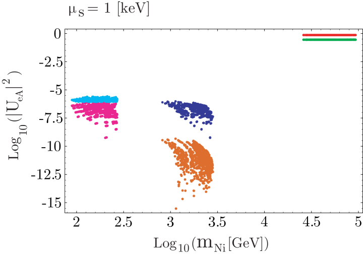
Figure 1: Constraint on the heavy sterile mixing angles in cases of $\mu_{s}=1$ [keV] with varied $\varphi_{1}$, $\varphi_{2}$ and $\sigma$ from $0$ to $2\pi$.

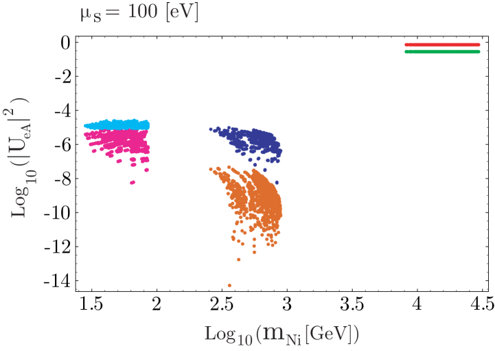
Figure 2: Constraint on the heavy sterile mixing angles in cases of $\mu_{s}=100$ [eV] with varied $\varphi_{1}$, $\varphi_{2}$ and $\sigma$ from $0$ to $2\pi$.

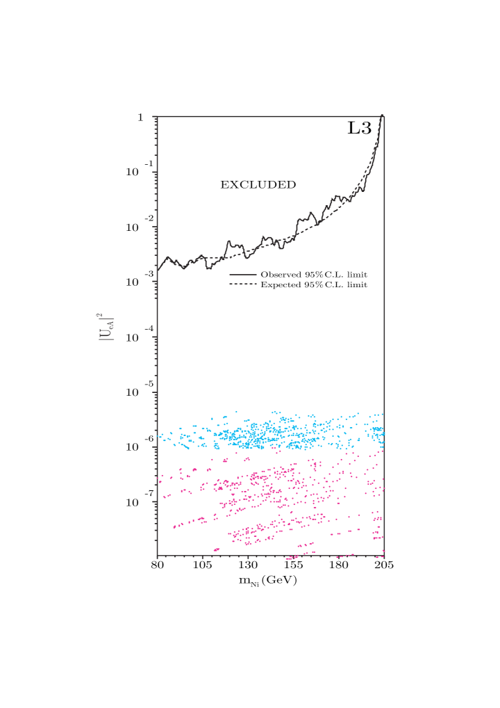
Figure 3: The same figure as Fig. 1 but is overwritten in the LEP experimental bound.

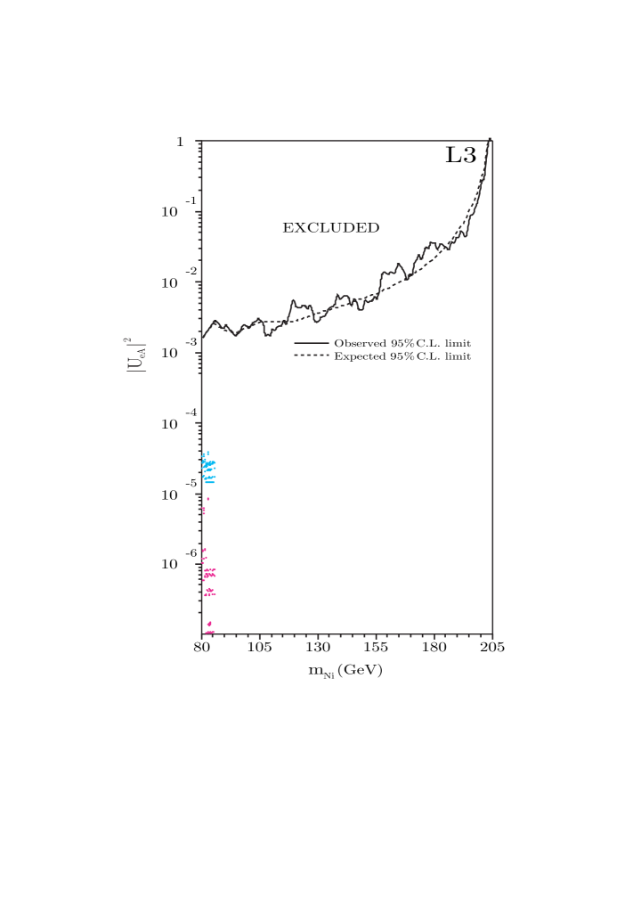
Figure 4: The same figure as Fig. 2 but is overwritten in the LEP experimental bound.

References

- [1] S. Weinberg, Phys. Rev. Lett. 43, 1566 (1979).
- [2] T. Yanagida, in Proceedings of the workshop on the Unified Theory and Baryon Number in the Universe, edited by O. Sawada and A. Sugamoto (KEK, Tsukuba, 1979); M. Gell-Mann, P. Ramond, and R. Slansky, in Supergravity, edited by D. Freedman and P. van Niewenhuizen (north-Holland, Amsterdam 1979); R. N. Mohapatra and G. Senjanović, Phys. Rev. Lett. 44, 912 (1980).
- [3] E. Witten, Nucl. Phys. B 268, 79 (1986).
- [4] R. N. Mohapatra, Phys. Rev. Lett. 56 (1986) 561.
- [5] R. N. Mohapatra and J. W. F. Valle, Phys. Rev. D 34, 1642 (1986).
- [6] T. Fukuyama, A. Ilakovac, T. Kikuchi and K. Matsuda, JHEP 0506, 016 (2005) [arXiv:hep-ph/0503114].
- [7] M. Malinsky, J. C. Romao and J. W. F. Valle, Phys. Rev. Lett. 95, 161801 (2005) [arXiv:hep-ph/0506296].
- [8] E. K. Akhmedov, M. Lindner, E. Schnapka and J. W. F. Valle, Phys. Rev. D 53, 2752 (1996) [arXiv:hep-ph/9509255].
- [9] S. M. Barr, Phys. Rev. Lett. 92, 101601 (2004) [arXiv:hep-ph/0309152].
- [10] S. M. Barr and I. Dorsner, Phys. Lett. B 632, 527 (2006) [arXiv:hep-ph/0507067].
- [11] M. Dittmar, A. Santamaria, M. C. Gonzalez-Garcia and J. W. F. Valle, Nucl. Phys. B 332, 1 (1990).
- [12] P. Achard et al. [L3 Collaboration], Phys. Lett. B 517, 67 (2001) [arXiv:hep-ex/0107014].
- [13] Z. G. Berezhiani, A. Y. Smirnov and J. W. F. Valle, Phys. Lett. B 291, 99 (1992) [arXiv:hep-ph/9207209].
- [14] V. Berezinsky and J. W. F. Valle, Phys. Lett. B 318, 360 (1993) [arXiv:hep-ph/9309214].
- [15] K. S. Babu and R. N. Mohapatra, Phys. Rev. Lett. 70, 2845 (1993) [arXiv:hep-ph/9209215].
- [16] K. Matsuda, Y. Koide and T. Fukuyama, Phys. Rev. D 64, 053015 (2001) [arXiv:hep-ph/0010026].
- [17] K. Matsuda, Y. Koide, T. Fukuyama and H. Nishiura, Phys. Rev. D 65, 033008 (2002) [Erratum-ibid. D 65, 079904 (2002)] [arXiv:hep-ph/0108202];
- [18] T. Fukuyama and N. Okada, JHEP 0211, 011 (2002) [arXiv:hep-ph/0205066].
- [19] B. Bajc, G. Senjanović and F. Vissani, Phys. Rev. Lett. 90, 051802 (2003) [arXiv:hep-ph/0210207].
- [20] H. S. Goh, R. N. Mohapatra and S. P. Ng, Phys. Lett. B 570, 215 (2003) [arXiv:hep-ph/0303055].
- [21] H. S. Goh, R. N. Mohapatra and S. P. Ng, Phys. Rev. D 68, 115008 (2003) [arXiv:hep-ph/0308197].
- [22] B. Dutta, Y. Mimura and R. N. Mohapatra, Phys. Rev. D 69, 115014 (2004) [arXiv:hep-ph/0402113].
- [23] K. Matsuda, Phys. Rev. D 69, 113006 (2004) [arXiv:hep-ph/0401154].
- [24] S. Bertolini and M. Malinsky, Phys. Rev. D 72, 055021 (2005) [arXiv:hep-ph/0504241].
- [25] K. S. Babu and C. Macesanu, Phys. Rev. D 72, 115003 (2005) [arXiv:hep-ph/0505200].
- [26] J. Schechter and J. W. F. Valle, Phys. Rev. D 22, 2227 (1980); M. Doi, T. Kotani, H. Nishiura, K. Okuda and E. Takasugi, Phys. Lett. B 102, 323 (1981).
- [27] H. Fusaoka and Y. Koide, Phys. Rev. D 57, 3986 (1998) [arXiv:hep-ph/9712201].
- [28] H. Murayama, Nucl. Phys. Proc. Suppl. 137, 206 (2004) [arXiv:hep-ph/0410140].
- [29] A. Y. Smirnov, [arXiv:hep-ph/0411194].
- [30] F. Deppisch and J. W. F. Valle, Phys. Rev. D 72, 036001 (2005) [arXiv:hep-ph/0406040].
- [31] A. Ilakovac and A. Pilaftsis, Nucl. Phys. B 437, 491 (1995) [arXiv:hep-ph/9403398].