Chiral symmetry restoration in excited hadrons, quantum fluctuations, and quasiclassics

Abstract

In this paper, we discuss the transition to the semiclassical regime in excited hadrons, and consequently, the restoration of chiral symmetry for these states. We use a generalised Nambu–Jona-Lasinio model with the interaction between quarks in the form of the instantaneous Lorentz–vector confining potential. This model is known to provide spontaneous breaking of chiral symmetry in the vacuum via the standard selfenergy loops for valence quarks. It has been shown recently that the effective single–quark potential is of the Lorentz–scalar nature, for the low–lying hadrons, while, for the high–lying states, it becomes a pure Lorentz vector and hence the model exhibits the restoration of chiral symmetry. We demonstrate explicitly the quantum nature of chiral symmetry breaking, the absence of chiral symmetry breaking in the classical limit as well as the transition to the semiclassical regime for excited states, where the effect of chiral symmetry breaking becomes only a small correction to the classical contributions.

I Introduction

Restoration of $SU(2)_{L}\times SU(2)_{R}$ and $U(1)_{A}$ chiral symmetries of QCD in excited hadrons, both in baryons G1 ; CG and mesons G2 ; G3 ; G5 , was rather unexpected (for a pedagogical overview see Ref. G4 ). Obviously, this phenomenon requires a detailed experimental and theoretical study and can provide a clue to our understanding of confinement, chiral symmetry breaking, and their interrelation. Indeed, it has recently become the subject of a significant theoretical effort OPE ; SWANSON ; DEGRAND ; SHIFMAN ; parity2 .

As it is well known, in the chiral limit, both $SU(2)_{L}\times SU(2)_{R}$ and $U(1)_{A}$ symmetries of the QCD Lagrangian are broken. The spontaneous breaking of $SU(2)_{L}\times SU(2)_{R}\rightarrow SU(2)_{I}$ NJL is directly evidenced through a number of facts, such as i) the absence of any multiplet structure of the $SU(2)_{L}\times SU(2)_{R}$ group in the spectrum of low–lying hadrons, ii) the Goldstone boson nature of the pion, iii) the nonzero value of the quark condensate, which manifestly breaks $SU(2)_{L}\times SU(2)_{R}$ symmetry of the vacuum, and through other observables. The $U(1)_{A}$ symmetry breaking follows from the absence of the multiplets of the $U(1)_{A}$ group low in the spectrum and from a non-Goldstone nature of the $\eta^{\prime}$-meson. The $U(1)_{A}$ symmetry is broken by the axial anomaly of QCD ANOMALY and by the quark condensates in the vacuum CG . There is no one–to–one mapping of the low–lying hadrons of positive and negative parity, thus indicating a strong breaking of both $SU(2)_{L}\times SU(2)_{R}$ and $U(1)_{A}$ symmetries and that chiral symmetry is realised nonlinearly in this part of the hadronic spectrum.

However, already the first radial excitation of the pion, $\pi(1300)$, has an approximately degenerate chiral partner, $f_{0}(1370)$, which is predominantly a $\bar{n}n=\frac{1}{\sqrt{2}}(\bar{u}u+\bar{d}d)$ state CZ . The splitting within the next radially excited doublet, $\pi(1800)$ — $f_{0}(1790)$, is already negligible. There are further radial excitations of the $\pi$ and the $\bar{n}n$ $f_{0}$ states which are approximately degenerate, as well as good chiral multiplets of higher–spin mesons G2 ; G3 . Similarly, already in the $1.7GeV$ mass region, the nucleon well established resonances demonstrate a systematic pattern of an approximate parity doubling. An analogous pattern persists also in the $\Delta$–spectrum, starting from the $1.9GeV$ region, that is, at the same excitation energy with respect to the ground state $\Delta(1232)$ as in the nucleon spectrum. All these experimental facts indicate that the restoration of chiral symmetry happens rather fast. Indeed, the slowest possible rate of the symmetry restoration in mesons is expected to be $\sim 1/n^{3/2}$, where $n$ is the radial quantum number, as was recently shown in Ref. SHIFMAN through the matching of the Operator Product Expansion and the resonance representation of the two–point function.

There are quite unexpected implications of the chiral symmetry restoration. For instance, the chiral partners of the excited vector isovector $\rho$-mesons should be not only the axial–vector isovector $a_{1}$ mesons (see, for example, Ref. OPE ), but also the axial–vector isoscalar $h_{1}$ mesons G3 . Consequently, there must be excited $\rho$–mesons of two kinds, those which form $(1,0)\oplus(0,1)$ multiplets, together with the $a_{1}$–mesons, and those which fill in $(1/2,1/2)$ chiral multiplets, together with the $h_{1}$–mesons G3 ; SHIFMAN . Actually, similar rules are valid also for all possible mesons with $J\geqslant 1$ G3 . Consequently, all highly excited hadrons can be viewed as colour–electric strings with chiral quarks at the ends G5 .

While the role of different gluonic interactions of QCD, which could be responsible for chiral symmetry breaking, is not yet clear — these could be instantons, nonperturbative resummation of perturbative gluon exchanges, gluodynamics responsible for the QCD string formation, or something else, — the most fundamental reason of the chiral symmetry restoration in excited hadrons is universal G6 . Namely, both $SU(2)_{L}\times SU(2)_{R}$ and $U(1)_{A}$ symmetries breaking results from quantum fluctuations of the quark fields (that is, loops). However, for highly excited states a quasiclassical regime necessarily takes place. Semiclassically, the contribution of quantum fluctuations is suppressed, relative to the classical contributions, by the factor of $\hbar/{\cal S}$, where ${\cal S}$ is the classical action of the intrinsic motion in the system (that is, the full action of the hadron, in terms of quark and gluon degrees of freedom, minus the action of the centre–of–mass motion). Since, for highly excited hadrons, ${\cal S}\gg\hbar$, then the symmetries of the classical Lagrangian must be restored.

While this argument is quite general and solid, it does not provide us with any detailed microscopic picture of the symmetry restoration. Then, in the absence of controllable analytic solutions of QCD, such an insight can be obtained only through models. It is the purpose of this paper to get such an insight.

Before discussing the details of the particular model to be invoked, it is instructive to outline the minimal set of requirements for such a model. It must be i) relativistic, ii) chirally symmetric, and iii) able to provide a mechanism of spontaneous breaking of chiral symmetry, iv) it should contain confinement, in order to be able to address the issue of excited states, and v) it must explain the restoration of chiral symmetry for excited states. It is highly nontrivial indeed to meet all these requirements with one and the same model. For example, the famous Nambu and Jona-Lasinio model (NJL) NJL ; REVIEWS or its specific realisations, like the instanton–liquid model SHURYAK , cannot be applied to excited hadrons as a matter of principle, since they do not contain confinement as an intrinsic feature, even though these models suggest an insight into chiral symmetry breaking in the vacuum and into physics of the lowest–lying hadrons. On the contrary, naive quark models, with confinement postulated in the form of a raising potential between the constituent quarks, do not contain any mechanism of chiral symmetry breaking and hence must fail not only for the low–lying hadronic states, but also for highly excited ones G4 ; G5 .

There is a model, however, which does incorporate all required elements. This is the generalised Nambu–Jona-Lasinio (GNJL) model with the instantaneous vector confining kernel Orsay ; Orsay2 ; Lisbon . This model is similar in spirit to the large–$N_{C}$ ’t Hooft model in 1+1 dimensions tHooft — in the latter confinement being provided by the linearly rising Coulomb potential. An advantage of the GNJL model is that it can be applied in 3+1 dimensions to systems of an arbitrary spin. In this model, confinement of quarks is guaranteed due to the instantaneous infinitely raising (for example, linear) potential, which can be also supplied by extra ingredients, like the colour Coulomb potential, for example. Then chiral symmetry breaking can be described by the standard summation of the valence quark selfinteraction loops (the mass–gap equation), while mesons are obtained from the Bethe–Salpeter equation for the quark–antiquark bound states. It was demonstrated in Ref. parity2 that, for the low–lying states, where chiral symmetry breaking is important, this model leads to an effective Lorentz–scalar binding interquark potential, while for the high–lying states, such an effective potential becomes a pure Lorentz spatial vector. As a result, the model does provide chiral symmetry restoration. Besides, this model has an obvious advantage as it is tractable and thus can be used as a laboratory to get a microscopical insight into the restoration of chiral symmetry for excited hadrons. It is the purpose of this paper to demonstrate, in the framework of the GNJL model, the transition to the quasiclassical regime for excited mesons and clarify the role of quantum fluctuations in these systems.

II Generalised Nambu–Jona-Lasinio model

II.1 Introduction to the model and general remarks

In this chapter, we give a short introduction to the GNJL chiral quark model, called after the original paper NJL , and which is known to be a reliable testground for various low–energy phenomena in QCD Orsay ; Orsay2 ; Lisbon . The model is described by the Hamiltonian

$$\hat{H}=\int d^{3}x\bar{\psi}(\vec{x},t)\left(-i\vec{\gamma}\cdot\vec{\bigtriangledown}+m\right)\psi(\vec{x},t)+\frac{1}{2}\int d^{3}xd^{3}y\;J^{a}_{\mu}(\vec{x},t)K^{ab}_{\mu\nu}(\vec{x}-\vec{y})J^{b}_{\nu}(\vec{y},t),$$ (1)

with the quark current–current ($J_{\mu}^{a}(\vec{x},t)=\bar{\psi}(\vec{x},t)\gamma_{\mu}\frac{\lambda^{a}}{2}\psi(\vec{x},t)$) interaction parametrised by the instantaneous confining kernel $K^{ab}_{\mu\nu}(\vec{x}-\vec{y})$ of a generic form.

The model (1), with the full kernel $K^{ab}_{\mu\nu}$ restricted to the $K^{ab}_{00}$ component only, was suggested in the mid-eighties Orsay ; Orsay2 and an instability of the chirally–symmetric vacuum was demonstrated for the variety of confining potentials of the form $|{\vec{x}}|^{\alpha}$. Later, in the series of papers Lisbon , the given theory was rederived in a generalised form through the introduction of Cooperlike ${}^{3}P_{0}$ quark-antiquark pairs, with the spatial components of the kernel, $K^{ab}_{ij}$, included, which led to modifications of the mass–gap equation. Constraints on the relative strengths of the confining potentials of various Lorentz structure were imposed, in order to maintain a divergence–free mass–gap equation. In addition, the quark models of this class are demonstrated to fulfill the well-known low–energy theorems, such as the Gell-Mann–Oakes–Renner relation GOR (for an early derivation see, for example, Ref. Orsay2 ), Goldberger–Treiman relation GT , Adler selfconsistency zero ASC , the Weinberg theorem Wein (derived for the model (1) in Ref. EmilCota ), and so on. A convenient analytic formalism to derive such low–energy theorems was suggested in Ref. BicudAp , which is based on the approach of Salpeter equations, put forward in the set of papers Lisbon . The axial anomaly and the $\pi\gamma\gamma$ coupling constant can be derived naturally in the framework of the given model as well, following, for example, the lines of the textbook CL and using the asymptotic freedom and the Ward identity for the dressed axial vertex BicudAp (see also Ref. pi2g for an independent derivation of this relation in the Dyson–Schwinger approach to the dressed quark propagator). Finally, the structure of the Hamiltonian (1) can be traced back to QCD in the Coulomb gauge coulg .

In this paper, we use the simplest form of the kernel compatible with the requirement of confinement Lisbon ,

$$K^{ab}_{\mu\nu}(\vec{x}-\vec{y})=g_{\mu 0}g_{\nu 0}\delta^{ab}V_{0}(|\vec{x}-\vec{y}|),$$ (2)

with the powerlike confining potential,

$$V_{0}(|\vec{x}|)=K_{0}^{\alpha+1}|\vec{x}|^{\alpha},\quad 0\leqslant\alpha\leqslant 2.$$ (3)

Moreover, in order to make contact with the phenomenology of quarkonia, we stick to the linearly growing potential (see, for example, Ref. linear ), which corresponds to the case $\alpha=1$ of the general form (3). In the chiral limit, $m=0$, the only remaining dimensional parameter is the strength of the potential $K_{0}$ (in case of the linear confinement, we use the conventional notation of the string tension $K_{0}^{2}=\sigma_{0}$). It is remarkable, as mentioned in the introduction, that, in two dimensions, the well–known ’t Hooft model for QCD₂ tHooft in the large–$N_{C}$ limit and considered in the axial gauge BG ; 2d , also belongs to the theories of the class (1). In this case, the approximations of the instantaneous nature of the interquark interaction and the absence of higher–order kernels $K_{\mu\nu\lambda}^{abc},\ldots$ are exact and do not require any justification. In four dimensions, such approximations are supported by independent studies of the properties of the QCD vacuum. Indeed, the relative smallness of the gluonic correlation length, measured on the lattice Tg , argues in favour of validity of the instantaneous quark kernel, whereas the Casimir scaling, suggested long ago cs1 and recently confirmed by lattice calculations cs2 , supports the neglect of higher–order kernels parametrising triple, quartic, and so on quark–current vertices in the Hamiltonian (1). Recently, the model (1) was considered from the point of view of the chiral symmetry restoration high in the spectrum of mesons and, indeed, the parity doubling was demonstrated to occur above the scale of about $2.5GeV$, regardless of the explicit form of the confining potential (3) parity2 . Although, in real QCD, the chiral symmetry restoration in the hadronic spectrum seems to occur somewhat faster — possibly due to other nonconfining contributions to the interquark interaction — the found estimate for the restoration scale is reasonable.

One can conclude, therefore, that the model under consideration, as a beautiful testground for real QCD, provides a reliable source of information about various phenomena related to chiral symmetry, ranging from its spontaneous breaking in the lower part of hadronic spectrum and up to its effective restoration high in the spectrum. In this paper, we employ the model (1) in order to illustrate some general aspects of the phenomenon of spontaneous breaking of chiral symmetry — namely, to argue its intrinsically quantum nature and to exemplify its restoration in the hadronic spectrum as a general effect of restoration of the classical symmetries of the fundamental QCD Lagrangian.

II.2 Chiral symmetry breaking

Figure 1: Graphical representation of the equations for the dressed quark propagator, Eq. (5), and for the quark mass operator, Eq. (7).

The key idea of the BCS BCS approach to spontaneous breaking of chiral symmetry in the class of Hamiltonians described by Eq. (1) is the Dyson series for the quark propagator, which takes the form, schematically:

$$S=S_{0}+S_{0}\Sigma S_{0}+S_{0}\Sigma S_{0}\Sigma S_{0}+\ldots,$$ (4)

with $S_{0}$ and $S$ being the bare– and the dressed–quark propagators, respectively, $\Sigma$ is the quark mass operator (see Fig. 1). The series (4) can be summed up to produce the Dyson–Schwinger equation,

$$S=S_{0}+S_{0}\Sigma S,$$ (5)

with the formal solution being

$$S^{-1}(p_{0},{\vec{p}})=S_{0}^{-1}(p_{0},{\vec{p}})-\Sigma({\vec{p}}),$$ (6)

where the mass operator independence of the energy $p_{0}$ follows from the instantaneous nature of the interaction — see also Eqs. (7) and (14) below. The expression for the mass operator through the dressed–quark propagator (see Fig. 1) reads:

$$i\Sigma(\vec{p})=C_{F}\int\frac{d^{4}k}{(2\pi)^{4}}V_{0}(\vec{p}-\vec{k})\gamma_{0}S(\vec{k},k_{0})\gamma_{0},\quad C_{F}=\frac{N_{C}^{2}-1}{2N_{C}},$$ (7)

with both quark–quark–potential vertices being bare momentum–independent vertices $\gamma_{0}$. This corresponds to the so-called rainbow approximation which is well justified in the limit of the large number of colours $N_{C}$. We assume this limit in what follows. Then all nonplanar (such as nonrainbow and those dressing the vertex $\gamma_{0}$) diagrams appear suppressed by $N_{C}$ and can be consecutively removed from the theory (see Fig. 2(a) for the examples of the planar and Fig. 2(b) for nonplanar diagrams). Eqs. (5) and (7) together produce a closed set of equations, equivalent to a single nonlinear equation for the mass operator,

$$i\Sigma(\vec{p})=\int\frac{d^{4}k}{(2\pi)^{4}}V(\vec{p}-\vec{k})\gamma_{0}\frac{1}{S_{0}^{-1}(k_{0},{\vec{k}})-\Sigma({\vec{k}})}\gamma_{0},$$ (8)

where the fundamental Casimir operator $C_{F}$ is absorbed to the potential, $V({\vec{p}})=C_{F}V_{0}({\vec{p}})$, by introducing the fundamental string tension $\sigma=C_{F}\sigma_{0}$.

Figure 2: Planar (figure (a)) and nonplanar, suppressed by $N_{C}$, (figure (b)) diagrams.

As it often happens in the theories with strong interaction, Eq. (8) may have multiple solutions. One of this solutions is given by the perturbative series, schematically,

$$\Sigma=\int d^{4}k\;V\gamma_{0}S_{0}\gamma_{0}+\int d^{4}k\;d^{4}q\;V^{2}\gamma_{0}S_{0}\gamma_{0}S_{0}\gamma_{0}S_{0}\gamma_{0}+\ldots,$$ (9)

which converges fast in the weak interaction limit. Below we discuss in detail another, nonperturbative, solution to Eq. (8). In the meantime, alternatively, the series (9) can be viewed as an expansion in powers of the Planck constant $\hbar$. Indeed, the mass operator is defined as the quark selfinteraction loop integral which, being a purely quantum effect, is to be proportional to $\hbar$. To see this explicitly, let us restore $\hbar$’s in the expression for the mass operator (8). To this end, defining the confining potential through the area law for the average of the closed Wilson loop (for completeness, we restore here the speed of light $c$ as well),

$$\langle W(C)\rangle=\exp\left[-\frac{\sigma A}{\hbar c}\right],$$ (10)

with $\sigma$ and $A$ being the string tension and the area of the minimal Euclidean surface bounded by the contour $C$, respectively, we extract the potential, for the rectangular loop $C$:

$$\frac{\sigma A}{\hbar c}=\frac{\sigma R\times(cT)}{\hbar c}=\frac{1}{\hbar}\int_{0}^{T}dt\sigma R=\frac{1}{\hbar}\int_{0}^{T}dt\times{\rm potential}.$$ (11)

In the last formula, we restored both $\hbar$ and $c$, for the sake of transparency. However, in most formulae below, in order to simplify notations, we do now show the speed of light $c$, restoring it only when necessary. Therefore, from Eq. (11), we find the potential to be $V(r)=\sigma r$, which does not contain $\hbar$ and is expected to remain finite in the formal classical limit of $\hbar\to 0$. This constitutes the conjecture of classical confinement, which we use throughout the paper. Now, the Fourier transform of this potential is

$$V({\vec{p}})=\int d^{3}xe^{i\frac{{\vec{p}}{\vec{x}}}{\hbar}}\sigma|{\vec{x}}|=-\frac{8\pi\sigma\hbar^{4}}{p^{4}}=\hbar^{4}\tilde{V}({\vec{p}}),$$ (12)

where $\tilde{V}({\vec{p}})$ does not contain $\hbar$. Then, in Eq. (8), the factor $\hbar^{4}$, from the Fourier transform of the potential (12), will cancel $\hbar$’s in the denominator, coming from $\frac{d^{4}k}{(2\pi\hbar)^{4}}$, the only remaining Planck constant being the one multiplying the entire integral in Eq. (8), which is easily restored for dimensional reasons. Thus, we find:

$$i\Sigma(\vec{p})=\hbar\int\frac{d^{4}k}{(2\pi)^{4}}\tilde{V}(\vec{p}-\vec{k})\gamma_{0}\frac{1}{S_{0}^{-1}(k_{0},{\vec{k}})-\Sigma({\vec{k}})}\gamma_{0}.$$ (13)

In other words, as easily seen from Eq. (13), each power of the potential brings an extra loop integral and, as a result, an extra power of $\hbar$.

To proceed, we use a convenient parametrisation of the mass operator $\Sigma({\vec{p}})$, in the form Lisbon :

$$\Sigma(\vec{p})=[A_{p}-m]+(\vec{\gamma}\hat{\vec{p}})[B_{p}-p],$$ (14)

so that the dressed–quark Green’s function (6) becomes

$$S^{-1}(\vec{p},p_{0})=\gamma_{0}p_{0}-(\vec{\gamma}\hat{\vec{p}})B_{p}-A_{p},$$ (15)

where, due to the instantaneous nature of the interquark interaction, the time component of the four–vector $p_{\mu}$ is not dressed.

It is easily seen from Eq. (15) that the functions $A_{p}$ and $B_{p}$ represent the scalar part and the space–vectorial part of the effective Dirac operator. In the chiral limit, $A_{p}$ vanishes, unless chiral symmetry is broken spontaneously. It is convenient, therefore, to introduce an angle, known as the chiral angle $\varphi_{p}$, according to the definition:

$$\tan\varphi_{p}=\frac{A_{p}}{B_{p}},$$ (16)

and varying in the range $-\frac{\pi}{2}<\varphi_{p}\leqslant\frac{\pi}{2}$, with the boundary conditions $\varphi(0)=\frac{\pi}{2}$, $\varphi(p\to\infty)\to 0$.

The selfconsistency condition for the parametrisation (14) of the nonlinear Eq. (13) requires that the chiral angle obeys a nonlinear equation — the mass–gap equation,

$$A_{p}\cos\varphi_{p}-B_{p}\sin\varphi_{p}=0,$$ (17)

where

$$A_{p}=m+\frac{\hbar}{2}\int\frac{d^{3}k}{(2\pi)^{3}}\tilde{V}(\vec{p}-\vec{k})\sin\varphi_{k},\quad B_{p}=p+\frac{\hbar}{2}\int\frac{d^{3}k}{(2\pi)^{3}}\;(\hat{\vec{p}}\hat{\vec{k}})\tilde{V}(\vec{p}-\vec{k})\cos\varphi_{k}.$$ (18)

Notice that both functions $A_{p}$ and $B_{p}$ contain classical and quantum contributions, the latter coming from loops. For free particles, only the classical part survives and the chiral angle (16) reduces to the free Foldy angle, $\varphi_{p}^{(0)}=\arctan\frac{m}{p}$, which diagonalises the free Dirac Hamiltonian $H=\vec{\alpha}{\vec{p}}+\beta m$. The deep connection between the chiral and the Foldy angles holds also for nontrivial dynamically generated solutions to the mass–gap Eq. (17) (see, for example, 2d ; NR1 ).

The dispersive law of the dressed quark can be built then as

$$E_{p}=A_{p}\sin\varphi_{p}+B_{p}\cos\varphi_{p},$$ (19)

and it differs drastically from the free–quark energy, even becoming negative in the low–momentum region. The latter behaviour is important in order to explain a very small pion mass Orsay ; Lisbon ; NR1 .

It was demonstrated in the pioneering papers Orsay that, for confining potentials, the mass–gap equation (17) always possesses nontrivial solutions which break chiral symmetry by generating a nontrivial masslike function $A_{p}$, even for vanishing quark current mass. These solutions are given by smooth decreasing functions which start at $\frac{\pi}{2}$ at the origin, with the slope inversely proportional to the scale of chiral symmetry breaking, generated by these solutions. At large momenta they approach zero fast (see Fig. 3).

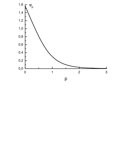
Figure 3: Nontrivial solution to the mass–gap Eq. (17) with $m=0$ and for the linear confinement (see, for example, Refs. replica1 ; replica4 for the details). The momentum $p$ is given in the units of $\sqrt{\sigma}$.

If the density of the vacuum energy is calculated for these nontrivial solutions as

$$E_{\rm vac}[\varphi_{p}]=-\frac{g}{2}\int\frac{d^{3}p}{(2\pi\hbar)^{3}}\left([A_{p}+m]\sin\varphi_{p}+[B_{p}+p]\cos\varphi_{p}\right),\quad g=(2s+1)N_{C}N_{f},$$ (20)

where the degeneracy factor $g$ counts the number of independent quark degrees of freedom ($s=\frac{1}{2}$ is the quark spin, $N_{C}$ and $N_{f}$ are the number of colours and the number of flavours, respectively), and is compared to the trivial, unbroken, vacuum energy density, then one can see that, possessing a lower energy,

$$\Delta E_{\rm vac}=E_{\rm vac}[\varphi_{p}]-E_{\rm vac}[\varphi_{p}^{(0)}]<0,$$ (21)

the broken phase is energetically favourable and the unbroken phase is, therefore, unstable Orsay . The new, broken, vacuum is known as the BCS vacuum of the theory. A detailed qualitative and numerical investigation of chiral symmetry breaking for various powerlike confining potentials was performed in Ref. replica4 .

II.3 Breakdown of the expansion for $\varphi_{p}$ in powers of $\hbar$

It was demonstrated, in the previous chapter, that all nontrivial solutions to the mass–gap Eq. (17) appear entirely due to loops and they are, therefore, of an intrinsically quantum nature. In this chapter, we consider the mass–gap equation more closely and study the expansion of the chiral angle in powers of $\hbar$.

For the sake of transparency, we write the mass–gap equation in the explicit form and restore both the Planck constant $\hbar$ and the speed of light $c$ in it,

$$pc\sin\varphi_{p}-mc^{2}\cos\varphi_{p}=\frac{\hbar}{2}\int\frac{d^{3}k}{(2\pi)^{3}}\tilde{V}({\vec{p}}-{\vec{k}})\left[\cos\varphi_{k}\sin\varphi_{p}-(\hat{\vec{p}}\hat{\vec{k}})\sin\varphi_{k}\cos\varphi_{p}\right].$$ (22)

Consider the chiral limit of $m=0$ first. Then, in the formal classical limit of $\hbar\to 0$, the selfenergy (13) as well as the right–hand side of Eq. (22) vanishes, and the only solution of this equation is trivial, $\varphi_{p}=0$. In view of the discussion of the previous chapter, this result is obvious since, being a genuine quantum entity — parametrising loop integrals — $\varphi_{p}$ should vanish in the classical limit. A naive attempt to search for solutions of Eq. (22) in the form of the formal expansion in $\hbar$, $\varphi_{p}=\hbar\times f_{1}(p)+\hbar^{2}\times f_{2}(p)+\ldots$, fails — all coefficients vanish. The reason of such a failure can be considered from two viewpoints. Formally, to perform such an expansion, one is to build a quantity, $\cal S$, with the dimension of the classical action, in order to perform the actual expansion, $\varphi_{p}=\frac{\hbar}{\cal S}\times f_{1}(p)+\frac{\hbar^{2}}{{\cal S}^{2}}\times f_{2}(p)+\ldots$. With only two dimensional parameters in hand, the string tension $\sigma$ and the speed of light $c$, it is not possible to build such an action. On the other hand, one can arrive at the same conclusion by a direct inspection of Eq. (22). Indeed, the chiral angle is a dimensionless function of the form $\varphi_{p}=f_{0}(p/(\mu c))$, where the mass scale $\mu$ is to be built out of the dimensional parameters of the theory. In order to build this scale, let us introduce dimensionless variables in the integral, ${\vec{p}}=\mu c{\vec{x}}$ and ${\vec{k}}=\mu c{\vec{y}}$, and define $\mu$ such that the resulting equation defines only the profile of the chiral angle and does not contain any scale at all. The result is $\mu=\sqrt{\sigma\hbar c}/c^{2}$ and we end up with a nonanalytic dependence of $\varphi_{p}$ on the Planck constant. This is easily seen, for example, from the low–momentum expansion of $\varphi_{p}$,

$$\varphi_{p}\mathop{\approx}\limits_{p\to 0}\frac{\pi}{2}-{\rm const}\frac{pc}{\mu c^{2}}+\ldots=\frac{\pi}{2}-{\rm const}\frac{pc}{\sqrt{\sigma\hbar c}}+\ldots.$$

As $\hbar$ vanishes, the chiral angle gets steeper and steeper at the origin, approaching the trivial solution $\varphi_{p}=0$ for all $p$’s and, in the limit of $\hbar\rightarrow 0$, we cease to have a low–momentum expansion of $\varphi_{p}$. Such a collapse of the chiral angle in the classical limit has a rather deep physical reason. Indeed, the pseudounitary operator creating the broken BCS vacuum $|0\rangle$ from the unbroken vacuum $|0\rangle_{0}$ is Lisbon ; replica2

$$|0\rangle=U_{0}|0\rangle_{0},\quad U_{0}=e^{Q^{\dagger}-Q},\quad Q^{\dagger}=\frac{1}{2}\int\frac{d^{3}p}{(2\pi\hbar)^{3}}\varphi_{p}C_{p}^{\dagger},$$ (23)

$$C_{p}^{\dagger}=[b^{\dagger}_{\uparrow}(\vec{p}),b^{\dagger}_{\downarrow}(\vec{p})]\mathfrak{M}_{{}^{3}P_{0}}\left[\begin{array}[]{c}d^{\dagger}_{\uparrow}(\vec{p})\\ d^{\dagger}_{\downarrow}(\vec{p})\end{array}\right],\quad\mathfrak{M}_{{}^{3}P_{0}}=(\vec{\sigma}\hat{\vec{p}})i\sigma_{2},$$ (24)

where $\sigma$’s are the $2\times 2$ Pauli matrices. Therefore, the chiral angle is nothing but the wave function of the BCS ${}^{3}P_{0}$ quark–antiquark pairs in the vacuum, created with the operator $C_{p}^{\dagger}$. Besides that, the chiral angle (in the form of $\sin\varphi_{p}$) defines the wave function of the chiral pion Orsay ; Lisbon ; NR1 . In the classical limit, wave functions of quantum systems are known to collapse and no expansion in powers of $\hbar$ is possible. We arrive, therefore, at the purely “nonperturbative” in $\hbar$ solution to the mass–gap equation and thus an inevitable breakdown of the expansion of the chiral angle $\varphi_{p}$ in $\hbar$. It is instructive to go now slightly beyond the chiral limit and to switch on a small current quark mass $m$. Working on top of the chirally nonsymmetric BCS vacuum, one can incorporate a small $m$ as a perturbation, in the spirit of the standard chiral perturbation theory, building an infinite series of corrections to the leading regime $\varphi_{p}=f_{0}(pc/\sqrt{\sigma\hbar c})$, suppressed by the small parameter $\frac{mc^{2}}{\sqrt{\sigma\hbar c}}$,

$$\varphi_{p}=\sum_{n=0}^{\infty}\left(\frac{mc^{2}}{\sqrt{\sigma\hbar c}}\right)^{n}f_{n}\left(\frac{pc}{\sqrt{\sigma\hbar c}}\right),$$ (25)

where the leading term — the function $f_{0}$ — is known only numerically and is depicted in Fig. 3.

However, beyond the chiral limit, the nonanalytic in $\hbar$ behaviour of the chiral angle is “smeared” by the quark mass, so that $\varphi_{p}$ does support now an expansion in $\hbar$ — this can be verified by a direct investigation of the mass–gap Eq. (22). One can also arrive at the same conclusion using general qualitative arguments. Indeed, for a nonvanishing quark mass $m$, it is possible to build the quantity with the dimension of the classical action, ${\cal S}\sim\frac{m^{2}c^{3}}{\sigma}$, so that the actual parameter of the expansion appears to be $\frac{\sigma\hbar c}{(mc^{2})^{2}}$ and the mass–gap Eq. (22) admits a solution in the form of a “perturbative” series in powers of $\hbar$,

$$\varphi_{p}=\sum_{n=0}^{\infty}\left(\frac{\sigma\hbar c}{(mc^{2})^{2}}\right)^{n}\tilde{f}_{n}\left(\frac{p}{mc}\right),$$ (26)

the leading term giving just the free solution, $\tilde{f}_{0}=\arctan\frac{mc}{p}$. As a matter of fact, this “perturbative” solution is represented by the series for the quark selfenergy (9).

It is easy to notice that the two expansions given by Eqs. (25) and (26) follow from one and the same solution to the mass–gap equation. However, while the expansion (25) is appropriate around the chiral limit $m=0$ and beyond the classical limit, $\hbar\neq 0$ (the expansion (26) fails in this region), for $m\gg\frac{\sqrt{\sigma\hbar c}}{c^{2}}$, the expansion (26) is much better than that of Eq. (25). Notice that there is no one–to–one correspondence between the sets of functions $\{f_{n}\}$ and $\{\tilde{f}_{n}\}$ (for example, the function $f_{0}$, depicted in Fig. 3, approaches zero as $1/p^{5}$ at large $p$’s, whereas the asymptotic behaviour of $\tilde{f}_{0}$ is much slower, only $1/p$).

In conclusion, notice that Eqs. (25) and (26) explicitly define two different regimes, according to the value of the parameter $\frac{m}{\sqrt{\sigma}}$. Chiral symmetry and its spontaneous breaking are relevant for $m\ll\sqrt{\sigma}$ — the regime (25), while the “heavy–quark physics” is adequate in the opposite limit of $m\gg\sqrt{\sigma}$ — the regime (26).

III Parity doubling for highly excited hadrons

Figure 4: Graphical representation of the Bethe–Salpeter Eq. (27) for the quark–antiquark bound state, in the ladder approximation.

In this chapter, we consider the spectrum of heavy–light mesons and demonstrate explicitly the quantum nature of the splitting within chiral doublets. To this end, we derive the bound–state equation for the quarkonium made of a static antiquark, placed at the origin, and a light quark. We follow the lines of Ref. parity2 .

The Bethe–Salpeter equation for the mesonic Salpeter amplitude $\chi({\vec{p}};M)$, depicted graphically in Fig. 4, reads:

$$\chi({\vec{p}};M)=-i\int\frac{d^{4}k}{(2\pi)^{4}}V(\vec{p}-\vec{k})\;\gamma_{0}S_{q}({\vec{k}},k_{0}+M/2)\chi({\vec{k}};M)S_{\bar{Q}}({\vec{k}},k_{0}-M/2)\gamma_{0},$$ (27)

where the light–quark propagator (6) (we use the subscript $q$ in order to distinguish it from the static–particle propagator, labelled by $\bar{Q}$) can be written as a sum of the positive– and negative–energy parts Lisbon ; kw ,

$$S_{q}({\vec{p}},p_{0})=\frac{\Lambda^{+}({\vec{p}})\gamma_{0}}{p_{0}-E_{p}+i\epsilon}+\frac{{\Lambda^{-}}({\vec{p}})\gamma_{0}}{p_{0}+E_{p}-i\epsilon},$$ (28)

with the dressed projectors being

$$\Lambda^{\pm}(\vec{p})=T_{p}P_{\pm}T_{p}^{\dagger},\quad P_{\pm}=\frac{1\pm\gamma_{0}}{2},\quad T_{p}=\exp{\left[-\frac{1}{2}(\vec{\gamma}\hat{\vec{p}})\left(\frac{\pi}{2}-\varphi_{p}\right)\right]}.$$ (29)

Eq. (27) is written in the ladder approximation which, similarly to the rainbow approximation for the quark mass operator, is well controlled in the large–$N_{C}$ limit.

Similarly, for the static particle, the chiral angle is simply $\varphi_{\bar{Q}}(p)=\frac{\pi}{2}$, so that its Green’s function takes a very simple form,

$$S_{\bar{Q}}({\vec{p}},p_{0})=\frac{P_{+}\gamma_{0}}{p_{0}-m_{\bar{Q}}+i\epsilon}+\frac{P_{-}\gamma_{0}}{p_{0}+m_{\bar{Q}}-i\epsilon}.$$ (30)

Now, defining the vertex $\varGamma(\vec{p})$, rotated with the light–quark Foldy operator $T^{\dagger}_{p}$ kw from the left and with the heavy–quark Foldy operator, reduced to unity, from the right,

$$\varGamma(\vec{p})=T_{p}^{\dagger}\left[\int\frac{dp_{0}}{2\pi}S_{q}(\vec{p},p_{0}+M/2)\chi(\vec{p};M)S_{\bar{Q}}(\vec{p},p_{0}-M/2)\right]\hat{1},$$ (31)

and performing the energy integration in Eq. (27), we arrive at the matrix equation for the new vertex,

$$(E-E_{p})\varGamma(\vec{p})=P_{+}\left[\int\frac{d^{3}k}{(2\pi)^{3}}V(\vec{p}-\vec{k})T_{p}^{\dagger}T_{k}\varGamma(\vec{k})\right]P_{-}.$$ (32)

For the sake of convenience, we defined the energy excess over the static–particle mass, $E=M-m_{\bar{Q}}$. Due to the projectors on the right–hand side of Eq. (32), the matrix $\varGamma(\vec{p})$ should be searched in the form

$$\varGamma(\vec{p})=\left(\begin{array}[]{cc}0&\psi(\vec{p})\\ 0&0\end{array}\right)={\psi(\vec{p})\choose 0}_{q}\otimes(0\;1)_{\bar{Q}},$$ (33)

which is valid for $M>0$. For negative $M$’s, when the quark and the antiquark are interchanged, the matrix $\varGamma(\vec{p})$ obeys an equation similar to Eq. (32) and takes the form:

$$\varGamma(\vec{p})=\left(\begin{array}[]{cc}0&0\\ \psi(\vec{p})&0\end{array}\right)={0\choose\psi(\vec{p})}_{\bar{q}}\otimes(1\;0)_{Q}.$$ (34)

Thus, in view of a very passive role played by the static constituent, the heavy–light meson wave function $\Psi(\vec{p})$ can be identified with the light–particle wave function 2d ; parity2 ,

$$\Psi(\vec{p})_{|M>0}={\psi(\vec{p})\choose 0},\quad\Psi(\vec{p})_{|M<0}={0\choose\psi(\vec{p})},$$

where $\psi({\vec{p}})$ obeys a Schrödingerlike equation parity2 ,

$$E_{p}\psi(\vec{p})+\int\frac{d^{3}k}{(2\pi)^{3}}V({\vec{p}}-{\vec{k}})\left[C_{p}C_{k}+({\vec{\sigma}}\hat{{\vec{p}}})({\vec{\sigma}}\hat{{\vec{k}}})S_{p}S_{k}\right]\psi(\vec{k})=E\psi(\vec{p}),$$ (35)

with $C_{p}=\cos\frac{1}{2}\left(\frac{\pi}{2}-\varphi_{p}\right)$ and $S_{p}=\sin\frac{1}{2}\left(\frac{\pi}{2}-\varphi_{p}\right)$.

The bound–state Eq. (35) was studied in detail in Ref. parity2 and it was demonstrated to support parity doublers high in the spectrum of heavy–light bound states. Moreover, a relation between chiral symmetry restoration for highly excited states and the Lorentz nature of the effective interquark interaction was established in the same work. Following the lines of the cited paper and performing the reversed Foldy–Wouthuysen transformation, with the help of the operator $T_{p}$, one can derive a Diraclike effective one–particle equation for the light–quark Foldy–counter–rotated wave function, $\tilde{\Psi}(\vec{p})=T_{p}\Psi(\vec{p})$, in coordinate space,

$$(c{\vec{\alpha}}{\vec{p}}+\beta mc^{2})\tilde{\Psi}({\vec{x}})+\frac{\sigma}{2}\int d^{3}z\left(\vphantom{A^{2}}|{\vec{x}}|+|{\vec{z}}|-|{\vec{x}}-{\vec{z}}|\right)U({\vec{x}}-{\vec{z}})\tilde{\Psi}({\vec{z}})=E\tilde{\Psi}({\vec{x}}),$$ (36)

with the unitary matrix

$$U({\vec{x}})=\int\frac{d^{3}p}{(2\pi\hbar)^{3}}U({\vec{p}})e^{-i\frac{{\vec{p}}{\vec{x}}}{\hbar}},\quad U({\vec{p}})=\beta\sin\varphi_{p}+({\vec{\alpha}}\hat{{\vec{p}}})\cos\varphi_{p}.$$ (37)

We have restored, in Eqs. (36) and (37), the speed of light and the Planck constant. The Lorentz nature of the effective interquark interaction in the Diraclike Eq. (36) is governed by the structure of the matrix $U$, that is, by the value of the chiral angle $\varphi_{p}$. Indeed, for $\varphi_{p}\approx\frac{\pi}{2}$, the effective interaction is scalar, so that no parity doublers can appear. On the contrary, for a vanishing chiral angle, the interaction becomes vectorial, Eq. (36) respects chiral symmetry and, as a result, this symmetry manifests itself in the spectrum, in the form of degeneracy in mass between the states with opposite parity. This obviously happens to highly excited mesons, since the mean relative interquark momentum in such states is large, and, consequently, the corresponding value of the chiral angle is small (see Fig. 3). Notice, however, that as discussed above, in the chiral limit, a nontrivial angle $\varphi_{p}$ appears entirely due to quantum fluctuations (loops) and it is a function of the argument $pc/\sqrt{\sigma\hbar c}$. Then, considering large relative momenta is equivalent to taking the formal classical limit of $\hbar\to 0$. In this limit, it follows from the mass–gap equation that $\sin\varphi_{p}=0$, consequently Eq. (36) becomes completely classical with the Lorentz–vector spatial potential. We see, therefore, that, in agreement with general expectations G6 , the effects of quantum fluctuations fade out in the semiclassical region of highly excited hadrons — chiral symmetry restoration in the spectrum being a clear manifestation of this fact. Remarkably, the GNJL model (1) provides quite natural surroundings for the investigation of this phenomenon.

IV Conclusions

In this paper, in the framework of the generalised NJL model with the Lorentz–vector instantaneous interquark interaction, we illustrate explicitly the effect of quantum fluctuations suppression for highly excited states in the hadronic spectrum and, consequently, the chiral symmetry restoration in these states. The given model is known to be a source of information on various phenomena related to chiral symmetry in QCD, ranging from its spontaneous breaking in the BCS vacuum, through the standard selfenergy loops for valence quarks, to its effective restoration for highly–excited hadrons. It was demonstrated recently that the effective single–quark potential in the heavy–light quarkonium changes its Lorentz nature from a pure scalar, for the low–lying bound states, to a pure spatial vector, for highly excited hadrons, thus providing a clear pattern of the chiral symmetry restoration in the spectrum.

We closely study the mass–gap equation for this theory in the chiral limit and demonstrate explicitly spontaneous breaking of chiral symmetry to be a purely quantum effect, originating from the nonperturbative summation of the selfenergy loops for quarks. The nontrivial solution to the mass–gap equation vanishes in the classical limit and the chiral angle possesses a peculiar, nonanalytic, dependence on the Planck constant, $\varphi_{p}=f(pc/\sqrt{\sigma\hbar c})$ (plus corrections in powers of the expansion parameter $\frac{mc^{2}}{\sqrt{\sigma\hbar c}}$, if a small current quark mass is introduced on top of the chirally nonsymmetric BCS vacuum). As a result, no expansion of the chiral angle in powers of $\hbar$ is possible in the chiral limit.

Furthermore, the form of the bound–state equation for the quark–antiquark meson — for the sake of simplicity we consider a heavy–light state — suggests that, in the chiral limit, the Lorentz–scalar part of the effective interquark interaction is proportional to $\sin\varphi_{p}$ and, therefore, it is of a purely quantum origin (it originates from selfenergy loops). Consequently, for highly excited hadrons, possessing a large relative momentum, this scalar part of the interaction vanishes, and only the classical Lorentz–vector part survives, giving rise to the degeneracy in mass of states with the opposite parity. This conclusion provides an explicit realisation of the general statement that all quantum loop effects must disappear for highly excited hadrons, where the semiclassical regime necessarily takes place, with dominating contributions being purely classical and all quantum loop effects giving only small corrections. This provides the most general and solid argument in favour of the chiral symmetry restoration in the upper part of the hadronic spectrum.

- (1) L. Ya. Glozman, Phys. Lett. B 475, 329 (2000).
- (2) T. D. Cohen and L. Ya. Glozman, Phys. Rev. D 65, 016006 (2002); Int. J. Mod. Phys. A 17, 1327 (2002).
- (3) L. Ya. Glozman, Phys. Lett. B 539, 257 (2002).
- (4) L. Ya. Glozman, Phys. Lett. B 587, 69 (2004).
- (5) L. Ya. Glozman, Phys. Lett. B 541, 115 (2002).
- (6) L. Ya. Glozman, hep-ph/0410194.
- (7) S. Beane, Phys. Rev. D 64, 116010 (2001); M. Golterman and S. Peris, Phys. Rev. D 67, 096001 (2003); S. S. Afonin et. al, JHEP 0404, 039 (2004).
- (8) E. Swanson, Phys. Lett. B 582, 167 (2004).
- (9) T. DeGrand, Phys. Rev. D 69, 074024 (2004).
- (10) M. Shifman, hep-ph/0507246.
- (11) Yu. S. Kalashnikova, A. V. Nefediev, and J. E. F. T. Ribeiro, Phys. Rev. D 72, 034020 (2005).
- (12) Y. Nambu and G. Jona-Lasinio, Phys. Rev. 122, 345 (1961); 124, 246 (1961).
- (13) S. L. Adler, Phys. Rev. 177, 2426 (1969); J. S. Bell and R. Jackiw, Nuovo Cim. A 60, 47 (1969); K. Fujikawa, Phys. Rev. Lett. 42, 1195 (1979).
- (14) F. E. Close and Q. Zhao, Phys. Rev. D 71, 094022 (2005).
- (15) BES Collaboration (M. Abilkim et. al), Phys. Lett. B 607, 243 (2005).
- (16) A. Anisovitch et. al, Phys. Lett. B 449, 154 (1999); D. V. Bugg, Phys. Rep. 397, 257 (2004).
- (17) L. Ya. Glozman, Int. J. Mod. Phys. A., in press (hep-ph/0411281).
- (18) U. Vogl and W. Weise, Progr. Part. Nucl. Phys. 27, 195 (1991); S. P. Klevansky, Rev. Mod. Phys. 64, 649 (1992); T. Hatsuda and T. Kunihiro, Phys. Rep. 247, 221 (1994).
- (19) T. Schäfer and E. Shuryak, Rev. Mod. Phys. 70, 323 (1998); D. Diakonov, Progr. Part. Nucl. Phys. 51, 173 (2003).
- (20) A. Amer, A. Le Yaouanc, L. Oliver, O. Pene, and J.-C. Raynal, Phys. Rev. Lett. 50, 87 (1983); A. Le Yaouanc, L. Oliver, O. Pene, and J.-C. Raynal, Phys. Lett. 134B, 249 (1984); Phys. Rev. D 29, 1233 (1984).
- (21) A. Le Yaouanc, L. Oliver, S. Ono, O. Pene and J.-C. Raynal, Phys. Rev. D 31, 137 (1985).
- (22) P. Bicudo and J. E. Ribeiro, Phys. Rev. D 42, 1611 (1990); ibid., 1625 (1990); ibid., 1635 (1990); P. Bicudo, Phys. Rev. Lett. 72, 1600 (1994); P. Bicudo, Phys. Rev. C 60, 035209 (1999).
- (23) G. ’t Hooft, Nucl. Phys. B 72 (1974) 461; B 75 (1974) 461.
- (24) M. Gell-Mann, R. J. Oakes and B. Renner, Phys. Rev. 175, 2195 (1968).
- (25) M. L. Goldberger and S. B. Treiman, Phys. Rev. 111, 354 (1958).
- (26) S. L. Adler, Phys. Rev. 137, 1022 (1965).
- (27) S. Weinberg, Phys. Rev. Lett. 17, 616 (1966).
- (28) P. Bicudo, S. Cotanch, F. Llanes-Estrada, P. Maris, J. E. Ribeiro, and A. Szczepaniak, Phys. Rev. D 65, 076008 (2002).
- (29) P. Bicudo, Phys. Rev. C 67, 035201 (2003).
- (30) T.-P. Cheng and L.-F. Li, Gauge theories in elementary particles physics (Oxform University Press, London, England, 1984).
- (31) P. Maris and C. D. Roberts, Phys. Rev. C 58, 3659 (1998); M. Bando, M. Harada, and T. Kugo, Progr. Theor. Phys. 91, 927 (1994); C. D. Roberts, Nucl. Phys. A 605, 475 (1996).
- (32) N. H. Christ and T. D. Lee, Phys. Rev. D 22, 939 (1980); see also A. P. Szczepaniak, E. S. Swanson, Phys. Rev. D 65, 025012 (2002) and references therein.
- (33) S. L. Adler and A. C. Davis, Nucl. Phys. 244B, 469 (1984); Y. L. Kalinovsky, L. Kaschluhn, and V. N. Pervushin, Phys. Lett. 231B, 288 (1989); P. Bicudo, J. E. Ribeiro, and J. Rodrigues, Phys. Rev. C 52, 2144 (1995); R. Horvat, D. Kekez, D. Palle, and D. Klabucar, Z. Phys. C 68, 303 (1995); Yu. A. Simonov, Yad. Fiz. 60, 2252 (1997) [Phys. Atom. Nucl. 60, 2069 (1997)]; N. Brambilla and A. Vairo, Phys. Lett. 407B, 167 (1997); Yu. A. Simonov and J. A. Tjon, Phys. Rev. D 62, 014501 (2000); P. Bicudo, N. Brambilla, E. Ribeiro, and A. Vairo, Phys. Lett. 442B, 349 (1998); F. J. Llanes-Estrada and S. R. Cotanch, Phys. Rev. Lett. 84, 1102 (2000).
- (34) I. Bars, M. B. Green, Phys. Rev. D 17, 537 (1978).
- (35) Yu. S. Kalashnikova and A. V. Nefediev, Yad. Fiz. 62, 359 (1999) [Phys. Atom. Nucl. 62, 323 (1999)]; Usp. Fiz. Nauk 172, 378 (2002) [Phys. Usp. 45, 347 (2002)]; Yu. S. Kalashnikova, A. V. Nefediev, A. V. Volodin, Yad. Fiz. 63, 1710 (2000) [Phys. Atom. Nucl. 63, 1623 (2000)].
- (36) M. Campostrini, A. Di Giacomo, and G. Mussardo, Z. Phys. C 25, 173 (1984); A. Di Giacomo and H. Panagopoulos, Phys. Lett. B 285, 133 (1992); G. Bali, N. Brambilla, A. Vairo, Phys. Lett. B 421, 265 (1998).
- (37) J. Ambjørn, P. Olesen, C. Peterson, Nucl. Phys. B 240 189, 533 (1984); N. A. Campbell, I. H. Jorysz, C. Michael, Phys. Lett. B 167, 91 (1986).
- (38) C. Michael, Nucl. Phys. Proc. Suppl. 26, 417 (1992); hep-ph/9809211; S. Deldar, Nucl. Phys. Proc. Suppl. 73, 587 (1999); Phys. Rev. D 62, 034509 (2000); G. S. Bali, Nucl. Phys. Proc. Suppl. 83, 422 (2000); Phys. Rev. D 62, 114503 (2000); V. I. Shevchenko, Yu. A. Simonov, Phys. Rev. Lett. 85, 1811 (2000); hep-ph/0104135.
- (39) J. Bardeen, L. N. Cooper, and J. R. Schrieffer, Phys. Rev. 106, 162 (1957); ibid. 108, 1175 (1957).
- (40) A. V. Nefediev and J. E. F. T. Ribeiro, Phys. Rev. D 70, 094020 (2004).
- (41) P. J. A. Bicudo, A. V. Nefediev, and J. E. F. T. Ribeiro, Phys. Rev. D 65, 085026 (2002).
- (42) P. J. A. Bicudo and A. V. Nefediev, Phys. Rev. D 68, 065021 (2003).
- (43) A. V. Nefediev and J. E. F. T. Ribeiro, Phys. Rev. D 67, 034028 (2003).
- (44) Yu. L. Kalinovsky and C. Weiss, Z. Phys.C 63, 275 (1994).