Supersymmetric SO(10) for fermion masses and mixings: rank-1 structures of flavour

Abstract:

We consider a supersymmetric SO(10) model with a SU(3) symmetry of flavour in which fermion masses emerge via the see-saw mixing with superheavy fermions in $16+\overline{16}$ representations. In this model the dangerous $D=5$ operators of proton decay are naturally suppressed and flavour-changing supersymmetric effects are under control. The mass matrices for all fermion types (up and down quarks, charged leptons as well as neutrinos) appear in the form of combinations of three rank-1 matrices, common to all types of fermions, with different coefficients that are successive powers of small parameters, related to each other by SO(10) symmetry properties. Two versions of the model are considered, in which approximate grand unification of masses takes place between quarks and leptons of the first family (with very small $\tan\beta$) or for the ones of the second family (predicting moderate $\tan\beta\simeq 7$–$8$). The second version exhibits an interesting mechanism of unification of the determinants of the Yukawa matrices of all types of fermions at the GUT scale and it provides a perfect fit of the known data for fermion masses, mixing and CP-violation. It predicts a hierarchical pattern of neutrino masses with non-zero $\theta_{e3}$, within 2-7 degrees. In addition, it predicts the correct sign of the baryon asymmetry of the Universe via the leptogenesys scenario.

1 Introduction

In the recent years the experimental information on fermion masses and mixing has become increasingly accurate, with hierarchies and apparent regularities representing a puzzle that continue to call for new theoretical frameworks beyond the Standard Model. Among these, the most promising possibility is related to the minimal supersymmetric extension of the Standard Model (MSSM). In the MSSM, the fermion masses and mixings emerge from the Yukawa couplings to the Higgs fields $h_{u}$, $h_{d}$:

$$q\hat{\lambda}_{u}u^{c}\,h_{u}\,+\,q\hat{\lambda}_{d}d^{c}\,h_{d}+l\hat{\lambda}_{e}e^{c}\,h_{d}+l\hat{\lambda}_{\nu_{D}}\nu^{c}\,h_{u}\,,$$ (1)

where $q=(u,d)$, $l=(\nu,e)$ are weak isodoublets and $u^{c}$, $d^{c}$, $e^{c}$, $\nu^{c}$ are isosinglets (the family indices are suppressed) and $\hat{\lambda}$’s are matrices in family space. Also the neutrino Yukawa couplings are included that induce their Dirac mass terms. However since $\nu^{c}$ are neutral, they can have Majorana mass terms ${\cal M}\,\nu^{c}\hat{\lambda}_{\nu^{c}}\nu^{c}$ where $\cal M$ is a large mass scale related to some physics beyond the Standard Model. As a result the effective D=5 operators are induced by the seesaw mechanism [1]:

$$\frac{\hat{\lambda}_{\nu}}{\cal M}\,ll\,h_{u}h_{u}\,,\qquad\qquad\hat{\lambda}_{\nu}=\hat{\lambda}_{\nu_{D}}\hat{\lambda}_{\nu^{c}}^{-1}\hat{\lambda}_{\nu_{D}}^{t}\,.$$ (2)

Regarding charged fermions, we observe that their Yukawa couplings (eigenvalues of the matrices $\hat{\lambda}_{u,d,e}$) show strong hierarchy in family space:

$$\lambda_{u}\ :\ \lambda_{c}\ :\ \lambda_{t} \ \sim\ \epsilon_{u}^{2}\ :\ \epsilon_{u}\ :\ 1\qquad\epsilon_{u}\sim 1/500$$

$$\lambda_{d}\ :\ \lambda_{s}\ :\ \lambda_{b} \ \sim\ \epsilon_{d}^{2}\ :\ \epsilon_{d}\ :\ 1\qquad\epsilon_{d}\sim 1/50$$

$$\lambda_{e}\ :\ \lambda_{\mu}\ :\ \lambda_{\tau} \ \sim\ \epsilon_{e}^{2}\ :\ \epsilon_{e}\ :\ 1\qquad\epsilon_{e}\sim 1/50$$ (3)

while the quarks mixing angles are small: $s_{12}\sim\sqrt{\epsilon_{d}}$, $s_{23}\sim\epsilon_{d}$, $s_{13}\sim\epsilon_{d}^{2}$. In the “up” sector (U) the scaling pattern (3) is almost exact while in the “down” and “charged leptons” sectors (D, E) there are sensible deviations. The deviations are present mainly for the first two generations in the D, E sectors, and we will naturally connect this with the largeness of the Cabibbo mixing angle, as compared to the other quark mixings. From the above list we note that the “down” and “charged leptons” sectors have similar hierarchies, reaching the well known observation that $\epsilon_{u}\ll\epsilon_{e}\simeq\epsilon_{d}$.

On the other hand, in the neutrino sector, the neutrino mass eigenstates show a milder hierarchy (they could also be strongly degenerate) while the mixing angles are large.

The concept of grand unified models, together with the idea of family unification provides a promising framework for solving the flavour problems. In this respect, probably the SO(10) is the most interesting candidate, since it unifies all the fermions of one family into a single multiplet $\mathbf{16}$ and so it can naturally link the Yukawa constants of different fermion sectors, with typical Clebsch factors of SO(10) [2]. For family unification the maximal symmetry group is SU(3) (or U(3)) which unifies the three families in one horizontal triplet [3, 4]. In this way, the inter-family hierarchy can be related to the SU(3) breaking pattern.

In the context of SO(10)$\times$SU(3), the three families of fermions fit into the representation $(\mathbf{16},\mathbf{3})=\mathbf{16}^{i}$, where $i=1,2,3$ is a family SU(3) index. The family symmetry forbids them to have Yukawa couplings with the Higgs $\mathbf{10}$-plet of SO(10), since this is singlet of flavour while the bilinear of fermions transforms as $\mathbf{3}\times\mathbf{3}=\overline{\mathbf{3}}+\mathbf{6}$. Therefore, in order to generate fermion masses one needs a higher order operator of the form $G_{ij}\mathbf{16}^{i}\mathbf{16}^{j}\mathbf{10}$, where $G_{ij}$ is a field-dependent effective Yukawa coupling, that transforms as $\overline{\mathbf{3}}\times\overline{\mathbf{3}}$ under SU(3), for example it may be an (anti)sextet. It is clear that the pattern of fermion mass matrices will reflect the VEV structure of $G$ i.e. the horizontal symmetry breaking. However, this operator should also be SO(10) dependent, otherwise it would leave in each family an undesirable degeneracy between up, down and charged lepton masses. Therefore one is led to consider operators of the form

$$G_{ij}(X)\mathbf{16}^{i}\mathbf{16}^{j}\mathbf{10}\,,$$ (4)

where $X$ is a set of SO(10) fields, and we will see that one can efficiently take $\mathbf{45}$-plets of SO(10). These higher order operators can be effectively generated from renormalizable couplings involving heavy vector-like fermions, so called universal-seesaw mechanism [5].

In this paper, we follow the idea [6, 7] that the Yukawa matrices are built as a linear combination of three fixed rank-one projectors in flavour space, i.e. three $3\times 3$ symmetric rank-one matrices $\hat{P}_{1,2,3}$:

$$\hat{\lambda}_{f}\propto\epsilon_{f}^{2}\,\hat{P}_{1}+\epsilon_{f}\,\hat{P}_{2}+\,\hat{P}_{3}\,,\qquad f=u,d,e,\nu_{D}\,.$$ (5)

Only the coefficients depend on the fermion type ($f=u,d,e,\nu_{D}$) while the three disoriented rank-one projectors are common to all types.

We will build models where the matrices $\hat{P}_{n}$ are generated from the VEVs of flavon scalar fields breaking the SU(3) symmetry, and the factors $\epsilon_{f}$ arise from the VEV of the $X$ fields at SO(10) breaking and are related by specific Clebsch relations.

As far as the $\hat{P}_{n}$ are rank one matrices with generically order one entries, the eigenvalues will roughly follow the hierarchies (3). We will see that these coefficients are realized naturally using the VEV of a single $\mathbf{45}_{X}$ field with a generic orientation compatible with the SO(10) breaking to the Standard Model group. Then the breaking of flavour realized by the $\hat{P}_{n}$ projectors not only generates the flavour mixing angles, but also the right deviations of the eigenvalues from exact hierarchy. Namely, there will be a link between the deviation in the D, E sectors and the largeness of the Cabibbo angle.

We will provide the model realizations of this ansatz that also satisfy the naturality conditions, namely the dangerous D=5 operators inducing proton decay are automatically suppressed and the supersymmetric flavour changing effects are under control. These models will lead to three different cases of the general ansatz (5) for the fermion mass matrices. One of these cases will be found in perfect agreement with the observed masses, mixing angles and CP violation, and quite interestingly this case points to an exact grand unification of determinants of the Yukawa matrices at the GUT scale:

$$\det\,\hat{\lambda}_{u}=\det\,\hat{\lambda}_{d}=\det\,\hat{\lambda}_{e}=\det\,\hat{\lambda}_{\nu_{D}}\,.$$ (6)

The paper is organized as follows: in section 2 we introduce the “universal seesaw” mechanism for fermion masses, and discuss the VEV patterns for the SO(10) and SU(3) symmetry breaking. In section 4 we describe the model realizations in terms of renormalizable operators and discover three interesting cases corresponding to the Yukawa couplings unification in the first, second or third fermion family. Singling out the second case, in section 5 we will describe the unification of Yukawa determinants and its predictions for fermion masses and the $\mathop{\rm tan}\beta$ parameter. In section 6 we will solve analytically the model in terms of its parameters and also perform a numeric fit.

A preliminary short version of this work has been presented in [8].

2 Universal seesaw in SO(10) and flavour symmetry

Along the lines of [6], we describe the generation of effective Yukawa couplings at the GUT scale via the universal seesaw mechanism that employs SO(10) gauge symmetry together with the SU(3) horizontal symmetry.

The model uses Higgs fields in the following representations of SO(10): $\mathbf{16}$, $\overline{\mathbf{16}}$, $\mathbf{10}$, $\mathbf{45}$, $\mathbf{54}$. For later reference we recall their decomposition in terms of the standard SU(5) and Pati-Salam SU(4)$\times$SU(2)$\times$SU(2) subgroups:

$$\mathbf{16} = \mathbf{1}+\overline{\mathbf{5}}+\mathbf{10}=(\mathbf{4},\mathbf{2},\mathbf{1})+(\overline{\mathbf{4}},\mathbf{1},\mathbf{2})\,,$$

$$\overline{\mathbf{16}} = \mathbf{1}+\mathbf{5}+\overline{\mathbf{10}}=(\overline{\mathbf{4}},\mathbf{2},\mathbf{1})+(\mathbf{4},\mathbf{1},\mathbf{2})\,,$$

$$\mathbf{10} = \mathbf{5}+\overline{\mathbf{5}}=(\mathbf{6},\mathbf{1},\mathbf{1})+(\mathbf{1},\mathbf{2},\mathbf{2})\,,$$

$$\mathbf{45} = \mathbf{1}+\mathbf{10}+\overline{\mathbf{10}}+\mathbf{24}=(\mathbf{15},\mathbf{1},\mathbf{1})+(\mathbf{1},\mathbf{1},\mathbf{3})+(\mathbf{1},\mathbf{3},\mathbf{1})+(\mathbf{6},\mathbf{2},\mathbf{2})\,,$$

$$\mathbf{54} = \mathbf{15}+\overline{\mathbf{15}}+\mathbf{24}=(\mathbf{1},\mathbf{1},\mathbf{1})+(\mathbf{1},\mathbf{3},\mathbf{3})+(\mathbf{20}^{\prime},\mathbf{1},\mathbf{1})+(\mathbf{6},\mathbf{2},\mathbf{2}).$$

We assume that SO(10) is broken to the Standard Model group in a single step by means of the set of Higgs fields $\mathbf{16}_{H}+\overline{\mathbf{16}}_{H}$, $\mathbf{54}_{H}$ and $\mathbf{45}$, with VEVs of the same order. In particular the $\mathbf{16}_{H}$ and $\overline{\mathbf{16}}_{H}$, with VEV towards $\mathbf{1}_{\mathop{\rm SU}\nolimits(5)}$, breaks SO(10) down to SU(5), while the $\mathbf{54}$ with VEV $\propto\mbox{diag}(1,1,1,-3/2,-3/2)$ breaks SO(10) down to SU(4)$\times$SU(2)$\times$SU(2). The intersection of these two breaking channels leads to the Standard Model symmetry group SU(3)$\times$SU(2)$\times$U(1). In addition, internal consistency of the Higgs sector requires the presence of fields in the $\mathbf{45}$ representation.

We assume that we have three $\mathbf{45}$-plets, $\mathbf{45}_{BL}$, $\mathbf{45}_{R}$, $\mathbf{45}_{X}$. The first, with direction towards the $(15,1,1)$ component, $\langle\mathbf{45}_{BL}\rangle\propto(1,1,1,0,0)\otimes\sigma$, can be used for the solution of the doublet-triplet splitting problem via the Missing VEV mechanism [9]. A second one, with VEV orthogonal to that of $\mathbf{45}_{BL}$, towards the $(1,1,3)$ component: $\langle\mathbf{45}_{R}\rangle\propto(0,0,0,1,1)\otimes\sigma$. Finally we have a $\mathbf{45}_{X}$ with generic VEV towards both these directions.

The Higgs doublets $(h_{u},h_{d})=\phi$, which induces the electroweak breaking and the fermion masses is sitting in the $(1,2,2)$ component of the $\mathbf{10}$-plet. The $(6,1,1)$ component contains the colored higgses $T$, $\overline{T}$, that should be very heavy, of the order of the GUT scale, in order to suppress proton decay via dimension 5 operators [13].

As far as the breaking of the flavour SU(3) symmetry is concerned, we will use three sextets $\chi^{ij}_{1,2,3}$ with disoriented rank-one VEVs [14, 15]. These VEVs generically can be presented as $\langle\hat{\chi}_{n}\rangle=U_{n}\,{\rm diag}(0,0,1)\,U^{t}_{n}$, with $U_{n}$ being 3$\times$3 unitary matrices. Alternatively a sextet field $\chi^{ij}_{n}$ may be built as effective tensor product of triplets $\chi^{ij}=\xi^{i}\cdot\xi^{j}$ [16]. If one introduces three triplets $\xi_{n}^{i}$ ($n=1,2,3$) having misaligned VEVs in SU(3) space, then the tensor products $\xi_{n}^{i}\cdot\xi_{n}^{j}$ automatically provide effective $\chi^{ij}_{n}$ with VEVs of rank-one.

2.1 Universal seesaw

We introduce heavy vector-like fermions $\mathbf{16}^{\prime}_{i}$, $\overline{\mathbf{16}}^{\prime}_{i}$ that are antitriplets of flavour and consider the following superpotential terms, allowed by the SO(10)$\times$SU(3) symmetry:

$$W=\gamma\,\mathbf{10}\,\mathbf{16}^{i}\mathbf{16}^{\prime}_{i}\,+\gamma^{\prime}\,\Sigma\,\mathbf{16}^{i}\,\overline{}\mathbf{16}^{\prime}_{i}\,+\overline{}\mathbf{16}^{\prime}_{i}\,M_{\rm heavy}^{ij}\mathbf{16}^{\prime}_{j}$$ (7)

where $\mathbf{10}$ is the fundamental Higgs and $\Sigma$ is a Higgs field that could be in the $\mathbf{1}$, $\mathbf{45}$ or $\mathbf{210}$ representations and whose role will be exploited in the next section. The flavour structure is encoded in $\hat{M}_{\rm heavy}$, while the first two terms are flavour universal. Also, $\hat{M}_{\rm heavy}$ is still an effective SO(10) operator.

Figure 1: Universal seesaw mechanism for Yukawa couplings.

Near the GUT scale where some higgses develop a VEV, the heavy fermions $\mathbf{16}^{\prime}$ get mass and decouple, so the light fermions $\mathbf{16}$ acquire an effective Yukawa-like coupling with $\mathbf{10}$ that is approximately given by the SO(10) “seesaw” formula:

$$W_{\rm light}=G_{ij}\,\mathbf{10}\,\mathbf{16}^{i}\,\mathbf{16}^{j}\,,\qquad\hat{G}=\gamma\,\gamma^{\prime}\,\langle\Sigma\rangle\,\hat{M}_{\rm heavy}^{-1}\,.$$ (8)

We begin to see from here that the Yukawa couplings of the light fermions will be proportional to the inverse of the heavy fermions mass matrices.

To see this happen in detail, it is useful to decompose the fermion fields under the Pati-Salam group as $\mathbf{16}^{i}=f^{i}(\mathbf{4},\mathbf{2},\mathbf{1})+f^{ci}(\bar{}\mathbf{4},\mathbf{1},\mathbf{2})$ and $\mathbf{16}^{\prime}_{i}={\cal F}_{i}(\mathbf{4},\mathbf{2},\mathbf{1})+F^{c}_{i}(\bar{}\mathbf{4},\mathbf{1},\mathbf{2})$, $\overline{}\mathbf{16}^{\prime}_{i}={\cal F}^{c}_{i}(\bar{}\mathbf{4},\mathbf{2},\mathbf{1})+F_{i}(\mathbf{4},\mathbf{1},\mathbf{2})$. Note that $f=q,l$ and ${\cal F}=q^{\prime},l^{\prime}$ are weak isodoublets while $f^{c}=u^{c},d^{c},e^{c},\nu^{c}$, $F=u^{\prime},d^{\prime},e^{\prime},\nu^{\prime}$., are weak isosinglets. With this decomposition, we can illustrate the couplings present in (7), before seesawing, as:

$$\begin{array}[]{ccc}&{\begin{array}[]{ccc}\,f^{c}&\,\,\,\;F^{c}&\,\,\;{\cal F}^{c}\end{array}}\\ \vspace{2mm}\begin{array}[]{c}f\\ F\\ {\cal F}\end{array}\!\!&{\left(\begin{array}[]{ccc}0&{\gamma}\phi&\mu_{\cal F}\\ \mu_{F}&\hat{M}_{F}&0\\ {\gamma}\phi&0&\hat{M}_{\cal F}\end{array}\right)}\end{array}\vspace*{-1ex}$$ (9)

where $\hat{M}_{\rm heavy}$ is decomposed in $\hat{M}_{F}$ and $\hat{M}_{\cal F}$ , respectively the mass matrices for (unmixed) isosinglets and isodoublets (recall that heavy fermions $F$-$F^{c}$ and $\cal F$-${\cal F}^{c}$ have vector-like masses) and $\mu_{F}$, $\mu_{\cal F}$ are the projections of $\gamma^{\prime}\langle\Sigma\rangle$ on the isosinglets and isodoublets channels. Recall that the latter entries are flavour blind and the nontrivial flavour structure is contained only in the matrices $\hat{M}_{F}$ and $\hat{M}_{\cal F}$.

This form makes explicit the seesaw mechanism that follows from the mixing between the isosinglets $f^{c}$ and $F^{c}$ and between the isodoublets $f$ and $\cal F$. After this mixing one ends up with an effective Yukawa couplings of the light fermions $f$, $f^{c}$ to the Higgs $\phi$, as in the Standard Model: $\phi\,f\hat{\lambda}_{f^{c}}f^{c}$. Decomposing further the SU(4) of Pati-Salam in quark and lepton channels one recovers the Standard-Model Yukawa couplings (1) with Yukawa matrices given by:

$$\hat{\lambda}_{f}=\gamma\,\mu_{F}\,\hat{M}_{F}^{-1}+\gamma\,\mu_{\cal F}\,\hat{M}_{\cal F}^{-1}\,,\hbox to0.0pt{$\qquad\qquad f=u,d,e,\nu_{D}\,.$\hss}$$ (10)

We see that the Yukawa couplings receive two contributions, from the inverses of both $\hat{M}_{F}^{-1}$ and $\hat{M}_{\cal F}^{-1}$. Therefore each fermion type $u$, $d$, $\nu$, $e$ will receive one contribution from the mass matrix of its relative heavy isosinglets $F=u^{\prime}$, $d^{\prime}$, $\nu^{\prime}$, $e^{\prime}$, and an other from that of the appropriate heavy isodoublets ${\cal F}=q^{\prime}$ or $l^{\prime}$. We will expand below the form of $\hat{M}_{F}$ and $\hat{M}_{\cal F}$ to describe explicitly the realization of the charged fermions mass matrices. Before doing this, we complete this section addressing the generation of neutrino masses.

The Yukawa couplings obtained above generate Dirac masses for charged fermions as well as for neutrinos and, as is frequent in unified models, these neutrino masses will be unrealistically high. Therefore one is led to consider also Majorana mass terms for the RH neutrinos, and to generate the LH neutrino masses by canonical seesaw. After all RH neutrino are neutral particles and there is no reason to forbid their Majorana mass term.

Figure 2: Universal seesaw mechanism for RH neutrino mass..

The Majorana mass for the RH neutrinos can be generated in a similar way as above, via an universal seesaw mechanism using the $\overline{\mathbf{16}}_{H}$ Higgs field, whose VEV selects the RH neutrino $\nu_{R}$ from the $\mathbf{16}$-plets. The relevant part of the superpotential is in this case:

$$W_{N}=\gamma_{N}\overline{\mathbf{16}}_{H}\,\mathbf{16}^{i}\mathbf{1}_{i}\,+M_{N}^{ij}\,\mathbf{1}_{i}\mathbf{1}_{j}$$ (11)

where $\overline{\mathbf{16}}_{H}$ is the Higgs whose VEV preserves SU(5) as described above, and where we have introduced a flavour triplet of SO(10) singlet fermions $(\mathbf{1},\overline{\mathbf{3}})=\mathbf{1}_{i}$. The flavour structure is again encoded in the mass matrix $\hat{M}_{N}$ of the heavy singlets, while the first term is flavour universal. Also, $\hat{M}_{N}$ is again an effective operator that should of course be an SO(10) singlet. We do not want at this point to dwell on the details of its construction, that will follow lines similar to the case of the charged fermions, described in the next section.

When the heavy singlets $\mathbf{1}_{i}$ get mass and the $\mathbf{16}_{H}$ develops a VEV, the RH neutrino mass matrix emerges from the universal seesaw, as depicted in figure 2, and is given by

$$\hat{M}_{\nu_{R}}=C^{2}\hat{M}_{N}^{-1}\,,$$ (12)

where $C=\gamma_{N}\langle\overline{\mathbf{16}}_{H}\rangle$. Then, the light (LH) neutrino mass matrix results from the canonical seesaw with the neutrino Dirac couplings given by (10), as

$$\hat{M}_{\nu_{L}}=\hat{M}_{\nu_{D}}\hat{M}_{\nu_{R}}^{-1}\hat{M}^{t}_{\nu_{D}}=\frac{1}{C^{2}}\hat{M}_{\nu_{D}}\hat{M}_{N}\hat{M}^{t}_{\nu_{D}}\,.$$ (13)

with $\hat{M}_{\nu_{D}}=v_{u}\hat{\lambda}_{\nu_{D}}$ and where $v_{u}$ is the “up” electroweak VEV, $v_{u}=\langle h_{u}\rangle=v\sin\beta\simeq 174\,\mbox{GeV}\,\sin\beta$ in the MSSM.

We can at this point comment on the scales required for this neutrino mass generation, that can be inferred from relation (13). Since the Dirac neutrino masses are unified with the other fermions, they will fall in the GeV range; in particular in these models $M_{\nu_{D}}\sim 0.01\mbox{--}10\,\mbox{GeV}$ (see later). Therefore in order to obtain realistic neutrino masses of magnitude $\lesssim\!0.1\,\mbox{eV}$ one requires the two scales $C$, $M_{N}$ to be related as $(C/\mbox{GeV})^{2}\simeq 10^{12}(M_{N}/\mbox{GeV})$. This leads for example, for $M_{N}\sim 10^{18}\,\mbox{GeV}$, to $C\sim 10^{15}\,\mbox{GeV}$. Since $C=\gamma_{N}\langle\mathbf{16}_{H}\rangle$, this requires $\gamma_{N}$ to be just of order $10^{-1}$, in order to keep $\langle\mathbf{16}_{H}\rangle$ at the GUT scale. On the other hand there is no problem in having such a high $M_{N}$ decoupling scale, since the $\mathbf{1}_{i}$ fermions are SO(10) singlets and they do not interfere with the gauge group breaking.

Finally, for later convenience, we observe that introducing dimensionless matrices also for the left and right handed neutrinos $\hat{\lambda}_{\nu_{L},\nu_{R}}=\hat{M}_{\nu_{L},\nu_{R}}/v_{u}$ and for the heavy singlets $\hat{\lambda}_{N}=\hat{M}_{N}\,v_{u}/C^{2}$, we can write the above expressions in the form:

$$\hat{\lambda}_{\nu_{L}}=\hat{\lambda}_{\nu_{D}}\hat{\lambda}_{\nu_{R}}^{-1}\hat{\lambda}_{\nu_{D}}^{t}=\hat{\lambda}_{\nu_{D}}\hat{\lambda}_{N}\hat{\lambda}_{\nu_{D}}^{t}\,.$$ (14)

2.2 Flavour structure from rank-one decomposition

Let us discuss now the form of $\hat{M}_{\rm heavy}$. Under flavour SU(3) symmetry, $\hat{M}_{\rm heavy}$ transforms as $\mathbf{3}\times\mathbf{3}$, therefore it can be generated via the VEVs of some flavon fields in SU(3) sextet representation.

Our central assumption now is that $M_{\rm heavy}$ is built as a linear combination, with hierarchic coefficients, of three rank-one matrices in flavour space. The sum will give a non degenerate matrix, with hierarchic eigenvalues.

The three rank-one matrices may for example be built out of sextet or triplets scalar fields. For example there may be three sextets, that break the flavour symmetry by developing a VEV, and their VEVs should be of rank-one. This can be achieved through some mechanism like those described in [15].

The hierarchic coefficients will be generated as effective operators at SO(10) breaking, and we will focus on them later; at this point it is useful to denote them with $\alpha_{{\rm heavy},n}$, with $n=1,2,3$: they are singlets under flavour but are functions of SO(10) fields $X$ and generically transform as $\mathbf{1}$, $\mathbf{45}$ or $\mathbf{210}$.

Summing up, we introduce three sextets $\chi^{ij}$ and mix them with the $\alpha_{\rm heavy}$’s:

$$M_{\rm heavy}^{ij}\ =\ \sum_{n=1,2,3}\alpha_{{\rm heavy},n}(X)\,\chi_{n}^{ij}\,.$$ (15)

Even the heavy singlets mass matrix $M_{N}^{ij}$ that gives Majorana mass to neutrinos transforms as a sextet of flavour, and thus it may be naturally built using the same sextets $\chi_{n}^{ij}$, however with different coefficients $\alpha_{N,n}$:

$$M_{N}^{ij}\ =\ \sum_{n=1,2,3}\alpha_{N,n}\,\chi_{n}^{ij}\,.$$ (16)

At the GUT scale, where SO(10) is broken to the SM group, the coefficients $\alpha_{{\rm heavy},n}$ decompose in the weak isosinglets and isodoublets channels, and consequently $M_{\rm heavy}$ decomposes in $\hat{M}_{F}$ and $\hat{M}_{\cal F}$. We can write, for all the heavy fermions

$$\hat{M}_{F} = M\big{[}\alpha_{F,1}\,\hat{Q}_{1}+\alpha_{F,2}\,\hat{Q}_{2}+\alpha_{F,3}\,\hat{Q}_{3}\big{]}\,,$$

$$\hat{M}_{\cal F} = M\big{[}\alpha_{{\cal F},1}\,\hat{Q}_{1}+\alpha_{{\cal F},1}\,\hat{Q}_{2}+\alpha_{{\cal F},1}\,\hat{Q}_{3}\big{]}\,,$$

$$\hat{M}_{N} = M\big{[}\alpha_{N,1}\,\hat{Q}_{1}+\alpha_{N,2}\,\hat{Q}_{2}+\alpha_{N,3}\,\hat{Q}_{3}\big{]}\,,$$ (17)

where the $\alpha$’s have been projected on the isosinglets or isodoublets sectors and are now pure numbers, and where we have parametrized the rank-one VEV of the sextets $\langle\chi_{n}\rangle$ with $M\hat{Q}_{n}$. $M$ is the scale of flavour breaking and $Q_{n}$ are dimensionless flavour projectors.

To find the Yukawa couplings and the RH neutrino masses, given by the inverses of these heavy mass matrices via (10) and (12), we can exploit a useful property of every combination of rank-one projectors, namely that its inverse is also a combination, with inverse coefficients, of (new) rank-one projectors. Explicitly,

$$\big{(}\alpha_{1}\hat{Q}_{1}+\alpha_{2}\hat{Q}_{2}+\alpha_{3}\hat{Q}_{3}\big{)}^{-1}=\left(\frac{1}{\alpha_{1}}\hat{P}_{1}+\frac{1}{\alpha_{2}}\hat{P}_{2}+\frac{1}{\alpha_{3}}\hat{P}_{3}\right),$$ (18)

where the $\hat{P}_{n}$ are the “reciprocal” of the $\hat{Q}_{n}$ projectors: if one parametrizes the $\hat{Q}_{n}$ with the symmetric product of generic complex vectors $q_{n}$ (flavour triplets) as $\hat{Q}_{n}=q_{n}q_{n}^{t}=q_{n}\otimes q_{n}$, the $\hat{P}_{n}$ can parametrized with three vectors $p_{n}$, that are in fact the reciprocal of the $q_{n}$ ones: $p_{n}=\frac{1}{2}\epsilon_{nmr}q_{m}\wedge q_{r}/D_{q}$, with $D_{q}=q_{1}\cdot(q_{2}\wedge q_{3})$. In this notation, the inverse heavy mass matrices are then:

$$\hat{M}_{F}^{-1} = M^{-1}\big{[}\alpha^{-1}_{F,1}\,\hat{P}_{1}+\alpha^{-1}_{F,2}\,\hat{P}_{2}+\alpha^{-1}_{F,3}\,\hat{P}_{3}\big{]}\,,$$

$$\hat{M}_{\cal F}^{-1} = M^{-1}\big{[}\alpha^{-1}_{{\cal F},1}\,\hat{P}_{1}+\alpha^{-1}_{{\cal F},1}\,\hat{P}_{2}+\alpha^{-1}_{{\cal F},1}\,\hat{P}_{3}\big{]}\,,$$

$$\hat{M}_{N}^{-1} = M^{-1}\big{[}\alpha^{-1}_{N,1}\,\hat{P}_{1}+\alpha^{-1}_{N,2}\,\hat{P}_{2}+\alpha^{-1}_{N,3}\,\hat{P}_{3}\big{]}\,.$$ (19)

From (10), (12) we then find the form of Yukawa couplings and RH neutrino masses, reaching the conclusion that they are all written as combinations of the same three rank-one flavour projectors $\hat{P}_{n}$:

$$\hat{\lambda}_{f} \propto \Big{[}\alpha_{f,1}\,\hat{P}_{1}+\alpha_{f,2}\,\hat{P}_{2}+\alpha_{f,3}\,\hat{P}_{3}\Big{]}\,,\qquad f=u,d,e,\nu_{D}$$ (20)

$$\hat{\lambda}_{\nu_{R}} \propto \Big{[}\alpha_{\nu_{R},1}\,\hat{P}_{1}+\alpha_{\nu_{R},2}\,\hat{P}_{2}+\alpha_{\nu_{R},3}\,\hat{P}_{3}\Big{]}\,,$$ (21)

with coefficients that are

$$\alpha_{f,n} = \frac{\mu_{F}}{\alpha_{F,n}}+\frac{\mu_{\cal F}}{\alpha_{{\cal F},n}}\,,$$ (22)

$$\alpha_{\nu_{R},n} = \frac{C^{2}}{\alpha_{N,n}}\,.$$ (23)

As far as the light (LH) neutrino Majorana mass matrix is concerned, we finally have to perform the canonical seesaw (14), and we can exploit an other interesting property of rank-one combinations. Indeed, the following “seesaw” relation holds:

$$\big{(}\alpha_{1}\,\hat{P}_{1}+\alpha_{2}\,\hat{P}_{2}+\alpha_{3}\,\hat{P}_{3}\big{)}\big{(}\beta_{1}\,\hat{P}_{1}+\beta_{2}\,\hat{P}_{2}+\beta_{3}\,\hat{P}_{3}\big{)}^{-1}\big{(}\alpha_{1}\,\hat{P}_{1}+\alpha_{2}\,\hat{P}_{2}+\alpha_{3}\,\hat{P}_{3}\big{)}=$$

$$=\left(\frac{\alpha_{1}^{2}}{\beta_{1}}\,\hat{P}_{1}+\frac{\alpha_{2}^{2}}{\beta_{2}}\,\hat{P}_{2}+\frac{\alpha_{3}^{2}}{\beta_{3}}\,\hat{P}_{3}\right),$$ (24)

i.e. the seesaw acts on the coefficients only, but does not change the flavour projectors $\hat{P}_{n}$. Hence, also the neutrino mass matrix is built as a combination of the same flavour projectors:

$$\hat{\lambda}_{\nu_{L}}=\hat{\lambda}_{\nu_{D}}\hat{\lambda}_{\nu_{R}}^{-1}\hat{\lambda}_{\nu_{D}}^{t}\propto\Big{[}\alpha_{\nu_{L},1}\,\hat{P}_{1}+\alpha_{\nu_{L},2}\,\hat{P}_{2}+\alpha_{\nu_{L},3}\,\hat{P}_{3}\Big{]}\,,\qquad\alpha_{\nu_{L}}=\frac{\alpha_{\nu_{D}}^{2}}{\alpha_{\nu_{R}}}\,.$$ (25)

We have thus shown that the basic idea of dealing with combinations of common rank-one projectors is not spoiled by the seesaw generation of neutrino masses, and this will allow below the model to be nicely predictive in this sector.

2.3 Choice of $\mathbf{45}_{R}$ in the “right” direction

In the universal seesaw for Yukawa couplings, one can take the Higgs field $\Sigma$ in the $\mathbf{45}$ representation. Then, the possible VEV directions are (15,1,1) and (1,1,3) of Pati-Salam. Choosing the (1,1,3) direction leads to a number of interesting consequences, that we will briefly describe. Let’s denote $\Sigma$ in this case as $\mathbf{45}_{R}$. When its VEV is chosen in that direction, i.e. $\gamma^{\prime}\langle\mathbf{45}_{R}\rangle=\mu_{F}(1,1,3)$, we have that it couples only light and heavy isosinglets, but not isodoublets. Correspondingly $\mu_{\cal F}=0$ and in the couplings matrix (9) the $f$-${\cal F}^{c}$ entry is zero:

$$\begin{array}[]{ccc}&{\begin{array}[]{ccc}\,f^{c}&\,\,\,\;F^{c}&\,\;{\cal F}^{c}\end{array}}\\ \vspace{2mm}\begin{array}[]{c}f\\ F\\ {\cal F}\end{array}\!\!&{\left(\begin{array}[]{ccc}0&{\gamma}\phi&0\\ \mu_{F}&\hat{M}_{F}&0\\ {\gamma}\phi&0&\hat{M}_{\cal F}\end{array}\right)}\end{array}\vspace*{-1ex}$$ (26)

The first consequence to be noted is that now only the $f^{c}$, $F^{c}$ participate in the seesaw, and instead of (10), it yields a simpler expression for the Yukawa matrices:

$$\hat{\lambda}_{f}=\gamma\,\mu_{F}\,\hat{M}_{F}^{-1}\,.$$ (27)

This expression has the property that a given hierarchy of the heavy isosinglets fermions $F$ is directly reproduced in the light Yukawa couplings, while in the general case the light Yukawa was given by the sum of the inverses $\hat{M}_{F}^{-1}$, $\hat{M}_{\cal F}^{-1}$. Each “light” fermion type $f$ receives now a Yukawa coupling only from the “heavy” relative sector of isosinglets $F$, proportional to their inverse mass matrix in flavour space. This is a particularly desirable situation, since every fermion sector follows an almost exactly hierarchic pattern, that is easier to obtain from a single inverse matrix, rather than the sum of two. In this scenario therefore, we observe that the heavy $F$ fermions should exhibit an inverted hierarchy pattern, with the lightest particle being the heavy correspondent of the “top”.

In addition to these facts, we note also two other remarkable features of the universal seesaw using a $\mathbf{45}_{R}$: 1) the LLLL (dominant) part of the D=5 proton decay is automatically eliminated, because ($\mathbf{1}$,$\mathbf{1}$,$\mathbf{3}$) does not couple the light and heavy isodoublets [6, 10]; 2) the sfermion mass matrices are automatically aligned with the square of the fermion ones, thus avoiding the SUSY flavour problem (see e.g. [17]). We conclude that the breaking in the SU(2)_R direction automatically allows the correct mass generation, suppresses the proton decay and avoids the SUSY flavour problems.

2.4 Flavour Clebsches from $\mathbf{45}_{X}$

We focus now on the SO(10) structure for the construction of the hierarchic coefficients $\alpha_{F,1,2,3}$. We will argue that the use of a $\mathbf{45}_{X}$ Higgs field alone predicts hierarchy parameters that are in agreement with the phenomenologically observed pattern.

We first observe that since the known fermion masses follow a direct hierarchy, one needs for the heavy fermions an inverted pattern, i.e. $\alpha_{F,1,2,3}\sim 1,\epsilon,\epsilon^{2}$. We may generate small parameters from the ratio of a VEV $\langle\mathbf{45}_{X}\rangle$ to some higher scale $V$, and the sequence can be generated by taking successive powers. For example the operator form of $M_{\rm heavy}$ may be:

$$M_{\rm heavy}^{ij}\propto\Big{[}\chi^{ij}_{1}+\frac{\mathbf{45}_{X}}{V}\chi^{ij}_{2}+\frac{\mathbf{45}_{X}^{\!2}}{V^{2}}\chi^{ij}_{3}\Big{]}\,,$$ (28)

whose realization as effective operator will be addressed in detail in the next section.

At SO(10) breaking, when $\mathbf{45}_{X}$ develops a VEV, it is clear that the three coefficients will be hierarchic according to the small ratio $\langle\mathbf{45}_{X}\rangle/V$, and this, projected on the different components of the heavy $\mathbf{16}$-plets, will give rise to different small parameters. Let’s denote them $\epsilon_{u}$, $\epsilon_{d}$, $\epsilon_{e}$, $\epsilon_{\nu_{D}}$ for isosinglets and $\epsilon_{q}$, $\epsilon_{l}$ for isodoublets. When $M_{\rm heavy}$ is decomposed in $M_{F}$, $M_{\cal F}$ and all fields get their VEV, we have:

$$\hat{M}_{F} \propto \big{[}\hat{Q}_{1}+\epsilon_{F}\hat{Q}_{2}+\epsilon_{F}^{2}\hat{Q}_{3}\big{]}\,,\qquad F=u,d,e,\nu_{D}$$ (29)

$$\hat{M}_{\cal F} \propto \big{[}\hat{Q}_{1}+\epsilon_{\cal F}\hat{Q}_{2}+\epsilon_{\cal F}^{2}\hat{Q}_{3}\big{]}\,,\qquad{\cal F}=q,l\,.$$ (30)

The Yukawa couplings will be proportional to the inverse of the isosinglets matrix $\hat{M}_{F}$ (see (27)) leading to:

$$\hat{\lambda}_{f}\propto\Big{[}\epsilon_{f}^{2}\,\hat{P}_{1}\,+\epsilon_{f}\,\hat{P}_{2}\,+\hat{P}_{3}\Big{]}\,,\qquad f=u,d,e,\nu_{D}\,,$$ (31)

that inherits the small hierarchy parameters from $M_{F}$, but in inverted order.

The $\epsilon_{f}$ parameters are determined by the breaking pattern of $\mathbf{45}_{X}$, so an important question is: can they be realistic? The answer to this question is not only that they can, but also that this fact is a prediction when one uses the $\mathbf{45}_{X}$. To see this, let us parametrize the generic allowed direction of $\langle\mathbf{45}_{X}\rangle$ as $\langle\mathbf{45}_{X}\rangle/V=\epsilon_{15}(15,1,1)\,+\epsilon_{3}(1,1,3)$. Then the different small parameters $\epsilon_{u}$ $\epsilon_{d}$, $\epsilon_{e}$, $\epsilon_{\nu_{D}}$, $\epsilon_{q}$, $\epsilon_{l}$ are all determined by the two $\epsilon_{15}$, $\epsilon_{3}$ with some SO(10) Clebsch-Gordan factors, as follows:

$$\begin{array}[]{lll}\epsilon_{u}=\epsilon_{15}+\epsilon_{3}&\epsilon_{\nu}=-3\epsilon_{15}+\epsilon_{3}\\ \epsilon_{d}=\epsilon_{15}-\epsilon_{3}&\epsilon_{e}=-3\epsilon_{15}-\epsilon_{3}\\[4.30554pt] \epsilon_{q}=-\epsilon_{15}&\epsilon_{l}=3\epsilon_{15}\,.\end{array}$$ (32)

Hence, since they depend on just two parameters, they are not independent, but satisfy the following relations:

$$\epsilon_{e}=-\epsilon_{d}-2\epsilon_{u}\,,\qquad\epsilon_{\nu_{D}}=-2\epsilon_{d}-\epsilon_{u}\,,\qquad\epsilon_{l}=-3\epsilon_{q}=\frac{3}{2}(\epsilon_{d}+\epsilon_{u})\,.$$ (33)

The first relation is particularly interesting, since it leads to the following two observations. Firstly, once one ensures that $|\epsilon_{u}|\ll|\epsilon_{d}|$, the equality of hierarchies in the D, E sectors is predicted: $|\epsilon_{e}|\simeq|\epsilon_{d}|$. Therefore the approximate D-E symmetry appears as a prediction, assuming just that the U sector is more hierarchic. Secondly, still from the first relation, we observe that the signs of $\epsilon_{e}$, $\epsilon_{d}$ are nearly opposite, and this will be crucial for explaining the deviations from exact hierarchies in the E and D sectors, in section 6. Therefore we conclude that that the use of a $\mathbf{45}_{X}$ with VEV in a generic direction compatible with SO(10) breaking to SM naturally accommodates the pattern of hierarchies observed in nature.

Regarding the neutrino sector, one similarly introduces an operator for the singlet states $M_{N}^{ij}$ built with the same flavon sextets, that when inverted generates a RH neutrino mass matrix in the form of a combination of the same $\hat{P}_{n}$ projectors, with a different hierarchic parameter $\epsilon_{\nu_{R}}$.

The only important difference with respect to the case of Yukawa couplings is that the three coupling constants the were hidden in the previous expressions (like for example (28)) now play a role: indeed there one was able to reabsorb the coupling constants in the normalization of the $\chi_{n}$ sextet fields, but this can be done only once. Now one can only absorb one in the overall scale and an other in the hierarchic parameter $\epsilon_{\nu_{R}}$, while the third will remain as an explicit parameter, $\alpha$:

$$\hat{\lambda}_{\nu_{R}}\propto\Big{[}\epsilon_{\nu_{R}}^{2}\,\hat{P}_{1}\,+\epsilon_{\nu_{R}}\,\hat{P}_{2}\,+\frac{1}{\alpha}\hat{P}_{3}\Big{]}\,.$$ (34)

This additional constant will appear also in the mass matrix of the light neutrinos: in fact using $\hat{\lambda}_{\nu_{R}}$ in the seesaw with the Dirac neutrino matrix (31) and exploiting for the rank-1 flavour decomposition the seesaw relation (24), (25), we find the form of the LH neutrino mass matrix:

$$\hat{\lambda}_{\nu_{L}}\propto\Big{[}\epsilon_{\nu_{L}}^{2}\,\hat{P}_{1}\,+\epsilon_{\nu_{L}}\,\hat{P}_{2}\,+\alpha\hat{P}_{3}\Big{]}\,,\qquad\mbox{with~{}}\epsilon_{\nu_{L}}=\frac{\epsilon_{\nu_{D}}^{2}}{\epsilon_{\nu_{R}}}\,.$$ (35)

We have found that the light neutrino mass matrix finally has the same form of combination of the three $\hat{P}_{n}$ rank-1 projectors, but with non-hierarchic coefficients. The complex numbers $\epsilon_{\nu_{L}}$ and $\alpha$ will be the two free parameters to be used when testing the model predictions in the neutrino sector.

3 Three Yukawa unification cases

Coming back to Yukawa matrices, the combination (31) has $\alpha_{f,1,2,3}=\epsilon_{f}^{2}:\epsilon_{f}:1$, and one can observe that, neglecting the corrections of order $\epsilon_{f}$, the fermions of the third generation will roughly have all the same Yukawa coupling, corresponding to the eigenvalue of $\hat{P}_{3}$. This realizes the traditional $t$-$b$-$\tau$ unification scheme, where at GUT scale the Yukawa of the third generation get unified. In the MSSM this requires the parameter $\mathop{\rm tan}\beta=v_{u}/v_{d}$ to have a very large value, $\simeq 55$.

However, we note that the pattern of known fermion masses does not require this to happen, it just requires the three coefficients to be hierarchic within each fermion sector. Therefore one may add an overall power of $\epsilon_{f}$ to the construction of the last section and look for Yukawa couplings of the form:

$$\hat{\lambda}_{f}=\lambda\,\epsilon_{f}^{n-2}\,\Big{[}\epsilon_{f}^{2}\,\hat{P}_{1}\,+\epsilon_{f}\,\hat{P}_{2}\,+\hat{P}_{3}\Big{]}\qquad\qquad f=u,d,e,\nu_{D}$$ (36)

where the power of $\epsilon_{f}$ that we have added is a generic integer because it should be generated as effective powers of $\mathbf{45}_{X}/V$.

This form, for $n=0$,$1$,$2$, singles out three interesting cases of approximate Yukawa unifications, that corresponds in the MSSM to the cases illustrated in figure 3, for different values of $\mathop{\rm tan}\beta$:

• for $n=0$, the coefficients are $1,\epsilon_{f}^{-1},\epsilon_{f}^{-2}$, and the GUT Yukawa couplings of the first generation are approximately unified. In the MSSM this requires a very low value of $\mathop{\rm tan}\beta$ ($<2$);

• for $n=1$, the coefficients are $\epsilon_{f},1,\epsilon_{f}^{-1}$, we find an approximate unification of the second generation, at moderate $\mathop{\rm tan}\beta$ ($\simeq 10$);

• for $n=2$, the coefficients are $\epsilon_{f}^{2},\epsilon_{f},1$, and large $\mathop{\rm tan}\beta$ ($>50$), one reaches unification of the third generation, as in the known case of $t$-$b$-$\tau$ unification.

In figure 3 we have plotted the Yukawa couplings calculated from experimentally known masses, assuming MSSM renormalization, and including experimental unecrtainties as well as uncertainty from large $\lambda_{t}$ renormalization.

One may observe that in the first two cases unification of the first or second generation Yukawa couplings is not exact (there is a splitting of a factor of 4 in the ratios $\lambda_{d}/\lambda_{e}$ or $\lambda_{s}/\lambda_{\mu}$); This is due to yukawa eigenvalues deviating from exact hierarchy (a straight line) and we will see that this deviation is explained, in the present framework, as a consequence of the magnitude of the Cabibbo mixing. We will also show that among the three cases the second one (II) gives optimal agreement with the data. In this case, also, the intermediate $\mathop{\rm tan}\beta$ is in the right range, favored by the MSSM Higgs sector constraints [18].

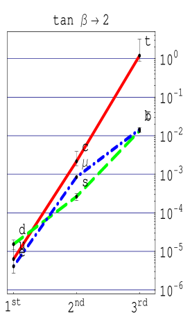
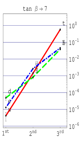
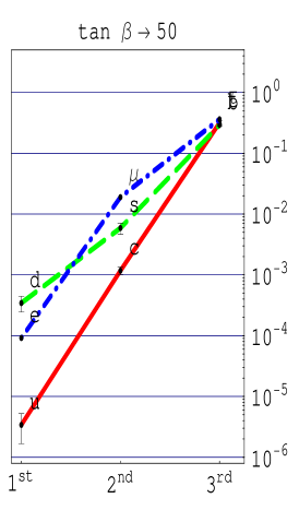
Figure 3: Yukawa couplings at GUT scale calculated from experimental charged fermions masses, assuming MSSM running and including uncertainty from experiments and from $\lambda_{t}$ renormalization. U, D, E are respectively red (continuous), green (dashed) and blue (dot-dashed).

4 SO(10) realizations

To realize these three models of Yukawa couplings, for generic $n$, one should look for effective heavy fermion mass operators of the form,

$$M_{\rm heavy}^{ij}\propto\bigg{(}\frac{\mathbf{1}_{X}}{\mathbf{45}_{X}}\bigg{)}^{\!n}\,\bigg{[}\chi^{ij}_{1}\,+\frac{\mathbf{45}_{X}}{{\mathbf{1}_{X}}}\,\chi^{ij}_{2}\,+\frac{\mathbf{45}_{X}^{\!2}}{{\mathbf{1}_{X}}^{2}}\,\chi^{ij}_{3}\bigg{]}\,,$$ (37)

where again the $\chi^{ij}_{1,2,3}$ are sextets of flavour with VEV that gives the $\hat{Q}_{1,2,3}$ projectors, and $\mathbf{1}_{X}$ is a singlet of SO(10)$\times$SU(3) with VEV larger than $M_{\rm GUT}$. Equivalently one may try to directly generate the light Yukawa couplings as effective operators of the form

$$\lambda_{ij}\propto\frac{\mathbf{45}_{R}}{{\mathbf{1}_{X}}^{2}}\bigg{(}\frac{\mathbf{45}_{X}}{{\mathbf{1}_{X}}}\bigg{)}^{\!n-2}\,\bigg{[}\frac{\mathbf{45}_{X}^{\!2}}{{\mathbf{1}_{X}}^{2}}\,\xi_{ij}^{1}\,+\frac{\mathbf{45}_{X}}{{\mathbf{1}_{X}}}\,\xi_{ij}^{2}\,+\xi_{ij}^{3}\bigg{]}\,,$$ (38)

where the $\xi^{1,2,3}_{ij}$ are now antisextets of flavour and their VEV are the $\hat{P}_{1,2,3}$ projectors.

All these effective operators can be realized using just renormalizable interactions introducing additional fields, that vary for the different cases. In general one has to add additional fermion multiplets beyond the $\mathbf{16}^{\prime}$ $\overline{\mathbf{16}}^{\prime}$, that can be taken to be vector-like as well; they will be denoted as $\mathbf{16}^{\prime\prime}$, $\overline{\mathbf{16}}^{\prime\prime}$, $\mathbf{16}^{\prime\prime\prime}$, $\overline{\mathbf{16}}^{\prime\prime\prime}$, etc. We then allow couplings of all the vector-like fermions together, but for simplicity we couple the light multiplet $\mathbf{16}$ just with $\mathbf{16}^{\prime}$, $\overline{\mathbf{16}}^{\prime}$, to realize the universal seesaw. The coupling matrix can be illustrated as:

$$\begin{array}[t]{l|cccc|}&\mathbf{16}^{i}&\mathbf{16}^{\prime}_{i}&\mathbf{16}^{\prime\prime}&\ldots\\ \hline\cr\mathbf{16}^{j}&&\mathbf{10}&&\\ \cline{3-5}\cr\overline{}\mathbf{16}^{\prime}_{j}&\mathbf{45}_{R}&\!\vline\hfill&&\\ \overline{}\mathbf{16}^{\prime\prime}&&\!\vline\hfill&M_{f\!ull}&\\ \vdots&&\!\vline\hfill&&\\ \hline\cr\end{array}$$

and $M_{f\!ull}$ will contain all the renormalizable couplings with SO(10) or flavour fields such as $\mathbf{45}$, $\chi_{ij}$, that all develop a VEV around the GUT scale.

The condition to use the universal seesaw approximation is that the involved eigenvalues of $M_{f\!ull}$ are heavier than $\langle\mathbf{45}_{R}\rangle$; once this is assured, the mass matrix $\hat{M}_{\rm heavy}$ of the heavy states is effectively given by the projection of $M_{f\!ull}^{-1}$ into the $3\times 3$ subspace of the $\mathbf{16}^{\prime}_{i}$, $\overline{\mathbf{16}}^{\prime}_{j}$:

$$\hat{\lambda}\simeq\langle\mathbf{45}_{R}\rangle\hat{M}_{\rm heavy}^{-1}=\langle\mathbf{45}_{R}\rangle\,(\mathbf{1},0,\ldots)\,M_{f\!ull}^{-1}\raisebox{-16.00008pt}{$\left(\begin{array}[]{c}\mathbf{1}\\ 0\\ \vdots\end{array}\right)$}$$ (39)

where $\mathbf{1}$ stands for the identity in flavour space, $\delta_{ij}$. This means that to describe in the general case the resulting Yukawa couplings it is not necessary to diagonalize the entire coupling matrix, but it is sufficient to find the first 3$\times$3 block of the inverse of $M_{f\!ull}$.

In the following we describe some of the realizations of the Yukawa couplings (38) for the interesting cases $n=0,1,2$, introducing the additional fermion multiplets and the appropriate flavon fields.

4.1 Model I: first family unification, $n=0$

For $n=0$ the three terms appearing in $\hat{\lambda}$ have negative powers, 0, -1, -2, of $\mathbf{45}_{X}/{\mathbf{1}_{X}}$. These can be realized by introducing three more vector-like fermion multiplets that are flavour triplets, $\mathbf{16}^{\prime\prime\,i}_{1,2,3}$ (with their SO(10) conjugates $\overline{\mathbf{16}}^{\prime\prime\,i}_{1,2,3}$) and arranging the couplings as follows:

$$\begin{array}[t]{l|ccccc|}&\mathbf{16}^{i}&\mathbf{16}^{\prime}_{i}&\mathbf{16}^{\prime\prime\,i}_{1}&\mathbf{16}^{\prime\prime\,i}_{2}&\mathbf{16}^{\prime\prime\,i}_{3}\\ \hline\cr\mathbf{16}^{j}&&\mathbf{10}&&&\\ \overline{}\mathbf{16}^{\prime}_{j}&\mathbf{45}_{R}&&{\mathbf{1}_{X}}&{\mathbf{1}_{X}}&\mathbf{45}_{X}\\ \overline{\mathbf{16}}^{\prime\prime\,j}_{1}&&{\mathbf{1}_{X}}&\xi^{1}_{ij}&&\\ \overline{\mathbf{16}}^{\prime\prime\,j}_{2}&&\mathbf{45}_{X}&&\xi^{2}_{ij}&\\ \overline{\mathbf{16}}^{\prime\prime\,j}_{3}&&\mathbf{45}_{X}&&&\xi^{3}_{ij}\\ \hline\cr\end{array}$$

where $\xi^{1,2,3}$ are three flavour (anti)sextets. The effective $\hat{\lambda}_{f}$ of (38) emerges here from a double seesaw mechanism [19], and the VEVs of $\xi_{ij}^{1,2,3}$ directly generates the rank-one flavour projectors: $\hat{P}_{1,2,3}\propto\langle\xi^{1,2,3}\rangle$. Equivalently the $\hat{M}_{\rm heavy}$ mass matrix of (37) and the $\hat{Q}_{1,2,3}$ projectors can be seen to emerge from the first 3$\times$3 block of the inverse of $M_{f\!ull}$.

Such realization is not unique, for example one may realize the same effective operators in a more symmetric fashion with less fields, by introducing just two vector-like triplets and antitriplets $\mathbf{16}^{\prime\prime}_{i}$, $\overline{\mathbf{16}}^{\prime\prime}_{i}$, $\mathbf{16}^{\prime\prime i}$, $\overline{\mathbf{16}}^{\prime\prime i}$ along with three sextets $\chi_{n}^{ij}$, with couplings as follows:

$$\begin{array}[t]{l|cccc|}&\mathbf{16}^{i}&\mathbf{16}^{\prime}_{i}&\mathbf{16}^{\prime\prime}_{i}&\mathbf{16}^{\prime\prime i}\\ \hline\cr\mathbf{16}^{j}&&\mathbf{10}&&\\ \overline{\mathbf{16}}^{\prime}_{j}&\mathbf{45}_{R}&\chi_{1}^{ij}&\frac{1}{2}\chi_{2}^{ij}&\mathbf{45}_{X}\\ \overline{\mathbf{16}}^{\prime\prime}_{j}&&\frac{1}{2}\chi_{2}^{ij}&\chi_{3}^{ij}&{\mathbf{1}_{X}}\\ \overline{\mathbf{16}}^{\prime\prime\,j}&&\mathbf{45}_{X}&{\mathbf{1}_{X}}&\\ \hline\cr\end{array}$$

In this realization the VEV of the $\chi_{1,2,3}$ sextets gives the inverse flavour projectors that appear in $\hat{M}_{\rm heavy}$: i.e. $\hat{Q}_{1,2,3}\propto\langle\chi_{1,2,3}\rangle$ in (37). Then, the final $\hat{\lambda}_{f}$ will still be given as a combination of $\hat{P}_{1,2,3}$ as from the inversion property (18).

The coupling arrangments above, and the ones that will follow, are not the most general ones with the given fields: while some zeroes are motivated by SU(3) flavour symmetry or by SO(10), some other choices require a further explanation (for example the choice between $\mathbf{45}_{X}$ or ${\mathbf{1}_{X}}$). This may be linked to the presence of some additional symmetry (e.g. Z₃) that acts differently on the fields, or in the intertwining of gauge and flavour symmetries in a larger group. While these directions of investigation are very interesting, they go beyond the scope of the present work.

4.2 Model II: second family unification, $n=1$

For the case $n=1$, we describe first the realization using three triplets, that are equivalent to three sextets with rank-one VEV. One looks for a heavy mass $\hat{M}_{\rm heavy}$ of the form

$$\hat{M}_{\rm heavy}\propto\bigg{[}\frac{{\langle\mathbf{1}_{X}\rangle}}{\langle\mathbf{45}_{X}\rangle}\hat{Q}_{1}\,+\hat{Q}_{2}\,+\frac{\langle\mathbf{45}_{X}\rangle}{{\langle\mathbf{1}_{X}\rangle}}\hat{Q}_{3}\bigg{]}\,,$$ (40)

We parametrize the three sextets $Q_{1,2,3}^{ij}$ as before via the tensor product of three triplets: $\hat{Q}_{n}\propto q_{n}\,{q}_{n}^{t}$, with the $q_{n}$ the VEV of three flavour triplets scalar fields. Then the effective light Yukawa matrix can be realized by introducing four more vector-like fermion multiplets that are flavour singlets: $\mathbf{16}^{\prime\prime}_{1}$, $\mathbf{16}^{\prime\prime}_{2}$, $\mathbf{16}^{\prime\prime}_{3}$ and $\mathbf{16}^{\prime\prime\prime}$ (and their conjugates) and arranging the couplings as follows:

$$\begin{array}[t]{l|cccccc|}&\mathbf{16}^{i}&\mathbf{16}^{\prime}_{i}&\mathbf{16}^{\prime\prime}_{1}&\mathbf{16}^{\prime\prime}_{2}&\mathbf{16}^{\prime\prime}_{3}&\mathbf{16}^{\prime\prime\prime}\\ \hline\cr\mathbf{16}^{i}&&\mathbf{10}&&&&\\ \overline{}\mathbf{16}^{\prime}_{j}&\mathbf{45}_{R}&&q_{1}&q_{2}&q_{3}&0\\ \overline{}\mathbf{16}^{\prime\prime}_{1}&&q_{1}&\mathbf{45}_{X}&&&\\ \overline{}\mathbf{16}^{\prime\prime}_{2}&&q_{2}&&{\mathbf{1}_{X}}&&\\ \overline{}\mathbf{16}^{\prime\prime}_{3}&&q_{3}&&&&{\mathbf{1}_{X}}\\ \overline{}\mathbf{16}^{\prime\prime\prime}&&0&&&{\mathbf{1}_{X}}&\mathbf{45}_{X}\\ \hline\cr\end{array}$$

By inverting in the vector-like sector the mass matrix $M_{f\!ull}$ and projecting in the $\mathbf{16}^{\prime}_{i}$, $\overline{\mathbf{16}}^{\prime}_{j}$ space one can see that the above form of $\hat{M}_{\rm heavy}$ is reproduced, inverted. Therefore, via the universal seesaw, one obtains in the light sector the correct Yukawa matrices:

$$\hat{\lambda}\propto\bigg{[}\frac{\langle\mathbf{45}_{X}\rangle}{\langle\mathbf{1}_{X}\rangle}p_{1}p_{1}^{t}\,+p_{2}p_{2}^{t}+\frac{\langle\mathbf{1}_{X}\rangle}{\langle\mathbf{45}_{X}\rangle}\,p_{3}p_{3}^{t}\bigg{]}\qquad\qquad f=u,d,e,\nu_{D}$$ (41)

i.e. $\hat{P}_{n}\propto p_{n}p_{n}^{t}$, with the reciprocal vectors defined again as $p_{n}=\frac{1}{2}\epsilon_{mnr}q_{n}\wedge q_{r}/(q_{1}\cdot q_{2}\wedge q_{3})$ (as from the inversion property (18)).

It is interesting to note that the way to obtain direct and inverse powers of $\mathbf{45}_{X}/{\mathbf{1}_{X}}$ together is that the first two channels $\mathbf{16}^{\prime\prime}_{1}$, $\mathbf{16}^{\prime\prime}_{2}$ are realizing a “double” seesaw, while the third $\mathbf{16}^{\prime\prime}_{3}$ a “triple” one. For we stress however that in the full seesaw the three rank-1 contributions work together, to reproduce the three terms in $\hat{\lambda}$.

One can also note that the scale of the ${q}_{1,2,3}$ triplets can be raised above the $\mathbf{45}_{X}$ scale and the double and triple seesaws still work as before. In the double seesaw this can be seen by comparing the determinant of the 2-3 block with that of the full matrix. A similar but more involved mechanism works for the triple seesaw. Indeed the next-to-smallest eigenvalues are, in the three cases, ${q}_{1}$,  ${q}_{2}^{2}/{\mathbf{1}_{X}}$ and $\mathbf{45}_{X}$. In the third case this is valid when ${q}_{n}\geq{\mathbf{1}_{X}}>\mathbf{45}_{X}$. Assuming then ${q}_{n}\geq{\mathbf{1}_{X}}>\mathbf{45}_{X}\simeq M_{\rm GUT}$, one can obtain that no mass eigenvalue, apart from the light fermion masses, drops below $M_{\rm GUT}$, so there will be no thresholds to take into account below the GUT scale. For this to happen, the scale of flavour breaking will be higher not only of the SO(10) breaking scale, but also of the higher ${\mathbf{1}_{X}}$ scale.

Other realizations of this model can be built by using antisextets or, for example, two triplets $q_{1,2}$ and one sextet $\chi_{3}$: for this one must introduce three vector-like fermion fields: two flavour singlets $\mathbf{16}^{\prime\prime}_{1,2}$ and one triplet $\mathbf{16}^{\prime\prime\prime i}$ (and their SO(10)$\times$SU(3) conjugates) and arranging the couplings as follows:

$$\begin{array}[t]{l|ccccc|}&\mathbf{16}^{i}&\mathbf{16}^{\prime}_{i}&\mathbf{16}^{\prime\prime}_{1}&\mathbf{16}^{\prime\prime}_{2}&\mathbf{16}^{\prime\prime\prime\,i}\\ \hline\cr\mathbf{16}^{j}&&\mathbf{10}&&&\\ \overline{}\mathbf{16}^{\prime}_{j}&\mathbf{45}_{R}&&q_{1}&q_{2}&\mathbf{45}_{X}\\ \overline{}\mathbf{16}^{\prime\prime}_{1}&&q_{1}&\mathbf{45}_{X}&&\\ \overline{}\mathbf{16}^{\prime\prime}_{2}&&q_{2}&&{\mathbf{1}_{X}}&\\ \overline{}\mathbf{16}^{\prime\prime\prime}_{j}&&\chi_{3}^{ij}&&&{\mathbf{1}_{X}}\\ \hline\cr\end{array}$$

The $\hat{Q}_{1,2,3}$ projectors appearing in the effective operator will be given by $\hat{Q}_{1}\propto q_{1}q_{1}^{t}$, $\hat{Q}_{2}\propto q_{2}q_{2}^{t}$ and $\hat{Q}_{3}\propto\chi_{3}$. Then the $\hat{P}_{1,2,3}$ projectors entering the light Yukawa matrices will be given again by the inversion formula (18).

4.3 Model III: third family unification, $n=2$

The third case corresponds to the popular but troublesome unification of the third family quarks and leptons. It requires very large $\mathop{\rm tan}\beta$ that is currently disfavored, and also involves a nonlinearity also from the renormalization evolution of the large $\lambda_{b}$ Yukawa eigenvalue, as well as more evident corrections to the $b$ mass [20]. For these reasons we will not pursue the analysis of its phenomenological viability: we will just give an example of a possible realization of the effective operator in this last case.

For $n=2$ we look for a realization of the following effective operator:

$$\hat{M}_{\rm heavy}\propto\bigg{[}\frac{{\langle\mathbf{1}_{X}\rangle}^{\!2}}{\langle\mathbf{45}_{X}^{\!2}\rangle}q_{1}q_{1}^{t}\,+\frac{{\langle\mathbf{1}_{X}\rangle}}{\langle\mathbf{45}_{X}\rangle}q_{2}q_{2}^{t}\,+q_{3}q_{3}^{t}\bigg{]}\,,$$ (42)

for which one is led to use a “triple” seesaw in all the three channels, by introducing for example six new flavour singlets multiplets $\mathbf{16}_{1,2,3}^{\prime\prime}$, $\mathbf{16}_{1,2,3}^{\prime\prime\prime}$ (and their vector-like conjugates), with the following couplings:

$$\begin{array}[c]{l|cccccccc|}&\mathbf{16}^{i}&\mathbf{16}^{\prime}_{i}&\mathbf{16}^{\prime\prime}_{1}&\mathbf{16}^{\prime\prime}_{2}&\mathbf{16}^{\prime\prime}_{3}&\mathbf{16}^{\prime\prime\prime}_{1}&\mathbf{16}^{\prime\prime\prime}_{2}&\mathbf{16}^{\prime\prime\prime}_{3}\\ \hline\cr\mathbf{16}^{j}&&\mathbf{10}&&&&&&\\ \overline{}\mathbf{16}^{\prime}_{j}&\mathbf{45}_{R}&&q_{1}&q_{2}&q_{3}&&&\\ \overline{}\mathbf{16}^{\prime\prime}_{1}&&q_{1}&&&&\mathbf{45}&&\\ \overline{}\mathbf{16}^{\prime\prime}_{2}&&q_{2}&&&&&{\mathbf{1}_{X}}&\\ \overline{}\mathbf{16}^{\prime\prime}_{3}&&q_{3}&&&&&&{\mathbf{1}_{X}}\\ \overline{}\mathbf{16}^{\prime\prime\prime}_{1}&&&\mathbf{45}&&&{\mathbf{1}_{X}}&&\\ \overline{}\mathbf{16}^{\prime\prime\prime}_{2}&&&&\mathbf{45}&&&{\mathbf{1}_{X}}&\\ \overline{}\mathbf{16}^{\prime\prime\prime}_{3}&&&&&{\mathbf{1}_{X}}&&&{\mathbf{1}_{X}}\\ \hline\cr\end{array}$$

5 Unification of determinants

Case II above, with $n=1$, is particularly interesting since it leads to an intriguing relation between Yukawa couplings. Looking at the determinant of the $\hat{\lambda}_{f}$ matrices, it turns out to factorize as:

$$\det\hat{\lambda}_{f}\;=\;\lambda^{3}\,D_{p}^{2}\,,$$ (43)

with $D_{p}=p_{1}\cdot(p_{2}\wedge p_{3})$. This expression is independent of $\epsilon_{f}$, and this means that the determinants are unified among the four U, D, E, $\nu_{D}$ sectors. In other words, at GUT scale the eigenvalues will satisfy the following exact relation:

$$\lambda_{e}\,\lambda_{\mu}\,\lambda_{\tau}=\lambda_{d}\,\lambda_{s}\,\lambda_{b}=\lambda_{u}\,\lambda_{c}\,\lambda_{t}=\lambda_{\nu_{D1}}\,\lambda_{\nu_{D2}}\,\lambda_{\nu_{D3}}\,.$$ (44)

The symmetry structure encoded in the generation of the Yukawa matrices, for case II, ensures that this relation is satisfied at GUT scale independently of the model parameters and details such as the pattern of breaking in the flavour and gauge sectors.

Obviously to rephrase (44) as relations between fermion masses at the weak scale one has to take into account the RG running, and this reintroduces a dependence on the model details, the value of $\alpha_{3}|_{Z}$, and mainly on the supersymmetry breaking scale.

To test the consequences of (44) on the low energy masses we recall that, in the MSSM, fermion masses and mixing angles are defined as follows in terms of quantities at the GUT scale:

$$\begin{array}[b]{lllll}m_{u}=\lambda_{u}v\sin\beta\,\eta_{uds}R_{u}B_{t}^{3}&&m_{d}=\lambda_{d}v\cos\beta\,\eta_{uds}R_{d}&&m_{e}=\lambda_{e}v\cos\beta\,\eta_{e\mu}R_{e}\\[4.30554pt] m_{c}=\lambda_{c}v\sin\beta\,\eta_{c}R_{u}B_{t}^{3}&&m_{s}=\lambda_{s}v\cos\beta\,\eta_{uds}R_{d}&&m_{\mu}=\lambda_{\mu}v\cos\beta\,\eta_{e\mu}R_{e}\\[4.30554pt] m_{t}=\lambda_{t}v\sin\beta\,\eta_{t}R_{u}B_{t}^{6}&&m_{b}=\lambda_{b}v\cos\beta\,\eta_{b}R_{d}B_{t}&&m_{\tau}=\lambda_{\tau}v\cos\beta\,\eta_{\tau}R_{e}\end{array}$$ (48)

$$\theta_{12}|_{Z}=\theta_{12}\,,\qquad\theta_{13}|_{Z}=\theta_{12}\,B_{t}^{-1}\,,\qquad\theta_{23}|_{Z}=\theta_{12}\,B_{t}^{-1}\,,$$ (49)

where: the factors $R_{u,d,e}$ account for the running induced by the MSSM gauge sector, from $M_{\rm GUT}$ to $m_{t}$; the factor $B_{t}$ accounts for the running induced by the large $\lambda_{t}$; and $\eta_{e\mu,uds,b,c}$ complete the QCD+QED running from $m_{t}$ down to $2\,\mbox{GeV}$ for $u$, $d$, $s$ or to the respective masses for $b$, $c$.

From [21], assuming $\alpha_{3}|_{Z}=0.118$ and $M_{\rm SUSY}=m_{t}$, we find

$$\eta_{uds}=1.74\,,\quad\eta_{c}=2.11\,,\quad\eta_{b}=1.52\,,\quad\eta_{\tau}=1.04\,,\quad\eta_{e\mu}=1.06\,,\quad\eta_{t}=1\,.$$ (50)

Then, we calculate

$$R_{u}=3.45\,,\qquad R_{d}=3.36\,,\qquad R_{e}=1.51\,,\qquad R_{\nu_{D}}=1.39\,.$$ (51)

The dependence on $\alpha_{3}|_{Z}$ of all these coefficients affects mainly the lightest quarks via $\eta_{uds}$, $\eta_{c}$ (10%), all the others have a variation of the order of 1-3%. These uncertainties are however correlated. In the $R_{u,d}$ factors there is also a stronger dependence on the supersymmetry breaking scale.

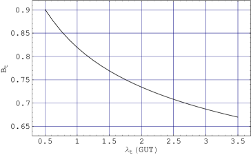
Figure 4: $B_{t}$ as a function of $\lambda_{t}$.

Finally, the factor $B_{t}$ is a function of $\lambda_{t}$, encoding the nonlinearity in the “top” renormalization due to its near Pendleton-Ross supersymmetric fixed point. We obtain $B_{t}|_{\lambda_{t}\!=\!0.5}=0.901$, $B_{t}|_{\lambda_{t}\!=\!3.5}=0.670$. Near lower $\lambda_{t}$ the dependence on $\lambda_{t}$ is stiffer, and in power 6 it allows a quite precise determination of $\lambda_{t}$ from the experimental value of $m_{t}$. Indeed, one can estimate the factor $B_{t}$ after determining $\lambda_{t}$ from $m_{t}$, once one notices that $m_{t}$ is almost independent of $\mathop{\rm tan}\beta$ in its moderate range, i.e. $\sin{\beta}\simeq 0.99$ within 0.5%, and that $\lambda_{t}$ turns out to lie near 0.5, so that $B_{t}$ is sufficiently dependent of $\lambda_{t}$. Taking into account the uncertainty in $m_{t}$ one finds $\lambda_{t}=0.536\mbox{--}0.809$ and $B_{t}=0.8734\pm 2.5\%_{m_{t}}$.

At this point, identities (44) can be rewritten in the following form involving only low energy fermion masses:

$$m_{d}m_{s} = \frac{m_{e}m_{\mu}m_{\tau}}{m_{b}}\,\frac{R_{d}^{3}\eta_{b}\eta_{uds}^{2}}{R_{e}^{3}\eta_{e\mu}^{2}\eta_{\tau}}B_{t}$$ (52)

$$m_{u} = \frac{m_{e}m_{\mu}m_{\tau}}{m_{c}m_{t}}\,\frac{R_{u}^{3}\eta_{c}\eta_{uds}}{R_{e}^{3}\eta_{e\mu}^{2}\eta_{\tau}}(\mathop{\rm tan}\beta)^{3}B_{t}^{12}$$ (53)

and this implies the following predictions for $m_{d}m_{s}$ and $m_{u}$:

$$m_{d}m_{s} = 880\,\mbox{MeV}^{2}\pm 2\%_{m_{t}}\pm 4\%_{m_{b}}\pm 25\%_{\alpha_{3}}$$ (54)

$$m_{u} = \bigg{(}\frac{\mathop{\rm tan}\beta}{7}\bigg{)}^{3}1.95\,\mbox{MeV}\pm 20\%_{m_{t}}\pm 10\%_{m_{c}}\pm 15\%_{\alpha_{3}}\,.$$ (55)

Using a mean value of 19.5 for the known ratio $m_{s}/m_{d}$, the first equation gives the central values

$$m_{d}=6.7\,\mbox{MeV}\,,\qquad m_{s}=131\,\mbox{MeV}\,,$$ (56)

that fit well the data, with $m_{s}$ a bit high, within 1$\sigma$ of the experimental range. This means that experimentally the D, E determinants are unified at GUT scale within 1-$\sigma$.

The prediction for $m_{u}$ carries a dependence on $\mathop{\rm tan}\beta$, that can be used to derive a prediction for it:

$$\mathop{\rm tan}\beta=7.3\,\pm 1.3_{m_{u}}\,\pm 0.5_{m_{t}}\,\pm 0.2_{m_{c}}\,,$$ (57)

where we used the 1$\sigma$ range for $m_{u}=(3\pm 1.5)\,\mbox{MeV}$ [22]. This prediction lies exactly in the favored range determined from the recent analysis in various MSSM scenarios [22, 18].

An other prediction for $\mathop{\rm tan}\beta$ may be derived by combining the two above and assuming for $m_{u}/m_{d}$ and $m_{s}$ their experimental ranges. One gets:

$$\mathop{\rm tan}\beta = \bigg{(}\frac{m_{u}}{m_{d}}\,\frac{m_{c}m_{t}}{m_{s}m_{b}}\bigg{)}^{1/3}\frac{R_{u}}{R_{d}}\bigg{(}\frac{\eta_{b}\eta_{uds}}{\eta_{c}}\bigg{)}^{1/3}B_{t}^{-11/3}$$ (58)

$$= 10\,\pm 1.3_{m_{u}/m_{d}}\,\pm 1_{m_{s}}\,\pm 1_{m_{t}}\,\pm 0.5_{\alpha_{3}}\,.$$

Of course this prediction tells what is the value of $\mathop{\rm tan}\beta$ once the model has been solved and $m_{u}/m_{d}$, $m_{s}$ and $m_{t}$ are determined. However we have found that the dependence on $\alpha_{3}|_{Z}$ cancels almost perfectly in both the ratios involving the $R$’s and the $\eta$’s, and enters only through the $B_{t}$ dependence ($<\!4\%$). This is a remarkable fact, considering that for individual masses the uncertainty in $\alpha_{s}|_{Z}$ generates the dominant errors in their predictions.

In addition, and equally remarkably, the even larger dependence on the supersymmetry breaking scale also cancels almost exactly in the ratio $R_{u}/R_{d}$, and enters just through the $B_{t}$ factor, where it can be estimated as a small decrease of 3% when $M_{\rm SUSY}$ is raised from $167\,\mbox{GeV}$ to $1\,\mbox{TeV}$.

6 Model analysis

One may take the decomposition in rank-one projectors described until here as an ansatz, and verify that it can explain all fermion masses and mixing angles. To this aim we will write the mass matrices in terms of a number of independent parameters, and show how to determine them from the known masses, mixing angles, and CP violation phase.

First of all let us parametrize the symmetric flavour projectors $\hat{P}_{n}$ in terms of the three triplets $p_{n}$, and choose a flavour basis to write the projectors as follows:

$$\hat{\lambda}_{f}=\lambda\Big{[}\epsilon_{f}\hat{P}_{1}\,+\hat{P}_{2}\,+\epsilon_{f}^{-1}\hat{P}_{3}\Big{]} = \lambda\left[\epsilon_{f}\left(\begin{array}[]{ccc}1&a&b\\ a&a^{2}&ab\\ b&ab&b^{2}\end{array}\right)+\left(\begin{array}[]{ccc}0&0&0\\ 0&1&c\\ 0&c&c^{2}\end{array}\right)+\epsilon_{f}^{-1}\left(\begin{array}[]{ccc}0&0&0\\ 0&0&0\\ 0&0&d^{2}\end{array}\right)\right]$$ (68)

$$= \lambda\left(\begin{array}[]{ccc}\epsilon_{f}&a\,\epsilon_{f}&b\,\epsilon_{f}\\[4.30554pt] a\,\epsilon_{f}&1+a^{2}\epsilon_{f}&c+ab\,\epsilon_{f}\\[4.30554pt] b\,\epsilon_{f}&c+ab\,\epsilon_{f}&d^{2}/\epsilon_{f}+c^{2}+b^{2}\epsilon_{f}\end{array}\right)\,,$$ (72)

where we have rotated globally all the $p_{n}$ vectors in flavour space and rescaled $\epsilon_{f}$, $\lambda$ to set $p_{1}=(1,a,b)$, $p_{2}=(0,1,c)$, $p_{3}=(0,0,d)$. Eliminating also the irrelevant phases, we end up with the following 15 parameters domain: $\lambda,a,d\in{\mathbb{R}}^{+}$, $b,c,\epsilon_{u},\epsilon_{d},\epsilon_{e},\epsilon_{\nu_{D}}\in{\mathbb{C}}$. Because of the SO(10) relations (33) two $\epsilon$ may be eliminated and we remain with 11 real parameters. This form should account for all the Dirac couplings of charged fermions and neutrinos.

For the Majorana mass matrix of neutrinos, in view of (35), we have a similar form, but involving $\epsilon_{\nu_{L}}$ in place of $\epsilon_{f}$ and with $\alpha$ appearing in the $d^{2}/\epsilon_{\nu_{L}}$ term in the 3-3 entry. The neutrino sector thus adds 4 real parameters to the model.

6.1 Leading order

The yukawa sector can be analyzed quite completely by computing the leading order expressions for eigenvalues and mixing angles. For charged fermions:

$$\lambda_{u}\simeq\lambda\,|\epsilon_{u}|\,,\ \ \qquad\quad \lambda_{c}\simeq\lambda\,,\quad\ \ \ \ \ \ \qquad\qquad\lambda_{t}\simeq\lambda\left|\frac{d^{2}}{\epsilon_{u}}\right|$$ (73)

$$\lambda_{d}\simeq\lambda\frac{|\epsilon_{d}|}{|1+{a^{2}\epsilon_{d}}|}\,,\quad \lambda_{s}\simeq\lambda|1+{a^{2}\epsilon_{d}}|\,,\quad\qquad\lambda_{b}\simeq\lambda\left|\frac{d^{2}}{\epsilon_{d}}\right|$$ (74)

$$\lambda_{e}\simeq\lambda\frac{|\epsilon_{e}|}{|1+{a^{2}\epsilon_{e}}|}\,,\quad \lambda_{\mu}\simeq\lambda|1+{a^{2}\epsilon_{e}}|\,,\quad\qquad\lambda_{\tau}\simeq\lambda\left|\frac{d^{2}}{\epsilon_{e}}\right|$$ (75)

$$\theta_{12}\simeq-\frac{a\epsilon_{d}}{1+a^{2}\epsilon_{d}}\,,\qquad\theta_{23}\simeq\frac{\eta_{d}}{d^{2}}\epsilon_{d}\,,\qquad\theta_{13}\simeq\frac{b}{d^{2}}\epsilon_{d}^{2}\,,\qquad\gamma_{\rm CP}\simeq\arg\left(\frac{b(1+a^{2}\epsilon_{d})}{\eta_{d}}\right),$$ (76)

where $\eta_{d}=(c+ab\,\epsilon_{d})$. Note also that since $\epsilon_{u}\ll\epsilon_{d,e}$, the quark mixing angles are well approximated by the “down” sector. The analysis proceeds with the following steps:

• First we note from the third generation that, to respect $\lambda_{b}/\lambda_{\tau}\simeq 1$, one should have $|\epsilon_{e}|\simeq|\epsilon_{d}|$ as already discussed. This relation holds within 10%, but is nevertheless important for the following first order calculation.

• Then, if one notes that ignoring the corrections the second generation Yukawa are unified $\lambda_{c,s,\mu}\simeq\lambda$, on the other hand the RG invariant relation $s_{12}\simeq\sqrt{m_{d}/m_{s}}$ tells us that $|a^{2}\epsilon_{d}|\simeq 1$, so that $a$ should actually be quite large, $|a|\sim|\epsilon_{d}|^{-1/2}$ ($\simeq 7$, see later) and the corrections can not be neglected.

• On the contrary, one sees that the required split of s,$\mu$ Yukawa is produced by the factors $A_{d,e}=|1+a^{2}\epsilon_{d,e}|$ once the sign (the phases) of $a^{2}\epsilon_{e}$ and $a^{2}\epsilon_{d}$ are nearly opposite, $a^{2}\epsilon_{e}\simeq-a^{2}\epsilon_{d}\simeq\mbox{e}^{0.5i}$, so that $|A_{e}|\simeq 2$, $|A_{d}|\simeq 0.5$. For the first generation the split goes (correctly!) in the opposite direction. Therefore, in this approach, the largeness of $a$, following from the Cabibbo angle, explains also the deviation from exactly family hierarchical masses of $e$, $d$, $\mu$, $s$. This fact was observed in [7].

• From other known mass ratios one can then determine $|\epsilon_{e,d}|\simeq 1/55$, $a\simeq 7.5$, $|\epsilon_{u}|\simeq 1/600$, $d^{2}\simeq 0.5$, $\mathop{\rm tan}\beta\simeq 7.3$.

• Further insight can be gained by looking at the other quark mixing angles. From:

  $$\theta_{13}\simeq|b\,\epsilon_{d}^{2}/d^{2}|=3\cdot 10^{-3}\,,\qquad\theta_{23}\simeq|\eta_{d}\epsilon_{d}/d^{2}|=4\cdot 10^{-2}\,,$$ (77)

  where $\eta_{d}=(c+ab\,\epsilon_{d})$, one derives $|b|\simeq 5$, $|c|\simeq 0.5\mbox{--}1.5$. Therefore the consequences of $\theta_{13}$ are similar to the effect of the Cabibbo mixing: while there we got that numerically $a\simeq\epsilon_{d}^{-1/2}$, now we see that also $b\simeq\epsilon_{d}^{-1/2}$ is large, of the same order. This does not introduce significant correction to the third-generation eigenvalues but, below, will help neutrino to have a maximal atmospheric mixing.

• A phase can be determined from the CKM CP-violating phase $\gamma_{\rm CP}$:

  $$\gamma_{\rm CP}\simeq\arg\bigg{(}\frac{b(1+a^{2}\epsilon_{d})}{\eta_{d}}\bigg{)}=1.02\,,\quad\Longrightarrow\quad\arg(b)-\arg(\eta_{d})=1\pm 1=\Big{\{}\begin{array}[]{ll}0\\ 2\end{array}\,,$$ (78)

  where we had from the first two steps that $\arg(1+a^{2}\epsilon_{d})\simeq\pm 1$, the sign depending on complex conjugation of $\epsilon_{d}$. Fixing in this way the relative phase of $b$ with $\eta_{d}$ also fixes the modulus of $c=\eta_{d}-ab\,\epsilon_{d}$. The two branches correspond to $|c|\simeq 0.2$, $|c|\simeq 1.5$. In the first branch, $c$ and $b$ are approximately orthogonal, in the second they are approximately opposite.

• Two remaining free parameters can be taken to be $|\epsilon_{e}/\epsilon_{d}|$, $\arg c$, and one can be eliminated (using second order corrections to eigenvalues) from the precise ratio $\lambda_{b}/\lambda_{\tau}\simeq[|\epsilon_{e}/\epsilon_{d}|+2\mathop{\rm Re}(\epsilon_{d}c^{2}/d^{2})]$.

Summing up, the leading order analysis for charged fermions shows a one parameter family of solutions, with two branches. The flat direction can be taken as a combination of $|\epsilon_{e}/\epsilon_{d}|$ with the common phase of $b$, $c$.

The precise leading-order solution for all parameters is not conclusive since next-to-leading corrections and contributions to CKM from the “up” sector are 10% in magnitude, larger than experimental errors; hence a numeric fit is necessary and will be described below. Nevertheless the model proves capable of accounting for all the charged fermion masses and mixings, giving a mechanism for linking the deviations $A_{e,d}$ with the Cabibbo angle $\theta_{12}$.

We can now comment on the solution found from the charged fermions so far. Collecting the $p_{n}$ vectors:

$$p_{1}=(1,\,7,\,5)\,,\qquad p_{2}\simeq(0,\,1,\,0.2\mbox{--}1.5)\,, \qquad p_{3}\simeq(0,\,0,\,0.7)\,,$$ (79)

we observe that the they tend to lie in the 2-3 plane. Exact planarity is broken to order $1/8\simeq\sqrt{\epsilon_{d}}$, as can be seen from the first 1, with respect to the modulus of its vector $|p_{1}|\simeq 8.5$. The reason for this is to be tracked in the magnitude of the quark mixing angles that require $a$ and $b$ to be large while $c$ and $d$ are of order one. In terms of the reciprocal vectors $q_{1,2,3}$ that appear in the model II realization in section 4.2, quasi-planarity shows up as quasi-alignment. We have

$$q_{1}=(1,0,0)\,,\qquad q_{2}=(7,1,0)\,,\qquad q_{3}\simeq(7,1,1)\,.$$ (80)

We find this pattern of quasi-planar or quasi-aligned triplets a nice hint for the realization of in the flavour sector of the theory, where three flavour triplets scalar fields acquire a VEV that generates the $p_{n}$ vectors. We leave this possibility for future model building; see e.g. [15] for realizations of disoriented VEVs from a potential.

We observe also that if one may be concerned with the moduli of $p_{n}$ not being equal and of order 1, (they are in fact $|p_{1}|\simeq 8$, $|p_{2}|\simeq 1.5$, $|p_{3}|\simeq 0.7$), they can be brought to be in the range 1–2 by rescaling all the $\epsilon_{f}$ by a factor of 10. With this normalization the hierarchy of eigenvalues is due partially to the $\epsilon_{f}$ and partially to the $p_{n}$ vectors having hierarchic entries, while the normalization that we adopted above corresponds to an eigenvalue hierarchy that comes only from the $\epsilon_{f}$’s. The choice may be varied depending on the theoretical realization in the flavour sector, that should be the subject of a further study and goes beyond the scope of this work.

6.2 Neutrino analytical

From the light neutrino mass matrix (35) and using the explicit parametrization given in (68), we can rewrite:

$$\lambda_{\nu_{L}}\propto\left(\begin{array}[]{ccc}|\epsilon_{\nu}/\bar{A}_{\nu}|&|a\epsilon_{\nu}/A_{\nu}|&|b\epsilon_{\nu}/A_{\nu}|\\ |a\epsilon_{\nu}/A_{\nu}|&1&\hbox to0.0pt{$\rho$\hss}\mbox{\phantom{$\rho^{2}+\sigma$}}\\ |b\epsilon_{\nu}/A_{\nu}|&\rho&\rho^{2}+\sigma\end{array}\right).$$

with $A_{\nu}=(1+a^{2}\epsilon_{\nu})$,  $\rho=(c+ab\epsilon_{\nu})/A_{\nu}$,  $\sigma=(d^{2}\alpha+(b-ac)^{2}\epsilon_{\nu}^{2})/A_{\nu}$.

In this matrix, we only have two free complex parameters $\epsilon_{\nu}$ and $\alpha$, and the common phase of $b$, $c$ that was a flat direction of the charged fermions. However it is easy to see by homogeneity that this latter phase is irrelevant since it can be eliminated using the phase of $\alpha$. Therefore, we have just two complex parameters $\epsilon_{\nu}$ and $\alpha$, and also the neutrino sector is quite constrained.

Because of the large neutrino mixings and of the small but important uncertainties in the parameters determined from the charged fermions, an exact analytical decomposition of this matrix is quite difficult. Nevertheless some useful observations can be made:

• First, since the ratio of the 1-1 with the 1-2, 1-3 entries is small $\simeq 1/7$, from the known pattern of mixing angles it follows that this matrix predicts direct and non degenerate neutrinos: $m_{\nu 1}/m_{\nu 2}\simeq 1/4$ so that $m_{\nu 2}/m_{\nu 3}\simeq 1/5$.

• Then, because the 1-2 entry is larger than the 1-3 one (1-2/1-3 $\simeq 1.5$–2), then $\theta_{e3}$ cannot be zero.

• An estimate of the angles from the 2,3 sector can be given first in the form of a correlation between them, using the parameters found from the charged sector and after the requirement of maximal $\theta_{\rm atm}$:

  $$\frac{\theta_{e3}}{\theta_{\rm sol}}=\frac{m_{\nu 2}}{m_{\nu 3}}\,\Big{|}\frac{1+R\,{\rm e}^{i\delta}}{1-R\,{\rm e}^{i\delta}}\Big{|}\,,\qquad\mbox{with }\ R=\frac{b}{a}\simeq\frac{\theta_{13}^{\rm quark}\lambda_{b}}{\theta_{12}^{\rm quark}\lambda_{s}}\simeq\frac{1}{1.6\thicksim 2.1}\,,$$ (81)

  where $\delta=\arg\rho$. After imposing the correct neutrino hierarchy to solve for $\epsilon_{\nu}$, we can estimate more explicitly:

  $$\theta_{\rm sol}\simeq 30^{\circ}\Big{|}1-R\,{\rm e}^{i\delta}\Big{|}\,,\qquad\theta_{e3}\simeq 6^{\circ}\Big{|}1+R\,{\rm e}^{i\delta}\Big{|}\,.$$ (82)

  Therefore, choosing ${\rm e}^{i\delta}$ purely imaginary or just slightly negative, we see that the right $\theta_{\rm sol}\simeq 32^{\circ}$ is accommodated, with a prediction for $\theta_{e3}\simeq 5^{\circ}$.

  The precise numbers are sensible to the precise values of the quark mixing angles and CP-phase, as well as to the neutrino hierarchy. In practice $\theta_{e3}$ can be brought reach the extrema of the range $\theta_{e3}\simeq 1^{\circ}\mbox{--}7.5^{\circ}$, by stretching within 1$\sigma$ the angles and the neutrino hierarchy. This means that the model predicts a nonzero $\theta_{e3}$ inside the present 2$\sigma$ range (=0^∘–9.6^∘). With more precise experimental values of CKM angles and neutrino hierarchy, also the prediction for $\theta_{e3}$ will become narrower.

• Finally, it can be seen that among the four parameters a flat direction emerges, along which the angles and hierarchy do not vary. It directly corresponds to the leptonic CP violation phase, that is thus left unpredicted by this ansatz, until angles and hierarchy will be known to better accuracy. Also one Majorana phase varies along this flat direction.

Summing up, in the neutrino sector the model predicts hierarchic neutrinos with nonzero $\theta_{e3}$ in the present range, and there is a useful conspiracy from the charged fermions sector to allow the right neutrino pattern. A flat direction emerges as a combination of the four real parameters, and has to be added to the one found in the charged leptons sector. Therefore the whole model effectively takes advantage of just 13 of the 15 real parameters to reproduce the known data.

For a precise test we performed a numerical analysis, where we fitted neutrinos together with charged fermions. The $\theta_{e3}$ mixing, that we have shown to lie automatically inside its allowed range, will not be used as a fit parameter but rather displayed as a model prediction.

6.3 Numeric fit and results

The fit was performed using the 15 parameters (11 charged fermions, 4 neutrino) against 20 tests for all known data [22, 23]. The best fit results are shown in tables 1 and 2, for models I and II. Each model has solutions in two branches, and model I shows difficulties in fitting the “up” sector ($m_{t}$ is too low, and $m_{c}$ too high). Model II instead can fit almost perfectly all data, albeit predicting a bit low $m_{u}$ and a bit large $m_{s}$ as implied by the predictions described in section 5.

The dependence on the supersymmetry breaking scale is the major source of theoretical uncertainty, and we have estimated its effect by performing the fit also with $M_{\rm SUSY}=1\,\mbox{TeV}$ and including mixed RG evolution. Raising the SUSY scale leads to better results in both models, but more appreciably in model II where all tension with experimental data disappears, and unification of determinants works perfectly.

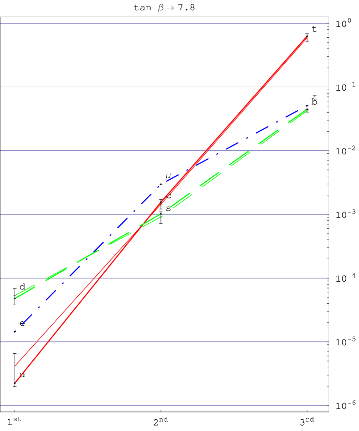
Figure 5: Illustration of yukawa couplings at GUT scale for the three families of charged fermions, resulting from the best fit in model II for $M_{\rm SUSY}=167\,\mbox{GeV}$, compared to the values calculated from experimental masses (as shown in figure 3). Thin lines connect yukawa calculated from experimental masses, thick lines correspond to the best fit result.

For model II we also illustrate the best fit Yukawa couplings in figure 5.

A number of observations from the fit results in model II can be made:

• Apart from $m_{u}$ and $m_{s}$ with lower $M_{\rm SUSY}$ that are predicted in the $1\sigma$ range, all data are accomodated without any tension. Within the same total deviation one may choose even to adjust better either $m_{s}$, $m_{u}/m_{d}$ or $m_{c}$ and $m_{t}$.

• A flat direction and the two branches $|c|\simeq 0.2,1.5$ correctly emerge from the fit. In the second branch all complex phases of all parameters are almost aligned, hinting for a model with aligned $\epsilon_{f}$’s and real parameters, with a reduction of the total number of real parameters to 10.

• In the lepton sector, the mixing from terrestrial neutrinos is nonzero: $\theta_{e3}\simeq 2^{\circ},6^{\circ}$, respectively in the two branches.

• Neutrino come out hierarchic and non degenerate $m_{\nu}\simeq(0.0045,\,0.01,\,0.048)\,\mbox{eV}$, and right-handed neutrino masses are of the order ($10^{7}$, $10^{9}$, $10^{11}$) GeV.

• The leptogenesys asymmetry appears to have the correct sign $\epsilon_{1}\simeq-3\cdot 10^{-9}$ at least in some branches, though (due to small RH neutrino masses) the value itself is too small for the usual thermal scenario, and it requires a specific assumption on the non-thermal production of the heavy neutrino initial abundances.

$\begin{array}[t]{|c|c||c|c||c|c|}\hline\cr\vrule\lx@intercol\hfil\mbox{MODEL I}\hfil\lx@intercol\vrule\lx@intercol\\ \hline\cr\vrule\lx@intercol\hfil\hfil\lx@intercol\vrule\lx@intercol\vrule\lx@intercol&\lx@intercol\hfil M_{\rm SUSY}=m_{t}\hfil\lx@intercol\vrule\lx@intercol\vrule\lx@intercol&\lx@intercol\hfil M_{\rm SUSY}=1\mbox{TeV}\hfil\lx@intercol\vrule\lx@intercol\\ &\mbox{exp}&\mbox{$1^{\rm st}$ branch}&\mbox{$2^{\rm nd}$ branch}&\mbox{$1^{\rm st}$ branch}&\mbox{$2^{\rm nd}$ branch}\\ \hline\cr\lx@intercol\hfil Fit\hfil\lx@intercol\\ \hline\cr m_{t}&167\pm 5&{\bf 147}&{\bf 148}&{\bf 155}&{\bf 155}\\ m_{b}&4.25\pm 0.15&4.36&4.38&4.37&4.37\\ m_{c}&1.25\pm 0.10&\ {\bf 1.49}&\ {\bf 1.47}&{\bf 1.46}&{\bf 1.45}\\ m_{s}&105\pm 25&{\bf 132}&119&128&116\\ m_{s}/m_{d}&19.5\pm 2.5&21.1&21&21.8&{\bf 22.2}\\ \mbox{Ellipse}&23\pm 2&22.1&22.6&22.5&22.9\\ m_{u}/m_{d}&0.5\pm 0.2&{\bf 0.26}&{\bf 0.27}&{\bf 0.26}&{\bf 0.25}\\ m_{u}\!\!+\!m_{d}&8.5\pm 2.5&7.6&8.0&7.3&6.5\\ \hline\cr\theta_{12}&12.7\pm 0.1&12.75&12.75&{\bf 12.81}&{\bf 12.83}\\ 10^{2}\,\theta_{23}&4.13\pm 0.15&4.11&4.12&4.11&4.12\\ 10^{3}\,\theta_{13}&3.67\pm 0.47&3.82&3.79&3.82&3.79\\ \sin\!2\beta_{\rm CP}&0.736\pm 0.05&0.735&0.734&0.730&0.734\\ \gamma_{\rm CP}&1.03\pm 0.22&0.93&1.05&0.93&1.02\\ \hline\cr\theta_{\rm sol}&32\pm 3&31.&32.&31.0&32.\\ \theta_{\rm atm}&45\pm 7&45.3&45.&45.3&45.\\ h_{\nu}&0.18\pm 0.07&0.165&0.180&0.171&0.185\\ \hline\cr\hline\cr\chi^{2}_{\rm dof}&&0.68&0.53&0.49&0.43\\ \hline\cr\lx@intercol\hfil Predictions\hfil\lx@intercol\\ \hline\cr m_{d}\,(\mbox{MeV})&6\pm 2&6.0&5.4&5.9&5.25\\ \theta_{e3}\,(^{\circ})&0\mbox{ -- }9.6&1.8&6.6&1.8&7.2\\ m_{\nu 1}\,(\mbox{eV})&&0.0029&0.0026&0.0029&0.0028\\ m_{\nu 3}\,(\mbox{eV})&&0.052&0.048&0.052&0.048\\ m_{ee}\,(\mbox{eV})&&0.0007&0.0009&0.0007&0.0009\\ \epsilon_{1}&&+2\,10^{-12}&+6\,10^{-12}&+2\,10^{-12}&+2.7\,10^{-12}\\ \hline\cr\mathop{\rm tan}\beta&&1.21&1.23&1.13&1.14\\ \hline\cr\end{array}$

Table 1: Result of best fit against the known experimental ranges, for the two branches of model I, varying also the supersymmetry breaking scale between the “top” scale $167\,\mbox{GeV}$ and $1\,\mbox{TeV}$. In bold are shown the quantities that show a $1\sigma$ tension with experiment. Lepton masses are reproduced exactly and are not displayed. We report also some predicted quantities, not used for fitting, but determined in the best fit solution. This model shows a evident difficulty in accommodating the “up” quark sector.

$\begin{array}[t]{|c|c||c|c||c|c|}\hline\cr\vrule\lx@intercol\hfil\mbox{MODEL II}\hfil\lx@intercol\vrule\lx@intercol\\ \hline\cr\vrule\lx@intercol\hfil\hfil\lx@intercol\vrule\lx@intercol\vrule\lx@intercol&\lx@intercol\hfil M_{\rm SUSY}=m_{t}\hfil\lx@intercol\vrule\lx@intercol\vrule\lx@intercol&\lx@intercol\hfil M_{\rm SUSY}=1\mbox{TeV}\hfil\lx@intercol\vrule\lx@intercol\\ &\mbox{exp}&\mbox{$1^{\rm st}$ branch}&\mbox{$2^{\rm nd}$ branch}&\mbox{$1^{\rm st}$ branch}&\mbox{$2^{\rm nd}$ branch}\\ \hline\cr\lx@intercol\hfil Fit\hfil\lx@intercol\\ \hline\cr m_{t}&167\pm 5&167.6&169.0&167.4&167.8\\ m_{b}&4.25\pm 0.15&4.40&4.45&4.32&4.38\\ m_{c}&1.25\pm 0.10&1.32&1.31&1.29&1.29\\ m_{s}&105\pm 25&{\bf 134}&{\bf 134}&127&126\\ m_{s}/m_{d}&19.5\pm 2.5&21.1&21.4&21.01&21.0\\ \mbox{Ellipse}&23\pm 2&21.5&22.1&21.46&22.2\\ m_{u}/m_{d}&0.5\pm 0.2&{\bf 0.20}&{\bf 0.25}&{\bf 0.21}&0.32\\ m_{u}\!\!+\!m_{d}&8.5\pm 2.5&7.5&8.0&7.3&7.9\\ \hline\cr\theta_{12}&12.7\pm 0.1&12.74&12.77&12.72&12.75\\ 10^{2}\,\theta_{23}&4.13\pm 0.15&4.12&4.14&4.11&4.13\\ 10^{3}\,\theta_{13}&3.67\pm 0.47&3.77&3.77&3.77&3.76\\ \sin\!2\beta_{\rm CP}&0.736\pm 0.05&0.730&0.734&0.73&0.734\\ \gamma_{\rm CP}&1.03\pm 0.22&0.97&1.07&0.98&1.06\\ \hline\cr\theta_{\rm sol}&32\pm 3&31.5&32.&31.4&32.\\ \theta_{\rm atm}&45\pm 7&45.1&45.&45.2&45.\\ h_{\nu}&0.18\pm 0.07&0.178&0.185&0.176&0.185\\ \hline\cr\hline\cr\chi^{2}_{\rm dof}&&0.30&0.27&0.22&0.14\\ \hline\cr\lx@intercol\hfil Predictions\hfil\lx@intercol\\ \hline\cr m_{d}\,(\mbox{MeV})&6\pm 2&6.4&6.3&6.1&6.0\\ \theta_{e3}\,(^{\circ})&0\mbox{ -- }9.6&2.1_{-0.4}^{+2.2}&6.4_{-5.5}^{+0.8}&1.9&5.9\\ m_{\nu 1}\,(\mbox{eV})&&0.0031&0.0030&0.0030&0.0044\\ m_{\nu 3}\,(\mbox{eV})&&0.050&0.048&0.050&0.0481\\ m_{ee}\,(\mbox{eV})&&0.00068&0.00091&0.0007&0.00085\\ \epsilon_{1}&&+3\,10^{-10}&-2\,10^{-9}&+2\,10^{-10}&-3.3\,10^{-9}\\ \hline\cr\mathop{\rm tan}\beta&&7.1_{-0.3}^{+0.5}&7.8_{-0.5}^{+0.5}&7.7&8.9\\ \hline\cr\end{array}$

Table 2: Result of best fit against the known experimental ranges, for the two branches of model II, varying the supersymmetry breaking scale between the “top” scale $167\,\mbox{GeV}$ and $1\,\mbox{TeV}$. In bold are shown the quantities that show a $1\sigma$ tension. For $\theta_{e3}$ and $\mathop{\rm tan}\beta$ we also indicate the ranges obtained, by stretching these quantities up to an additional 1$\sigma$ variation. It can be noted that raising the supersymmetry scale to $1\,\mbox{TeV}$ eliminates almost all tension, especially in the 2^nd branch.

7 Conclusions

We presented a predictive model of SU(3) flavour symmetry in the context of SO(10) supersymmetric GUT that can account for all the known fermion masses and mixings at less than 1$\sigma$ level, including neutrino data. The model has been analyzed with a leading-order analytical approach and with a complete numerical fit.

In the quark sector, it predicts 1$\sigma$ low $m_{u}$ and, without raising the SUSY breaking scale, 1$\sigma$ large $m_{s}$; all the other quantities are well accounted, including the CP phase. In the neutrino sector the model predicts direct and hierarchical neutrinos with non zero $\theta_{e3}\simeq 2^{\circ},6^{\circ}$ correlated to other quantities, but always within the present 99% c.l.. Also the correct sign of the leptogenesys asymmetry is an outcome of the numerical analysis, even though its magnitude is one or two orders of magnitude too low for the usual thermal leptogenesys scenario.

The SO(10) realization of this framework uses an “universal” seesaw mixing with superheavy vector-like fermions to transfer their mass matrices to the light fermions. Together with adjoint Higgs fields, it has been shown to suppress the dominant part of D=5 proton decay and supersymmetric flavour changing effects, while solving the doublet-triplet problem via the Missing VEV mechanism and allowing the correct mass generation.

The flavour structure of the model is based on hierarchical combinations of three rank-one projectors in flavour space, built with three flavour triplets or sextets, that break the SU(3) symmetry. As opposed to traditional unification schemes, this model does not unify some Yukawa matrices at GUT, but realizes in an interesting way the exact unification of their determinants.

A quite robust prediction for $\mathop{\rm tan}\beta\simeq 8$ in the moderate, favored, range is also consequence of this kind of unification.

The solution emerging from the analysis points to an interesting configuration of quasi-aligned flavour triplets, that suggests a precise pattern of SU(3) breaking. We leave this analysis for further work. Finally, the intertwining between flavour and SO(10) Higgs fields also suggests that a similar mechanism in the context of higher unification groups may lead to a framework as successful as this one.