Puzzles in $B\to\pi\pi,\pi K$ decays: Possible implications for R-parity violating supersymmetry

Abstract

Recent experiments suggest that certain data of $B\to\pi\pi,\pi K$ decays are inconsistent with the standard model expectations. We try to explain the discrepancies with R-parity violating suppersymmetry. By employing the QCD factorization approach, we study these decays in the minimal supersymmetric standard model with R-parity violation. We show that R-parity violation can resolve the discrepancies in both $B\to\pi\pi$ and $B\to\pi K$ decays, and find that in some regions of parameter spaces all these requirements, including the $CP$ averaged branching ratios and the direct $CP$ asymmetries, can be satisfied. Furthermore, we have derived stringent bounds on relevant R-parity violating couplings from the latest experimental data, and some of these constraints are stronger than the existing bounds.

PACS Numbers: 12.60.Jv, 12.15.Mm, 12.38.Bx, 13.25.Hw

1 Introduction

The detailed study of B meson decays plays an essential role for understanding the $CP$ violation and the physics of flavor. Recent experimental measurements [1, 2, 3, 4, 5, 6, 7, 8, 9, 10, 11, 12] have shown that some hadronic B decays to two pseudoscalar mesons deviate from the standard model (SM) expectations .

In the $B\to\pi\pi$ decays, there are three such discrepancies: the direct $CP$ asymmetry for the mode $B\to\pi^{+}\pi^{-}$ is very large [2, 10], the $\pi^{0}\pi^{0}$ mode is found to have a much larger branching ratio $(\approx 1.5\times 10^{-6})$ [4, 11] than the SM expectations $(\sim 10^{-7})$ [13, 14], and the theoretical estimation of $B\to\pi^{+}\pi^{-}$ branching ratio [13, 14] are about 2 times larger than the current experimental average [1, 7]. The “$B\to\pi\pi$ puzzle” is reflected by the following quantities [15]:

$$R^{\pi\pi}_{+-} \equiv 2\left[\frac{\mathcal{B}r(B^{+}\to\pi^{+}\pi^{0})+\mathcal{B}r(B^{-}\to\pi^{-}\pi^{0})}{\mathcal{B}r(B^{0}_{d}\to\pi^{+}\pi^{-})+\mathcal{B}r(\bar{B}^{0}_{d}\to\pi^{+}\pi^{-})}\right]\frac{\tau_{B_{d}}}{\tau_{B_{u}}}=(2.30\pm 0.35)_{exp},$$

$$R^{\pi\pi}_{00} \equiv 2\left[\frac{\mathcal{B}r(B^{0}_{d}\to\pi^{0}\pi^{0})+\mathcal{B}r(\bar{B}^{0}_{d}\to\pi^{0}\pi^{0})}{\mathcal{B}r(B^{0}_{d}\to\pi^{+}\pi^{-})+\mathcal{B}r(\bar{B}^{0}_{d}\to\pi^{+}\pi^{-})}\right]=(0.66\pm 0.14)_{exp},$$

here we use $\tau_{B_{u}}/\tau_{B_{d}}=1.069$ [16], the central values calculated within the QCD factorization (QCDF) give $R^{\pi\pi}_{+-}=1.24$ and $R^{\pi\pi}_{00}=0.07$ [13]. In Ref. [15], Buras et al. pointed out these data would indicate the large nonfactorizable contributions rather than new physics (NP) effects, and could be perfectly accommodated in the SM. However, it is hard to be realized by explicit theoretical calculations.

The $B\to\pi K$ system consists of the four decay modes $B^{0}_{d}\to\pi^{\pm}K^{\mp},B^{\pm}_{u}\to\pi^{\pm}K,B^{\pm}_{u}\to\pi^{0}K^{\pm}$ and $B^{0}_{d}\to\pi^{0}K^{0}$, which are governed by QCD penguin process $b\to sq\bar{q}$. The BABAR and Belle collaborations have measured the following ratios of the $CP$ averaged branching ratios [17]:

$$R \equiv \left[\frac{\mathcal{B}r(B^{0}_{d}\to\pi^{-}K^{+})+\mathcal{B}r(\bar{B}^{0}_{d}\to\pi^{+}K^{-})}{\mathcal{B}r(B^{+}\to\pi^{+}K^{0})+\mathcal{B}r(B^{-}\to\pi^{-}\bar{K}^{0})}\right]\frac{\tau_{B_{u}}}{\tau_{B_{d}}}=(0.79\pm 0.06)_{exp},$$

$$R_{c} \equiv 2\left[\frac{\mathcal{B}r(B^{+}\to\pi^{0}K^{+})+\mathcal{B}r(B^{-}\to\pi^{0}K^{-})}{\mathcal{B}r(B^{+}\to\pi^{+}K^{0})+\mathcal{B}r(B^{-}\to\pi^{-}\bar{K}^{0})}\right]=(0.98\pm 0.08)_{exp},$$

$$R_{n} \equiv \frac{1}{2}\left[\frac{\mathcal{B}r(B^{0}_{d}\to\pi^{-}K^{+})+\mathcal{B}r(\bar{B}^{0}_{d}\to\pi^{+}K^{-})}{\mathcal{B}r(B^{0}_{d}\to\pi^{0}K^{0})+\mathcal{B}r(\bar{B}^{0}_{d}\to\pi^{0}\bar{K}^{0})}\right]=(0.79\pm 0.08)_{exp},$$

where we have included the latest Belle [6] and BABAR [12] measurements. The ratio $R$, which is expected to be only marginally affected by color-suppressed electroweak (EW) penguins, does not show any anomalous behavior. The “$B\to\pi K$ puzzle” is reflected by the small value of $R_{n}$ which is significantly lower than $R_{c}$. Since $R_{c}$ and $R_{n}$ could be affected significantly by color-allowed EW penguins, the “$B\to\pi K$ puzzle” may be a manifestation of NP in the EW penguin sectors [15, 18, 19], and will offer an attractive avenue for physics beyond the SM to enter the $B\to\pi K$ system [20].

Although these measurements represent quite a challenge for theory, the SM is in no way ruled out yet since there are many theoretical uncertainties in low energy QCD. The recent theoretical results for $B\to\pi K$ [21, 22] show that the next to leading order corrections may be important. However, it will be under considerable strain if the experimental data persist for a long time. Existence of NP as possible solutions have been discussed in Refs. [15, 18, 23]. Among those NP models that survived EW data, one of the most respectable options is R-parity violating (RPV) supersymmetry (SUSY). The possible appearance of RPV couplings [24], which will violate the lepton and baryon number conservation, has gained full attention in searching for SUSY [25, 26]. The effect of RPV SUSY on B decays have been extensively investigated previously in the literatures [27, 28, 29, 30, 31, 32]. In this work, we extend our previous study of the $B\to VV$ decays [31] to the $B\to\pi\pi,\pi K$ decays using RPV SUSY theories by employing the QCD factorization (QCDF) approach[33] for hadronic dynamics. At the same theoretical ground, it would be interesting to know if we could find solutions to the $B\to\pi\pi$ and $B\to\pi K$ puzzles besides the $B\to VV$ polarization puzzle [31]. We show that the $B\to\pi\pi,\pi K$ puzzles could be resolved in the presence of the RPV couplings. Moreover, using the latest experimental data and theoretical parameters, we try to explain all available data including the $CP$ averaged branching ratios and the direct $CP$ asymmetries by the relevant RPV couplings. We note that the branching ratios of the $B\to\pi\pi,\pi K$ decays have also been studied in RPV SUSY in [32, 34]. In this study, we present a new calculation of the decays with up-to-date inputs, such as form factors, experimental measurements and so on.

The paper is arranged as follows. In Sec. II, we calculate the branching ratios and the $CP$ asymmetries of $B\to\pi\pi,\pi K$ decays, which contain the SM contributions and the RPV effects using the QCDF approach. In Sec. III, we tabulate theoretical inputs in our analysis. Section IV is to deal with data and discussions, we also display the allowed regions of the parameter space which satisfy all the experimental data. Section V contains our summary and conclusion.

2 The theoretical frame for $B\to\pi\pi$ and $\pi K$ decays

2.1 The decay amplitudes in the SM

In the SM, the low energy effective Hamiltonian for the $\Delta B=1$ transition at the scale $\mu$ is given by [35]

$$\mathcal{H}^{SM}_{eff} = \frac{G_{F}}{\sqrt{2}}\sum_{p=u,c}\lambda_{p}\Biggl{\{}C_{1}Q_{1}^{p}+C_{2}Q_{2}^{p}+\sum_{i=3}^{10}\Big{[}C_{i}Q_{i}+C_{7\gamma}Q_{7\gamma}+C_{8g}Q_{8g}\Big{]}\Biggl{\}}+h.c.,$$ (1)

here $\lambda_{p}=V_{pb}V_{pq}^{*}~{}(p\in\{u,c\})$ and the detailed definition of the operator base can be found in [35].

The decay amplitude for $B\to M_{1}M_{2}$ is

$$\mathcal{A}^{SM}(B\to M_{1}M_{2}) = \left<M_{1}M_{2}|{\cal H}^{SM}_{eff}|B\right>$$ (2)

$$= \frac{G_{F}}{\sqrt{2}}\sum_{p}\sum_{i}\lambda_{p}C_{i}(\mu)\left<M_{1}M_{2}|Q_{i}(\mu)|B\right>.$$

The essential theoretical difficulty for obtaining the decay amplitude arise from the evaluation of hadronic matrix elements $\langle M_{1}M_{2}|Q_{i}(\mu)|B\rangle$. There are at least three approaches with different considerations to tackle the said difficulty: the naive factorization (NF) [36, 37], the perturbative QCD [14], and the QCDF [33].

The QCDF [33] developed by Beneke, Buchalla, Neubert and Sachrajda is a powerful framework for studying charmless B decays. In Refs. [13, 38, 39], $B\to\pi\pi,\pi K$ decays have been analyzed in detail in the SM with the QCDF approach. We will also employe the QCDF approach in this paper.

The QCDF [33] allows us to compute the nonfactorizable corrections to the hadronic matrix elements $\langle M_{1}M_{2}|O_{i}|B\rangle$ in the heavy quark limit. The decay amplitude has the form

$$\mathcal{A}^{SM}(B\to M_{1}M_{2})=\frac{G_{F}}{\sqrt{2}}\sum_{p}\sum_{i}\lambda_{p}\Biggl{\{}a^{p}_{i}\langle M_{2}|J_{2}|0\rangle\langle M_{1}|J_{1}|B\rangle+b^{p}_{i}\langle M_{1}M_{2}|J_{2}|0\rangle\langle 0|J_{1}|B\rangle\Biggl{\}},$$ (3)

where the effective parameters $a_{i}^{p}$ including nonfactorizable corrections at order of $\alpha_{s}$. They are calculated from the vertex corrections, the hard spectator scattering, and the QCD penguin contributions. The parameters $b_{i}^{p}$ are calculated from the weak annihilation contributions.

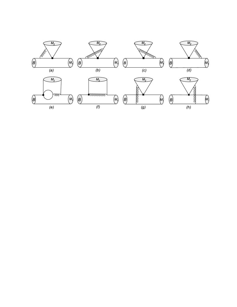
Figure 1: The next to leading order nonfactorizable contributions to the coefficients $a^{p}_{i}$.

Following Beneke and Neubert [13], coefficients $a_{i}^{p}$ can be split into two parts: $a_{i}^{p}=a_{i,I}^{p}+a_{i,II}^{p}$. The first part contains the NF contribution and the sum of nonfactorizable vertex and penguin corrections, while the second one arises from the hard spectator scattering. The coefficients read [13]

$$a_{1,I}=C_{1}+\frac{C_{2}}{N_{C}}\left[1+\frac{C_{F}\alpha_{s}}{4\pi}V_{M_{2}}\right],\qquad\qquad\qquad\qquad a_{1,II}=\frac{C_{2}}{N_{C}}\frac{C_{F}\alpha_{s}}{4\pi}H_{M_{2}M_{1}},$$

$$a_{2,I}=C_{2}+\frac{C_{1}}{N_{C}}\left[1+\frac{C_{F}\alpha_{s}}{4\pi}V_{M_{2}}\right],\qquad\qquad\qquad\qquad a_{2,II}=\frac{C_{1}}{N_{C}}\frac{C_{F}\alpha_{s}}{4\pi}H_{M_{2}M_{1}},$$

$$a_{3,I}=C_{3}+\frac{C_{4}}{N_{C}}\left[1+\frac{C_{F}\alpha_{s}}{4\pi}V_{M_{2}}\right],\qquad\qquad\qquad\qquad a_{3,II}=\frac{C_{4}}{N_{C}}\frac{C_{F}\alpha_{s}}{4\pi}H_{M_{2}M_{1}},$$

$$a_{4,I}^{p}=C_{4}+\frac{C_{3}}{N_{C}}\left[1+\frac{C_{F}\alpha_{s}}{4\pi}V_{M_{2}}\right]+\frac{C_{F}\alpha_{s}}{4\pi}\frac{P^{p}_{M_{2},2}}{N_{C}},\qquad~{}a_{4,II}=\frac{C_{3}}{N_{C}}\frac{C_{F}\alpha_{s}}{4\pi}H_{M_{2}M_{1}},$$

$$a_{5,I}=C_{5}+\frac{C_{6}}{N_{C}}\left[1+\frac{C_{F}\alpha_{s}}{4\pi}(-12-V_{M_{2}})\right],\qquad\qquad a_{5,II}=\frac{C_{6}}{N_{C}}\frac{C_{F}\alpha_{s}}{4\pi}(-H_{M_{2}M_{1}}),$$

$$a_{6,I}^{p}=C_{6}+\frac{C_{5}}{N_{C}}\left[1-6\cdot\frac{C_{F}\alpha_{s}}{4\pi}\right]+\frac{C_{F}\alpha_{s}}{4\pi}\frac{P^{p}_{M_{2},3}}{N_{C}},\qquad~{}a_{6,II}=0,$$

$$a_{7,I}=C_{7}+\frac{C_{8}}{N_{C}}\left[1+\frac{C_{F}\alpha_{s}}{4\pi}(-12-V_{M_{2}})\right],\qquad\qquad~{}a_{7,II}=\frac{C_{8}}{N_{C}}\frac{C_{F}\alpha_{s}}{4\pi}(-H_{M_{2}M_{1}}),$$

$$a_{8,I}^{p}=C_{8}+\frac{C_{7}}{N_{C}}\left[1-6\cdot\frac{C_{F}\alpha_{s}}{4\pi}\right]+\frac{\alpha_{e}}{9\pi}\frac{P^{p,EW}_{M_{2},3}}{N_{C}},\qquad~{}~{}~{}a_{8,II}=0,$$

$$a_{9,I}=C_{9}+\frac{C_{10}}{N_{C}}\left[1+\frac{C_{F}\alpha_{s}}{4\pi}V_{M_{2}}\right],\qquad\qquad\qquad\qquad a_{9,II}=\frac{C_{10}}{N_{C}}\frac{C_{F}\alpha_{s}}{4\pi}H_{M_{2}M_{1}},$$

$$a_{10,I}^{p}=C_{10}+\frac{C_{9}}{N_{C}}\left[1+\frac{C_{F}\alpha_{s}}{4\pi}V_{M_{2}}\right]+\frac{\alpha_{e}}{9\pi}\frac{P^{p,EW}_{M_{2},2}}{N_{C}},\qquad a_{10,II}=\frac{C_{9}}{N_{C}}\frac{C_{F}\alpha_{s}}{4\pi}H_{M_{2}M_{1}},$$ (4)

where $\alpha_{s}\equiv\alpha_{s}(\mu)$, $C_{F}=(N_{C}^{2}-1)/(2N_{C})$, and $N_{C}=3$ is the number of colors. The quantities $V_{M},H_{M_{2}M_{1}},P^{p}_{M,2},P^{p}_{M,3},P^{p,EW}_{M,2}$ and $P^{p,EW}_{M,3}$ consist of convolutions of hard-scattering kernels with meson distribution amplitudes. Specifically, the terms $V_{M}$ come from the vertex corrections in Fig. 1(a)-1(d), $P^{p}_{M,2}$ and $P^{p}_{M,3}~{}(P^{p,EW}_{M,2}$ and $P^{p,EW}_{M,3})$ arise from QCD (EW) penguin contractions and the contributions from the dipole operators as depicted by Fig. 1(e) and 1(f). $H_{M_{2}M_{1}}$ is due to the hard spectator scattering as Fig. 1(g) and 1(h). For the penguin terms, the subscript 2 and 3 indicate the twist 2 and 3 distribution amplitudes of light mesons, respectively.

In Eq.(4), $V_{M}$ $(M=\pi,K)$ contains the nonfactorizable vertex corrections , which is

$$V_{M}=12\ln\frac{m_{b}}{\mu}-18+3\int_{0}^{1}{\rm d}u\left(\frac{1-2u}{1-u}\ln u-i\pi\right)\Phi_{M}(u).$$ (5)

Next, the penguin contributions at the twist-2 are described by the functions

$$P^{p}_{M,2} = C_{1}\left[\frac{2}{3}+\frac{4}{3}\ln\frac{m_{b}}{\mu}-G_{M}(s_{p})\right]+C_{3}\left[\frac{4}{3}+\frac{8}{3}\ln\frac{m_{b}}{\mu}-G_{M}(0)-G_{M}(1)\right]$$

$$+~{}(C_{4}+C_{6})\left[\frac{4n_{f}}{3}\ln\frac{m_{b}}{\mu}-(n_{f}-2)G_{M}(0)-G_{M}(s_{c})-G_{M}(1)\right]$$

$$-~{}C^{eff}_{8g}\int_{0}^{1}{\rm d}u~{}\frac{2\Phi_{M}(u)}{1-u},$$

$$P^{p,EW}_{M,2} = (C_{1}+N_{C}C_{2})\left[\frac{2}{3}+\frac{4}{3}\ln\frac{m_{b}}{\mu}-G_{M}(s_{p})\right]-~{}C^{eff}_{7\gamma}\int_{0}^{1}{\rm d}u~{}\frac{3\Phi_{M}(u)}{1-u},$$ (6)

where $n_{f}=5$ is the number of quark flavors, and $s_{u}=0,s_{c}=(m_{c}/m_{b})^{2}$ are mass ratios involved in the evaluation of the penguin diagrams. The function $G_{M}(s)$ is defined as

$$G_{M}(s) = -4\int_{0}^{1}{\rm d}u\int_{0}^{1}{\rm d}x~{}x\bar{x}\ln{(s-x\bar{x}\bar{u}-i\epsilon)}\Phi_{M}(u).$$ (7)

The twist-3 terms from the penguin diagrams are given by

$$P^{p}_{M,3} = C_{1}\left[\frac{2}{3}+\frac{4}{3}\ln\frac{m_{b}}{\mu}-\widehat{G}_{M}(s_{p})\right]+C_{3}\left[\frac{4}{3}+\frac{8}{3}\ln\frac{m_{b}}{\mu}-\widehat{G}_{M}(0)-\widehat{G}_{M}(1)\right]$$

$$+~{}(C_{4}+C_{6})\left[\frac{4n_{f}}{3}\ln\frac{m_{b}}{\mu}-(n_{f}-2)\widehat{G}_{M}(0)-\widehat{G}_{M}(s_{c})-\widehat{G}_{M}(1)\right]-~{}2C^{eff}_{8g},$$

$$P^{p,EW}_{M,3} = (C_{1}+N_{C}C_{2})\left[\frac{2}{3}+\frac{4}{3}\ln\frac{m_{b}}{\mu}-\widehat{G}_{M}(s_{p})\right]-~{}3C^{eff}_{7\gamma},$$ (8)

with

$$\widehat{G}_{M}(s) = -4\int_{0}^{1}{\rm d}u\int_{0}^{1}{\rm d}x~{}x\bar{x}\ln{(s-x\bar{x}\bar{u}-i\epsilon)}\Phi^{M}_{p}(u).$$ (9)

Finally, the hard spectator interactions can be written as

$$H_{M_{2}M_{1}}=\frac{4\pi^{2}}{N_{C}}\frac{f_{B}f_{M_{1}}}{m_{B}^{2}f_{0}^{B\to M_{1}}(0)}\int^{1}_{0}\frac{{\rm d}\xi}{\xi}\Phi_{B}(\xi)\int^{1}_{0}\frac{{\rm d}u}{\bar{u}}\Phi_{M_{2}}(u)\int^{1}_{0}\frac{{\rm d}v}{\bar{v}}\left[\Phi_{M_{1}}(v)+\frac{2\mu_{M_{1}}}{M_{B}}\Phi^{M_{1}}_{p}(v)\right].$$ (10)

Considering the off-shellness of the gluon in hard scattering kernel, it is natural to associate a scale $\mu_{h}\sim\sqrt{\Lambda_{QCD}m_{b}}$ , rather than $\mu\sim m_{b}$. For the logarithmically divergent integral, we will parameterize it as in [13]: $X_{H}=\int^{1}_{0}{\rm d}u/u=-ln(\Lambda_{QCD}/m_{b})+\varrho_{H}e^{i\phi_{H}}$ $m_{b}/\Lambda_{QCD}$ with $(\varrho_{H},\phi_{H})$ related to the contributions from hard spectator scattering. In the later numerical analysis, we shall take $\Lambda_{QCD}=0.5GeV$, $(\varrho_{h},\phi_{H})=(0,0)$ as our default values.

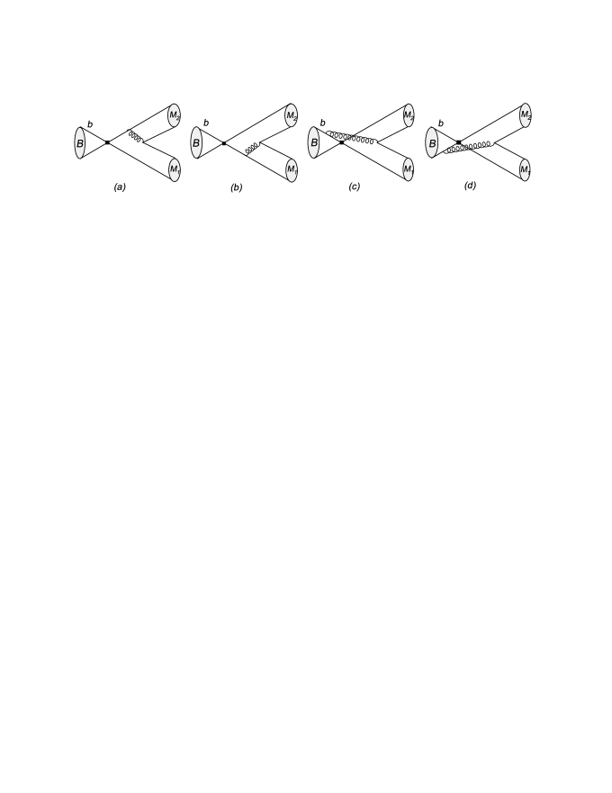
Figure 2: The weak annihilation contributions to the coefficients $b^{p}_{i}$.

At leading order in $\alpha_{s}$, the annihilation contribution can be calculated from the diagrams in Fig.2. The annihilation coefficients $(b_{1},b_{2}),(b_{3},b_{4})$ and $(b^{EW}_{3},b^{EW}_{4})$ correspond to the contributions of the tree, QCD penguins and EW penguins operators insertions, respectively. Using the asymptotic light cone distribution amplitudes of the mesons, and assuming SU(3) flavor symmetry, they can be expressed as

$$b_{1}=\frac{C_{F}}{N_{C}^{2}}C_{1}A^{i}_{1},\hskip 56.9055ptb_{3}=\frac{C_{F}}{N_{C}^{2}}\left[C_{3}A^{i}_{1}+C_{5}\left(A^{i}_{3}+A^{f}_{3}\right)+N_{C}C_{6}A^{f}_{3}\right],$$

$$b_{2}=\frac{C_{F}}{N_{C}^{2}}C_{2}A^{i}_{1},\hskip 56.9055ptb_{4}=\frac{C_{F}}{N_{C}^{2}}\left[C_{4}A^{i}_{1}+C_{6}A^{i}_{2}\right],$$

$$b_{3}^{EW}=\frac{C_{F}}{N_{C}^{2}}\left[C_{9}A^{i}_{1}+C_{7}\left(A^{i}_{3}+A^{f}_{3}\right)+N_{C}C_{8}A^{f}_{3}\right],$$

$$b_{4}^{EW}=\frac{C_{F}}{N_{C}^{2}}\left[C_{10}A^{i}_{1}+C_{8}A^{i}_{2}\right],$$ (11)

and

$$A^{i}_{1}\approx\pi\alpha_{s}\left[18\left(X_{A}-4+\frac{\pi^{2}}{3}\right)+2r^{2}_{\chi}X^{2}_{A}\right],\qquad~{}A^{i}_{2}=A^{i}_{1},\qquad A^{i}_{3}=0,$$

$$A^{f}_{3}\approx 12\pi\alpha_{s}r_{\chi}\left(2X^{2}_{A}-X_{A}\right),\qquad\qquad\qquad\qquad A^{f}_{1}=0,\qquad~{}~{}A^{f}_{2}=0.$$ (12)

Here the superscripts i and f refer to gluon emission from the initial and final state quarks, respectively. The subscript $k$ of $A^{i,f}_{k}$ refers to one of the three possible Dirac structures $\Gamma_{1}\otimes\Gamma_{2}$, namely $k=1$ for $(V-A)\otimes(V-A)$, $k=2$ for $(V-A)\otimes(V+A)$, and $k=3$ for $(-2)(S-P)\otimes(S+P)$. $X_{A}=\int^{1}_{0}{\rm d}u/u$ is a logarithmically divergent integral, and will be phenomenologically parameterized in the calculation as $X_{H}$. As for the hard spectator terms, we will evaluate the various quantities in Eq.(12) at the scale $\mu_{h}=\sqrt{\Lambda_{QCD}m_{b}}$.

With the coefficients in Eq.(4) and (11), we can obtain the decay amplitudes of the SM part $\mathcal{A}^{SM}_{f}$ (the subscript “$f$” denotes the part of QCDF contribution) and $\mathcal{A}^{SM}_{a}$ (the subscript “$a$” denotes the annihilation part). $B\to\pi\pi$ and $\pi K$ decay amplitudes are given in Appendix A.

2.2 R-parity violating SUSY effects in the decays

In the most general superpotential of the minimal supersymmetric Standard Model (MSSM), the RPV superpotential is given by [40]

$$\mathcal{W}_{\not\!R\,} = \mu_{i}\hat{L}_{i}\hat{H}_{u}+\frac{1}{2}\lambda_{[ij]k}\hat{L}_{i}\hat{L}_{j}\hat{E}^{c}_{k}+\lambda^{\prime}_{ijk}\hat{L}_{i}\hat{Q}_{j}\hat{D}^{c}_{k}+\frac{1}{2}\lambda^{\prime\prime}_{i[jk]}\hat{U}^{c}_{i}\hat{D}^{c}_{j}\hat{D}^{c}_{k},$$ (13)

where $\hat{L}$ and $\hat{Q}$ are the SU(2)-doublet lepton and quark superfields and $\hat{E}^{c}$, $\hat{U}^{c}$ and $\hat{D}^{c}$ are the singlet superfields, while i, j and k are generation indices and $c$ denotes a charge conjugate field.

The bilinear RPV superpotential terms $\mu_{i}\hat{L}_{i}\hat{H}_{u}$ can be rotated away by suitable redefining the lepton and Higgs superfields [41]. However, the rotation will generate a soft SUSY breaking bilinear term which would affect our calculation through penguin level. However, the processes discussed in this paper could be induced by tree-level RPV couplings, so that we would neglect sub-leading RPV penguin contributions in this study.

The $\lambda$ and $\lambda^{\prime}$ couplings in Eq.(13) break the lepton number, while the $\lambda^{\prime\prime}$ couplings break the baryon number. There are 27 $\lambda^{\prime}_{ijk}$ couplings, 9 $\lambda_{ijk}$ and 9 $\lambda^{\prime\prime}_{ijk}$ couplings. $\lambda_{[ij]k}$ are antisymmetric with respect to their first two indices, and $\lambda^{\prime\prime}_{i[jk]}$ are antisymmetric with j and k. The antisymmetry of the baryon number violating couplings $\lambda^{\prime\prime}_{i[jk]}$ in the last two indices implies that there are no $\lambda^{\prime\prime}_{ijk}$ operator generating the $\bar{b}\rightarrow\bar{s}s\bar{s}$ and $\bar{b}\rightarrow\bar{d}d\bar{d}$ transitions.

Figure 3: Sleptons exchanging diagrams for nonleptonic B decays.

Figure 4: Squarks exchanging diagrams for nonleptonic B decays.

From Eq.(13), we can obtain the following four fermion effective Hamiltonian due to the sleptons exchange as shown in Fig.3

$$\mathcal{H}^{\prime\not\!R\,}_{2u-2d} = \sum_{i}\frac{\lambda^{\prime}_{ijm}\lambda^{\prime*}_{ikl}}{2m^{2}_{\tilde{e}_{Li}}}\eta^{-8/\beta_{0}}(\bar{d}_{m}\gamma^{\mu}P_{R}d_{l})_{8}(\bar{u}_{k}\gamma_{\mu}P_{L}u_{j})_{8},$$

$$\mathcal{H}^{\prime\not\!R\,}_{4d} = \sum_{i}\frac{\lambda^{\prime}_{ijm}\lambda^{\prime*}_{ikl}}{2m^{2}_{\tilde{\nu}_{Li}}}\eta^{-8/\beta_{0}}(\bar{d}_{m}\gamma^{\mu}P_{R}d_{l})_{8}(\bar{d}_{k}\gamma_{\mu}P_{L}d_{j})_{8}.$$ (14)

The four fermion effective Hamiltonian due to the squarks exchanging as shown in Fig. 4 are

$$\mathcal{H}^{\prime\prime\not\!R\,}_{2u-2d} = \sum_{n}\frac{\lambda^{\prime\prime}_{ikn}\lambda^{\prime\prime*}_{jln}}{2m^{2}_{\tilde{d}_{n}}}\eta^{-4/\beta_{0}}\left\{\left[(\bar{u}_{i}\gamma^{\mu}P_{R}u_{j})_{1}(\bar{d}_{k}\gamma_{\mu}P_{R}d_{l})_{1}-(\bar{u}_{i}\gamma^{\mu}P_{R}u_{j})_{8}(\bar{d}_{k}\gamma_{\mu}P_{R}d_{l})_{8}\right]\right.$$

$$\hskip 85.35826pt-\left[\left.(\bar{d}_{k}\gamma^{\mu}P_{R}u_{j})_{1}(\bar{u}_{i}\gamma_{\mu}P_{R}d_{l})_{1}-(\bar{d}_{k}\gamma^{\mu}P_{R}u_{j})_{8}(\bar{u}_{i}\gamma_{\mu}P_{R}d_{l})_{8}\right]\right\},$$

$$\mathcal{H}^{\prime\prime\not\!R\,}_{4d} = \sum_{n}\frac{\lambda^{\prime\prime}_{nik}\lambda^{\prime\prime*}_{njl}}{4m^{2}_{\tilde{u}_{n}}}\eta^{-4/\beta_{0}}\left[(\bar{d}_{i}\gamma^{\mu}P_{R}d_{j})_{1}(\bar{d}_{k}\gamma_{\mu}P_{R}d_{l})_{1}-(\bar{d}_{i}\gamma^{\mu}P_{R}d_{j})_{8}(\bar{d}_{k}\gamma_{\mu}P_{R}d_{l})_{8}\right].$$ (15)

where $P_{L}=\frac{1-\gamma_{5}}{2},P_{R}=\frac{1+\gamma_{5}}{2},\eta=\frac{\alpha_{s}(m_{\hat{f}_{i}})}{\alpha_{s}(m_{b})}$ and $\beta_{0}=11-\frac{2}{3}n_{f}$. The subscript for the currents $(j_{\mu})_{1,8}$ represents the current in the color singlet and octet, respectively. The coefficients $\eta^{-4/\beta_{0}}$ and $\eta^{-8/\beta_{0}}$ are due to the running from the sfermion mass scale $m_{\hat{f}_{i}}$ (100 GeV assumed) down to the $m_{b}$ scale. Since it is always assumed in phenomenology for numerical display that only one sfermion contributes at one time, we neglect the mixing between the operators when we use the renormalization group equation (RGE) to run $\mathcal{H}^{\not\!R\,}$ down to the low scale.

Generally, the RPV couplings can be complex and their phases may induce new contributions to the $CP$ violation, so we write them as

$$\lambda_{ijk}\lambda^{*}_{lmn}=|\lambda_{ijk}\lambda^{*}_{lmn}|~{}e^{i\phi_{\not\!R\,}},~{}~{}~{}~{}~{}\lambda^{*}_{ijk}\lambda_{lmn}=|\lambda_{ijk}\lambda^{*}_{lmn}|~{}e^{-i\phi_{\not\!R\,}},$$ (16)

here $\phi_{\not\!R\,}$ is the RPV weak phase, which could be any value between 0 and $\pi$. To include the effect of $\pi\leq\phi_{\not\!R\,}\leq 2\pi$, $|\lambda_{ijk}\lambda^{*}_{lmn}|$ is allowed to take both positive and negative values for simplicity.

Compared with the operators in the $\mathcal{H}^{SM}_{eff}$, there are new operators $(\bar{q}_{2}q_{3})_{V\pm A}(\bar{b}q_{1})_{V+A}$ in the $\mathcal{H}^{\not\!R\,}$. For $B\to PP$ decays, since

$$\langle P|~{}\bar{q}_{1}\gamma_{\mu}(1-\gamma_{5})q_{2}|~{}0\rangle=-\langle P|~{}\bar{q}_{1}\gamma_{\mu}(1+\gamma_{5})q_{2}|~{}0\rangle=-\langle P|~{}\bar{q}_{1}\gamma_{\mu}\gamma_{5}q_{2}|~{}0\rangle,$$ (17)

$$\langle P|~{}\bar{q}\gamma_{\mu}(1-\gamma_{5})b~{}|~{}B\rangle=\langle P|~{}\bar{q}\gamma_{\mu}(1+\gamma_{5})b~{}|~{}B\rangle=\langle P|~{}\bar{q}\gamma_{\mu}b~{}|~{}B\rangle,\hskip 28.45274pt$$ (18)

the RPV contribution to the decay amplitude will modify the SM amplitude by an overall relation.

Since we are considering the leading effects of RPV, we need only evaluate the nonfactorizable vertex corrections and hard spectator scattering contributions. We ignore the RPV penguin contributions, which are expected to be small even compared to the SM penguin amplitudes, due to the smallness of the relevant RPV couplings compared with the SM gauge couplings. As shown in Ref. [34], the bounds on the RPV couplings are insensitive to the inclusion of RPV penguins. We also have neglected the annihilation contributions in the RPV amplitudes. The R-parity violating part of the decay amplitudes $\mathcal{A}^{\not\!R\,}$ can be found in Appendix B.

2.3 The branching ratio and the direct $CP$ asymmetries

With the QCDF approach, we can get the total decay amplitude

$$\mathcal{A}(B\rightarrow P_{1}P_{2})=\mathcal{A}^{SM}_{f}(B\rightarrow P_{1}P_{2})+\mathcal{A}^{SM}_{a}(B\rightarrow P_{1}P_{2})+\mathcal{A}^{\not\!R\,}(B\rightarrow P_{1}P_{2}).$$ (19)

The expressions for the SM amplitude $\mathcal{A}^{SM}_{f,a}$ and the RPV amplitude $\mathcal{A}^{\not\!R\,}$ are presented in Appendices A and B, respectively. From the amplitude in Eq. (19), the branching ratio reads

$$\mathcal{B}r(B\rightarrow P_{1}P_{2})=\frac{\tau_{B}|p_{c}|}{8\pi m_{B}^{2}}\left|\mathcal{A}(B\rightarrow P_{1}P_{2})\right|^{2}S,$$ (20)

where $S=1/2$ for identical $P_{1}$ and $P_{2}$, $S=1$ otherwise, $\tau_{B}$ is the B lifetime, $|p_{c}|$ is the center of mass momentum of light mesons in the rest frame of B meson, and given by

$$|p_{c}|=\frac{1}{2m_{B}}\sqrt{[m_{B}^{2}-(m_{P_{1}}+m_{P_{2}})^{2}][m_{B}^{2}-(m_{P_{1}}-m_{P_{2}})^{2}]}.$$ (21)

The $CP$ averaged branching ratios are defined by

$$\mathcal{B}r(B^{\pm}\to P_{1}^{\pm}P_{2}) \equiv \frac{1}{2}\left[\mathcal{B}r(B^{-}\to P_{1}^{-}\bar{P}^{0}_{2})+\mathcal{B}r(B^{+}\to P_{1}^{+}P^{0}_{2})\right],$$

$$\mathcal{B}r(B_{d}\to P_{1}^{\pm}P_{2}^{\mp}) \equiv \frac{1}{2}\left[\mathcal{B}r(\bar{B}^{0}_{d}\to P_{1}^{+}P_{2}^{-})+\mathcal{B}r(B^{0}_{d}\to P_{1}^{-}P_{2}^{+})\right],$$ (22)

$$\mathcal{B}r(B_{d}\to P_{1}^{0}~{}P_{2}^{0}) \equiv \frac{1}{2}\left[\mathcal{B}r(\bar{B}^{0}_{d}\to P_{1}^{0}\bar{P}_{2}^{0})+\mathcal{B}r(B^{0}_{d}\to P_{1}^{0}P_{2}^{0})\right].$$

The direct $CP$ asymmetry is defined by

$$\mathcal{A}_{CP}^{dir}=\frac{\mathcal{B}r(\bar{B}\to\bar{f})-\mathcal{B}r(B\to f)}{\mathcal{B}r(\bar{B}\to\bar{f})+\mathcal{B}r(B\to f)}.$$ (23)

3 Input parameters

A. Wilson coefficients
For numerical analyzes, we use the next-to-leading Wilson coefficients calculated in the naive dimensional regularization (NDR) scheme and at $m_{b}$ scale [35]

$$C_{1}=1.082,~{}~{}~{}C_{2}=-0.185,~{}~{}~{}C_{3}=0.014,~{}~{}~{}C_{4}=-0.035,~{}~{}~{}C_{5}=0.009,$$

$$C_{6}=-0.041,~{}~{}~{}C_{7}/\alpha_{e}=-0.002,~{}~{}~{}C_{8}/\alpha_{e}=0.054,~{}~{}~{}C_{9}/\alpha_{e}=-1.292,$$

$$C_{10}/\alpha_{e}=0.263,~{}~{}~{}C^{eff}_{7\gamma}=-0.299,~{}~{}~{}C^{eff}_{8g}=-0.143.$$

B. The CKM matrix element
The magnitude of the CKM elements are taken from [42]

$$\begin{array}[]{lll}|V_{ud}|=0.9738\pm 0.0005,&|V_{us}|=0.2200\pm 0.0026,&|V_{ub}|=0.00367\pm 0.00047,\\ |V_{cd}|=-0.224\pm 0.012,&|V_{cs}|=0.996\pm 0.013,&|V_{cb}|=0.0413\pm 0.0015,\\ |V_{tb}^{*}V_{td}|=0.0083\pm 0.0016&|V_{tb}V_{ts}^{*}|=-0.047\pm 0.008,&\\ \end{array}$$ (24)

and the weak phases $\gamma=60^{\circ}\pm 14^{\circ}$, sin$(2\beta)=0.736\pm 0.049$.
C. Masses and lifetime
There are two types of quark mass in our analysis. One type is the pole mass which appears in the loop integration. Here we fix them as

$$m_{u}=m_{d}=m_{s}=0,~{}~{}~{}~{}m_{c}=1.47~{}\mbox{GeV},~{}~{}~{}~{}m_{b}=4.8~{}\mbox{GeV}.$$

The other type quark mass appears in the hadronic matrix elements and the chirally enhanced factor $r_{\chi}^{P}=\frac{2\mu_{p}}{\overline{m}_{b}}$ through the equations of motion, which are renormalization scale dependent. We shall use the 2004 Particle Data Group values [42] for discussion (the central values are taken as our default values)

$$\overline{m}_{u}(2{\rm GeV})=0.0015\sim 0.004~{}{\rm GeV},~{}~{}~{}~{}\overline{m}_{d}(2{\rm GeV})=0.004\sim 0.008~{}{\rm GeV},$$

$$\overline{m}_{s}(2{\rm GeV})=0.08\sim 0.13~{}{\rm GeV},~{}~{}~{}~{}~{}~{}~{}~{}~{}\overline{m}_{b}(\overline{m}_{b})=4.1\sim 4.4~{}{\rm GeV},$$

and then employ the formula in Ref. [35]

$$\overline{m}(\mu)=\overline{m}(\mu_{0})\left[\frac{\alpha_{s}(\mu)}{\alpha_{s}(\mu_{0})}\right]^{\frac{\gamma^{(0)}_{m}}{2\beta_{0}}}\left[1+\left(\frac{\gamma^{(1)}_{m}}{2\beta_{0}}-\frac{\beta_{1}\gamma^{(0)}_{m}}{2\beta_{0}^{2}}\right)\frac{\alpha_{s}(\mu)-\alpha_{s}(\mu_{0})}{4\pi}\right]$$

to obtain the current quark masses at $\mu$ scale. The definitions of $\gamma^{(0)}_{m},\gamma^{(1)}_{m},\beta_{0},\beta_{1}$ can be found in [35].
D. The light cone distribution amplitudes (LCDAs) of the pseudoscalar meson
For the LCDAs of the pseudoscalar meson, we use the asymptotic form [43, 44]

$$\Phi_{P}(x)=6x(1-x),~{}~{}~{}~{}~{}~{}~{}~{}~{}~{}~{}\Phi^{P}_{p}(x)=1.$$ (25)

We adopt the moments of the $\Phi_{1}^{B}(\xi)$ defined in Ref. [13, 33] for our numerical evaluation

$$\int_{0}^{1}{\rm d}\xi\frac{\Phi_{1}^{B}(\xi)}{\xi}=\frac{m_{B}}{\lambda_{B}},$$ (26)

with $\lambda_{B}=0.46$ GeV [45]. The quantity $\lambda_{B}$ parameterizes our ignorance about the $B$ meson distribution amplitudes and thus brings considerable theoretical uncertainty.
E. The decay constants and form factors
For the decay constants, we take the latest light-cone QCD sum rule (LCSR) results [46] in our calculations

$f_{B}=0.162$ GeV,

$f_{K}=0.16$ GeV,

$f_{\pi}=0.131$ GeV.

For the form factors involving $B\to K$ and $B\to\pi$ transitions, we adopt the center values of the results [46]

$$f^{B\to K}_{0}(0)=0.331,~{}~{}~{}~{}~{}~{}~{}~{}~{}~{}~{}~{}~{}~{}f^{B\to\pi}_{0}(0)=0.258.$$

4 Numerical results and analysis

We will present our numerical results in this section. At first, we will show our estimations in the SM by taking the center value of the input parameters and compare with the relevant experimental data. Then, we will consider the RPV effects and constrain the relevant RPV couplings by the averages of Belle and BABAR measurements of the $CP$ averaged branching ratios and the direct CP asymmetries.

When considering the RPV effects, we will use the input parameters and the experimental data which are varied randomly within $1\sigma$ level and $2\sigma$ level, respectively. In the SM, the weak phase $\gamma$ is well constrained, however, with the presence of RPV, this constraint may be relaxed. We would not take $\gamma$ within the SM range, but vary it randomly in the range of 0 to $\pi$ to obtain conservative limits on RPV couplings. We assume that only one sfermion contributes at one time with a mass of 100 GeV. So for other values of the sfermion masses, the bounds on the couplings in this paper can be easily obtained by scaling them by factor $\tilde{f}^{2}\equiv(\frac{m_{\tilde{f}}}{100GeV})^{2}$.

The main numerical results in the SM and the relevant data from the Belle collaborations [7, 8, 9, 10, 11, 12] and BABAR collaborations[1, 2, 3, 4, 5, 6] are presented in Table I, II and III, which show the results for the $CP$ averaged branching ratios, the direct $CP$ asymmetries and the ratios of the $CP$ averaged branching ratios, respectively.

Table I: The $CP$ averaged branching ratios of $B\to\pi\pi,\pi K$ in the SM(in unit of $10^{-6}$). Experimental data from BABAR and Belle and the SM predictions in the framework of NF and QCDF, where $\mathcal{B}r^{f}$ and $\mathcal{B}r^{f+a}$ denote the results without and with the contributions from weak annihilation, respectively.

QCDF
Decays	Belle	BABAR	Average	NF	$\mathcal{B}r^{f}$	$\mathcal{B}r^{f+a}$
$B_{d}\rightarrow\pi^{\pm}\pi^{\mp}$	$4.4\pm 0.6\pm 0.3$	$4.7\pm 0.6\pm 0.2$	$4.56\pm 0.46$	7.56	7.88	8.33
$B^{\pm}\rightarrow\pi^{0}\pi^{\pm}$	$5.0\pm 1.2\pm 0.5$	$5.8\pm 0.6\pm 0.4$	$5.61\pm 0.63$	5.19	4.90	4.90
$B_{d}\rightarrow\pi^{0}\pi^{0}$	$2.3^{+0.4+0.2}_{-0.5-0.3}$	$1.17\pm 0.32\pm 0.10$	$1.45\pm 0.29$	0.17	0.16	0.18
$B^{\pm}\rightarrow\pi^{\pm}K$	$22.0\pm 1.9\pm 1.1$	$26.0\pm 1.3\pm 1.0$	$24.57\pm 1.31$	12.42	14.77	17.09
$B^{\pm}\rightarrow\pi^{0}K^{\pm}$	$12.0\pm 1.3^{+1.3}_{-0.9}$	$12.0\pm 0.7\pm 0.6$	$12.00\pm 0.81$	7.23	8.36	9.57
$B_{d}\rightarrow\pi^{\pm}K^{\mp}$	$18.5\pm 1.0\pm 0.9$	$17.9\pm 0.9\pm 0.7$	$18.15\pm 0.87$	9.93	11.64	13.54
$B_{d}\rightarrow\pi^{0}K$	$11.7\pm 2.3^{+1.2}_{-1.3}$	$11.4\pm 0.9\pm 0.6$	$11.44\pm 1.00$	4.20	5.06	5.97

Table II: The direct $CP$ asymmetries $\mathcal{A}^{dir}_{CP}$ (in unit of $10^{-2}$) for $B\to\pi\pi,\pi K$. Experimental data from BABAR and Belle. $\mathcal{A}^{f}_{CP}$ and $\mathcal{A}^{f+a}_{CP}$ are defined in the similar way as branching ratios in Table I.

QCDF
Decays	Belle	BABAR	Average	$\mathcal{A}^{f}_{CP}$	$\mathcal{A}^{f+a}_{CP}$
$B_{d}\rightarrow\pi^{\pm}\pi^{\mp}$	$58\pm 15\pm 7$	$9\pm 15\pm 4$	$31.93\pm 11.32$	-5.86	-5.68
$B^{\pm}\rightarrow\pi^{0}\pi^{\pm}$	$2\pm 8\pm 1$	$-1\pm 10\pm 2$	$0.85\pm 6.32$	-0.07	-0.07
$B_{d}\rightarrow\pi^{0}\pi^{0}$	$44^{+53}_{-52}\pm 17$	$12\pm 56\pm 6$	$28.33\pm 39.42$	63.04	60.55
$B^{\pm}\rightarrow\pi^{\pm}K$	$5\pm 5\pm 1$	$-9\pm 5\pm 1$	$-2.00\pm 3.61$	1.23	1.13
$B^{\pm}\rightarrow\pi^{0}K^{\pm}$	$4\pm 4\pm 2$	$6\pm 6\pm 1$	$4.70\pm 3.60$	8.12	7.29
$B_{d}\rightarrow\pi^{\pm}K^{\mp}$	$-11.3\pm 2.2\pm 8$	$-13.3\pm 3\pm 0.9$	$-12.02\pm 1.86$	6.32	5.50
$B_{d}\rightarrow\pi^{0}K$	$-12\pm 20\pm 9$	$-6\pm 18\pm 6$	$-8.57\pm 14.35$	-2.45	-2.19

Table III: The ratios of the $CP$ averaged branching ratios.

QCDF
Ratios	Exp.	NF	without ann.	with ann.
$R^{\pi\pi}_{+-}$	$2.30\pm 0.35$	$1.28$	$1.16$	1.10
$R^{\pi\pi}_{00}$	$0.66\pm 0.14$	$0.04$	$0.04$	0.04
$R$	$0.79\pm 0.06$	$0.80$	$0.79$	0.79
$R_{c}$	$0.98\pm 0.08$	$1.16$	$1.13$	1.12
$R_{n}$	$0.79\pm 0.08$	$1.18$	$1.15$	1.13

From Table I, II, III, we can see the puzzle in $B\to\pi\pi,\pi K$ which we have already mentioned in the introduction. For example, the new experimental data for $B\to\pi^{0}\pi^{0},\pi^{0}K^{0}$ branching ratios are significantly larger than the SM predictions, moreover, the expected relation $A^{dir}_{CP}(B^{0}\to\pi^{\pm}K^{\mp})\approx A^{dir}_{CP}(B^{\pm}\to\pi^{0}K^{\pm})$ obviously contradict to the experimental data, even with the opposite sign for them, the value of $R_{n}$ is significantly lower than $R_{c}$, and so on.

Now we turn to the RPV effects which may give possible solutions to the puzzle. We use the $CP$ averaged branching ratios, the direct $CP$ asymmetries and the relevant experimental averages of Belle and BABAR to constrain the spaces of the RPV parameters. As known, data on low energy processes can be used to impose rather strictly constraints on many of these couplings. The random variation of the parameters subjecting to the constraints as discussed above leads to the scatter plots displayed in Fig. 5 and 6.

Figure 5: The allowed parameter spaces for the relevant RPV couplings constrained by $B\to\pi\pi$.

The $B\to\pi\pi$ decays involve the quark level processes $\bar{b}\to\bar{d}q\bar{q}~{}(q=u,d)$. The all three RPV couplings maybe resolve the $B\to\pi\pi$ puzzle, which has been shown in Fig.5. These allowed parameter spaces are essentially controlled by the $CP$ averaged branching ratios and the direct $CP$ asymmetries of different $\pi\pi$ modes. From Fig. 5, we can see that RPV weak phase is not constrained so much, but the relevant magnitude of the RPV couplings are constrained within rather narrow ranges. We can obtain the allowed parameter spaces for the relevant couplings, which are summarized in Table IV. For comparison, we also list the existing bounds on these quadric coupling products [25, 32].

Table IV: Bounds for the relevant RPV coupling constants by $B\to\pi\pi$ decays for 100 GeV sfermions and previous bounds are listed for comparison.

Couplings	Bounds	Process	Previous bounds
$|\lambda^{\prime\prime}_{132}\lambda^{\prime\prime}_{112}|$	$[5.4\times 10^{-4},~{}2.9\times 10^{-3}]$	$B_{d}\to\pi^{\pm}\pi^{\mp},\pi^{0}\pi^{0}$	$<5.0\times 10^{-3}$ [25]
$|\lambda^{\prime}_{i13}\lambda^{\prime}_{i11}|$	$[2.7\times 10^{-4},~{}7.7\times 10^{-4}]$	$B_{d}\to\pi^{\pm}\pi^{\mp},\pi^{0}\pi^{0}$	$<2.5\times 10^{-3}$ [25]
$|\lambda^{\prime}_{i11}\lambda^{\prime}_{i31}|$	$[3.8\times 10^{-4},~{}1.0\times 10^{-3}]$	$B\to\pi^{0}\pi^{\pm},\pi^{0}\pi^{0}$	$<2.0\times 10^{-3}$ [32]

We note that since the quark content of $\pi^{0}$ is antisymmetric combination $(u\bar{u}-d\bar{d})/\sqrt{2}$, the decays $B\to\pi^{0}\pi^{\pm},\pi^{0}\pi^{0}$ could be induced by superpartners of both up-type and down-type fermions in RPV SUSY. For example, $\bar{b}\rightarrow\bar{d}d\bar{d}$ could be induced by sneutrino, while $\bar{b}\rightarrow\bar{u}u\bar{d}$ could be induced by slepton with the same $\lambda^{\prime}_{i13}\lambda^{\prime*}_{i11}$ product. We take $\frac{\lambda^{\prime}_{i13}\lambda^{\prime*}_{i11}}{m^{2}_{\tilde{e}_{i}}}$ and $\frac{\lambda^{\prime}_{i13}\lambda^{\prime*}_{i11}}{m^{2}_{\tilde{\nu}_{i}}}$ contribute to $\bar{b}\rightarrow\bar{u}u\bar{d}$ and $\bar{b}\rightarrow\bar{d}d\bar{d}$ at the same time, and the effects of $\lambda^{\prime}_{i13}\lambda^{\prime*}_{i11}$ will be summed. So that $\lambda^{\prime}_{i13}\lambda^{\prime*}_{i11}$ in amplitudes of $B^{\pm}\to\pi^{0}\pi^{\pm}$ is cancelled and in amplitudes of $B_{d}\to\pi^{0}\pi^{0}$ is partly cancelled if taking $m_{\tilde{e}_{i}}=m_{\tilde{\nu}_{i}}$.

The $B\to\pi K$ processes are due to $\bar{b}\to\bar{s}q\bar{q}~{}(q=u,d)$ transitions at quark level. There are six RPV coupling constants contributing the four $B\to\pi K$ decay modes. We scan the parameter space for possible solutions, and find that only four pairs of RPV couplings, $\lambda^{\prime\prime}_{i31}\lambda^{\prime\prime}_{i21}$, $\lambda^{\prime\prime}_{131}\lambda^{\prime\prime}_{121}$, $\lambda^{\prime}_{i13}\lambda^{\prime}_{i12}$ and $\lambda^{\prime}_{i21}\lambda^{\prime}_{i31}$, can survive after satisfying all relevant experimental data of $B\to\pi K$ decays. But we do not get the solutions to the experimental data at $2\sigma$ level with the other two pairs of RPV coupling constants, $\lambda^{\prime}_{i23}\lambda^{\prime}_{i11}$ and $\lambda^{\prime}_{i11}\lambda^{\prime}_{i32}$. Figure 6 displays the allowed ranges for RPV couplings which satisfy all relevant experimental data of the $B\to\pi K$ decays. The constraints for the four RPV couplings are summarized in Table V. For comparison, we also list the pervious bounds [25, 32].

Figure 6: The allowed parameter spaces for the relevant RPV couplings bounded by $B\to\pi K$. We have not listed the RPV couplings, $\lambda^{\prime}_{i23}\lambda^{\prime}_{i11}$ and $\lambda^{\prime}_{i11}\lambda^{\prime}_{i32}$, for which we have not found the allowed space.

Table V: Bounds for the relevant RPV coupling couplings for 100 GeV sfermions by $B\to\pi K$ decays and previous bounds are also listed.

Couplings	Bounds	Process	Previous bounds
$|\lambda^{\prime\prime}_{i31}\lambda^{\prime\prime}_{i21}|$	${{}_{[3.7\times 10^{-4},~{}4.6\times 10^{-3}]}^{[13.6\times 10^{-3},~{}15.8\times 10^{-3}]}}$	$B^{\pm}\to\pi^{\pm}K,\pi^{0}K^{\pm}$	$<4.\times 10^{-3}\cite[cite]{[\@@bibref{}{report}{}{}]}$
$|\lambda^{\prime\prime}_{131}\lambda^{\prime\prime}_{121}|$	${{}_{[6.1\times 10^{-4},~{}4.6\times 10^{-3}]}^{[5.6\times 10^{-3},~{}7.2\times 10^{-3}]}}$	$B\to\pi^{0}K^{\pm},\pi^{\pm}K^{\mp},\pi^{0}K$	$<4.\times 10^{-3}\cite[cite]{[\@@bibref{}{report}{}{}]}$
$|\lambda^{\prime}_{i13}\lambda^{\prime}_{i12}|$	$[3.6\times 10^{-4},1.1\times 10^{-3}]$	four modes of $\pi K$	$<5.7\times 10^{-3}\cite[cite]{[\@@bibref{}{report}{}{}]}$
$|\lambda^{\prime}_{i21}\lambda^{\prime}_{i31}|$	${{}_{[6.1\times 10^{-4},~{}8.7\times 10^{-4}]}^{[1.1\times 10^{-3},~{}1.2\times 10^{-3}]}}$	$B\to\pi^{\pm}K,\pi^{0}K^{\pm},\pi^{0}K$	$<1.3\times 10^{-3}\cite[cite]{[\@@bibref{}{hexg}{}{}]}$

For the coupling $\lambda^{\prime\prime}_{i31}\lambda^{\prime\prime}_{i21}$, we get two ranges by the $CP$ averaged branching ratios and the direct $CP$ asymmetries of $B\to\pi K$. The bound for this coupling is $10^{-1}\sim 10^{-2}$ by branching ratios of $B\to\pi K$ in [32], and the limit of $\lambda^{\prime\prime}_{i3k}\lambda^{\prime\prime}_{i2k}$ is 0.16 by $B\to K^{*}\gamma$ decay [25]. So both spaces of $\lambda^{\prime\prime}_{i31}\lambda^{\prime\prime}_{i21}$ may be allowed. The $\lambda^{\prime\prime}_{131}\lambda^{\prime\prime}_{121}$ also have two ranges, we may get only the space $|\lambda^{\prime\prime}_{131}\lambda^{\prime\prime}_{121}|\in[0.61\times 10^{-3},4.60\times 10^{-3}]$ if considering the constraint for $\lambda^{\prime\prime}_{i31}\lambda^{\prime\prime}_{i21}$. The bounds for couplings $\lambda^{\prime}_{i13}\lambda^{\prime}_{i12}$ and $\lambda^{\prime}_{i21}\lambda^{\prime}_{i31}$ are obtained by four or three decay modes of $B\to\pi K$, their ranges are also very narrow. For the RPV couplings $\lambda^{\prime}_{i23}\lambda^{\prime}_{i11}$ and $\lambda^{\prime}_{i11}\lambda^{\prime}_{i32}$, we have not obtained their solutions to the puzzles.

The $B^{\pm}\to\pi^{0}K^{\pm}$ and $B^{0}\to\pi^{0}K^{0}$ decays could be induced by superpartners of both up-type and down-type fermions, $\bar{b}\rightarrow\bar{d}d\bar{s}$ could be induced by sneutrino, while $\bar{b}\rightarrow\bar{u}u\bar{s}$ could be induced by slepton with the same $\lambda^{\prime}_{i13}\lambda^{\prime*}_{i12}$ product. For the same reason as in $B\to\pi^{0}\pi^{\pm},\pi^{0}\pi^{0}$, the effects of $\lambda^{\prime}_{i13}\lambda^{\prime*}_{i12}$ have been summed.

The above analysis has shown that the puzzles in the $B\to\pi\pi,\pi K$ decays can be resolved with RPV effects, however, the solution parameter spaces are always very narrow. The allowed spaces constrained by the $B\to\pi\pi,\pi K$ decays are consistent with that by $B\to VV$ decays in our previous study [31].

5 Conclusions

The recent observations of $B\to\pi\pi,~{}\pi K$ decays which are inconsistent with the SM expectations represent a challenge for theoretical interpreting. We have employed the QCDF to present a study of the RPV effects in the $B\to\pi\pi,\pi K$ decays. Our analysis has shown that a set of RPV couplings play an important role to resolve the discrepancies between the theoretical predictions in the SM and the experimental data. However, the windows of the RPV couplings intervals are found to be always very narrow. It implies that these couplings, part or all of them, might be pinned down from the rich experimental phenomena in these decays. However, it also implies the window could be closed easily with refined measurements from experiments in the near future.

It should be noted that some of the $\lambda^{\prime}$ couplings can generate sizable neutrino masses [41, 47]. Allanach et al. have obtained quite strong upper bound $\lambda^{\prime}_{ijj}<10^{-3}$ in the RPV mSUGRA model. Our bounds for quadric products $|\lambda^{\prime}_{i13}\lambda^{\prime}_{i11}|$ and $|\lambda^{\prime}_{i11}\lambda^{\prime}_{i31}|$ are of order of $10^{-3}-10^{-4}$. So combining their constraints from neutrino masses and ours from $B\to\pi\pi$ decays, the $\lambda^{\prime}$ resolution window might be closed. However, we note that the constraints on $\lambda^{\prime}$ from neutrino masses would depend on the explicit neutrino masses models with trilinear couplings only, bilinear couplings only, or both[41].

Furthermore, the $\lambda^{\prime}_{111}$ coupling has been constrained as low as $|\lambda^{\prime}_{111}|<5.2\times 10^{-4}$ by neutrino-less double beta decay[48]. There are also strong bounds $|\lambda^{\prime\prime}_{121}|<10^{-4}$ and $|\lambda^{\prime\prime}_{131}|<10^{-4}$ from double nucleon decay[49] and neutron oscillations[49, 50], respectively. Combining these strong bounds, our solutions with $\lambda^{\prime}_{113}\lambda^{\prime}_{111}$, $\lambda^{\prime}_{111}\lambda^{\prime}_{131}$ and $\lambda^{\prime\prime}_{131}\lambda^{\prime\prime}_{121}$ RPV products should be excluded. However, from the comprehensive collation of bounds upon trilinear RPV couplings in Ref.[51], our other solutions still remain. Explicitly, the $B\to\pi\pi$ puzzle could be resolved by the presences of RPV couplings $\lambda^{\prime\prime}_{132}\lambda^{\prime\prime}_{112}$, $\lambda^{\prime}_{i11}\lambda^{\prime}_{i31}$ and $\lambda^{\prime}_{i13}\lambda^{\prime}_{i11}$ with $i\neq 1$, while the $B\to\pi K$ puzzle could be resolved by $\lambda^{\prime\prime}_{i31}\lambda^{\prime\prime}_{i21}$ ($i\neq 1$), $\lambda^{\prime}_{i13}\lambda^{\prime}_{i12}$ and $\lambda^{\prime}_{i21}\lambda^{\prime}_{i31}$.

Generally, we can believe that QCDF calculations for the direct $CP$ asymmetries could be much more accurate than that for the branching ratios, since many uncertainties could be cancelled in the ratios. Therefore the constraints from the direct $CP$ asymmetries would be more well-founded than those only from branching ratio measurements [32]. Comparing our prediction with the recent experimental data within $2\sigma$ level about the $CP$ averaged branching ratios and the direct $CP$ asymmetries, we have obtained bounds on the relevant products of RPV couplings. With more data from BABAR and Belle, one can significantly shrink the allowed parameter spaces for RPV couplings. We find that these constraints are consistent with the previous bounds, even most of them are stronger than the existing limits [25, 31, 32], which may be useful for further study of RPV phenomenology.

To summarize, we have shown that the $B\to\pi\pi$ puzzle and the $B\to\pi K$ puzzle could be resolved in the RPV SUSY. Using the latest experimental data, we get the allowed values of the relevant RPV couplings, and the most of these new constraints are stronger than the existing bounds.

Appendix A . The amplitudes in the SM

The factorized matrix elements are defined by

$$A_{M_{1}M_{2}} \equiv \langle M_{2}|(\bar{q}_{1}q_{2})_{(V-A)}|0\rangle\langle M_{1}|(\bar{q}_{3}b)_{(V-A)}|B\rangle=i(m^{2}_{B}-m^{2}_{M_{1}})f_{0}^{B\to M_{1}}(m_{M_{2}}^{2})f_{M_{2}},$$ (27)

$$B_{M_{1}M_{2}} \equiv \langle M_{1}M_{2}|(\bar{q}_{1}q_{2})_{(V-A)}|0\rangle\langle 0|(\bar{q}_{3}b)_{(V-A)}|B\rangle=if_{B}f_{M_{1}}f_{M_{2}}.$$ (28)

$$\mathcal{A}^{SM}_{f}(\bar{B}^{0}\rightarrow\pi^{+}\pi^{-}) = \frac{G_{F}}{\sqrt{2}}\left\{\lambda_{ud}a_{1}+\lambda_{pd}\left[a_{4}^{p}+a_{10}^{p}+r^{\pi}_{\chi}(a_{6}^{p}+a^{p}_{8})\right]\right\}A_{\pi\pi},$$ (29)

$$\mathcal{A}^{SM}_{f}(B^{-}\rightarrow\pi^{-}\pi^{0}) = \frac{G_{F}}{2}\left\{\lambda_{ud}(a_{1}+a_{2})+\frac{3}{2}\lambda_{pd}\left[-a_{7}+a_{9}+a_{10}^{p}+r^{\pi}_{\chi}a^{p}_{8}\right]\right\}A_{\pi\pi},$$ (30)

$$\mathcal{A}^{SM}_{f}(\bar{B}^{0}\rightarrow\pi^{0}\pi^{0}) = -\frac{G_{F}}{\sqrt{2}}\left\{\lambda_{ud}a_{2}+\lambda_{pd}\left[-a_{4}^{p}+\frac{3}{2}(-a_{7}+a_{9})+\frac{1}{2}a^{p}_{10}-r^{\pi}_{\chi}(a^{p}_{6}-\frac{1}{2}a_{8}^{p})\right]\right\}A_{\pi\pi},$$

$$\mathcal{A}^{SM}_{f}(B^{-}\rightarrow\pi^{-}\bar{K}^{0}) = \frac{G_{F}}{\sqrt{2}}\left\{\lambda_{ps}\left[\left(a_{4}^{p}-\frac{1}{2}a_{10}^{p}\right)+r^{K}_{\chi}\left(a_{6}^{p}-\frac{1}{2}a^{p}_{8}\right)\right]\right\}A_{\pi K},$$ (32)

$$\mathcal{A}^{SM}_{f}(B^{-}\rightarrow\pi^{0}K^{-}) = \frac{G_{F}}{2}\left\{\lambda_{us}a_{1}+\lambda_{ps}\left[(a_{4}^{p}+a^{p}_{10})+r^{K}_{\chi}(a^{p}_{6}+a^{p}_{8})\right]\right\}A_{\pi K}$$ (33)

$$+\frac{G_{F}}{2}\left\{\lambda_{us}a_{2}+\frac{3}{2}\lambda_{ps}(-a_{7}+a_{9})\right\}A_{K\pi},$$

$$\mathcal{A}^{SM}_{f}(\bar{B}^{0}\rightarrow\pi^{+}K^{-}) = \frac{G_{F}}{\sqrt{2}}\left\{\lambda_{us}a_{1}+\lambda_{ps}\left[(a_{4}^{p}+a^{p}_{10})+r^{K}_{\chi}(a^{p}_{6}+a_{8}^{p})\right]\right\}A_{\pi K},$$ (34)

$$\mathcal{A}^{SM}_{f}(\bar{B}^{0}\rightarrow\pi^{0}\bar{K}^{0}) = -\frac{G_{F}}{2}\left\{\lambda_{ps}\left[\left(a_{4}^{p}-\frac{1}{2}a_{10}^{p}\right)+r^{K}_{\chi}\left(a_{6}^{p}-\frac{1}{2}a^{p}_{8}\right)\right]\right\}A_{\pi K}$$ (35)

$$+\frac{G_{F}}{2}\left\{\lambda_{us}a_{2}+\frac{3}{2}\lambda_{ps}(-a_{7}+a_{9})\right\}A_{K\pi},$$

$$\mathcal{A}^{SM}_{a}(\bar{B}^{0}\rightarrow\pi^{+}\pi^{-}) = \frac{G_{F}}{\sqrt{2}}\left\{\lambda_{ud}b_{1}+\lambda_{pd}\left[b_{3}+2b_{4}-\frac{1}{2}b^{EW}_{3}+\frac{1}{2}b^{EW}_{4}\right]\right\}B_{\pi\pi},$$ (36)

$$\mathcal{A}^{SM}_{a}(B^{-}\rightarrow\pi^{-}\pi^{0}) = 0,$$ (37)

$$\mathcal{A}^{SM}_{a}(\bar{B}^{0}\rightarrow\pi^{0}\pi^{0}) = \frac{G_{F}}{\sqrt{2}}\left\{\lambda_{ud}b_{1}+\lambda_{pd}\left[b_{3}+2b_{4}-\frac{1}{2}b^{EW}_{3}+\frac{1}{2}b^{EW}_{4}\right]\right\}B_{\pi\pi},$$ (38)

$$\mathcal{A}^{SM}_{a}(B^{-}\rightarrow\pi^{-}\bar{K}^{0}) = \frac{G_{F}}{\sqrt{2}}\left\{\lambda_{us}b_{2}+\lambda_{ps}(b_{3}+b_{3}^{EW})\right\}B_{\pi K},$$ (39)

$$\mathcal{A}^{SM}_{a}(B^{-}\rightarrow\pi^{0}K^{-}) = \frac{G_{F}}{2}\left\{\lambda_{us}b_{2}+\lambda_{ps}(b_{3}+b_{3}^{EW})\right\}B_{\pi K},$$ (40)

$$\mathcal{A}^{SM}_{a}(\bar{B}^{0}\rightarrow\pi^{+}K^{-}) = \frac{G_{F}}{\sqrt{2}}\left\{\lambda_{ps}\left(b_{3}-\frac{1}{2}b_{3}^{EW}\right)\right\}B_{\pi K},$$ (41)

$$\mathcal{A}^{SM}_{a}(\bar{B}^{0}\rightarrow\pi^{0}\bar{K}^{0}) = -\frac{G_{F}}{2}\left\{\lambda_{ps}\left(b_{3}-\frac{1}{2}b_{3}^{EW}\right)\right\}B_{\pi K},$$ (42)

here we note that $\lambda_{ps}=V_{pb}V^{*}_{ps}$ and $\lambda_{pd}=V_{pb}V^{*}_{pd}$.

Appendix B . The amplitudes for RPV

$$\mathcal{A}^{\not\!R\,}(\bar{B}^{0}\rightarrow\pi^{+}\pi^{-}) = \frac{\lambda^{\prime\prime*}_{132}\lambda^{\prime\prime}_{112}}{8m^{2}_{\tilde{s}}}\eta^{-4/\beta_{0}}F_{\pi\pi}A_{\pi\pi}+\frac{\lambda^{\prime*}_{i13}\lambda^{\prime}_{i11}}{8m^{2}_{\tilde{e}_{Li}}}\eta^{-8/\beta_{0}}r^{\pi}_{\chi}A_{\pi\pi},$$ (43)

$$\mathcal{A}^{\not\!R\,}(B^{-}\rightarrow\pi^{0}\pi^{-}) = -\left[\frac{\lambda^{\prime*}_{i13}\lambda^{\prime}_{i11}}{8\sqrt{2}m^{2}_{\tilde{e}_{Li}}}-\left(\frac{\lambda^{\prime*}_{i13}\lambda^{\prime}_{i11}}{8\sqrt{2}m^{2}_{\tilde{\nu}_{Li}}}-\frac{\lambda^{\prime*}_{i11}\lambda^{\prime}_{i31}}{8\sqrt{2}m^{2}_{\tilde{\nu}_{Li}}}\right)\right]\eta^{-8/\beta_{0}}(L_{\pi\pi}-r^{\pi}_{\chi})A_{\pi\pi},$$ (44)

$$\mathcal{A}^{\not\!R\,}(\bar{B}^{0}\rightarrow\pi^{0}\pi^{0}) = \frac{\lambda^{\prime\prime*}_{132}\lambda^{\prime\prime}_{112}}{8m^{2}_{\tilde{s}}}\eta^{-4/\beta_{0}}F_{\pi\pi}A_{\pi\pi}+\frac{\lambda^{\prime*}_{i13}\lambda^{\prime}_{i11}}{8m^{2}_{\tilde{e}_{Li}}}\eta^{-8/\beta_{0}}L_{\pi\pi}A_{\pi\pi}$$ (45)

$$-\left(\frac{\lambda^{\prime*}_{i13}\lambda^{\prime}_{i11}}{8m^{2}_{\tilde{\nu}_{Li}}}-\frac{\lambda^{\prime*}_{i11}\lambda^{\prime}_{i31}}{8m^{2}_{\tilde{\nu}_{Li}}}\right)\eta^{-8/\beta_{0}}(L_{\pi\pi}-r^{\pi}_{\chi})A_{\pi\pi},$$

$$\mathcal{A}^{\not\!R\,}(B^{-}\rightarrow\pi^{-}\bar{K}^{0}) = \frac{\lambda^{\prime\prime*}_{i31}\lambda^{\prime\prime}_{i21}}{16m^{2}_{\tilde{u}_{i}}}\eta^{-4/\beta_{0}}F_{\pi K}A_{\pi K}+\left(\frac{\lambda^{\prime*}_{i13}\lambda^{\prime}_{i12}}{8m^{2}_{\tilde{\nu}_{Li}}}-\frac{\lambda^{\prime*}_{i21}\lambda^{\prime}_{i31}}{8m^{2}_{\tilde{\nu}_{Li}}}\right)\eta^{-8/\beta_{0}}r^{K}_{\chi}A_{\pi K}$$ (46)

$$-\left(\frac{\lambda^{\prime*}_{i23}\lambda^{\prime}_{i11}}{8m^{2}_{\tilde{\nu}_{Li}}}-\frac{\lambda^{\prime*}_{i11}\lambda^{\prime}_{i32}}{8m^{2}_{\tilde{\nu}_{Li}}}\right)\eta^{-8/\beta_{0}}L_{\pi K}A_{\pi K},$$

$$\mathcal{A}^{\not\!R\,}(B^{-}\rightarrow\pi^{0}K^{-}) = \frac{\lambda^{\prime\prime*}_{131}\lambda^{\prime\prime}_{121}}{8\sqrt{2}m^{2}_{\tilde{d}}}\eta^{-4/\beta_{0}}(F_{\pi K}A_{\pi K}-F_{K\pi}A_{K\pi})+\frac{\lambda^{\prime\prime*}_{i31}\lambda^{\prime\prime}_{i21}}{16\sqrt{2}m^{2}_{\tilde{u}_{i}}}\eta^{-4/\beta_{0}}F_{K\pi}A_{K\pi}$$ (47)

$$-\left(\frac{\lambda^{\prime*}_{i13}\lambda^{\prime}_{i12}}{8\sqrt{2}m^{2}_{\tilde{e}_{Li}}}-\frac{\lambda^{\prime*}_{i13}\lambda^{\prime}_{i12}}{8\sqrt{2}m^{2}_{\tilde{\nu}_{Li}}}\right)\eta^{-8/\beta_{0}}L_{K\pi}A_{K\pi}$$

$$-\left(\frac{\lambda^{\prime*}_{i23}\lambda^{\prime}_{i11}}{8\sqrt{2}m^{2}_{\tilde{\nu}_{Li}}}-\frac{\lambda^{\prime*}_{i11}\lambda^{\prime}_{i32}}{8\sqrt{2}m^{2}_{\tilde{\nu}_{Li}}}\right)\eta^{-8/\beta_{0}}r^{\pi}_{\chi}A_{K\pi}$$

$$-\frac{\lambda^{\prime*}_{i21}\lambda^{\prime}_{i31}}{8\sqrt{2}m^{2}_{\tilde{\nu}_{Li}}}\eta^{-8/\beta_{0}}L_{K\pi}A_{K\pi}+\frac{\lambda^{\prime*}_{i13}\lambda^{\prime}_{i12}}{8\sqrt{2}m^{2}_{\tilde{e}_{Li}}}\eta^{-8/\beta_{0}}r^{K}_{\chi}A_{\pi K},$$

$$\mathcal{A}^{\not\!R\,}(\bar{B}^{0}\rightarrow\pi^{+}K^{-}) = \frac{\lambda^{\prime\prime*}_{131}\lambda^{\prime\prime}_{121}}{8m^{2}_{\tilde{d}}}\eta^{-4/\beta_{0}}F_{\pi K}A_{\pi K}+\frac{\lambda^{\prime*}_{i13}\lambda^{\prime}_{i12}}{8m^{2}_{\tilde{e}_{Li}}}\eta^{-8/\beta_{0}}r^{K}_{\chi}A_{\pi K},$$ (48)

$$\mathcal{A}^{\not\!R\,}(\bar{B}^{0}\rightarrow\pi^{0}\bar{K}^{0}) = -\frac{\lambda^{\prime\prime*}_{131}\lambda^{\prime\prime}_{121}}{8\sqrt{2}m^{2}_{\tilde{d}}}\eta^{-4/\beta_{0}}F_{K\pi}A_{K\pi}-\frac{\lambda^{\prime*}_{i13}\lambda^{\prime}_{i12}}{8\sqrt{2}m^{2}_{\tilde{e}_{Li}}}\eta^{-8/\beta_{0}}L_{K\pi}A_{K\pi}$$ (49)

$$+\left(\frac{\lambda^{\prime*}_{i23}\lambda^{\prime}_{i11}}{8\sqrt{2}m^{2}_{\tilde{\nu}_{Li}}}-\frac{\lambda^{\prime*}_{i11}\lambda^{\prime}_{i32}}{8\sqrt{2}m^{2}_{\tilde{\nu}_{Li}}}\right)\eta^{-8/\beta_{0}}\left(L_{\pi K}A_{\pi K}-r^{\pi}_{\chi}A_{K\pi}\right)$$

$$+\left(\frac{\lambda^{\prime*}_{i13}\lambda^{\prime}_{i12}}{8\sqrt{2}m^{2}_{\tilde{\nu}_{Li}}}-\frac{\lambda^{\prime*}_{i21}\lambda^{\prime}_{i31}}{8\sqrt{2}m^{2}_{\tilde{\nu}_{Li}}}\right)\eta^{-8/\beta_{0}}\left(L_{K\pi}A_{K\pi}-r^{K}_{\chi}A_{\pi K}\right).$$

In the $\mathcal{A}^{\not\!R\,}$, $F_{M_{1}M_{2}}$ and $A_{M_{1}M_{2}}$ are defined as

$$F_{M_{1}M_{2}} \equiv 1-\frac{1}{N_{C}}+\frac{\alpha_{s}}{4\pi}\frac{C_{F}}{N_{C}}\left(V_{M_{2}}+H_{M_{2}M_{1}}\right),$$ (50)

$$L_{M_{1}M_{2}} \equiv \frac{1}{N_{C}}\left[1-\frac{\alpha_{s}}{4\pi}\frac{C_{F}}{N_{C}}\left(12+V_{M_{2}}+H_{M_{2}M_{1}}\right)\right].$$ (51)

References

- [1] Y. Chao et al. (Belle Collaboration), Phys. Rev. D69, 111102(2004).
- [2] K. Abe et al. (Belle Collaboration), Phys. Rev. Lett. 93, 021601(2004).
- [3] Y. Chao et al. (Belle Collaboration), Phys. Rev. D71, 031502(2005).
- [4] K. Abe et al. (Belle Collaboration), Phys. Rev. Lett. 94, 181803(2005).
- [5] K. Abe et al. (Belle Collaboration), hep-ex/0409049.
- [6] K. Abe et al. (Belle Collaboration), hep-ex/0507045.
- [7] B. Aubert et al. (BABAR Collaboration), Phys. Rev. Lett. 89, 281802(2002).
- [8] B. Aubert et al. (BABAR Collaboration), Phys. Rev. Lett. 93, 131801(2004).
- [9] B. Aubert et al. (BABAR Collaboration), hep-ex/0408062.
- [10] B. Aubert et al. (BABAR Collaboration), Phys. Rev. Lett. 95, 151803(2005).
- [11] B. Aubert et al. (BABAR Collaboration), Phys. Rev. Lett. 94, 181802(2005).
- [12] B. Aubert et al. (BABAR Collaboration), hep-ex/0507023.
- [13] M. Beneke and M. Neubert, Nucl. Phys. B675, 333(2003).
- [14] Y. Y. Keum, H. n. Li and A. I. Sanda, Phys. Lett. B504, 6(2001); Phys. Rev. D63, 054008(2001); Y. Y. Keum and H. n. Li, Phys. Rev. D63, 074006(2001); C. D. L, K. Ukai and M.Z. Yang, Phys. Rev. D63, 074009(2001); Y. Y. Keum and A. I. Sanda, Phys. Rev. D67, 054009(2003).
- [15] A. J. Buras et al., Phys. Rev. Lett. 92, 101804(2004); Nucl. Phys. B697,133(2004);
- [16] Particle List 2005,
- [17] A. J. Buras and R. Fleischer, Eur. Phys. J. C11, 93(1999).
- [18] M. Gronau and J. L. Rosner, Phys. Rev. D71, 074019(2005).
- [19] S. Mishima and T. Yoshikawa, Phys. Rev. D70, 094024(2004).
- [20] R. Fleischer and T. Mannel, TTP-97-22, hep-ph/9706261; Y. Grossman, M. Neubert and A. Kagan, JHEP 9910, 029(1999); T. Yoshikawa, Phys. Rev. D68, 054023(2003); M. Gronau and J. L. Rosner, Phys. Lett. B572, 43(2003).
- [21] H. N. Li, S. Mishima and A. I. Sanda, Phys. Rev. D72, 114005(2005).
- [22] Xinqiang Li and Y. D. Yang, Phys. Rev. D72, 074007(2005).
- [23] S. Baek et al., Phys. Rev. D71, 057502(2005).
- [24] S. Weinberg, Phys. Rev. D26, 287(1982); N. Sakai and T. Yanagida, Nucl. Phys. B197, 533(1982); C. Aulakh and R. Mohapatra, Phys. Lett. B119, 136(1982).
- [25] See, for examaple, R. Barbier et al., hep-ph/9810232, hep-ph/0406039, and references therein; M. Chemtob, Prog. Part. Nucl. Phys. 54, 71(2005).
- [26] B. C. Allanach et al., hep-ph/9906224, and references therein.
- [27] G. Bhattacharyya and A. Raychaudhuri, P hys. Rev. D57, R3837(1998); D. Guetta, Phys. Rev. D58, 116008(1998); G. Bhattacharyya and A. Datta, Phys. Rev. Lett. 83, 2300(1999); G. Bhattacharyya, A. Datta and A. Kundu, Phys. Lett. B514, 47(2001); D. Chakraverty and D. Choudhury, Phys. Rev. D63, 075009(2001); D. Chakraverty and D. Choudhury, Phys. Rev. D63, 112002(2001); J.P. Saha and A. Kundu, Phys. Rev. D66, 054021(2002); D. Choudhury, B. Dutta and A. Kundu, Phys. Lett. B456, 185(1999); G. Bhattacharyya, A. Datta and A. Kundu, hep-ph/0212059.
- [28] B. Dutta, C.S. Kim and S. Oh, Phys. Rev. Lett. 90, 011801(2003); A. Datta, Phys.Rev.D66, 071702(2002).
- [29] C. Dariescu, M.A. Dariescu, N.G. Deshpande and D.K. Ghosh, Phys. Rev. D69, 112003(2004).
- [30] S. Bar-Shalom, G. Eilam and Y.D. Yang, Phys. Rev. D67, 014007(2003); Y. D. Yang, Eur. Phys. J. C34, 291(2004).
- [31] Y. D. Yang, R. M. Wang and G. R. Lu, Phys. Rev. D72, 015009(2005).
- [32] D. K. Ghosh, X. G. He, B. H. J. McKellar and J.Q. Shi, JHEP 0207, 067(2002).
- [33] M. Beneke, G. Buchalla, M. Neubert and C. T. Sachrajda, Phys. Rev. Lett. 83, 1914(1999); Nucl. Phys. B591, 313(2000); Nucl. Phys. B606, 245(2001).
- [34] G. Bhattacharyya, A. Datta and A. Kundu, J. Phys. G30, 1947(2004).
- [35] G. Buchalla, A. J. Buras and M. E. Lauteubacher, Rev. Mod. Phys. 68, 1125(1996).
- [36] M. Wirbel, B. Stech and M. Bauer, Zeit. Phys. C29, 637(1985); M. Bauer, B. Stech and M. Wirbel, Zeit. Phys. C34, 103(1987).
- [37] A. Ali et al., Phys. Rev. D58, 094009(1998); Phys. Rev. D59, 014005(1999).
- [38] T. Muta, A. Sugamoto, M. Z. Yang and Y. D. Yang, Phys. Rev. D62, 094020(2000).
- [39] D. S. Du et al., Phys. Rev. D 65, 074001(2002); Phys. Lett. B488, 46(2000).
- [40] S. Weinberg, Phys. Rev. D26, 287(1982).
- [41] R. Barbier et al., hep-ph/0406039.
- [42] S. Eidelman, et al. Phys. Lett. B592, 1(2004).
- [43] V. M. Braun and I. E. Filyanov, Z. Phys. C48, 239(1990).
- [44] V. L. Chernyak and A. R. Zhitinissky, Phys. Rep. 112, 173(1984).
- [45] V. M. Braun, D. Yu. Ivanov and G. P. Korchemsky, Phys. Rev. D69, 034014(2004).
- [46] P. Ball and R. Zwicky, Phys. Rev. D71, 014015(2005).
- [47] B. C. Allanach, A. Dedes and H. K. Dreiner, Phys. Rev. D69, 115002(2004).
- [48] R.N. Mohapatra, Phy. Rev. D34, 3457(1986); M. Hirsch et al., Phys. Rev. Lett. 75, 17(1995); Phy. Rev. D53, 1329(1996); K.S. Babu and R.N. Mohapatra, Phys. Rev. Lett. 75, 2276(1995).
- [49] J.L. Goity and M.S. Sher, Phys. Lett. B346, 69(1995); 385, 500(E)(1996).
- [50] F. Zwirner, Phys. Lett. B132, 103(1983).
- [51] B.C. Allanach, A. Dedes and H.K. Dreiner, Phys. Rev. D60, 075014(1999).
- [52] R. Arnowitt, B. Dutta, B. Hu and S. Oh, hep-ph/0509233.