Extension of the Color Glass Condensate Approach to Diffractive Reactions

Abstract

We present an evolution equation for the Bjorken $x$ dependence of diffractive dissociation on hadrons and nuclei at high energies. We extend the formulation of Kovchegov and Levin by relaxing the factorization assumption used there. The formulation is based on a technique used by Weigert to describe interjet energy flow. The method can be naturally extended to other exclusive observables.

QCD at very high parton densities is one of the most active frontiers both in high-energy and nuclear physics and one of the topics where both fields clearly profit from close collaboration. With the advent of the LHC in 2007 this topic will further gain importance. Both the search for new physics in proton-proton collisions and the investigation of high energy medium effects in heavy ion collisions require a solid understanding of multiple gluonic interactions (at the very least for the analysis of backgrounds). Presently, the rapid output of precise experimental data at RHIC, where the same effects should be present, though less pronounced, provides the main driving force behind new theoretical developments. One of the theoretically most attractive approaches is known under the name of color glass condensate (CGC) heribert and one of its main elements is the JIMWLK-equation describing the evolution of characteristic quantities with the squared cm energy $s$ JIMWLK . Our paper is based on this approach.

At high energies, as reached in RHIC and LHC experiments, most QCD observables receive strong contributions from multiple soft gluon emission and multiple interactions of “hard” particles with soft gluons present in the event. A reliable and transparent method to resum the effects of these soft gluons on the hard leading particles can be formulated by using gauge links $U(x;y)={\sf P}\exp-ig\int_{y}^{x}dz.A(z)$ where the trajectories (from $y$ to $x$) represent the quasiclassical paths of the hard particles while the soft gluons appear in the exponent. Previous work has focused on inclusive reactions. Here we demonstrate how to extend this program to exclusive reactions and work out the example of diffractive dissociation, where we can compare to a known limiting case kl that emerges if we use a factorization assumption as in the reduction of the JIMWLK to the Balitsky-Kovchegov (BK) ian ; BK equation.

As an example let us recall that e.g. the total cross section of deep inelastic scattering of a virtual photon on a nuclear target can be written in terms of the $U$s as:

$$\begin{split}\sigma_{\text{DIS}}(Y,Q^{2})&=\int_{0}^{{}_{1}}\!\!d\alpha\!\int\!\!d^{2}\bm{r}~{}|\psi^{2}|({\bm{r}}^{2}\alpha(1-\alpha)Q^{2})\\ &\qquad\qquad\quad\!\int\!\!d^{2}\bm{b}\ \left\langle{{\rm tr}[1-U_{\bm{x}}U_{\bm{y}}^{\dagger}]}/{N_{c}}\right\rangle_{Y}\end{split}$$ (1)

where $|\psi^{2}|({\bm{r}}^{2}\alpha(1-\alpha)Q^{2})$ is the probability of a photon to split into a quark-antiquark pair of size $\bm{r}=\bm{x}-\bm{y}$, carrying longitudinal momentum fractions $\alpha$ and $1-\alpha$, respectively. The remaining integral over the impact parameter $\bm{b}=(\bm{x}+\bm{y})/2$ yields the cross section of a $q\bar{q}$ dipole of size $\bm{r}$. The rapidity $Y=\ln 1/x$ is taken to be large. The gauge links $U_{\bm{x}}$ and $U_{\bm{y}}^{\dagger}$ represent the leading hard quark and antiquark within the virtual photon wave function. They propagate at fixed transverse coordinates $\bm{x}$ and $\bm{y}$ along straight lines from $z^{-}=-\infty$ to $z^{-}=\infty$:

$$U_{\bm{x}}= \ {\sf P}\exp-ig\int\limits_{-\infty}^{\infty}\!\!dz^{-}b^{+}(z^{-},\bm{x},x^{+}=0)\ .$$ (2)

In (2) we have anticipated that the hard particles interact, to leading order, only with $b^{+}$, the soft component of the gauge field with rapidities below some $Y_{0}$. Generically $A^{\mu}(x)=\ b^{\mu}(x)+\delta A^{\mu}(x)$ with $b^{+}=\delta(x^{-})\beta(\bm{x})$ and $b^{-}=\bm{b}=0$; $\delta A^{\mu}$ denotes all hard fluctuations.

The averaging indicated in (1) is over the soft fields $b^{+}$ and represents all the interactions with the target through gluons softer than the original $q\bar{q}$. As such it contains nonperturbative information that can not directly be calculated. Since this decomposition into hard and soft modes is rapidity dependent, the dipole cross section turns rapidity dependent as well. By considering hard corrections $\delta A$ one can systematically calculate the $Y$ dependence and find RG equations for the dipole cross section. A direct approach leads to an infinite hierarchy of equations, the Balitsky hierarchy ian , which can only be solved after truncation. A more compact formulation in terms of a single diffusion equation can be given in a functional language. To this end one parametrizes the lack of knowledge about the averaging procedure by using a functional $\hat{Z}_{Y}[U]$, which takes on the meaning of a statistical distribution function:

$$\langle\ldots\rangle_{Y}:=\int\hat{D}[U]\ldots\hat{Z}_{Y}[U]\ .$$ (3)

$\hat{D}[U]$ is a Haar measure that is normalized to 1. The $s$-, respectively $Y$-, evolution for the dipole cross section and all the other more complicated correlators in the Balitsky hierarchy is then given by the JIMWLK equation, which governs the evolution of the functional weight $\hat{Z}$:

$$\partial_{Y}\hat{Z}[U]_{Y}=-H_{\text{JIMWLK}}~{}\hat{Z}[U]_{Y}\ .$$ (4)

(4) describes a Fokker-Planck type diffusion problem in a functional context. The JIMWLK Hamiltonian

$$\begin{split}H_{\text{JIMWLK}}=-\frac{\alpha_{s}}{2\pi^{2}}{\cal K}_{\bm{xzy}}&\Big{(}U^{ab}_{\bm{z}}(i\nabla^{a}_{\bm{x}}i\bar{\nabla}^{b}_{\bm{y}}+i\bar{\nabla}^{a}_{\bm{x}}i\nabla^{b}_{\bm{y}})\\ &\hskip 14.22636pt+i\nabla^{a}_{\bm{x}}i\nabla^{a}_{\bm{y}}+i\bar{\nabla}^{a}_{\bm{x}}i\bar{\nabla}^{a}_{\bm{y}}\Big{)}\end{split}$$ (5)

(integration over repeated transverse coordinates is implied here and below) contains a real emission part proportional to a new adjoint Wilson line $U^{ab}_{\bm{z}}$ that signals the appearance of a new gluon in the final state and virtual corrections that guarantee finiteness of the evolution equation. The remaining ingredients are the kernel ${\cal K}_{\bm{xzy}}=\ \frac{(\bm{x}-\bm{z}){\cdot}(\bm{z}-\bm{y})}{(\bm{x}-\bm{z})^{2}(\bm{z}-\bm{y})^{2}}$ and functional derivatives $i\nabla^{a}_{\bm{x}}$ that respect the group valued nature of the $U$-fields: $i\nabla^{a}_{\bm{x}}:=-[U_{\bm{x}}t^{a}]_{ij}{\delta}/{\delta U_{\bm{x},ij}}$ corresponds to the left invariant vector field on the group manifold, while its right invariant counterpart is given by $i\bar{\nabla}^{a}_{\bm{x}}:=[t^{a}U_{\bm{x}}]_{ij}{\delta}/{\delta U_{\bm{x},ij}}=-U_{\bm{x}}^{ba}i\nabla^{b}_{\bm{x}}$.

To prepare for the treatment of non-inclusive observables, we will now sketch how to recover this evolution equation from the underlying real emission amplitudes. The treatment parallels that of jet observables in jets . To facilitate this construction, let us introduce Wilson lines $U_{Y,\bm{x}}$ that are (slightly) tilted w.r.t. the lightcone. The derivation is then based on the observation that the whole cloud of $Y$ ordered real gluons accompanying any given number of hard partons that can be characterized as a product of Wilson lines $U_{Y_{1},\bm{x_{1}}}^{(\dagger)}\cdots U_{Y_{n},\bm{x_{n}}}^{(\dagger)}$ can be generated by the application of a single operator

$$\begin{split}{\sf U}[U,\xi]={\sf P}_{Y_{2}}\exp\Big{[}i\!\!\int\!\!&\ dY_{1}dY_{2}\theta(Y_{1}\!-\!Y_{2})\\ &J_{\bm{xz}}^{i}U_{Y_{2},\bm{z}}^{ab}\xi^{b,i}_{Y_{2},\bm{z}}i\bar{\nabla}^{a}_{Y_{1},\bm{x}}\Big{]}\end{split}$$ (6)

with $J_{\bm{xz}}^{i}:=\tfrac{g}{4\pi^{2}}\tfrac{({\bm{x}}-{\bm{z}})^{i}}{({\bm{x}}-{\bm{z}})^{2}}$ the eikonal current in transverse coordinate space. The $\xi$ fields represent the gluonic final states. The derivatives now act as $i\nabla^{a}_{Y,\bm{x}}:=-[U_{Y,\bm{x}}t^{a}]_{ij}{\delta}/{\delta U_{Y,\bm{x},ij}}$; $Y$-ordering is such that the hardest gluon is rightmost. This ensures that gluons can only emit softer ones. For DIS, the hard seed consists of a $q\bar{q}$ pair represented by a product of Wilson lines $U_{Y,\bm{x}}U_{Y,\bm{y}}^{\dagger}$ at projectile rapidities. [The external color indices are those of the amplitude.] Diagrammatically we get

$${\sf U}[U,\xi]U_{Y,\bm{x}}U_{Y,\bm{y}}^{\dagger}=\sum\limits_{\begin{minipage}{56.9055pt}\centering\tiny$\#$ of gluons \& allowed insertions \@add@centering\end{minipage}}\parbox{71.13188pt}{\includegraphics[height=56.9055pt]{jimwlkstates_2}}$$ (7)

where the vertical dashed line denotes the final state, where each line ends in a factor $\xi$. These stand for explicitly resolved partons in an interval $[Y_{0},Y]$ over which we follow the logarithmically enhanced contributions. The remaining gluons indicate soft interactions with the target below $Y_{0}$, which build up the $U$ fields. They correspond to the initial condition of the evolution process. To recover the real emission part of the dipole cross section, we need to square this amplitude and integrate over phase space for the resolved gluons. The average over the soft, unresolved gluons is done separately in amplitude and complex conjugate amplitude kovwied : we distinguish corresponding eikonal factors $U$ and $\bar{U}$. The average over the resolved final states can be made explicit by averaging over the final state variables $\xi$ with a Gaussian weight. For an arbitrary functional $F[\xi]$ this is expressed as jets

$$\langle F[\xi]\rangle_{\xi}=\exp\left\{{-\frac{1}{2}\frac{\delta}{i\delta\xi}M\frac{\delta}{i\delta\xi}}\right\}F[\xi]\bigg{|}_{\xi=0}.$$ (8)

The $\xi$-correlator ${M}^{a,i}_{Y_{1}\bm{u}}{}^{b,j}_{Y_{2}\bm{v}}=\langle\xi^{a,i}_{Y_{1}\bm{u}}\xi^{b,j}_{Y_{2}\bm{v}}\rangle$, appropriately normalized, is given by

$${M}^{a,i}_{Y_{1}\bm{u}}{}^{b,j}_{Y_{2}\bm{v}}=4\pi\delta^{ab}\delta^{ij}\delta^{(2)}_{\bm{u},\bm{v}}\delta_{Y_{1},Y_{2}}\theta(Y\!-\!Y_{1})\theta(Y_{1}-Y_{0})\ .$$ (9)

$M$ is diagonal in coordinates and rapidities and restricted to the resolved evolution interval $[Y_{0},Y]$. In the exponent of (8) integration and summation over all indices is understood. The resolved contribution of real emissions to the dipole cross section is thus obtained by the Gaussian average (8) over the functional

$$G^{\text{real}}[\xi]={\sf U}[U,\xi]{\sf U}[\bar{U},\xi]\frac{\mathop{\rm tr}\nolimits[1-(U\bar{U}^{\dagger})_{Y,\bm{x}}(U\bar{U}^{\dagger})^{\dagger}_{Y,\bm{y}}]}{N_{c}}$$ (10)

where $\hat{N}_{\bm{xy}}^{F}=\mathop{\rm tr}\nolimits[1-(U\bar{U}^{\dagger})_{Y,\bm{x}}(U\bar{U}^{\dagger})^{\dagger}_{Y,\bm{y}}]/N_{c}$ is the dipole operator of the total cross-section. No matter how the average over the non-resolved modes below $Y_{0}$ is achieved, the evolution of the complete real emission part is determined by the $Y$ dependence of the resolved contributions:

$$\partial_{Y}\langle G^{\text{real}}[\xi]\rangle_{\xi}= -\frac{e^{-\frac{1}{2}\frac{\delta}{i\delta\xi}M\frac{\delta}{i\delta\xi}}}{2}\frac{\delta}{i\delta\xi}\partial_{Y}M(Y)\frac{\delta}{i\delta\xi}G[\xi]\bigg{|}_{\xi=0}$$

$$=\langle{\sf U}[U,\xi]{\sf U}[\bar{U},\xi] \frac{\alpha_{s}}{\pi^{2}}\mathcal{K}_{\bm{xzy}}(U\bar{U}^{\dagger})^{ab}_{Y,\bm{z}}i\bar{\nabla}^{a}_{U_{Y,\bm{x}}}i\bar{\nabla}^{b}_{\bar{U}_{Y,\bm{y}}}\!\!\hat{N}_{\bm{xy}}^{F}\rangle_{\xi}\ .$$ (11)

In this equation everything outside the shower operators only contains $U$ factors at the upper $Y$ limit. This allows to recast both of these averages in terms of averages over Wilson lines at this highest rapidity: one can set

$$\langle...\rangle_{Y}=\langle{\sf U}[U,\xi]{\sf U}[\bar{U},\xi]...\rangle_{\xi,\text{soft}}=\!\!\int\!\!\hat{D}[U]\hat{D}[\bar{U}]...\hat{Z}_{Y}[U,\bar{U}]$$ (12)

We may drop the now unnecessary $Y$-label on the Wilson lines. This result, as all inclusive quantities, only depends on products $U\bar{U}^{\dagger}$ in the hard operators appearing in (Extension of the Color Glass Condensate Approach to Diffractive Reactions) and thus also in the weight $\hat{Z}$. By a redefinition $U\bar{U}^{\dagger}\to U$, the integration over $\bar{U}$ then reduces to a factor of 1 and one is back at (3). (Extension of the Color Glass Condensate Approach to Diffractive Reactions) then leads to the contribution of real emissions to the evolution equation

$$(\partial_{Y}\hat{Z}[U])^{\text{{real}}}\!\!=\frac{\alpha_{s}}{\pi^{2}}\mathcal{K}_{\bm{xzy}}\,U^{ab}_{\bm{z}}\,i\bar{\nabla}^{a}_{U_{\bm{x}}}i\nabla^{b}_{U_{\bm{y}}}\hat{Z}[U]\ .$$ (13)

Inserting virtual corrections by the requirement of real-virtual cancellation in absence of interaction, one recovers the JIMWLK evolution as stated in (4, 5). Exclusive quantities on the other hand will depend separately on $U$ and $\bar{U}$ and require to keep both fields in $\hat{Z}$ along with more complicated evolution equations.

Since exclusive quantities are characterized by specific restrictions on the phase space of produced gluons the physically most transparent derivation of a corresponding evolution equation is built on a systematic construction of the contributing real emission amplitudes. The first modification clearly concerns the $\xi$-correlator $M$ used to implement the phase space integrals. Diffractive dissociation, which corresponds to a rapidity gap on the side of the target, requires a factor $u(k)=\theta(Y_{k}-Y_{\text{gap}})$ for each final state gluon with momentum $k$ . (The gap rapidity $Y_{\text{gap}}$ is assumed to lie in the resolved range.) The major change, however, results from the appearance of additional diagrams that disappear in the inclusive result through complete real virtual cancellation. While for JIMWLK it is sufficient to consider branching processes that occur before the interaction with the Lorentz contracted target, exclusive observables like diffractive dissociation will receive contributions from reabsorption and production in the final state, i.e. after the interaction with the target as shown in Fig.1.

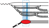
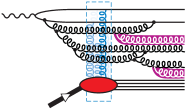
Figure 1: Generic diagrams for exclusive processes with final state interactions. In the diagrams, rapidity of gluons increases both vertically, in the final state, and horizontally, with the distance of their emission vertex to the target: To leading logarithmic accuracy, ordering in $Y$ coincides with ordering in $z^{-}$ towards the interaction region. Consequently, emissions into the final state after the interaction do not iterate: lines marked in the graph to the right are suppressed.

Reabsorption of a gluon after the interaction in the amplitude takes a form similar to a virtual correction in the JIMWLK case, but contains the soft interaction with the target, i.e. a factor $U$ per hard particle. Technically, the necessary diagrams can be constructed by introducing a “three time formalism” in which we distinguish $z^{-}=-\infty,=0$ and $=+\infty$ as the times at which the initial hard particles are created, the interaction takes place and the final state is formed respectively. The transition amplitude from $z^{-}=-\infty$ to $+\infty$ is then created in two steps: we use a shower operator to create gluons before the interaction but anticipate that some of them directly reach the final state while others will be reabsorbed after the interaction. In order to also generate the final state contributions with a shower operator, we introduce an auxiliary Gaussian “noise” $\Xi$ with the same average and correlator as in (8) and (9). Furthermore we artificially split the $U$ factors of the interaction region into two Wilson lines $W$ and $V^{\dagger}$ according to $U=WV^{\dagger}$. (One may think of them as Wilson lines extending over the intervals $[-\infty,0]$ and $[0,\infty]$, respectively, they will disappear in the final result.) We then obtain the full set of diagrams:

$$\langle{\sf U}_{\text{f}}[\Xi,\xi]{\sf U}_{\text{i}}[\Xi]\ \parbox{51.21504pt}{\includegraphics[width=51.21504pt]{alt.eps}}\ \rangle_{\Xi}$$ (14)

$$=\langle{\sf U}_{\text{f}}[\Xi,\xi]\sum\!\!\parbox{71.13188pt}{\includegraphics[width=71.13188pt]{finalstatesbefore_2.ps}}\rangle_{\Xi}=\sum\!\!\parbox{71.13188pt}{\includegraphics[width=71.13188pt]{finalstatescomplete_2.ps}}$$

where the sum is over the number of gluons and allowed insertions. The dashed line through the interaction region represents the auxiliary split of the Wilson lines into $W$ and $V^{\dagger}$ with accompanying $\Xi$ factors. The shower operators are given by

$${\sf U}_{\text{i}} [\Xi,\xi]={{\sf P}}_{Y_{2}}\exp\Big{[}i\int dY_{1}dY_{2}\,\theta(Y_{1}\!-\!Y_{2})J^{i}_{\bm{xz}}$$

$$(W^{ab}_{Y_{2},\bm{z}}\Xi^{b,i}_{Y_{2},\bm{z}}+({WV^{\dagger}})^{ab}_{Y_{2},\bm{z}}\xi^{b,i}_{Y_{2},\bm{z}})i\bar{\nabla}^{a}_{W_{Y_{1}\bm{x}}}\Big{]}$$ (15a)

$${\sf U}_{\text{f}} [\Xi,\xi]={{\sf P}}_{Y_{2}}\exp\Big{[}i\int\!\!dY_{1}dY_{2}\,\theta(Y_{1}\!-\!Y_{2})J^{i}_{\bm{xz}}$$

$$\qquad(V^{ab}_{Y_{2},\bm{z}}\Xi^{b,i}_{Y_{2},\bm{z}}+\xi^{a,i}_{Y_{2},\bm{z}})i\bar{\nabla}^{a}_{V_{Y_{1},\bm{y}}}\Big{]}\ .$$ (15b)

Eventually combining the above expression for the amplitude with the corresponding expression for the complex conjugate amplitude and differentiating w.r.t. $Y$ yields all real emission contributions to the evolution Hamiltonian as well as the interacting virtual ones. One still misses virtual lines that do not cross the interaction regions. These are again reconstructed on the level of the evolution equation. We obtain the full Hamiltonian:

$$H =u(k)H_{r}+H_{v}+H_{\bar{v}}$$ (16)

where the real gluonic corrections are produced by

$$H_{r} =-\frac{\alpha_{s}}{\pi^{2}}{\cal K}_{\bm{xzy}}\big{(}U^{ab}_{\bm{z}}i\bar{\nabla}^{a}_{U_{\bm{x}}}i\nabla^{b}_{\bar{U}_{\bm{y}}}+\bar{U}^{ab}_{\bm{z}}i\bar{\nabla}^{a}_{\bar{U}_{\bm{x}}}i\nabla^{b}_{{U}_{\bm{y}}}$$

$$\qquad\qquad\qquad+(U\bar{U}^{\dagger})^{ab}_{\bm{z}}i\bar{\nabla}^{a}_{{U}_{\bm{x}}}i\bar{\nabla}^{b}_{\bar{U}_{\bm{y}}}+i\nabla^{a}_{{U}_{\bm{x}}}i\nabla^{a}_{\bar{U}_{\bm{y}}}\big{)}\ .$$

The remaining terms correspond to virtual corrections in amplitude and complex conjugate amplitude respectively

$$H_{v}\!\!= \frac{-\alpha_{s}}{2\pi^{2}}{\cal K}_{\bm{xzy}}(i\nabla^{a}_{U_{\bm{x}}}i\nabla^{a}_{U_{\bm{y}}}\!\!+\!\!i\bar{\nabla}^{a}_{U_{\bm{x}}}i\bar{\nabla}^{a}_{U_{\bm{y}}}\!\!+\!\!2U^{ab}_{\bm{z}}i\bar{\nabla}^{a}_{U_{\bm{x}}}i\nabla^{b}_{U_{\bm{y}}})$$

$$H_{\bar{v}}\!\!= \frac{-\alpha_{s}}{2\pi^{2}}{\cal K}_{\bm{xzy}}(i\nabla^{a}_{\bar{U}_{\bm{x}}}i\nabla^{a}_{\bar{U}_{\bm{y}}}\!\!+\!\!i\bar{\nabla}^{a}_{\bar{U}_{\bm{x}}}i\bar{\nabla}^{a}_{\bar{U}_{\bm{y}}}\!\!+\!\!2\bar{U}^{ab}_{\bm{z}}i\bar{\nabla}^{a}_{\bar{U}_{\bm{x}}}i\nabla^{b}_{\bar{U}_{\bm{y}}})\ .$$

(The last terms in these expressions are the interacting parts.) The evolution equation parallels (4), with $\hat{Z}$ replaced by $\hat{Z}[U,\bar{U}]$. Note that $H_{v}$ and $H_{\bar{v}}$ taken individually have the form of the JIMWLK-Hamiltonian: $H_{v}$ is the evolution Hamiltonian for the dipole operator of the forward amplitude $\hat{N}^{0}_{\bm{xy}}=\mathop{\rm tr}\nolimits[1-U_{\bm{x}}U^{\dagger}_{\bm{y}}]/N_{c}$, which, via the optical theorem, determines the evolution of the total cross-section. Real contributions only occur outside the gap, as mandated by the factor $u(k)$. If we remove that restriction by setting $u(k)=1$, we expect complete cancellation of final state contributions and again a reduction to JIMWLK. Indeed, setting $u(k)$ to 1 and acting with (16) on the dipole operator $\hat{N}_{\bm{xy}}^{F}=\mathop{\rm tr}\nolimits[1-(U\bar{U}^{\dagger})_{\bm{x}}(U\bar{U}^{\dagger})_{\bm{y}}^{\dagger}]/N_{c}$ (which depends only on products $(U\bar{U}^{\dagger})^{(\dagger)}$), we find that the evolution Hamiltonian (16) reduces to the JIMWLK-Hamiltonian for Wilson lines $(U\bar{U}^{\dagger})$. The average over $\hat{N}^{F}_{\bm{xy}}$ then is written in terms of $\hat{Z}[U,\bar{U}]=\hat{Z}[U\bar{U}^{\dagger}]$ with evolution according to

$$\partial_{Y}\hat{Z}[U\bar{U}^{\dagger}]=-H[U\bar{U}^{\dagger}]_{\text{JIMWLK}}\hat{Z}[U\bar{U}^{\dagger}]\ ,$$ (17)

cancellation is complete.

The operators that replace $\mathop{\rm tr}\nolimits[1-U_{\bm{x}}{U}^{\dagger}_{\bm{y}}]/N_{c}$ (i.e. $\hat{N}^{F}$) in (1) for diffractive dissociation of a photon are different in- and outside the gap, the structures closely resemble the factorized results of kl . In the gap, no colored object enters the final state, thus the initial $q\bar{q}$, if in the gap, interacts with the target and emerges in a singlet state: here $\hat{N}^{D}_{\bm{xy}}$, the operator for cross sections with rapidity gaps larger than $Y_{\text{gap}}$, is a product of two traces:

$$\hat{N}^{D}_{\bm{xy}}=\hat{N}^{0}_{\bm{xy}}\cdot\hat{\bar{N}}^{0}_{\bm{yx}}=\frac{\mathop{\rm tr}\nolimits(1-U_{\bm{x}}U^{\dagger}_{\bm{y}})}{N_{c}}\frac{\mathop{\rm tr}\nolimits(1-\bar{U}^{\dagger}_{\bm{x}}\bar{U}_{\bm{y}})}{N_{c}}\ ,$$ (18)

it takes the form of the “square” of two “elastic” dipole operators corresponding to the two amplitude factors. Here, evolution of amplitude and complex conjugate are completely uncorrelated ($[H_{v},H_{\bar{v}}]=0$, $H_{r}$ is absent):

$$\hat{Z}_{Y}[U,\bar{U}]=e^{-(H_{v}+H_{\bar{v}})(Y-Y_{0})}\hat{Z}_{Y_{0}}[U,\bar{U}]\ ,$$ (19)

and one may factorize $\hat{Z}_{Y}[U,\bar{U}]\to\hat{Z}_{Y}[U]\hat{Z}_{Y}[\bar{U}]$ unless the initial condition contradicts this.

For $Y>Y_{\text{gap}}$, production of gluons in the final state is allowed and the $q\bar{q}$-pair can appear also in an octet state. Adding the octet part to (18) removes one trace:

$$\hat{N}_{\bm{xy}}^{D} =\mathop{\rm tr}\nolimits[\big{(}1-U^{\dagger}_{\bm{y}}U_{\bm{x}}\big{)}\big{(}1-\bar{U}^{\dagger}_{\bm{x}}\bar{U}_{\bm{y}}\big{)}]/{N_{c}}$$

$$=\hat{N}_{\bm{xy}}^{0}+\hat{\bar{N}}_{\bm{yx}}^{0}-\hat{N}^{F}_{\bm{xy}}\ .$$ (20)

The second line exposes further structure: With the initial conditions on evolution for $\langle\hat{N}^{D}\rangle$ imposed by (18), we find that $\langle\hat{N}^{F}\rangle$ acquires the interpretation of the cross section of events with rapidity gaps smaller than $Y_{\text{gap}}$. Following our previous reasoning we conclude that the average over the three operators in the second line of (Extension of the Color Glass Condensate Approach to Diffractive Reactions) can be described by using functionals $\hat{Z}[U]$, $\hat{Z}[\bar{U}]$ and $\hat{Z}[U\bar{U}^{\dagger}]$, with their respective evolution given by a JIMWLK-Hamiltonian. Even if additional structure in the initial conditions does not prevent these simplifications, initial conditions for the individual terms are different from each other (c.f. (18)) and the inclusive case.

The relation to the results of Kovchegov and Levin kl parallels the reduction step from JIMWLK to BK: There one observes that JIMWLK evolution of $\hat{S}_{\bm{xy}}[U]=1-\hat{N}_{\bm{xy}}=\mathop{\rm tr}\nolimits(U_{\bm{x}}U^{\dagger}_{\bm{y}})/N_{c}$ takes the simple form

$$\partial_{Y}\langle\hat{S}_{\bm{xy}}\rangle_{Y}=\frac{\alpha_{s}N_{c}}{2\pi^{2}}\int\!\!d^{2}\bm{z}\tilde{\mathcal{K}}_{\bm{xzy}}\langle\hat{S}_{\bm{xz}}\hat{S}_{\bm{zy}}-\hat{S}_{\bm{xy}}\rangle_{Y}\ ,$$ (21)

where $\tilde{\mathcal{K}}_{\bm{xzy}}=\frac{(\bm{x}-\bm{y})^{2}}{(\bm{x}-\bm{z})^{2}(\bm{z}-\bm{y})^{2}}$. Factorizing $\langle\hat{S}_{\bm{xz}}\hat{S}_{\bm{zy}}\rangle\to\langle\hat{S}_{\bm{xz}}\rangle\langle\hat{S}_{\bm{zy}}\rangle$ truncates the infinite Balitsky hierarchy and leaves us with the BK equation. For $Y>Y_{\text{gap}}$ where $\hat{N}^{D}_{\bm{xy}}=1-\hat{S}_{\bm{xy}}[U]-\hat{S}_{\bm{yx}}[\bar{U}]+\hat{S}_{\bm{xy}}[U\bar{U}^{\dagger}]$ and each $\hat{S}_{\bm{xy}}[..]$ obeys (21), the same reasoning leads to the evolution equation presented as Eq. (9) in kl . (18) and (19) imply the required initial condition $\langle\hat{N}^{D}_{\bm{xy}}\rangle(Y_{\text{gap}})=\langle\hat{N}^{0}_{\bm{xy}}\rangle^{2}(Y_{\text{gap}})$ for evolution above the gap.

To summarize: We have developed a method which allows to generalize the JIMWLK approach to a large class of exclusive observables, by simply adapting the phase space constraints. We have worked out the example of diffractive dissociation. For all generalizations it is crucial to start from IR safe observables, otherwise reconstruction of virtual contribution via real virtual cancellations must fail.

References

• (1) for a recent review see H. Weigert, Prog. Part. Nucl. Phys. 55 (2005), 461.
• (2) J. Jalilian-Marian, A. Kovner, L.D. McLerran, and H. Weigert, Phys. Rev. D55(1997) 5414;
J. Jalilian-Marian, A. Kovner, A. Leonidov, and H. Weigert, Nucl. Phys. B504 (1997) 415; Phys. Rev. D59 (1999) 014014; Phys. Rev. D59 (1999) 034007, [Erratum-ibid.Β D59, 099903 (1999)];
J. Jalilian-Marian, A. Kovner, and H. Weigert, Phys. Rev. D59 (1999) 014015;
A. Kovner, J.G. Milhano, and H. Weigert, Phys. Rev. D62 (2000) 114005;
H.Β Weigert, Nucl.Β Phys.Β  A703, 823 (2002);
E. Iancu, A. Leonidov, and L.D. McLerran, Nucl. Phys. A692 (2001) 583.
E. Ferreiro, E. Iancu, A. Leonidov, and L.D. McLerran, Nucl. Phys. A703 (2002) 489;
• (3) Y. Kovchegov and E. Levin Nucl.Β Phys. B577 (2000), 221.
• (4) I.Β Balitsky, Nucl.Β Phys. B463 (1996), 99.
• (5) Y.Β V.Β Kovchegov, Phys.Β Rev.Β  D61 (2000), 074018.
• (6) A. Banfi, G. Marchesini, and G. Smye, JHEP 0208 (2002) 006; H. Weigert, Nucl. Phys. B685 (2004) 321.
• (7) Y.Β V.Β Kovchegov and L.Β D.Β McLerran, Phys.Β Rev.Β  D60, 054025 (1999) [Erratum-ibid.Β  D62, 019901 (2000)]; A. Kovner, U. Wiedemann Phys., Rev. D64 (2001) 114002.