Abstract

The phases in a generic low-energy supersymmetric model are severely constrained by the experimental upper bounds on the electric dipole moments of the electron and the neutron. Coupled with the requirement of radiative electroweak symmetry breaking, this results in a large degree of fine tuning of the phase parameters at the unification scale. In supergravity type models, this corresponds to very highly tuned values for the phases of the bilinear Higgs coupling parameter $B$ and the universal trilinear coupling $A_{0}$. We identify a cancellation/enhancement mechanism associated with the renormalization group evolution of $B$, which, in turn, reduces such fine-tuning quite appreciably without taking recourse to very large masses for the supersymmetric partners. We find a significant amount of reduction of this fine-tuning in non-universal gaugino mass models that do not introduce any new phases.
PACS numbers:13.40.Em,04.65.+e,12.60Jv,14.20.Dh

1 Introduction

Low energy supersymmetry (SUSY)[1] has been playing a central role in the quest for physics beyond the standard model (SM). Since phenomenological consistency requires SUSY to be broken, and broken softly (so as not to reintroduce any quadratic divergence), the Lagrangian of the Minimal Supersymmetric Standard Model (MSSM)[2, 3] includes soft and gauge invariant SUSY breaking terms. While the generic MSSM Lagrangian may contain many arbitrary soft terms, specific models for SUSY breaking have been proposed that provide relationships between the MSSM parameters. Incorporating well-motivated new interactions and particles at high mass scales, such scenarios drastically reduce the large number of unknown parameters in the MSSM to only a few, thereby making the model more predictive. We will focus here only on supergravity (SUGRA)[4, 5] type of models where SUSY is considered as a local symmetry. These models incorporate a hidden sector wherein SUSY is broken, and a visible sector where the MSSM fields reside and to which the breaking is communicated by gravitational interactions. In $N=1$ SUGRA, which incorporates grand unification, one has a choice of three functions in building a model[4, 5, 6], namely the gauge kinetic energy function $f_{\alpha\beta}(z_{i})$, the Kähler potential $K(z_{i},z_{i}^{\dagger})$, and the superpotential $W(z_{i})$, where $z_{i}$ refer to matter fields. In mSUGRA, the minimal version of the model, one has a flat Kähler potential and a flat gauge kinetic energy function. The corresponding soft SUSY breaking sector is characterized by only a few parameters, normally specified at the scale of the grand unified theory (GUT) viz. $M_{G}\sim 2\times 10^{16}$ GeV[7, 8]. These are the universal gaugino mass $m_{\frac{1}{2}}$, the universal scalar mass $m_{0}$, the universal trilinear coupling $A_{0}$ and the universal bilinear coupling $B_{0}$. In addition to these, there is a superpotential parameter, namely the Higgs mixing term $\mu_{0}$. Unlike in the SM, where the breaking of the electroweak symmetry necessitates the explicit introduction of a negative valued scalar mass-squared, in a generic SUGRA model, the said breaking can be realized even for a positive mass-squared term in the bare Lagrangian, thanks to radiative corrections[4]. In other words, the renormalization of the soft SUSY breaking terms as one moves from the unification scale down to the electroweak scale automatically engenders a negative mass-squared thereby breaking the symmetry[9, 10, 11, 12]. In a similar vein, the low energy parameters of the MSSM (which are quite large in number) are obtained from only a few unification scale parameters via the renormalization group equations (RGE)[12] integrated from $M_{G}$ to the electroweak scale ($\sim M_{Z}$). The two minimization conditions for the Higgs potential then eliminate $\mu_{0}$ (except for its sign) on the one hand, and, on the other, relate $B_{0}$ to $\tan\beta$ ($\equiv\langle H_{U}\rangle/\langle H_{D}\rangle$), the ratio of Higgs vacuum expectation values. Thus mSUGRA may be characterized by $\tan\beta$, $m_{1/2}$, $m_{0}$, $A_{0}$ and sign($\mu$). With all the low energy parameters of the MSSM being generated in terms of these few parameters, one has a considerable amount of predictivity for the MSSM spectrum.

A different problem remains though, namely that of the SUSY CP violating phases. Many phases of SUGRA models can be rotated away. In an universal scenario like mSUGRA, the gaugino masses can be considered real with the result that only two combinations of phases (beyond the Cabibbo-Kobayashi-Maskawa quark mixing (CKM) phase already present in the SM) are physical. A convenient choice for the two is given by $\phi_{A_{0}}$ for $A_{0}$ (at $M_{G}$) and $\theta_{B}$ for the $B$-parameter at the electroweak scale. It should be noted though that many analyses prefer to work with $\theta_{\mu}$, the phase of $\mu$, instead of $\theta_{B}$. An advantage of this latter choice is that $\theta_{\mu_{0}}\sim\theta_{\mu}$ since $\theta_{\mu}$ does not run up to the one-loop level. These different descriptions can be understood in terms of $U(1)_{R}$ and $U(1)_{PQ}$ (Peccei-Quinn) symmetries and the choice of reparametrization invariant combinations of phases, a discussion of which may be found in Refs.[3, 14]. A selection of past analyses using $\theta_{B}$ as an input parameter may be seen in Refs.[15, 16, 17, 18, 19, 20]. Here we note that a choice of $\theta_{B}$ instead of $\theta_{\mu}$ as a phase parameter makes the entire set of input parameters to be of soft-breaking origin.

A few important points need to be noted in the context of the SUSY CP problem. The latter arises from the fact that the phases are highly constrained by the experimental limits on the electric dipole moments (EDM) of the electron and the neutron[14, 15, 16, 17, 18, 19, 21, 22]. Consequently, we are forced to admit one of the three eventualities:

1. The phase $\theta_{B}$ is very small—$O(10^{-2})$ or $O(10^{-3})$—if the superpartners are not considered to be very heavy. In addition, the phases of the $A$-parameters at the electroweak scale are also constrained. In mSUGRA with phases, the requirement of having a very small $\theta_{B}$ typically translates into a relatively large but highly fine-tuned value for ${\rm arg}(B_{0})$ (i.e., $B$ at $M_{G}$). This, in turn, constrains the phase $\phi_{A_{0}}$ of $A_{0}$, although to a somewhat lesser degree. The fact that the issue of fine-tuning in phases at the GUT scale arises out of the combined requirement of satisfying the EDM constraints and the radiative electroweak symmetry breaking was discussed in great detail in Refs.[15, 17, 16] as well as in Refs.[18, 19]. In this paper we try to focus our attention on this problem by looking at suitable models beyond mSUGRA that can have unique features in the evolution of $B$.

2. The phases are large and less fine-tuned but the sparticles are massive. Of course, fully ameliorating the SUSY CP problem in this fashion requires that the sfermions be super-massive, thereby aggravating the problem of the little mass hierarchy in the Higgs sector. We will investigate whether the amount of fine-tuning can be reduced even while one considers a lighter sparticle spectra.

3. Finally there is the possibility that the SUSY breaking parameters may have special pockets where there can be a large amount of internal cancellations between the diagrams contributing to the electric dipole moments of electron and neutron[21]. This means that phases could be large while sparticle masses are significantly light. This scenario is highly parameter dependent and clearly depends on very delicate cancellations. Hence we will not include this in our work while trying to focus on generic behaviors.

As mentioned above, we would like to address the first and the second issues in this analysis. We are particularly interested in exploring the possible role of non-universal gaugino masses (NUGM) in reducing the fine-tuning in the phase $\theta_{B_{0}}$. To quantify the latter, we consider a naturalness like measure of the form

$$\Phi=[{\Delta\theta_{B_{0}}}/{\Delta\theta_{B}}]_{\theta_{B}\rightarrow 0}.$$ (1)

A large value for $\Phi$ would mean a lesser degree of fine-tuning of $\theta_{B_{0}}$ with respect to a variation in $\theta_{B}$ satisfying the EDM constraints. The phase-derivative is evaluated at $\theta_{B}\sim 0$ with the choice being dictated by the fact that the EDM constraints force $|\theta_{B}|$ to be close to zero. Thus, this is a restrictive definition compared to the type of fine-tuning defined in Ref.[16].

We will see that the issue of such fine-tuning of phase can be addressed by focusing on scenarios where there is a large evolution of the bi-linear Higgs coupling parameter $B$ between the electroweak scale and the GUT scale. The evolution of $B$ depends on the $U(1)$ and the $SU(2)$ gaugino masses, the trilinear couplings and $\tan\beta$. Within mSUGRA, in addition to the evolution of $|B|$ being typically small, the phase $\theta_{B_{0}}$ also turns out to be quite fine-tuned (i.e. $\Phi$ tends to be small). In other words, for a given $\theta_{B_{0}}$ satisfying the EDM constraints, the variation $\Delta\theta_{B_{0}}$ that still is consistent with the constraints is generally much smaller than the variation $\Delta\theta_{B}$ allowed at the electroweak scale[15]. As we will see, the evolution in $|B|$ may be enhanced by appropriate mass relationships between the gauginos that are away from universality at $M_{G}$. At the same time, these would help in reducing the above-mentioned fine-tuning so that $\Phi$ can be significantly increased in specific NUGM scenarios.

We, however, desist from choosing an arbitrary non-universal gaugino mass scenario since that will introduce new phases[17]. As we will see in Sec.2, non-universalities in gaugino masses may originate from a non-trivial gauge kinetic energy function. The latter is a function of chiral superfields and transforms as a symmetric product of the adjoint representations of the underlying gauge group. This leaves $f_{\alpha\beta}$ with the possibility of being in one or more of several representations, one of which is the singlet. While the choice of the singlet corresponds to mSUGRA, the non-singlet representations give rise to non-universalities in the gaugino masses. It is possible to identify a suitable non-singlet representation in isolation (i.e., we will not combine a non-singlet representation with the singlet or other non-singlet representations) whose gaugino mass pattern is effective in generating a large evolution in $B$. At the same time, there will be no additional phases to worry about since the overall phase of the gaugino masses can be rotated away in a fashion similar to that in mSUGRA.

In this paper, we will analyze the consequences of a large evolution of the $B$-parameter (mostly in the presence of such non-universalities) on the CP violating phases. Here, the basic input parameters are $\tan\beta$, $m_{0}$, $m_{\frac{1}{2}}$ (providing with definite NUGM patterns), $|A_{0}|$ along with its phase $\phi_{A_{0}}$ and the phase $\theta_{B}$ of $B$ given at the electroweak scale ($\sim M_{Z}$). Note that $|B|$ at the electroweak scale is obtained via radiative electroweak symmetry breaking (REWSB) condition. Subsequently, $|B_{0}|$, the GUT scale magnitude of the $B$-parameter along with its phase $\theta_{B_{0}}$ is obtained via RGEs. We will identify broad but correlated regions of parameter space where there can be a significant degree of reduction of the phase sensitivity while going from mSUGRA to a type of NUGM models.

The paper is organized as follows. In Sec.2, we discuss the non-universal gaugino mass models. The study of the relevant contributions from different sectors in the associated RGEs of $B$ and $A$ parameters allows us to identify the non-singlet representations which provide with a large evolution in $B$. We will probe the parameter space that is suitable for reducing the amount of fine-tuning in the CP violating phases. In Sec.3, we present the numerical results for the evolution of $B$. An analysis in the absence of phases points us to the favored regions of parameter spaces. On inclusion of phases, this facilitates the identification of the regions with significantly reduced level of fine-tuning, Finally, we conclude in Sec.4.

2 Non-universal gaugino masses and enhanced evolution of $B$

Non-universality in gaugino masses may originate from a non-trivial gauge kinetic energy function $f_{\alpha\beta}$ which, in turn, is a function of the chiral superfields in the theory. The indices $\alpha,\beta$ run over the generators of the gauge group (for example, $\alpha=1,2,\dots 24$ for SU(5)). The gaugino mass matrix is given by

$$M_{\alpha\beta}=\frac{1}{4}\bar{e}^{G/2}G^{a}(G^{-1})^{b}_{a}(\partial f^{*}_{\alpha\gamma}/\partial z^{*b})f^{-1}_{\gamma\beta}$$ (2)

where $G=-\ln[\kappa^{6}WW^{*}]-\kappa^{2}K$. Here, $W$ is the superpotential, $K(z,z^{*})$ is the Kähler potential, $z^{a}$ are the complex scalar fields, and $\kappa=(8\pi G_{N})^{-\frac{1}{2}}=0.41\times 10^{-18}$ GeV^-1 with $G_{N}$ being Newton’s constant. The functions $f_{\alpha\beta}$ may have non-trivial field contents, or in other words, may contain combinations of field transforming as either singlet or non-singlet irreducible representations[24]. With the gauginos being Majorana particles, $f_{\alpha\beta}$, of necessity, must be contained in the symmetric product of the adjoint representations of the gauge group. For example, in the case of SU(5),

$$f_{\alpha\beta}\supset(24\otimes 24)_{sym}=1\oplus 24\oplus 75\oplus 200\ .$$ (3)

For the singlet case, one has $f_{\alpha\beta}=\delta_{\alpha\beta}$ which indeed leads to universality of gaugino masses. Similarly, the non-singlet representations will give rise to non-universal gaugino masses.

In general $M_{i}(M_{G})=m_{\frac{1}{2}}\sum_{r}C_{r}n_{i}^{r}$, where $C_{r}$’s give the relative weights of each contributing representation and $n_{i}^{r}$, for the subgroup $i$, are essentially the Clebsch-Gordan coefficients corresponding to the breaking by the adjoint Higgs field[24, 25, 26]. For the case of $SU(5)$, the coefficients $n_{i}^{r}$ are displayed in Table 1. Clearly, the non-singlet representations have characteristic mass relationships for the gaugino masses at the GUT scale. Past analyses exploring various phenomenological implications of such non-universality may be found in Refs.[24, 25, 27, 28, 29].

As we shall argue later, the adjoint representation $r=24$ for $f_{\alpha\beta}$ (NUGM:24 in the notation of Table 1) is the most interesting one in the context of the present investigation. Consequently, we will analyze this case in isolation, or, in other words, assume that the sole contribution to $f_{\alpha\beta}$ is from a 24-plet structure. Apart from reducing the number of free parameters, this has the additional advantage that no new phase degree of freedom for the gaugino masses is introduced. With the gaugino mass ratios at the GUT scale now being given by $M_{3}(M_{G}):M_{2}(M_{G}):M_{1}(M_{G})=1:-3/2:-1/2$, for a positive gluino mass, the other two gaugino mass parameters are negative, a signature different from mSUGRA. This indeed would turn out to be useful in our quest. As mentioned earlier, we only consider either $C_{1}=1$ (mSUGRA) or $C_{24}=1$ (NUGM:24) with all other $C_{r}$’s assumed to be zero.

$r$	Label	$M^{G}_{3}$	$M^{G}_{2}$	$M^{G}_{1}$
1	mSUGRA	1	1	1
24	NUGM:24	2	$-3$	$-1$
75	NUGM:75	1	3	$-5$
200	NUGM:200	1	2	10

Table 1: The coefficients $n_{i}^{r}$ as pertaining to the $SU(3)$, $SU(2)$ and $U(1)$ gaugino masses at the GUT scale for different representations of $SU(5)$.

An analogous analysis with SO(10) as the underlying gauge group is also possible[30, 29], though we will not investigate it in this paper. Similar to Eq.3 here, one has $(45\times 45)_{sym}=1+54+210+770$. If the symmetry breaking pattern is $SO(10)\rightarrow SU(4)\times SU(2)\times SU(2)\rightarrow SU(3)\times SU(2)\times U(1)$, one finds from the $54$-plet that $M_{3}(M_{G}):M_{2}(M_{G}):M_{1}(M_{G})=1:-3/2:-1$. This pattern is quite similar to NUGM:24 as can be ascertained from Table 1. We would like to comment at this point that, in general, such non-universal gaugino mass scenarios change the gauge coupling unification conditions[24, 26]. However, it is still possible to find specific conditions[31, 24] under which the usual gauge coupling unification condition remains unaltered and we consider this in our work. Note though that our results are quite robust and have very little dependence on the exact details of the spectrum.

2.1 Nature of evolution of $B$ with real parameters

We now identify the differences between mSUGRA and NUGM:24 in regard to the evolution of the $B$-parameter in the absence of CP violating SUSY phases. This, in turn, will help us in understanding the evolution of $\theta_{B}$ upon the inclusion of the phases (see Refs.[17, 18, 19, 20] for past analyses discussing phase evolutions). Note that $\mu^{2}$ and $B$ are determined via the REWSB condition, viz.

$$\begin{array}[]{rcl}|\mu|^{2}&=&\displaystyle-\frac{1}{2}M^{2}_{Z}+\frac{m_{H_{D}}^{2}-m_{H_{U}}^{2}\tan^{2}\beta}{\tan^{2}\beta-1}+\frac{\Sigma_{1}-\Sigma_{2}\tan^{2}\beta}{\tan^{2}\beta-1}\\[8.61108pt] \sin(2\beta)&=&2|B\mu|/(m_{H_{D}}^{2}+m_{H_{U}}^{2}+2\mu^{2}+\Sigma_{1}+\Sigma_{2})\ ,\end{array}$$ (4)

where $\Sigma_{i}$ represent the one-loop corrections [32, 33]. The Higgs scalar mass parameters $m_{H_{D}}$ and $m_{H_{U}}$, and thereby $\mu^{2}$ and $B$ depend quite strongly on $m_{0}$ as well as on $m_{\frac{1}{2}}$. To one-loop order, the running of the $B$ parameter has two additive components, the first proportional to the gaugino masses and the second depending on a combination of the trilinear couplings and the Yukawa couplings [17, 12], namely,

$${\frac{dB}{{dt}}}=(3\tilde{\alpha}_{2}{\tilde{m}_{2}}+\frac{3}{5}\tilde{\alpha}_{1}{\tilde{m}_{1}})+(3Y_{t}A_{t}+3Y_{b}A_{b}+Y_{\tau}A_{\tau})\ ,$$ (5)

where $t=ln(M_{G}^{2}/Q^{2})$ with $Q$ being the renormalization scale. $\tilde{\alpha}_{i}=\alpha_{i}/(4\pi)$ are the scaled gauge coupling constants (with $\alpha_{1}=\frac{5}{3}\alpha_{Y}$) and $\tilde{m}_{i}$ for $i=1,2,3$ are the running gaugino masses. Furthermore, $Y_{i}$ represent the squared Yukawa couplings, e.g, $Y_{t}\equiv y_{t}^{2}/(4\pi)^{2}$ where $y_{t}$ is the top Yukawa coupling. In a similar vein, the evolution of the trilinear terms is given by

$$\begin{array}[]{rcl}\displaystyle{\frac{dA_{t}}{{dt}}}&=&\displaystyle-(\frac{16}{3}\tilde{\alpha}_{3}{\tilde{m}_{3}}+3\tilde{\alpha}_{2}{\tilde{m}_{2}}+\frac{13}{15}\tilde{\alpha}_{1}{\tilde{m}_{1}})-6Y_{t}A_{t}-Y_{b}A_{b}\\[6.45831pt] \displaystyle{\frac{dA_{b}}{{dt}}}&=&\displaystyle-(\frac{16}{3}\tilde{\alpha}_{3}{\tilde{m}_{3}}+3\tilde{\alpha}_{2}{\tilde{m}_{2}}+\frac{7}{15}\tilde{\alpha}_{1}{\tilde{m}_{1}})-Y_{t}A_{t}-6Y_{b}A_{b}-Y_{\tau}A_{\tau}\\[6.45831pt] \displaystyle{\frac{dA_{\tau}}{{dt}}}&=&\displaystyle-(3\tilde{\alpha}_{2}{\tilde{m}_{2}}+\frac{9}{5}\tilde{\alpha}_{1}{\tilde{m}_{1}})-3Y_{b}A_{b}-4Y_{\tau}A_{\tau}\ .\end{array}$$ (6)

For small $\tan\beta$, the contributions from the bottom quark and tau Yukawa couplings $y_{b}$ and $y_{\tau}$ may be neglected, and the RGEs approximately integrated to obtain [15]

$$B-B_{0}\simeq\frac{D_{0}(t)-1}{2}\,A_{0}-C(t)\,m_{\frac{1}{2}}\ ,$$ (7)

where $D_{0}(t)\equiv 1-6Y(t)F(t)/E(t)$ with $t$ corresponding to the electroweak scale. The functions $E(t)$ and $F(t)$ encapsulate the running of the gauge coupling constants, viz,

$$\begin{array}[]{rcl}E(t)&=&\displaystyle(1+\beta_{3}t)^{16/(3b_{3})}(1+\beta_{2}t)^{3/b_{2}}(1+\beta_{1}t)^{13/(15b_{1})}\\[8.61108pt] F(t)&\equiv&\displaystyle\int_{0}^{t}E(t^{\prime})dt^{\prime}\end{array}$$

where $\beta_{i}=b_{i}{\tilde{\alpha}}_{i}(0)$ and $(b_{1},b_{2},b_{3})=(33/5,1,-3)$ are the coefficients in the respective one-loop beta-functions. Of course, unification imposes the boundary condition that $\alpha_{i}(0)=\alpha_{G}\sim 1/24$. At the top mass scale ($Q=m_{t}$), $D_{0}\simeq 1-(m_{t}/200\sin\beta)^{2}\mathrel{\mathchoice{\vbox{\offinterlineskip\halign{$\m@th\displaystyle\hfil#\hfil$\cr<\crcr\sim\crcr} }}{\vbox{\offinterlineskip\halign{$\m@th\textstyle\hfil#\hfil$\cr<\crcr\sim\crcr} }}{\vbox{\offinterlineskip\halign{$\m@th\scriptstyle\hfil#\hfil$\cr<\crcr\sim\crcr} }}{\vbox{\offinterlineskip\halign{$\m@th\scriptscriptstyle\hfil#\hfil$\cr<\crcr\sim\crcr} }}}0.2$ is indeed a very good approximation. The function $C(t)$, in Eq.7, on the other hand, is given by

$$C(t)=-\frac{1}{2}(1-D_{0}){H_{3}\over F}+\left(3h_{2}+\frac{3}{5}h_{1}\right){\alpha_{G}\over{4\pi}}\ ,$$ (8)

where

$$\begin{array}[]{rcl}h_{i}(t)&\equiv&\displaystyle\frac{t}{(1+\beta_{i}t)}\\[8.61108pt] H_{3}(t)&\equiv&\displaystyle\int_{0}^{t}{E(t^{\prime})H_{2}(t^{\prime})}dt^{\prime}\\[8.61108pt] H_{2}(t)&\equiv&\displaystyle{\tilde{\alpha}}(0)\left({\frac{16}{3}}h_{3}+3h_{2}+{\frac{13}{15}}h_{1}\right)\ .\end{array}$$

For the generic (NUGM) case, the above results remain the same except that [25]

$$h_{i}(t)\longrightarrow{\tilde{h}}_{i}(t)\equiv h_{i}(t)\,{\frac{{\tilde{m}}_{i}(0)}{m_{\frac{1}{2}}}}\ .$$ (9)

Note that, in $dB/dt$, the gaugino contribution is positive for mSUGRA, but negative for NUGM:24. Thus, it is useful to understand the nature of evolution of trilinear couplings in either scenario so as to evaluate their role in the evolution of $B$. For the mSUGRA case, the gaugino contributions to $dA_{i}/dt$ are always negative (vide Eq.6). Hence, it is obvious that if $A_{0}$ not be too large, then $A_{i}$ would typically turn negative by the electroweak scale. In fact, the large gluino contributions render both $A_{t}$ and $A_{b}$ negative well above the electroweak scale. This implies, that in this case (mSUGRA), the two pieces in $dB/dt$ would tend to cancel each other, an effect also manifested by the smallness of $C$ in Eq.7. In turn, this leads to a small value for $\Delta B\equiv|B_{0}-B|$ in mSUGRA.

Comparing the evolution of the trilinear terms in NUGM:24 with that in mSUGRA, it turns out that a qualitative difference arises only in the case of $A_{\tau}$, while for $A_{t}$ and $A_{b}$ the difference between the scenarios is only a quantitative one. This is easy to understand given the overwhelming dominance, in the last two cases, of the gluino contribution over those from the electroweak gauginos. Specifically, for $A_{0}=0$, $A_{\tau}$ at the weak scale comes to be negative for mSUGRA while it is positive (with usually a larger magnitude) for NUGM:24. Given the relative weights of the $A_{i}$ terms in Eq.5, it is thus quite apparent that the total contribution from the trilinear couplings to the evolution of $B$ is quite similar in the two models. On the other hand, since the signs of ${\tilde{m}_{1,2}}$ are reversed in NUGM:24, the aforementioned cancellations in $dB/dt$ would no longer be operative; rather, the different contributions would enhance each other leading to a large $\Delta B$. This is the very reason why we choose to concentrate on models like NUGM:24. We note in passing that although the RGE for $B$ does not explicitly include the SU(3) gaugino mass, it implicitly depends on the latter via the contributions from trilinear couplings.

We now discuss the dependence of $B$ and $B_{0}$ on $m_{0}$ and the other parameters. Being obtained from the REWSB condition of Eq.4, $B$ (and hence $B_{0}$) evidently depends on $m_{0}$ quite strongly. The structure of Eq.5 suggests that, to one-loop order, $\Delta B$ should not depend on $m_{0}$. However, a subsidiary dependence arises through the determination of the scale at which the minimizations of Higgs potential (i.e. REWSB) is to be performed. Canonically, this scale is determined by demanding that the contribution, to $\mu^{2}$, of the 1-loop correction terms of the effective potential be small. In our analysis this scale is approximately halfway between the lowest and highest mass of the spectra and, generally, is not very far from the average stop mass scale $\sqrt{m_{{\tilde{t}}_{1}}m_{{\tilde{t}}_{2}}}$ (see Ref.[34]). Since this scale does depend on $m_{0}$, it leads to a small dependence in $\Delta B$ as well by virtue of being a limit of integration for the RGEs.

2.2 Incorporating CP violating phases: $|B_{0}|/|B|$ and phase naturalness measure $\Phi$

Even on inclusion of phases for the $A$ and $B$ parameters, the RGEs formally remain the same as in Eqs.(5&6). The evolution of the phases can then be extracted by comparing the real and imaginary parts of the said equations. Clearly, unlike in the case of the real parts, the imaginary parts of the beta functions for $A$’s and $B$ do not depend on the gaugino masses and hence there is no cancellation between the different contributions. Furthermore, even a vanishing $\theta_{B_{0}}$ can lead to a non-zero $\theta_{B}$ provided $A_{0}$ has a non-trivial phase. For example, in the small $\tan\beta$ limit, the explicit analytical solution gives

$$\begin{array}[]{rcl}|B|\sin\theta_{B}&=&\displaystyle|B_{0}|\sin\theta_{B_{0}}-\frac{1}{2}(1-D_{0})|A_{0}|\sin\phi_{A_{0}}\\[8.61108pt] |B|\cos\theta_{B}&=&\displaystyle|B_{0}|\cos\theta_{B_{0}}-\frac{1}{2}(1-D_{0})|A_{0}|\cos\phi_{A_{0}}-Cm_{\frac{1}{2}}\ .\end{array}$$ (10)

We examine now the interdependence between the phases, their evolution (also see Ref.[15]) and the phase sensitivity $\Phi$ for different values of $\tan\beta$ and other parameters both within mSUGRA as well as NUGM:24. As we have already mentioned, the EDM constraints limit $\theta_{B}$ to be tiny ($\mathrel{\mathchoice{\vbox{\offinterlineskip\halign{$\m@th\displaystyle\hfil#\hfil$\cr<\crcr\sim\crcr} }}{\vbox{\offinterlineskip\halign{$\m@th\textstyle\hfil#\hfil$\cr<\crcr\sim\crcr} }}{\vbox{\offinterlineskip\halign{$\m@th\scriptstyle\hfil#\hfil$\cr<\crcr\sim\crcr} }}{\vbox{\offinterlineskip\halign{$\m@th\scriptscriptstyle\hfil#\hfil$\cr<\crcr\sim\crcr} }}}0.1$, and typically much smaller). Now, if either of $|A_{0}|$ or $\phi_{A_{0}}$ is small (actually, if $|A_{0}|\sin\phi_{A_{0}}\ll|B|\sin\theta_{B}$), then $\theta_{B_{0}}$ would be determined essentially by $|B|$, $|B_{0}|$ and $\theta_{B}$. In this case, $\phi_{A_{0}}$ would be quite unconstrained. The dependence on $\tan\beta$ is crucial and is best understood by considering the two opposite limits, namely small and large values:

• For a small $\tan\beta$ ($\mathrel{\mathchoice{\vbox{\offinterlineskip\halign{$\m@th\displaystyle\hfil#\hfil$\cr<\crcr\sim\crcr} }}{\vbox{\offinterlineskip\halign{$\m@th\textstyle\hfil#\hfil$\cr<\crcr\sim\crcr} }}{\vbox{\offinterlineskip\halign{$\m@th\scriptstyle\hfil#\hfil$\cr<\crcr\sim\crcr} }}{\vbox{\offinterlineskip\halign{$\m@th\scriptscriptstyle\hfil#\hfil$\cr<\crcr\sim\crcr} }}}5$ or so), $\sin 2\beta$ is large, and therefore $|B|$ is appreciably large (see Eq.4). Within mSUGRA, for not too large a value of $|A_{0}|$, the GUT scale value $|B_{0}|$ is then quite comparable to $|B|$. This can be understood by recognizing the cancellations between the various terms in Eq.8 that keeps $C$ small and thereby keep $B-B_{0}$ relatively small (courtesy Eq.7). Consequently, in such a scenario, $\theta_{B_{0}}$ is not too different from $\theta_{B}$. This remains true even for $\phi_{A_{0}}=\pi/2$ which maximizes the EDM values[22].

  On the contrary, the situation in NUGM:24 is quite different. Here, a larger difference between $|B|$ and $|B_{0}|$ is generated by the enhancement in $C$. Consequently, $\theta_{B_{0}}$ becomes appreciably different from (and numerically larger than) $\theta_{B}$.

• For a large value of $\tan\beta$, on the other hand, $\sin\,2\beta$ is quite small. Thus, unless $|\mu|$ is extremely tiny (as happens, for example, in hyperbolic branch/focus point[34, 35] scenarios), $|B|$ is constrained to be small and has only sub-dominant influence on the evolution of $\theta_{B}$. This, in turn, implies that the value of $\theta_{B_{0}}$ becomes strongly correlated with that of $\phi_{A_{0}}$. In other words, a high degree of fine-tuning in one will necessitate a similar degree of fine-tuning in the other.

We now focus on the issue of phase sensitivity. As Eq.10 suggests, the range allowed to $\theta_{B}$ (i.e. $\Delta\theta_{B}$) imposes rather strong limits in the $\theta_{B_{0}}$–$\phi_{A_{0}}$ plane. Adopting the measure of phase naturalness $\Phi$ (as espoused in Eq.1), one may estimate, from Eq.10, the amount of fine-tuning associated with the phase $\theta_{B_{0}}$. Now, as the RGEs suggest, the implicit dependence of $\Phi$ on $A_{0}$ occurs primarily through the dependence of $B_{0}$ itself on $A_{0}$. Thus, to the leading order, one has an approximate relation of the form[15]

$$\Phi\sim|B\,/\,B_{0}|\ .$$ (11)

We would like to point out that although the above simplification (as also those of neglecting $y_{b}$ and $y_{\tau}$) is quite illustrative, we do not take recourse to it. Rather we solve the complete set of RGEs numerically and also compute $\Phi$ numerically directly from its definition (Eq.1).

Note that, as obtained from Eq.1 and the first of Eqs.10, the measure $\Phi$ actually involves a factor of $\cos\theta_{B_{0}}$ in the denominator. This causes $\Phi$ to be very large when $\theta_{B_{0}}$ is close to $\pi/2$, as also a change of sign for $\Phi$ when $\theta_{B_{0}}$ crosses $\pi/2$. We will see that this is indeed the case for NUGM:24 where $\theta_{B_{0}}$ can easily cross $\pi/2$ owing to a large degree of phase evolution. In the mSUGRA scenario, on the other hand, such a feature rarely appears.

As we have already discussed, mSUGRA is associated with a relatively small degree of evolution in $B$, and hence $|B|\sim|B_{0}|$. This leads to a low value of $\Phi\sim 1$ or, equivalently, to a high degree of fine-tuning in $\theta_{B_{0}}$ . On the other hand, a non-universal gaugino mass scenario like NUGM:24 can provide us with a large evolution of $|B|$. This, of course, can generate either $|B\,/\,B_{0}|\ll 1$ or $|B\,/\,B_{0}|\gg 1$. The parameter space corresponding to the latter case (which is typically satisfied better for smaller $\tan\beta$ zones) reduces fine-tuning in $\theta_{B_{0}}$. We will see that the said reduction can be as large as a factor of 10 to 20 compared to mSUGRA. And finally, the very same large evolution of $|B|$ also implies that $|B_{0}|\sim 0$ could be a possibility within such scenarios. In NUGM:24 where the evolution of $B$ is large, the above reduction of $|B_{0}|$ toward zero is possible when $|B|$ is large i.e. when $\tan\beta$ is small. In mSUGRA too this is possible, but only to a limited degree, as the aforesaid evolution is smaller in extent. So $|B|$ needs to be closer to zero in order to have a tiny $|B_{0}|$. In this sense, a requirement of a smaller $|B|$ would then favor large values of $\tan\beta$ for mSUGRA. This we explore numerically in the next section.

3 Results: Degree of $B$-evolution and phase sensitivity for mSUGRA and NUGM:24

We show our numerical results in two stages. To begin with, we examine the difference between the evolution of $B$ in mSUGRA and the NUGM:24 scenarios in the absence of any phases. Building on the lessons drawn from this exercise, we investigate next the core issue at hand, namely the behavior of the phase naturalness measure $\Phi$ in each of the scenarios and the differences therein.

3.1 Results in the absence of CP violating phases

Focusing first on mSUGRA, we begin with the value of $B$ as determined, by the REWSB conditions, in terms of the other parameters of the model, viz, $m_{0}$, $m_{\frac{1}{2}}$, $A_{0}$ and $\tan\beta$. This study, coupled with that for the derived value at the GUT scale, $B_{0}$, would serve to indicate the regions of the parameter space for which the phase sensitivity can be significantly reduced.

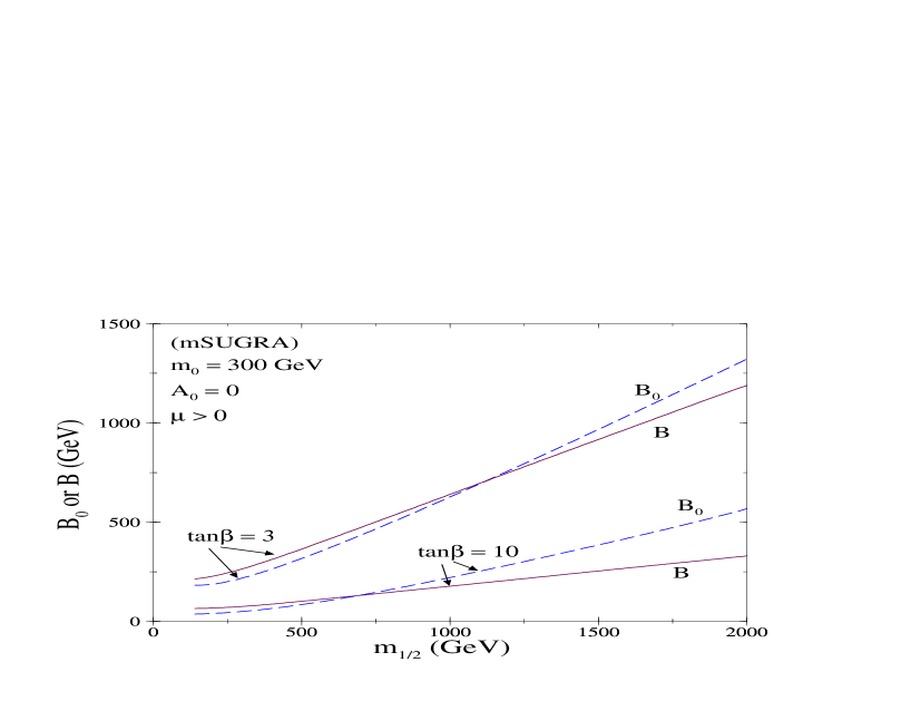
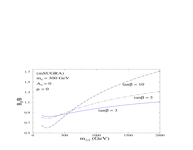
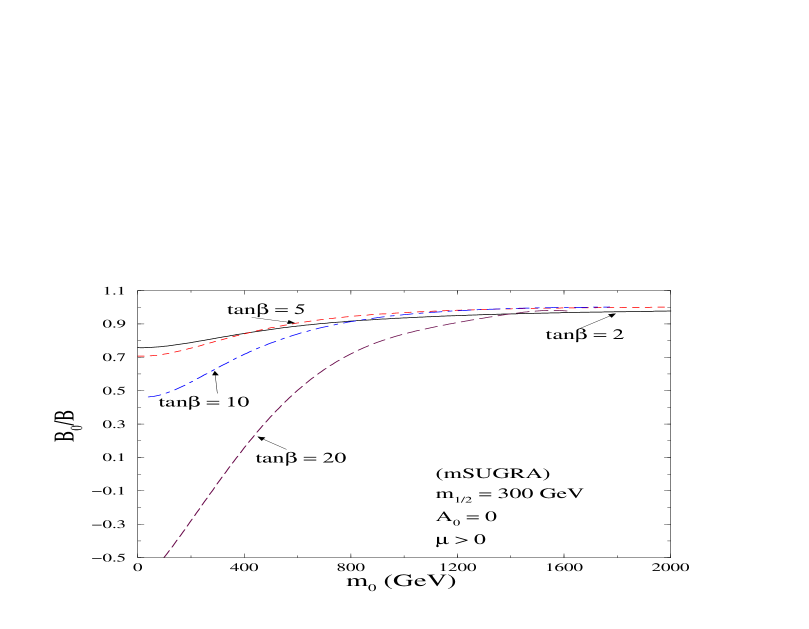
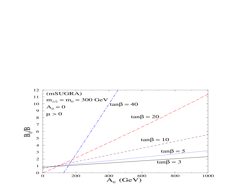
Figure 1: (a) The dependence of $B$ and $B_{0}$ on $m_{\frac{1}{2}}$ in mSUGRA with the other parameters fixed as shown. (b,c,d) The dependence of the ratio $B_{0}/B$ on $m_{\frac{1}{2}}$, $m_{0}$ and $A_{0}$ respectively, keeping the other parameters fixed.

Fig.1 shows the variation of $B$ and correspondingly $B_{0}$ with respect to $m_{\frac{1}{2}}$. With an illustrative choice of parameters, viz. $m_{0}=300$ GeV, $A_{0}=0$ and $\mu>0$, we exhibit our results for $\tan\beta=3$ and $10$. One finds that $B$, determined through the REWSB condition, is almost linear with $m_{\frac{1}{2}}$. The dependence on $\tan\beta$, on the other hand, is quite nonlinear; but as already touched upon in the previous section, the REWSB condition implies that, for a given $m_{\frac{1}{2}}$, $B$ decreases with increase in $\tan\beta$. As for the evolution of $B$, we find that $B_{0}\sim B$ unless $m_{\frac{1}{2}}$ is quite large. This is reflective of the aforementioned cancellations between the gaugino and trilinear terms of Eq.5 in mSUGRA. For our choice of $A_{0}=0$, this is same as the cancellations between the terms of $C$ of Eq.8. Once $m_{\frac{1}{2}}$ becomes large, the contributions from the gaugino part of Eq.5 dominates and the cancellations are no longer as effective. This causes $B_{0}$ to supersede $B$ as is shown in Fig.1.

The information regarding the evolution of $B$ can also be parametrized in terms of the ratio $B_{0}/B$ and this is displayed in Fig.1 as a function of $m_{\frac{1}{2}}$. This ratio is of particular interest on account of its relatively straightforward relation with the phase naturalness measure $\Phi$ (note that $\Phi\sim|B\,/\,B_{0}|$). As could have been guessed from Fig.1 itself, the variation with $m_{\frac{1}{2}}$ is nearly monotonic. The shallow dip at small $m_{\frac{1}{2}}$ values is a consequence of the variation in the degree of cancellation between contributions to $dB/dt$ and is difficult to see analytically from the leading terms alone. For large $m_{\frac{1}{2}}$, the ratio $B_{0}/B$ is seen to increase with $\tan\beta$, while for small $m_{\frac{1}{2}}$ the behavior is opposite. This, within mSUGRA, indicates that a small value of $m_{\frac{1}{2}}$, coupled with a large $\tan\beta$ seems to be best suited for achieving a low degree of fine-tuning in the phases.

In Fig.1, we display the dependence of the same ratio on $m_{0}$. While the behavior may seem intriguing at first, note that $B$ depends on $m_{0}$ only via the requirement of REWSB. As Fig.1 has already shown us, for the reference value of $m_{\frac{1}{2}}=300\rm~{}GeV$, $B_{0}$ is typically somewhat smaller than $B$. Now, $B$ grows smaller as $m_{0}$ decreases. Thus, for small $m_{0}$ and large $\tan\beta$, $B$ can be very small and the aforesaid evolution implies that $B_{0}$ would have been negative. On the other hand, for large $m_{0}$ values, $B$ is large and thus the relatively small evolution leaves the ratio $B_{0}/B$ very close to unity.

The dependence of $B_{0}/B$ on the trilinear coupling parameter $A_{0}$ is quite linear (Fig.1). This, again, can be deduced from Eq.7 where fixing $\tan\beta$, $m_{\frac{1}{2}}$ and $m_{0}$ will give rise to a linear relation between $B_{0}/B$ and $A_{0}$. Note that progressively larger values for $\tan\beta$ increases the importance of the trilinear term contributions to $dB/dt$, thereby increasing the slope of the curve.

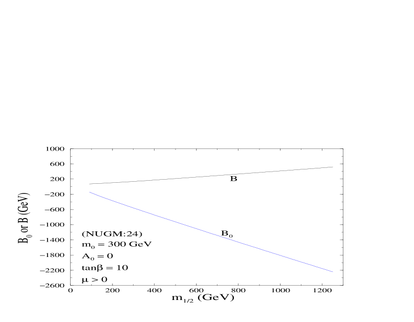
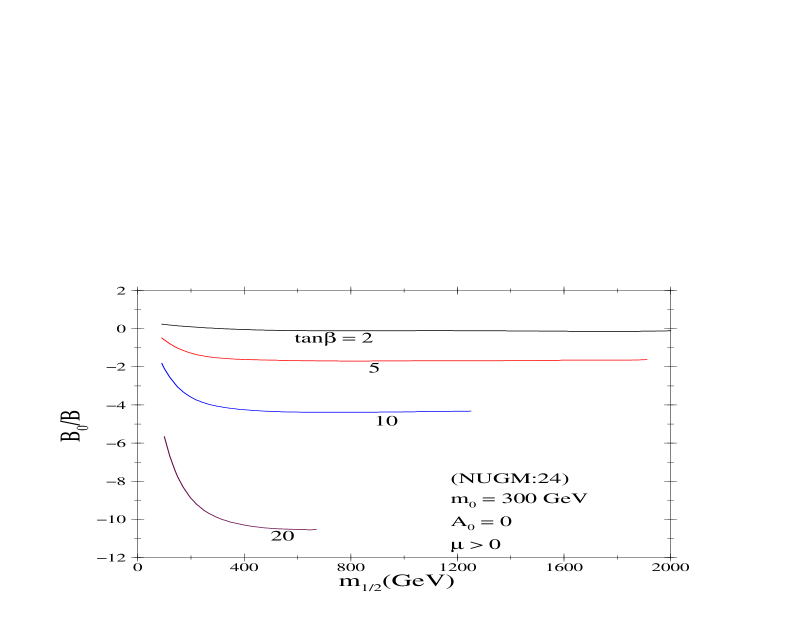
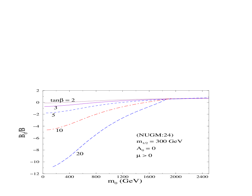
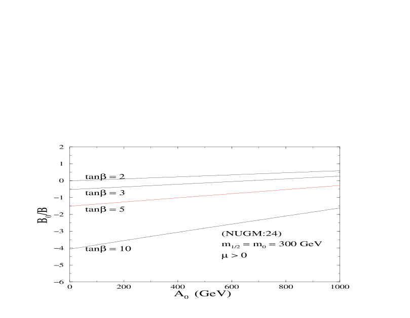
Figure 2: As in Fig.1, but for NUGM:24 instead.

We now repeat the analysis for the case of NUGM:24 choosing $A_{0}=0$ as before. However, since the sign of the electroweak gaugino mass parameters are now reversed, the gaugino contribution to Eq.5 would now enhance the trilinear contribution instead of cancelling it. And since the sign inversion affects only the sub-dominant contributions to the evolution of $A_{t,b}$, the latter remain close to their mSUGRA values with the result that the total trilinear contribution to $dB/dt$ suffers only a small relative change. The result is then a monotonic decrease of $B_{0}$ with an increase in $m_{\frac{1}{2}}$, and hence, in an appreciably large amount of evolution (Fig.2).

A further consequence is that the ratio $B_{0}/B$ too is monotonic in $m_{\frac{1}{2}}$ (Fig.2). The slope though decreases with $m_{\frac{1}{2}}$, leading to a flat behavior for moderately large $m_{\frac{1}{2}}$ values. This can be understood by realizing that, apart from $B$ being approximately linear in $m_{\frac{1}{2}}$ $\Delta B$ too is approximately linear especially for large $m_{\frac{1}{2}}$. While the steep slope for small $m_{\frac{1}{2}}$ might seem intriguing given the almost linear behavior of both $B$ and $B_{0}$ in Fig.2, it should be noted that $B$ is very small for such $m_{\frac{1}{2}}$ and consequently any departure from linearity would be magnified in the ratio. That the slopes at small $m_{\frac{1}{2}}$ values grow with $\tan\beta$ is understandable too, as for larger $\tan\beta$, the trilinear term contributions to $\Delta B$ assume greater significance.

The abrupt ending of the curves, especially for larger $\tan\beta$ values might seem curious. However, note that $A_{\tau}$ is appreciably larger in NUGM:24 than in mSUGRA (see Sec.2.1). This leads to a rapid suppression of $m_{{\tilde{\tau}}_{1}}$, the mass of the lighter stau. While the latter also sees an enhancement on account of the $SU(2)$ gaugino mass being significantly larger in NUGM:24 in comparison that within mSUGRA for an identical value of $m_{\frac{1}{2}}$, this effect is sub-dominant. Consequently, for such parameter values, the lighter stau would have a mass smaller than the lightest of the neutralinos thereby becoming the lightest supersymmetric particle. Since this is phenomenologically unacceptable, such regions of the parameter space have to be discarded. Note though that the extent of the allowed parameter range in the $m_{\frac{1}{2}}$–$\tan\beta$ plane does depend on the value of $m_{0}$.

Fig.2 displays $B_{0}/B$ for different values of $\tan\beta$ as $m_{0}$ is varied. As discussed before, $B$ increases with increase of $m_{0}$ and diminishes with increasing $\tan\beta$. For most of the region (except when $m_{0}$ is large and $\tan\beta$ quite small) the ratio can be large and negative because of a large degree of evolution of $B$ in NUGM:24. For larger $\tan\beta$, $B$ itself is much smaller. Hence a large evolution results into a large negative $B_{0}$. On the other hand, a larger value for $m_{0}$ pushes $B$ higher and $B_{0}$ would then be dragged down to a value near zero. Additionally, we like to clarify that the larger $\tan\beta$ curves really end near 2 TeV or so in Fig.2 because of the REWSB requirement. This is unlike the smaller $\tan\beta$ contours that span the entire $m_{0}$ range displayed.

As for the dependence on $A_{0}$ (see Fig.2), the relationship is once again linear, as predicted by Eq.7, for either of the two models under discussion.

3.2 Evolution of CP violating phases

Having analyzed the simple case of $\theta_{B}=\phi_{A_{0}}=0$, we may now consider the effect of phases. To start with, we continue to maintain $\theta_{B}=0$, but now consider $\phi_{A_{0}}=\pi/2$, or, in other words, a maximal phase in the trilinear coupling. This choice maximizes the EDM values[22]. To study the generic features and compare with the results of Sec.3.1, we first choose a relatively small value of $|A_{0}|$ ($=100$ GeV). Thus, $\Re(A_{i})$ and $\Re(B$) would not be very different from the analysis of Sec.3.1 because of the absence of any phase in the gaugino parts of Eqns.(5 & 6) and the smallness of $|A_{0}|$. With this choice of inputs, the only contributions to $d\Im(B)/dt$ or $d\Im(A_{i})/dt$ arise from $\Im(A_{i})$ themselves, and hence there is no occasion for cancellations/enhancements unlike in the case for the real parts. In addition, the effect of $\phi_{A_{0}}$ on $|B_{0}|$ would be limited even for maximal $\phi_{A_{0}}$ unless $|A_{0}|$ is quite large. This is reflected by Figs.3, wherein we display the variation of both $|B|$ and $|B_{0}|$ with $m_{\frac{1}{2}}$ for either model. The results are seen to be consistent with the no-phase cases of Fig.1 and Fig.2.

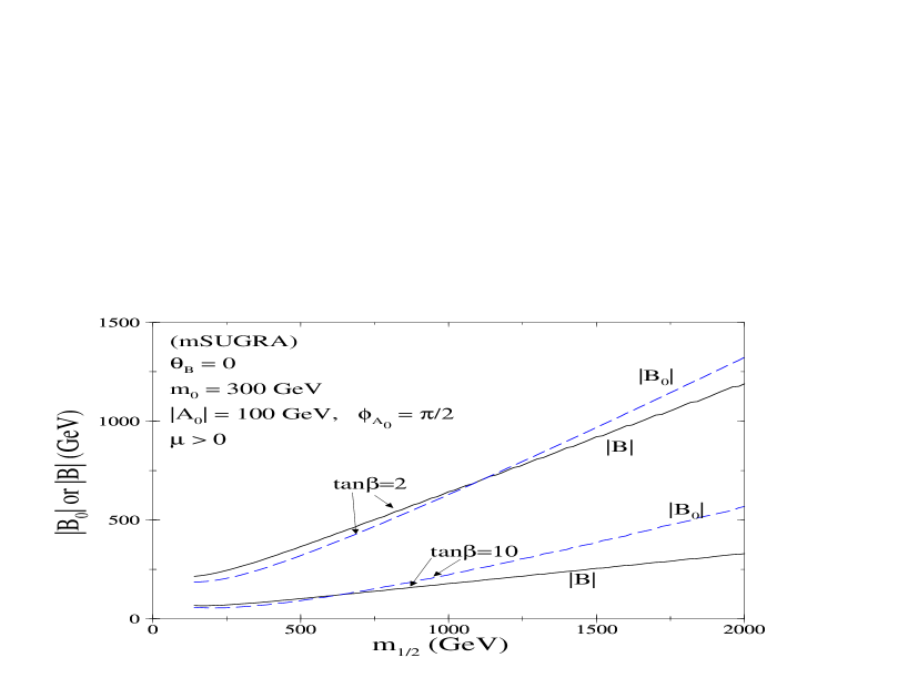
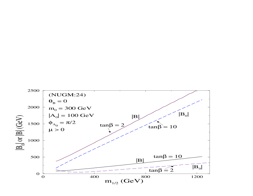
Figure 3: $B$ and $B_{0}$ vs $m_{\frac{1}{2}}$ for the displayed parameters with non-zero $\phi_{A_{0}}$ in mSUGRA and in NUGM:24.

We now invoke a non-zero $\theta_{B}$ and analyze the resulting evolution of the same from the electroweak scale to the GUT-scale. In Figs.4, we display this for both mSUGRA and NUGM:24, and in each case for two values of $\tan\beta$, namely 3 and 10. Again, for illustrative purposes, we choose, for the other relevant parameters, $m_{0}=100$ GeV, $m_{\frac{1}{2}}=300$ GeV and $|A_{0}|=300$ GeV with $\phi_{A_{0}}=\pi/2$. Although the constraints from the EDM measurements restrict $|\theta_{B}|$ to very small values ($\mathrel{\mathchoice{\vbox{\offinterlineskip\halign{$\m@th\displaystyle\hfil#\hfil$\cr<\crcr\sim\crcr} }}{\vbox{\offinterlineskip\halign{$\m@th\textstyle\hfil#\hfil$\cr<\crcr\sim\crcr} }}{\vbox{\offinterlineskip\halign{$\m@th\scriptstyle\hfil#\hfil$\cr<\crcr\sim\crcr} }}{\vbox{\offinterlineskip\halign{$\m@th\scriptscriptstyle\hfil#\hfil$\cr<\crcr\sim\crcr} }}}{\cal O}(10^{-2})$), we display the functional dependence for a wider range of $\theta_{B}$. The apparent discontinuities for the NUGM:24 curves are not physical and have only been occasioned by the choice for the domain of $\theta_{B_{0}}$, namely $[-\pi,\pi]$. Clearly, the amount of phase evolution in NUGM:24 is seen to be higher than that in mSUGRA.

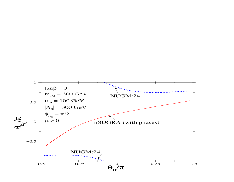
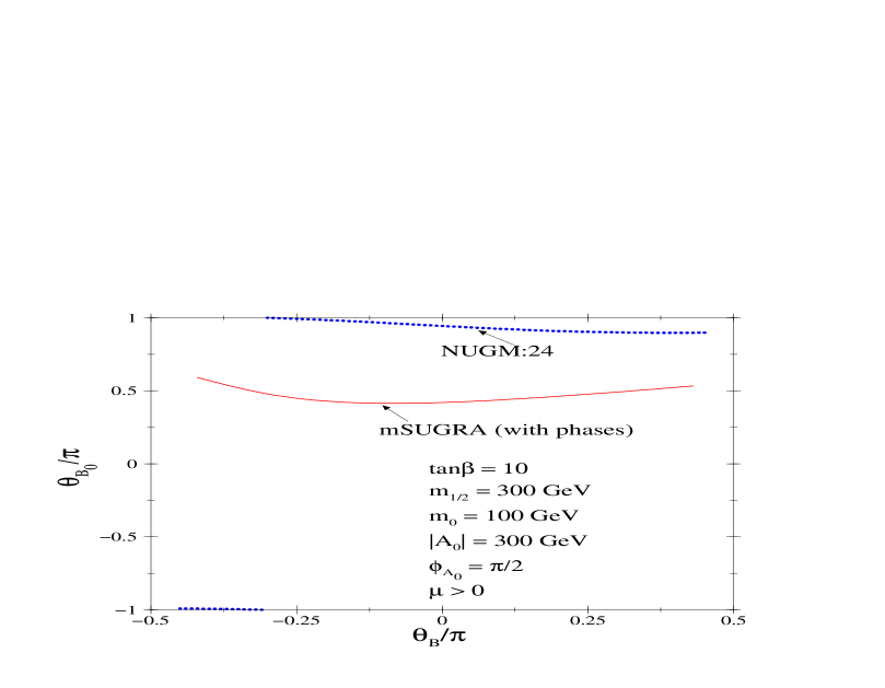
Figure 4: $\theta_{B_{0}}$ vs $\theta_{B}$ for $\tan\beta=3$ and 10 with other parameters are as shown for mSUGRA and NUGM:24 scenarios. $\theta_{B_{0}}$ (defined to lie in the range $[-\pi,\pi]$) is seen to be larger for NUGM:24.

Having established that the degree of fine tuning could, in principle, be smaller in the NUGM:24 case, we now perform a scan of the parameter space for both mSUGRA and NUGM:24 so as to quantify the extent of this reduction. In each case, we consider two different values of $\tan\beta$ ($=2,10$) while maintaining $\phi_{A_{0}}=\pi/2$ so as to maximize the EDM values. Allowing $m_{0}$, $m_{\frac{1}{2}}$ and $|A_{0}|$ to vary up to 1 TeV (with the lower end set in accordance with the current limits on super-particle masses), we show, in Figs.5, the scatter plots in the $\Phi$–$m_{\frac{1}{2}}$ plane. It is interesting to note that, for low to moderate values of $\tan\beta$, the measure $\Phi$ rarely becomes negative in the mSUGRA case, whereas in the non-universal scenario it is more evenly distributed.

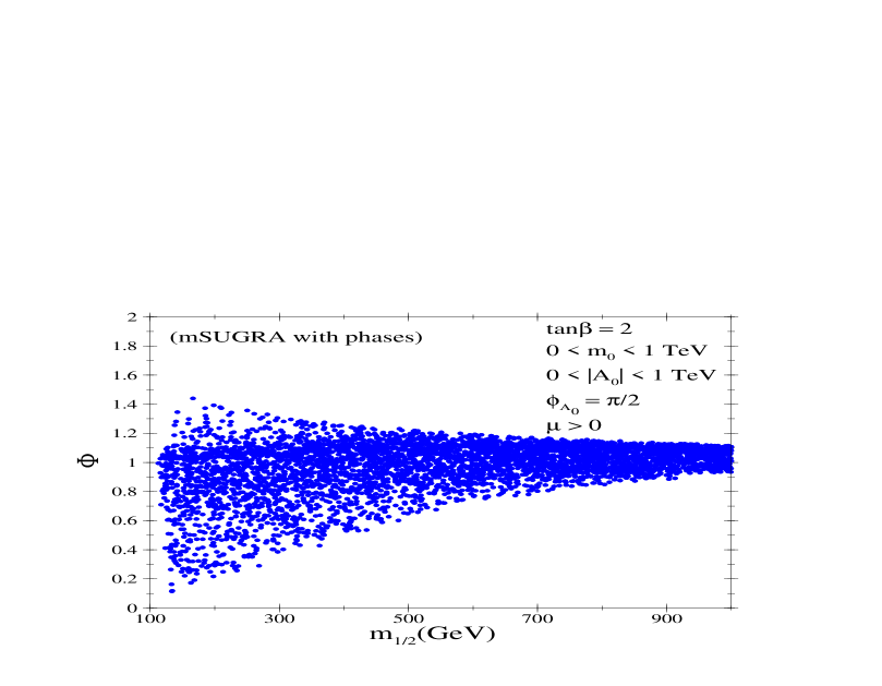
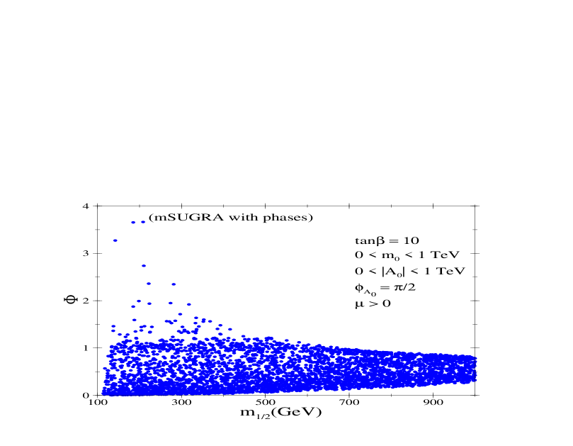
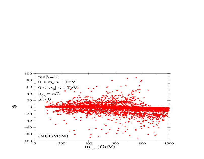
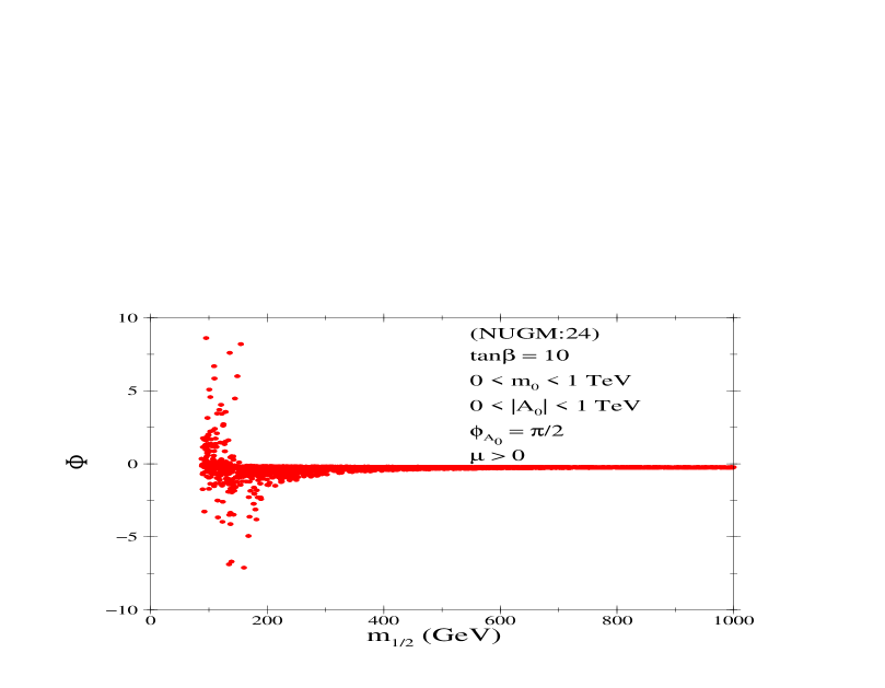
Figure 5: $\Phi$ vs $m_{\frac{1}{2}}$ for mSUGRA and NUGM:24 for $\tan\beta=2$ and $10$, when $m_{0}$ and $|A_{0}|$ are scanned up to 1 TeV for $\phi_{A_{0}}=\pi/2$.

While $|\Phi|$ does tend to concentrate around zero (Fig.5), note that, for small $\tan\beta$, the NUGM:24 case does have a significantly dense distribution up to $|\Phi|\sim 20$ and values as large as $|\Phi|\sim 100$ are also obtained, albeit with a reduced frequency. In contrast, the mSUGRA case barely registers a presence even for $\Phi\sim 1.5$ (Fig.5). Thus, in going from mSUGRA to NUGM:24, the fine-tuning can be reduced by a factor as large as $\sim 70$. For the $\tan\beta=10$ case though, the improvement is much more moderate. As Fig.5 shows, the mSUGRA scatter reaches up to $\Phi\sim 3.5$, whereas the non-universal scenario admits $|\Phi|\sim 10$ (Fig.5), or, in other words, a reduction of the maximal fine tuning by a factor of $\sim 3$. More important, though, is that the density of points at higher $\Phi$ is much larger in the NUGM:24 case than for mSUGRA. In other words, it is far more likely to have a less fine-tuned point in the parameter space for NUGM:24.

Concentrating on NUGM:24, we present, in Fig.6, contour plots for $\Phi$ in the $m_{0}-m_{\frac{1}{2}}$ plane for two different values of $\tan\beta$. Note that the limits on $m_{0}$ and $m_{\frac{1}{2}}$ are $2$ TeV, higher than what was chosen for Fig.5. Once again, $|A_{0}|$ is fixed at $100\rm~{}GeV$ with $\phi_{A_{0}}=\pi/2$. A comparison of the two plots clearly reinforces our earlier result that the fine-tuning is less severe for low $\tan\beta$. Furthermore, the values of $m_{0}$ and $m_{\frac{1}{2}}$ leading to a particular $\Phi$ are highly correlated. Note that both signs for $\Phi$ are possible. The region where $\Phi$ changes sign is associated with a parameter point where $\theta_{B_{0}}$ is $\sim\pi/2$. To summarize, the results displayed in Fig.5 and Fig.6 show that it is indeed possible to obtain a surprisingly large amount of reduction of phase sensitivity even for relatively small sparticle masses.

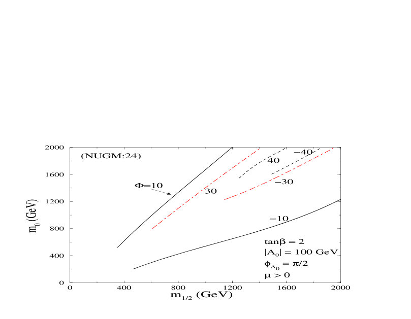
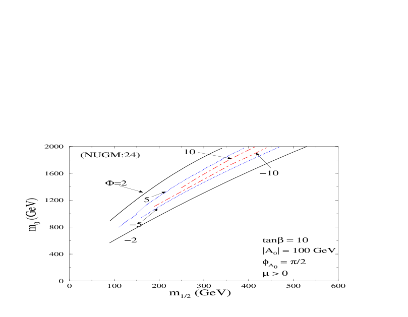
Figure 6: Contours of $\Phi$ in $m_{\frac{1}{2}}-m_{0}$ plane for $\tan\beta=2$ and $10$ in NUGM:24. A larger $|\Phi|$ corresponds to a lesser degree of phase sensitivity. Switching of the sign of $\Phi$ in some region of parameter space is associated with $\theta_{B_{0}}$ crossing $\pi/2$. Here $|A_{0}|=100\rm~{}GeV$ and $\phi_{A_{0}}=\pi/2$. Smaller $\tan\beta$ cases have larger values for $|\Phi|$.

We now explore, in detail, the range of $\tan\beta$ that is associated with very low level of phase sensitivity or, in other words, a very large $|\Phi|$. As has been argued earlier, $|B|$ itself strongly depends on $\tan\beta$. Moreover, $\Delta B$, and thereby $B_{0}$ too, has a nontrivial dependence on $\tan\beta$. Thus it is understandable that a very large $|\Phi|$ would indeed prominently highlight such a dependence. Rather than attempting a full, but very computing-intensive, scan over the entire parameter space, we choose to restrict ourselves to the subset of the parameter space that would naturally produce very large values for $|\Phi|$, namely the region with small $|B_{0}|$ and small $|A_{0}|$. Hence we adopt a framework with given values for $|B_{0}|$ instead of $\tan\beta$. The requirement of REWSB determines $\tan\beta$ once $B_{0}$, $m_{0}$, $m_{\frac{1}{2}}$ and $A_{0}$ are fixed. Note however, that the point $A_{0}=B_{0}=0$ would imply the absence of any SUSY CP phase at all scales. Thus, it is not surprising to obtain very large values of $|\Phi|$ in this scenario. However, in this part of our work the focus is simply to study, the effect of $\tan\beta$ on $\Phi$ in detail, more importantly for large $|\Phi|$ values. To quantify our study of this issue, we choose small representative values viz. $|B_{0}|=0.5\rm~{}GeV$ and $|A_{0}|=1\rm~{}GeV$, along with $\phi_{A_{0}}=\pi/2$ so as to maximize the EDM contributions as before. In Figs.7, we present various scatter plots for $\Phi$ as $m_{0}$ and $m_{\frac{1}{2}}$ are varied over a wide range (0 to 2 TeV). Note that the results of this analysis have a significant dependence on $|A_{0}|$. For example, increasing $|A_{0}|$ to $100$ GeV may reduce $\Phi$ by a factor of 10 to 20. As Fig.7 shows, within mSUGRA, $|\Phi|$ could be as large as $100$ while most of the points lie between $10$ to $25$. The situation is qualitatively different in NUGM:24 (Fig.7) where $|\Phi|$ may go up to $1500$ while typically ranging between $200$ to $600$. Thus, NUGM:24 is much better able to accommodate low phase-sensitivity solutions than do the universal gaugino mass scenarios.

It is curious to note that, unlike what Fig.5 suggested, $\Phi$ could assume negative values within mSUGRA (see Fig.7). This prompts us present a scatter plot of $\Phi$ against the derived quantity $\tan\beta$. As Fig.7 shows, mSUGRA admits negative $\Phi$ only for large $\tan\beta$. In fact, even for the positive branch, large values of $|\Phi|$ are typically concentrated in the large $\tan\beta$ (20 to 45) region. In contrast, for NUGM:24, $\Phi$ assumes larger values typically for low $\tan\beta$ values (2 to 5). It should be remembered in this context that, within NUGM:24, the large $\tan\beta$ domain is significantly restricted from considerations of the LSP (see Sec.3.1). That the favored range for $\tan\beta$ is different in the two scenarios is attributable to the interplay between the cancellations/enhancements in the RGE evolution of $B$ on the one hand and the requirement of REWSB on the other.

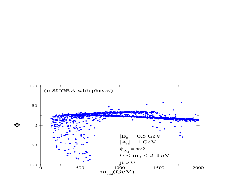
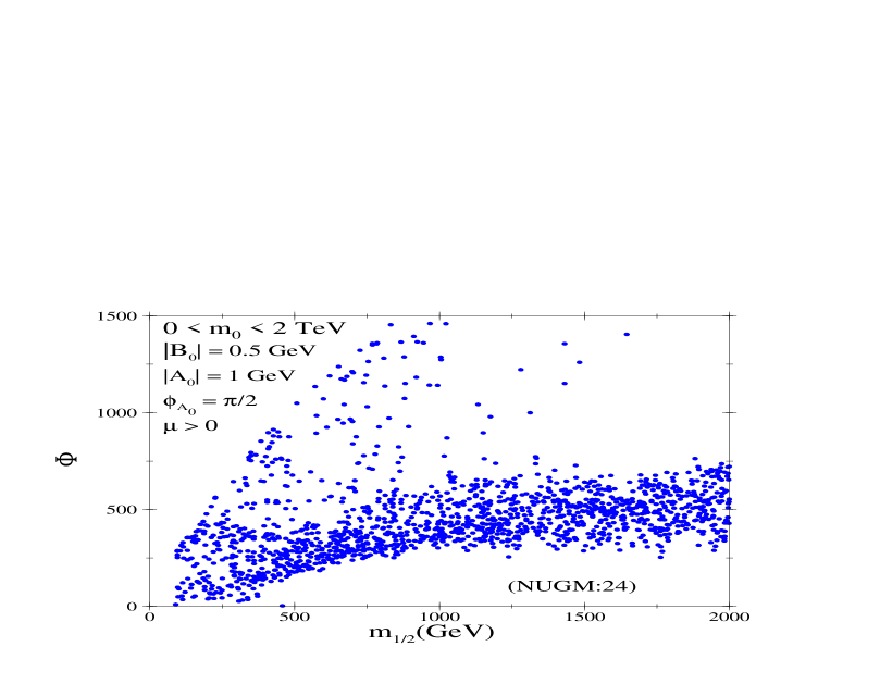
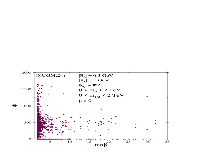
Figure 7: a) and b): Scatter plots corresponding to large values of $|\Phi|$ for mSUGRA and NUGM:24 cases. A smaller value for $|B_{0}|$ as well as smaller $|A_{0}|$ enhance $|\Phi|$ both in mSUGRA and NUGM:24. However, NUGM:24 is associated with much larger values for $|\Phi|$ as compared to mSUGRA. c) and d): Displays of the associated values of $\tan\beta$ vs $\Phi$. $\tan\beta$ is small (2 to 5) for NUGM:24, whereas the same for mSUGRA is large (20 to 45).

Finally, we comment on the case of $\mu<0$. It turns out that for this branch of $\mu$ and $\phi_{A_{0}}=\pi/2$, one has $|B_{0}|>|B|$ for almost all the parameter space of NUGM:24. As a result one finds no advantage toward reducing the phase sensitivity.

4 Conclusion

As is well known, the experimental upper bounds on the electric dipole moments of the neutron and the electron impose strong constraints on any source of $CP$ violation in supersymmetric models, in particular on the weak scale phase parameters. For example, in the minimal supergravity model, $\theta_{B}$, the phase of the bilinear Higgs coupling parameter is constrained to be typically smaller than $0.01$, with only some very limited regions (such as the focus point scenario) in the parameter space admitting slightly larger ($\mathrel{\mathchoice{\vbox{\offinterlineskip\halign{$\m@th\displaystyle\hfil#\hfil$\cr<\crcr\sim\crcr} }}{\vbox{\offinterlineskip\halign{$\m@th\textstyle\hfil#\hfil$\cr<\crcr\sim\crcr} }}{\vbox{\offinterlineskip\halign{$\m@th\scriptstyle\hfil#\hfil$\cr<\crcr\sim\crcr} }}{\vbox{\offinterlineskip\halign{$\m@th\scriptscriptstyle\hfil#\hfil$\cr<\crcr\sim\crcr} }}}0.1$) values. This, however, implies a severe fine-tuning condition for $\theta_{B_{0}}$, the value of the same phase parameter at the unification scale. In turn, $\phi_{A_{0}}$, the phase of the trilinear coupling parameter is also severely fine-tuned. This has been a longstanding problem with mSUGRA-like scenarios.

To quantify this problem, we define a phase naturalness measure $\Phi$ as the ratio of the spread of the phase $\theta_{B_{0}}$ at the unification scale that is consonant with the spread $\theta_{B}$ allowed, at the electroweak scale, by the electric dipole moment constraints A larger $\Phi$ would imply a lower degree of phase sensitivity. One finds that, unless $\tan\beta$ is very large, $\Phi$ may be approximated to $B/B_{0}$ for much of the parameter space.

In this analysis, we have demonstrated that models admitting a large RG evolution of the bilinear Higgs coupling could be interesting in the context of a reduction in the fine-tuning of phases. In particular, we choose a supergravity-inspired scenario wherein non-universal gaugino masses arise from a gauge kinetic energy function $f_{\alpha\beta}$ transforming as a particular non-singlet representation of $SU(5)$ (NUGM:24 of Table 1). As in the mSUGRA (singlet $f_{\alpha\beta}$) case, this representation, considered in isolation, introduces no additional phase for the gaugino masses.

Studying the nature of the evolution of $B$ to understand the correspondence with phase-sensitivity, we identify the large cancellations in the RGE for $B$ as being primarily responsible for the high degree of fine-tuning within mSUGRA. In the NUGM:24, on the other hand, the said cancellations are replaced by enhancements (on account of the reversal in the sign of the gaugino mass terms) and this translates into a reduction of the above-mentioned fine-tuning. In fact, $\Phi$ can be significantly increased in NUGM:24 (by a factor of 10 to 20) with respect to comparable mSUGRA type of models. The said improvement is typically more pronounced for small $\tan\beta$ values.

A particularly interesting result is the identification of extended regions in the NUGM:24 parameter space which admit a low degree of phase-sensitivity even for relatively small super-particle masses. This feature is absent in mSUGRA as well as in most other models with high scale inputs for SUSY breaking.

We further explored the dependence of our results, on $\tan\beta$, by specifically concentrating on the parameter space corresponding to very large $\Phi$ (or very small phase sensitivity) so as to compare the two models. Naturally, this occurs close to vanishing $A_{0}$ and $B_{0}$ values. We adopt a scheme where $B_{0}$ itself is given as an input parameter instead of $\tan\beta$, given the more direct relationship of $B_{0}$ with $\Phi$. Our analysis shows that, even here, the values of $\Phi$ in NUGM:24 are typically larger by a factor of 10 to 20 in comparison to those in mSUGRA. And whereas mSUGRA generically requires large $\tan\beta$ (20 to 40) for $|\Phi|$ to be large, the NUGM:24 scenario prefers a smaller $\tan\beta$ (2 to 5) instead.

Finally, while our analysis has focussed on $SU(5)$ as the GUT gauge group, similar considerations hold for $SO(10)$ as well. A suitable non-singlet representation resulting in a similar gaugino-mass pattern as in NUGM:24 would also produce such a reduction of phase sensitivity.

Acknowledgments
DC acknowledges financial assistance from the Department of Science and Technology, India under the Swarnajayanti Fellowship grant. DD would like to thank the Council of Scientific and Industrial Research, Govt. of India for the support received as a Junior Research Fellow.

References

- [1] See for example textbooks like: “Supersymmetry and Supergravity” by J. Wess and J. Bagger, Princeton Univ. Press, 1992 ; “Introduction To Supersymmetry And Supergravity” by P. C. West, World Scientific, Singapore, 1990; J. D. Lykken, arXiv:hep-th/9612114; “Theory and phenomenology of sparticles: An account of four-dimensional N=1 supersymmetry in high energy physics”, M. Drees, R. Godbole and P. Roy, World Scientific, Singapore, 2004.
- [2] See reviews like: H. E. Haber and G. L. Kane, Phys. Rept. 117, 75 (1985); S. P. Martin, arXiv:hep-ph/9709356.
- [3] D. J. H. Chung, L. L. Everett, G. L. Kane, S. F. King, J. Lykken and L. T. Wang, arXiv:hep-ph/0312378.
- [4] A. H. Chamseddine, R. Arnowitt and P. Nath, Phys. Rev. Lett. 49, 970 (1982).
- [5] For reviews see P. Nath, R. Arnowitt and A.H. Chamseddine, Applied N =1 Supergravity (World Scientific, Singapore, 1984); H.P. Nilles, Phys. Rep. 110, 1 (1984); R. Arnowitt and P. Nath, Proc. of VII J.A. Swieca Summer School ed. E. Eboli (World Scientific, Singapore, 1994).
- [6] E. Cremmer, S. Ferrara, L. Girardello and A. van Proeyen, Phys. Lett. 116B, 231 (1982); Nucl. Phys. B212, 413 (1983); E. Witten and J. Bagger, Nucl. Phys. B222,1 (1983).
- [7] P. Nath, R. Arnowitt and A. H. Chamseddine, Nucl. Phys. B 227, 121 (1983).
- [8] L. J. Hall, J. Lykken and S. Weinberg, Phys. Rev. D 27, 2359 (1983); N. Ohta, Prog. Theor. Phys. 70, 542 (1983).
- [9] L.E. Ibañez, Phys. Lett. B118, 73 (1982); P. Nath, R. Arnowitt and A. H. Chamseddine, Phys. Lett. B 121, 33 (1983); R. Arnowitt, A. H. Chamseddine and P. Nath, Phys. Lett. B 120, 145 (1983); J. Ellis, D. V. Nanopoulos and K. Tamvakis, Phys. Lett. B121, 123 (1983).
- [10] K. Inoue et al., Prog. Theor. Phys. 68, 927 (1982); L. Ibañez and G. G. Ross, Phys. Lett. B110, 215 (1982); L. Alvarez-Gaumé, J. Polchinski and M. B. Wise, Nucl. Phys. B221, 495 (1983); J. Ellis, J. Hagelin, D. V. Nanopoulos and K. Tamvakis, Phys. Lett. B125, 275 (1983); L. E. Ibañez and C. Lopez, Phys. Lett. B126, 54 (1983); Nucl. Phys. B233, 511 (1984); L. E. Ibañez, C. Lopez and C. Muños, Nucl. Phys. B256, 218 (1985); J. Ellis and F. Zwirner, Nucl. Phys. B338, 317 (1990).
- [11] M. E. Machacek and M. T. Vaughn, Nucl. Phys. B 222, 83 (1983); Nucl. Phys. B 236, 221 (1984); Nucl. Phys. B 249, 70 (1985).
- [12] S. P. Martin and M. T. Vaughn, Phys. Lett. B 318, 331 (1993) [arXiv:hep-ph/9308222]; Phys. Rev. D 50, 2282 (1994) [arXiv:hep-ph/9311340]; I. Jack, D. R. Jones, S. P. Martin, M. T. Vaughn and Y. Yamada, Phys. Rev. D 50, R5481 (1994) [arXiv:hep-ph/9407291].
- [13] S. Abel et al. [SUGRA Working Group Collaboration], arXiv:hep-ph/0003154.
- [14] T. Ibrahim and P. Nath, Phys. Rev. D 58, 111301 (1998), [Erratum-ibid. D 60, 099902 (1999)] [arXiv:hep-ph/9807501]; M. Brhlik, G. J. Good and G. L. Kane, Phys. Rev. D 59, 115004 (1999) [arXiv:hep-ph/9810457].
- [15] E. Accomando, R. Arnowitt and B. Dutta, Phys. Rev. D 61, 115003 (2000) [arXiv:hep-ph/9907446].
- [16] R. Arnowitt, B. Dutta and Y. Santoso, Phys. Rev. D 64, 113010 (2001) [arXiv:hep-ph/0106089].
- [17] E. Accomando, R. Arnowitt and B. Dutta, Phys. Rev. D 61, 075010 (2000) [arXiv:hep-ph/9909333].
- [18] V. D. Barger, T. Falk, T. Han, J. Jiang, T. Li and T. Plehn, Phys. Rev. D 64, 056007 (2001) [arXiv:hep-ph/0101106].
- [19] T. Falk and K. A. Olive, Phys. Lett. B 439, 71 (1998) [arXiv:hep-ph/9806236].
- [20] R. Garisto and J. D. Wells, Phys. Rev. D 55, 1611 (1997) [arXiv:hep-ph/9609511].
- [21] T. Ibrahim and P. Nath, Phys. Rev. D 61, 093004 (2000) [arXiv:hep-ph/9910553]; M. Brhlik, G. J. Good and G. L. Kane, Phys. Rev. D 59, 115004 (1999) [arXiv:hep-ph/9810457]; T. Ibrahim and P. Nath, Phys. Rev. D 57, 478 (1998) [Erratum-ibid. D 58, 019901 (1998 ERRAT,D60,079903.1999 ERRAT,D60,119901.1999)] [arXiv:hep-ph/9708456].
- [22] A. Bartl, W. Majerotto, W. Porod and D. Wyler, Phys. Rev. D 68, 053005 (2003) [arXiv:hep-ph/0306050]; S. Abel, S. Khalil and O. Lebedev, Nucl. Phys. B 606, 151 (2001) [arXiv:hep-ph/0103320]; A. Bartl, T. Gajdosik, W. Porod, P. Stockinger and H. Stremnitzer, Phys. Rev. D 60, 073003 (1999) [arXiv:hep-ph/9903402]; D. Chang, W. Y. Keung and A. Pilaftsis, Phys. Rev. Lett. 82, 900 (1999) [Erratum-ibid. 83, 3972 (1999)] [arXiv:hep-ph/9811202]
- [23] U. Chattopadhyay, T. Ibrahim and D. P. Roy, Phys. Rev. D 64, 013004 (2001) [arXiv:hep-ph/0012337]; J. L. Feng and K. T. Matchev, Phys. Rev. D 63, 095003 (2001) [arXiv:hep-ph/0011356].
- [24] J. Ellis,K. Enqvist,D. V. Nanopoulos, and K. Tamvakis, Phys. Lett. 155B, 381(1985); M. Drees, Phys. Lett. B158,409(1985); K. Huitu, Y. Kawamura, T. Kobayashi and K. Puolamaki, Phys. Rev. D 61, 035001 (2000).
- [25] A. Corsetti and P. Nath, Phys. Rev. D 64, 125010 (2001); hep-ph/0005234; hep-ph/0011313.
- [26] C. T. Hill, Phys. Lett. B 135, 47 (1984); Q. Shafi and C. Wetterich, Phys. Rev. Lett. 52, 875 (1984); T. Dasgupta, P. Mamales and P. Nath, Phys. Rev. D 52, 5366 (1995).
- [27] G. Anderson, C.H. Chen, J.F. Gunion, J. Lykken, T. Moroi, and Y. Yamada, hep-ph/9609457; G. Anderson, H. Baer, C-H Chen and X. Tata, Phys. Rev. D 61, 095005 (2000).
- [28] K. Huitu, J. Laamanen, P. N. Pandita and S. Roy, arXiv:hep-ph/0502100; U. Chattopadhyay and D. P. Roy, Phys. Rev. D 68, 033010 (2003) [arXiv:hep-ph/0304108]; U. Chattopadhyay and P. Nath, Phys. Rev. D 65, 075009 (2002) [arXiv:hep-ph/0110341].
- [29] U. Chattopadhyay, A. Corsetti and P. Nath, Phys. Rev. D 66, 035003 (2002) [arXiv:hep-ph/0201001].
- [30] N. Chamoun, C-S Huang, C Liu, and X-H Wu, Nucl. Phys. B624, 81 (2002). [arXiv:hep-ph/0110332].
- [31] J. R. Ellis, C. Kounnas and D. V. Nanopoulos, Nucl. Phys. B 247, 373 (1984). See also Chattopadhyay and Nath of Ref.[28].
- [32] R. Arnowitt and P. Nath, Phys. Rev. D 46, 3981 (1992).
- [33] G. Gamberini, G. Ridolfi and F. Zwirner, Nucl. Phys. B 331, 331 (1990); V. D. Barger, M. S. Berger and P. Ohmann, Phys. Rev. D 49, 4908 (1994); For two-loop effective potential see: S. P. Martin, Phys. Rev. D 66, 096001 (2002).
- [34] K. L. Chan, U. Chattopadhyay and P. Nath, Phys. Rev. D 58, 096004 (1998) [arXiv:hep-ph/9710473].
- [35] U. Chattopadhyay, A. Corsetti and P. Nath, Phys. Rev. D 68, 035005 (2003); J. L. Feng, K. T. Matchev and T. Moroi, Phys. Rev. D 61, 075005 (2000).