Renormalization of the EWCL and its Application to LEP2

Abstract

We perform a systematic one-loop renormalization on the electroweak chiral Lagrangian (EWCL) up to $O(p^{4})$ operators and construct the renormalization group equations (RGE) for the anomalous couplings. We examine the impact of the triple gauge coupling (TGC) measurement from LEP2 to the uncertainty of the $S-T$ parameter at the $\Lambda=1TeV$, and find that the uncertainty in the TGC measurements can shift $S(\Lambda)$ at least $3.3\sigma$.

TKYNT-05/21

1 Introduction

Direct precision measurement on the TGC at LEP2 reinforces [1, 2, 3, 4, 5, 6] our belief that the standard model is the correct description for the particle physics phenomenology. However, Higgs is still an elusive particle and the electroweak symmetry breaking mechanism is still a mystery. Therefore, it is reasonable and necessary to interpret the Z pole data and LEP2 TGC data in a model independent fashion without a Higgs boson, so as to give some guides to model-building works. Such an effective description is given as the EWCL [7, 8, 9], where the Goldstone particles are parameterized in nonlinear form.

In order to extrapolate electroweak precision data collected at low energy region $\mu=m_{\textrm{Z}}$ up to the ultraviolet cutoff $\Lambda=1TeV$, radiative corrections of the EWCL must be correctly and efficiently summed over. There are several groups who have considered the radiative corrections within the EWCL by including anomalous couplings, due to different assumptions and technique uncertainties, those results do not agree with each other [10, 11, 12, 13, 14, 15]. For example, the $\beta$ function of anomalous couplings in the unitary gauge with dimensional regularization [13, 14] do not agree with well-known results [8]. It seems a puzzle whether the radiative corrections in the EWCL with dimensionless anomalous couplings is well-defined or not [10].

Therefore our project is to perform such a systematic renormalization for the EWCL to investigate this puzzle. We use the background field method, a renormalizable gauge, path integral, dimensional and heat kernel regularization, ${\overline{MS}}$ renormalization scheme [16], to perform the systematic one-loop expansion to the EWCL and construct the RGE of those dimensionless anomalous couplings. There are some preliminary results [17], and now they are almost finished [18].

We use our RGE method to analyze the electroweak precision data at Z poles and TGC.

2 The renormalization group equations

We construct the counter terms for all $O(p^{2})$ and $O(p^{4})$ operators at one loop level and succeed in building the RGE. Our power counting rule in loop expansion is equivalent to the large $N$ and standard mass dimension power counting rules. In the realistic analysis, we can keep only linear terms of anomalous couplings in the $\beta$ function [19]. By assuming that ghosts are complex ghosts, we handle the nonhermitean ghost term in a simple way. Then, the $\beta$ functions of two point parameters are given as:

$$\beta_{{\alpha}_{1}} = \frac{1}{12}+2{\alpha}_{1}g^{2}+{\alpha}_{8}g^{2}+\frac{5{\alpha}_{2}g^{2}}{2}-\frac{5{\alpha}_{3}g^{2}}{6}+\frac{{\alpha}_{9}g^{2}}{2}\,,$$ (1)

$$\beta_{{\alpha}_{8}} = {\beta\over 2}-{\alpha}_{1}{g^{\prime}}^{2}+\frac{37{\alpha}_{8}g^{2}}{6}+\frac{5{\alpha}_{2}{g^{\prime}}^{2}}{6}-\frac{{\alpha}_{3}{g^{\prime}}^{2}}{2}+\frac{17{\alpha}_{9}g^{2}}{6}\,,$$ (2)

$$\beta_{\beta} = -\frac{3{g^{\prime}}^{2}}{8}-{15\beta g^{2}\over 4}-{3\beta{g^{\prime}}^{2}\over 4}+{\alpha}_{1}\bigg{(}\frac{9g^{2}{g^{\prime}}^{2}}{4}+\frac{{g^{\prime}}^{4}g^{2}}{2G^{2}}\bigg{)}+{\alpha}_{8}\bigg{(}\frac{g^{4}}{8}-\frac{{g^{\prime}}^{2}g^{4}}{4G^{2}}\bigg{)}$$ (3)

$$+{\alpha}_{2}\bigg{(}\frac{5g^{2}{g^{\prime}}^{2}}{2}-\frac{3{g^{\prime}}^{4}}{4}\bigg{)}+{\alpha}_{3}\frac{5g^{2}{g^{\prime}}^{2}}{2}+{\alpha}_{9}\bigg{(}-\frac{g^{4}}{2}+\frac{3g^{2}{g^{\prime}}^{2}}{4}\bigg{)}$$

$$-{\alpha}_{4}\bigg{(}\frac{15g^{2}{g^{\prime}}^{2}}{4}+\frac{15{g^{\prime}}^{4}}{8}\bigg{)}-{\alpha}_{5}\bigg{(}\frac{3g^{2}{g^{\prime}}^{2}}{2}+\frac{3{g^{\prime}}^{4}}{4}\bigg{)}$$

$$-{\alpha}_{6}\bigg{(}\frac{3g^{4}}{4}+\frac{33G^{4}}{8}\bigg{)}-{\alpha}_{7}\bigg{(}3g^{4}+3G^{4}\bigg{)}-{\alpha}_{10}\bigg{(}\frac{9G^{4}}{2}\bigg{)}\,.$$

Here we have organized these $\beta$ functions in the order of the contributions from the constant terms and the quadratic, triple, and quadruple anomalous couplings.

We omitted other $\beta$ functions here due to the reason that they are not directly related with $S-T$ fitting.

3 Application to precision data

In order to be as general as possible, we have not imposed the custodial symmetry in our analysis.

Although D0 collaboration at Tevatron [6] has reported their measurements on the TGC, errors are much larger than those at LEP2. Therefore we use the data published by the L3 collaboration and the combined fit results from LEP EW working group [5] in our analysis.

We have taken $\delta k_{Z}=-.076\pm 0.064$ from L3 [3], and $\delta k_{\gamma}=-.027\pm 0.045$ and $\delta g_{Z}^{1}=-0.016\pm 0.022$ from [5] as inputs to determine the anomalous couplings ${\alpha}_{2}$, ${\alpha}_{3}$, and ${\alpha}_{9}$. These data are extracted from one-parameter TGC fits and the last two are extracted by imposing the custodial symmetry. Each of data corresponds to a set of solution for ${\alpha}_{2}$ , ${\alpha}_{3}$, and ${\alpha}_{9}$. In order to combine these data in our analysis, we assume that these data are extracted from independent measurements (From the theoretical viewpoint, these measurements must be correlated but the the correlation is energy-dependent).

With the above assumption, we find

$$\begin{array}[]{rl}{\alpha}_{2}=\!\!\!&(-0.09\pm 0.14)\\ {\alpha}_{3}=\!\!\!&(-0.03\pm 0.04)\\ {\alpha}_{9}=\!\!\!&(0.12\pm 0.12)\end{array}\rho_{corr.}=\left(\begin{matrix}1\,\,\,&&\cr 0&1\,\,\,&\cr-.68&-.32&1\,\,\,\cr\end{matrix}\right).$$ (4)

The $S(\Lambda)$ and $T(\Lambda)$ are depicted in Fig. 1. The solid curves correspond to the analysis including the contributions of the TGC, while the dashed curves correspond to the analysis discarding the contributions of the TGC. The effects of ultraviolet cutoff are shown by taking three values of ultraviolet cutoff $\Lambda=$ $300$ GeV, $1$ TeV, and $3$ TeV, respectively. The $S-T$ contour at $\mu=m_{\textrm{Z}}$ is depicted as a reference contour to compare.

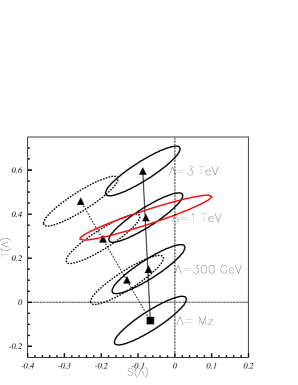
Figure 1: $S(\Lambda)-T(\Lambda)$ contours at $\Lambda=m_{\textrm{Z}}$, $300$ GeV, $1$ TeV, and $3$ TeV, respectively. Solid curves have incorporated the contributions of the TGC, while the dashed curves haven’t.

Without including the contribution of the TGC, $S(\Lambda)$ goes to the negative value direction with the increase of $\Lambda$ in agreement with the observation of Ref. [20]. However, when taking into account the contributions of the TGC with the central value of LEP2 fit in Eq. (4), we observe that the allowed region of $S(\Lambda)$ and $T(\Lambda)$ shifts toward positive $S(\Lambda)$ and positive $T(\Lambda)$.

The contour generated by including $1\,\sigma$ errors of ${\alpha}_{2}-{\alpha}_{3}-{\alpha}_{9}$ (the largest contour in Fig. 1 at $\Lambda=1$ TeV) shows that $S(\Lambda)$ can vary from $-0.26$ to $0.1$. We observe that the uncertainty in the anomalous TGC can swing the central value of $S(\Lambda)$ at least $3.3\sigma$ away.

4 Conclusion

We have performed the one-loop systematic renormalization on the EWCL. Our results agree with well-known results [8] if anomalous couplings vanish (sign differences are due to the Euclidean space convention and the definition of covariant differential operator). Our results show that in the EWCL those dimensionless anomalous couplings run in a logarithmic way. However, there is still one puzzle left: what’s the meaning of nonhermitean ghost term? What’s the correct method to treat it?

We have analyzed the uncertainty of $S(\Lambda)$ caused by the uncertainty of TGC measurements, which can swing the $S(\Lambda)$ at least $3.3\sigma$ away.

References

- [1] A. Heister et al. [ALEPH Collaboration], Eur. Phys. J. C 21, 423 (2001).
- [2] G. Abbiendi et al. [OPAL Collaboration], Eur. Phys. J. C 33, 463 (2004).
- [3] P. Achard et al. [L3 Collaboration], Phys. Lett. B 586, 151 (2004).
- [4] S. Schael et al. [ALEPH Collaboration], Phys. Lett. B 614, 7 (2005).
- [5] LEPEWWG/TGC/2005-01, http://www.cern.ch/LEPEWWG/lepww/tgc.
- [6] V. M. Abazov et al. [D0 Collaboration], arXiv:hep-ex/0504019.
- [7] T. Appelquist and C. W. Bernard, Phys. Rev. D 22, 200 (1980); Phys. Rev. D 23, 425 (1981).
- [8] A. C. Longhitano, Phys. Rev. D 22, 1166 (1980); Nucl. Phys. B 188, 118 (1981).
- [9] T. Appelquist and G. H. Wu, Phys. Rev. D 48, 3235 (1993) [arXiv:hep-ph/9304240].
- [10] A. De Rujula, M. B. Gavela, P. Hernandez and E. Masso, Nucl. Phys. B 384, 3 (1992).
- [11] K. Hagiwara, S. Ishihara, R. Szalapski and D. Zeppenfeld, Phys. Lett. B 283, 353 (1992); Phys. Rev. D 48, 2182 (1993).
- [12] P. Hernandez and F. J. Vegas, Phys. Lett. B 307, 116 (1993) [arXiv:hep-ph/9212229].
- [13] C. P. Burgess, S. Godfrey, H. Konig, D. London and I. Maksymyk, Phys. Rev. D 50 (1994) 7011 [arXiv:hep-ph/9307223].
- [14] S. Dawson and G. Valencia, Nucl. Phys. B 439, 3 (1995) [arXiv:hep-ph/9410364].
- [15] J. J. van der Bij and B. M. Kastening, Phys. Rev. D 57, 2903 (1998).
- [16] Q. S. Yan and D. S. Du, Phys. Rev. D 69, 085006 (2004); S. Dutta, K. Hagiwara and Q. S. Yan, Nucl. Phys. B 704, 75 (2005).
- [17] Qi-Shu Yan, hep-ph/0409150; Qi-Shu Yan and Dong-Sheng Du, published in APPI 2003, Accelerator and Particle Pyysics, 108; Qi-Shu Yan and Dong-Sheng Du, hep-ph/0212367.
- [18] S. Dutta, K. Hagiwara and Q. S. Yan, in preparation.
- [19] H. Georgi, Phys. Lett. B 298 (1993) 187; H. J. He, Y. P. Kuang and C. P. Yuan, Phys. Lett. B 382, 149 (1996).
- [20] J. A. Bagger et. al. , Phys. Rev. Lett. 84, 1385 (2000); M. E. Peskin and J. D. Wells, Phys. Rev. D 64, 093003 (2001).