Abstract

Starting from a (new physics independent) tree level determination of $\bar{\rho}$ and $\bar{\eta}$, we perform the Unitarity Triangle analysis in general extensions of the Standard Model with arbitrary new physics contributions to loop-mediated processes. Using a simple parameterization, we determine the allowed ranges of non-standard contributions to $|\Delta F|=2$ processes. Remarkably, the recent measurements from $B$ factories allow us to determine with good precision the shape of the Unitarity Triangle even in the presence of new physics, and to derive stringent constraints on non-standard contributions to $|\Delta F|=2$ processes. Since the present experimental constraints favour models with Minimal Flavour Violation, we present the determination of the Universal Unitarity Triangle that can be defined in this class of extensions of the Standard Model. Finally, we perform a combined fit of the Unitarity Triangle and of new physics contributions in Minimal Flavour Violation, reaching a sensitivity to a new physics scale of about 5 TeV. We also extrapolate all these analyses into a “year 2010” scenario for experimental and theoretical inputs in the flavour sector. All the results presented in this paper are also available at the URL http://www.utfit.org, where they are continuously updated.

1 Introduction

With the increasing precision of the experimental results, the Unitarity Triangle (UT) analysis shows the impressive success of the CKM picture in describing CP violation in the Standard Model (SM). UT parameters have been consistently determined using both CP-conserving ($|V_{ub}/V_{cb}|$, $\Delta m_{d}$ and ${\Delta m_{d}}/{\Delta m_{s}}$) and CP-violating ($\varepsilon_{K}$ and $\sin 2\beta$) processes [1]. Additional measurements of several combinations of angles of the UT, especially $\gamma$ from $B\to DK$ and $\alpha$ from charmless $B$ decays, confirm this picture [1].

This success becomes a puzzle once, as a possible solution to the gauge hierarchy problem, the SM is considered as an effective theory valid up to energies not much higher than the electroweak scale. Indeed, even in the favourable case in which the theory above the cutoff is weakly coupled, such as the Minimal Supersymmetric Standard Model, large contributions to Flavour Changing Neutral Current (FCNC) and CP-violating processes are expected to arise [2], clashing with the large amount of accurate experimental data now available on these transitions. This is due to the presence of additional sources of flavour and CP violation beyond the CKM matrix (see for example Ref. [3] for the supersymmetry case).

In general, the flavour puzzle admits two classes of possible solutions. The first one contains models in which a flavour symmetry is invoked to explain the hierarchy of quark masses and mixing angles. These models are based on different theoretical approaches (supersymmetry, grand unification, extra dimensions, …) leading to different levels of agreement with the data and to different low-energy signals. However, low-energy processes generally receive sizable additional contributions which jeopardize the validity of the SM UT analysis (see Ref. [4] for a supersymmetric example). A generalized UT fit allowing for the presence of arbitrary New Physics (NP) contributions is therefore very useful for model building, since it provides at the same time the allowed ranges for the SM CKM parameters and for the NP contributions to $|\Delta F|=2$ processes. This will be the subject of the first part of the present work (Secs. 2-4).

The second class of solutions to the flavour puzzle contains models with Minimal Flavour Violation (MFV). The basic idea of MFV is that the only source of flavour violation is in the SM Yukawa couplings, so that all FCNC and CP-violating phenomena can be expressed in terms of the CKM matrix and the top quark Yukawa coupling [5, 6, 7]. This leads to strong correlations between different observables, and allows for a detailed study of low-energy phenomena. While there are several implementations of MFV in different contexts (two-Higgs doublet models, supersymmetry [8], extra dimensions [9], …), it is possible to perform two very general analyses under the MFV hypothesis. The first is the determination of the so-called Universal Unitarity Triangle (UUT) [5], which is a UT fit performed using only quantities that are independent of NP contributions within MFV models. The second is a simultaneous fit of the UT and of NP contributions in the $|\Delta F|=2$ sector. These two analyses will be presented in the second part of this work (Sec. 5), and they serve as the starting point for the study of rare decays and CP violation in MFV models [10].

Finally, in Sec. 6 we present the possible future improvements in the above analyses by considering a “year 2010” scenario for experimental data and theoretical inputs in the flavour sector.

While to our knowledge the determination of the UUT is presented in this work for the first time, several attempts have been previously made in the study of the UT in the presence of NP. Considering only model-independent analyses, in Ref. [11] the case of NP contributions to $|\Delta B|=2$ or $|\Delta S|=2$ transitions was analyzed: this corresponds to the discussion in Section 4 of the present work. A first version of the present analysis, with some experimental constraints missing, was presented in Ref. [12]. Constraints on NP in the $|\Delta B|=2$ sector using $B$ physics only were considered in Refs. [13, 14, 15]. The determination of the UT from tree-level processes only was presented in Ref. [1]. A general analysis was recently performed in Ref. [16], but not all available constraints were used. With respect to these previous studies, we improve several theoretical aspects and perform a simultaneous determination of UT and NP parameters using all the available constraints in all sectors.

A compilation of the experimental and theoretical inputs to our analyses is presented in Table 1.

Parameter	Value	Gaussian ($\sigma$)	Uniform
			(half-width)
$\lambda$	0.2258	0.0014	-
$\left|V_{cb}\right|$(excl.)	$41.3\times 10^{-3}$	$1.0\times 10^{-3}$	$1.8\times 10^{-3}$
$\left|V_{cb}\right|$(incl.)	$41.6\times 10^{-3}$	$0.7\times 10^{-3}$	-
$\left|V_{ub}\right|$(excl.)	$38.0\times 10^{-4}$	$2.7\times 10^{-4}$	$4.7\times 10^{-4}$
$\left|V_{ub}\right|$(incl.)	$43.9\times 10^{-4}$	$2.0\times 10^{-4}$	$2.7\times 10^{-4}$
$\Delta m_{d}$ [ps-1]	$0.501$	$0.005$	-
$\Delta m_{s}$ [ps-1]	$>$ 14.5 at 95% C.L.	sensitivity 18.3
$F_{B_{s}}\sqrt{\hat{B}_{B_{s}}}$ [MeV]	$276$	$38$	-
$\xi=\frac{F_{B_{s}}\sqrt{\hat{B}_{B_{s}}}}{F_{B_{d}}\sqrt{\hat{B}_{B_{d}}}}$	1.24	0.04	0.06
$\hat{B}_{K}$	0.79	0.04	0.09
$\varepsilon_{K}$	$2.280\times 10^{-3}$	$0.013\times 10^{-3}$	-
$f_{K}$ [MeV]	160	fixed
$\Delta m_{K}$ [ps-1]	0.5301 $\times 10^{-2}$	fixed
$\sin 2\beta$	0.687	0.032	-
$\overline{m}_{t}$ [GeV]	$163.8$	$3.2$	-
$\overline{m}_{b}$ [GeV]	4.21	0.08	-
$\overline{m}_{c}$ [GeV]	1.3	0.1	-
$\alpha_{s}(M_{Z})$	0.119	0.003	-
$G_{F}$ [GeV-2]	1.16639 $\times 10^{-5}$	fixed
$m_{W}$ [GeV]	80.425	fixed
$m_{B^{0}_{d}}$ [GeV]	5.279	fixed
$m_{B^{0}_{s}}$ [GeV]	5.375	fixed
$m_{K}^{0}$ [GeV]	0.4977	fixed

Table 1: Values of the relevant quantities used in the UT fit. The Gaussian and the flat contributions to the uncertainty are given in the third and fourth columns respectively (for details on the statistical treatment see Ref. [17]). Several branching ratios and CP asymmetries have been used. Their values and errors can be found in Ref. [18] and have been updated to Summer 2005.

2 Unitarity clock, unitarity hands:
A model-independent determination of the UT

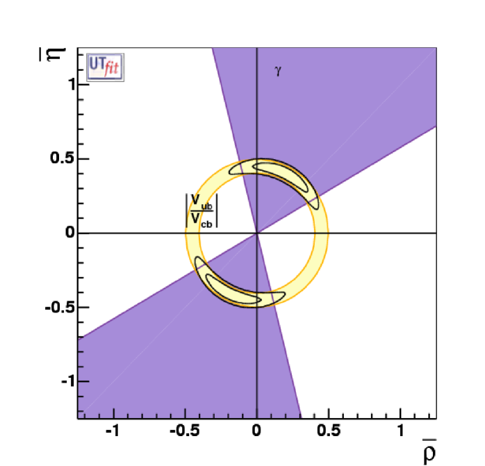
Figure 1: The selected region on $\bar{\rho}$-$\bar{\eta}$ plane obtained from the determination of $|V_{ub}/V_{cb}|$ and $\gamma$ (using $DK$ final states). Selected regions corresponding to $68\%$ and $95\%$ probability are shown, together with $95\%$ probability regions for $\gamma$ and $|V_{ub}/V_{cb}|$.

Let us first of all discuss the shape of the UT in the presence of arbitrary NP contributions. All the available experimental data exclude the possibility of sizable contributions to tree-level SM processes, so that extensions of the SM in which NP enters low-energy processes at the tree level are strongly disfavoured. We can therefore safely assume in this work that NP enters observables in the flavour sector only at the loop level. It is then possible to determine two regions in the $\bar{\rho}-\bar{\eta}$ plane independently of NP contributions, using only tree-level $B$ decays. The CKM elements $V_{ub}$ and $V_{cb}$ are determined using semileptonic inclusive and exclusive $B$ decays. The angle $\gamma$ is obtained by measuring the phase of $V_{ub}$ appearing in the interference between $b\to c$ and $b\to u$ transitions to $DK$ final states. As shown in Fig. 1, it is now lunchtime ($\sim$13:35) on Andrzej’s unitarity clock [21].

The results of this analysis, reported in Tab. 2, can be used as a reference for model-building and phenomenology in any extension of the SM with loop-mediated contributions to FCNC processes. The present precision is expected to improve considerably in the near future, as discussed in Sec. 6.

UT fit - using only $|V_{ub}/V_{cb}|$ and $\gamma$
	SM Solution	2nd Solution
$\bar{\rho}$	0.18 $\pm$ 0.12	-0.18 $\pm$ 0.12
$\bar{\eta}$	0.41 $\pm$ 0.05	-0.41 $\pm$ 0.05
$\sin 2\beta$	0.782 $\pm$ 0.065	-0.641 $\pm$ 0.087
$\gamma\,[^{\circ}]$	65 $\pm$ 18	-115 $\pm$ 18
$\alpha\,[^{\circ}]$	87$\pm$ 15	-46 $\pm$ 15
$2\beta+\gamma\,[^{\circ}]$	122 $\pm$ 13	-152 $\pm$ 13

Table 2: Results for several UT parameters, obtained using the constraints from $|V_{ub}/V_{cb}|$ and $\gamma$ (using $DK$ final states).

Beyond the Standard Model, one can include the information from other constraints, taking into account the effect of NP in a general way. In particular, one has to consider two effects:

• The contribution of new operators in the $|\Delta F|=2$ Hamiltonian, which affects mixing processes and, as a consequence, the determination of $\Delta m_{d,s}$, $\varepsilon_{K}$ and of the angles $\beta$ and $\alpha$.

• The effect of NP in the $|\Delta F|=1$ Hamiltonian, for all those processes occurring through penguin transitions. In our case, this concerns the determination of $\alpha$ from charmless $B$ decays and the CP asymmetry in semileptonic $B$ decays $A_{\mathrm{SL}}$.

3 Model-independent constraints on New Physics in $\mathbf{|\Delta F|}$=2 transitions

Our goal in this Section is to use the available experimental information on loop-mediated processes to constrain the NP contributions to $|\Delta F|$=2 transitions. In general, NP models introduce a large number of new parameters: flavour changing couplings, short distance coefficients and matrix elements of new local operators. The specific list and the actual values of these parameters can only be determined within a given model. Nevertheless, each of the mixing processes listed in Tab. 3 is described by a single amplitude and can be parameterized, without loss of generality, in terms of two parameters, which quantify the difference of the complex amplitude with respect to the SM one [22]. Thus, for instance, in the case of $B^{0}_{q}-\bar{B}^{0}_{q}$ mixing we define

$$C_{B_{q}}\,e^{2i\phi_{B_{q}}}=\frac{\langle B^{0}_{q}|H_{\mathrm{eff}}^{\mathrm{full}}|\bar{B}^{0}_{q}\rangle}{\langle B^{0}_{q}|H_{\mathrm{eff}}^{\mathrm{SM}}|\bar{B}^{0}_{q}\rangle}\,,\qquad(q=d,s)$$ (1)

where $H_{\mathrm{eff}}^{\mathrm{SM}}$ includes only the SM box diagrams, while $H_{\mathrm{eff}}^{\mathrm{full}}$ includes also the NP contributions. In the absence of NP effects, $C_{B_{q}}=1$ and $\phi_{B_{q}}=0$ by definition. The experimental quantities determined from the $B^{0}_{q}-\bar{B}^{0}_{q}$ mixings and listed in Tab. 3 are related to their SM counterparts and the NP parameters by the following relations:

$$\Delta m_{d}^{\mathrm{exp}}=C_{B_{d}}\Delta m_{d}^{\mathrm{SM}}\,,\;\sin 2\beta^{\mathrm{exp}}=\sin(2\beta^{\mathrm{SM}}+2\phi_{B_{d}})\,,\;\alpha^{\mathrm{exp}}=\alpha^{\mathrm{SM}}-\phi_{B_{d}}\,,$$ (2)

in a self-explanatory notation.

Tree-Level	B${}^{0}_{d}$ mixing	K0 mixing	B${}^{0}_{s}$ mixing
$|V_{ub}/V_{cb}|$	$\Delta{m_{d}}$	$\epsilon_{K}$	$\Delta m_{s}$
$\gamma$ ($DK$)	$A_{CP}(B\to J/\psi K)$		$A_{CP}(B^{0}_{s}\to J/\psi\phi)$
	$A_{CP}(B\to\pi\pi,\rho\pi,\rho\rho)$
	$A_{\mathrm{SL}}$

Table 3: Different processes and corresponding measurements contributing to the determination of $\bar{\rho}$, $\bar{\eta}$, $C_{B_{d}}$, $\phi_{B_{d}}$, $C_{B_{s}}$,$\phi_{B_{s}}$ and $C_{\varepsilon_{K}}$. $\Delta m_{K}$ is not considered due to the fact that the long distance effects are not well under control.

As far as the $K^{0}-\bar{K}^{0}$ mixing is concerned, we find it convenient to introduce a single parameter which relates the imaginary part of the amplitude to the SM one:

$$C_{\epsilon_{K}}=\frac{\mathrm{Im}[\langle K^{0}|H_{\mathrm{eff}}^{\mathrm{full}}|\bar{K}^{0}\rangle]}{\mathrm{Im}[\langle K^{0}|H_{\mathrm{eff}}^{\mathrm{SM}}|\bar{K}^{0}\rangle]}\,.$$ (3)

This definition implies in fact a simple relation for the measured value of $\varepsilon_{K}$,

$$\varepsilon_{K}^{\mathrm{exp}}=C_{\epsilon_{K}}\,\varepsilon_{K}^{\mathrm{SM}} \qquad(K^{0}-\bar{K}^{0}~{}\mathrm{mixing})\,.$$ (4)

$\Delta m_{K}$ is not considered because the long distance effects are not well under control. Therefore, all NP effects which enter the present analysis are parameterized in terms of three real quantities, $C_{B_{d}}$, $\phi_{B_{d}}$, and $C_{\epsilon_{K}}$. NP in the $B_{s}$ sector is not considered in this case, due to the lack of experimental information, since both $\Delta m_{s}$ and $A_{\mathrm{CP}}(B_{s}\to J/\psi\phi)$ are not measured yet.

3.1 New Physics effects in the extraction of $\mathbf{\alpha}$ from $\mathbf{|\Delta F|}$=1 processes

In principle, the extraction of $\alpha$ from $B\to\pi\pi,~{}\rho\pi,~{}\rho\rho$ decays is affected by NP effects in $|\Delta F|$=1 transitions. Actually, in the presence of NP in the strong $b\to d$ penguins, the decay amplitudes for $B$ mesons decaying into $\pi\pi$, $\rho\pi$ and $\rho\rho$ are a simple generalization of the SM ones (given for example in Eqs. (17) and (18) of Ref. [1]). We assume that NP modifies significantly only the “penguin” amplitude $P$ without changing its isospin quantum numbers (i.e. barring large isospin-breaking NP effects). Then, instead of a complex penguin amplitude with vanishing weak phase, we have two independent arbitrary complex penguin amplitudes for $B$ and $\bar{B}$ decays. For example, the amplitudes of $B\to\pi\pi(\rho\rho)$ can be written as

$$A^{+-} = -Te^{-i\alpha}+Pe^{i\phi_{P}}e^{i\delta_{P}}$$

$$\bar{A}^{+-} = -Te^{i\alpha}+\bar{P}e^{-i\phi_{P}}e^{i\delta_{P}}$$

$$A^{+0} = -\frac{1}{\sqrt{2}}\left[e^{-i\alpha}\left(T+T_{c}e^{i\delta_{T_{c}}}\right)\right]$$

$$\bar{A}^{-0} = -\frac{1}{\sqrt{2}}\left[e^{i\alpha}\left(T+T_{c}e^{i\delta_{T_{c}}}\right)\right]$$

$$A^{00} = -\frac{1}{\sqrt{2}}\left[T_{c}e^{-i\alpha}e^{i\delta_{T_{c}}}+Pe^{i\phi_{P}}e^{i\delta_{P}}\right]\,,$$

$$\bar{A}^{00} = -\frac{1}{\sqrt{2}}\left[T_{c}e^{i\alpha}e^{i\delta_{T_{c}}}+Pe^{-i\phi_{P}}e^{i\delta_{P}}\right]\,,$$ (5)

where $T$, $T_{c}$, $P$ and $\bar{P}$ are real parameters, $\delta_{P}$ and $\delta_{T_{c}}$ are strong phases, $\alpha$ is the angle of the UT, and $\phi_{P}$ is an additional weak phase.

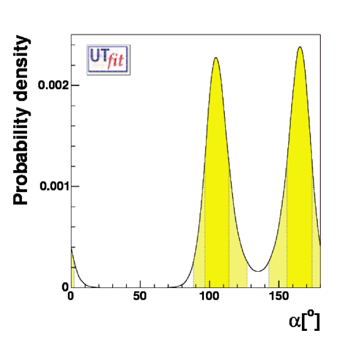
Figure 2: P.d.f. of $\alpha$ from the combination of isospin analyses of $\pi\pi$, $\rho\pi$ and $\rho\rho$ decay modes, including NP effects in the $|\Delta F|=1$ Hamiltonian.

The procedure to extract $\alpha$ is exactly the same as in the SM [1], since we assume that NP does not affect the $\Delta I=3/2$ amplitudes. However, in the NP fit we lose the knowledge of the weak phase of the penguins. In spite of this additional free parameter, the experimental information available nowadays is sufficient to constrain $\alpha$ even in the presence of NP, as shown in Fig. 2. We take $T$, $T_{c}$, $P$ and $\bar{P}$ to be flatly distributed in a range larger than the one determined from the fit, and all the phases to be flatly distributed in the $[0,2\pi)$ range. Here and in the following figures, dark (light) areas correspond to the $68\%$ ($95\%$) probability region. One should notice that these analyses bound $\alpha$ through the quantity $\pi-\beta-\gamma$, where $\gamma$ comes from the decay amplitudes and $\beta$ from $B_{d}-\bar{B}_{d}$ mixing. Therefore, in the presence of NP effects in the $|\Delta F|=2$ Hamiltonian, this bound should be regarded as a constraint on $\alpha^{\mathrm{SM}}-\phi_{B_{d}}$ (see Eq. 2).

The reader might notice a contradiction between the discussion above and the results of ref. [23, 15], in which it is stated that the NP parameters introduced above can be eliminated by a redefinition of the $T$, $T_{c}$ and $P$ parameters. Explicitly, one has

$$A^{+-} = -T_{X}e^{-i\alpha}+P_{X}$$

$$A^{+0} = -\frac{1}{\sqrt{2}}\left[e^{-i\alpha}\left(T_{X}+T_{cX}\right)\right]$$

$$A^{00} = -\frac{1}{\sqrt{2}}\left[T_{cX}e^{-i\alpha}+P_{X}\right]\,,$$ (6)

with

$$T_{X} = T+\frac{Pe^{i\phi_{P}}-\bar{P}e^{-i\phi_{P}}}{2i\sin\alpha}e^{i\delta_{P}}$$ (7)

$$T_{cX} = T_{c}e^{i\delta_{T_{c}}}-\frac{Pe^{i\phi_{P}}-\bar{P}e^{-i\phi_{P}}}{2i\sin\alpha}e^{i\delta_{P}}$$

$$P_{X} = \frac{Pe^{i(\alpha+\phi_{P})}-\bar{P}e^{-i(\alpha+\phi_{P})}}{2i\sin\alpha}e^{i\delta_{P}}\,.$$

However, the transformations (7) are singular for $\alpha\to 0$. This implies that there is no limited a-priori range for the $X$ parameters. For this reason, the parameterization in eq. (5) is of no use for our purpose.

3.2 $\mathbf{A_{\mathrm{SL}}}$: general considerations and the inclusion of $\mathbf{|\Delta F|}$=1 New Physics effects

One can also add the constraint coming from the CP asymmetry in semileptonic $B$ decays $A_{\mathrm{SL}}$, defined as

$$A_{\mathrm{SL}}\equiv\frac{\Gamma(\bar{B}^{0}\to\ell^{+}X)-\Gamma(B^{0}\to\ell^{-}X)}{\Gamma(\bar{B}^{0}\to\ell^{+}X)+\Gamma(B^{0}\to\ell^{-}X)}\,.$$ (8)

It has been noted in Ref. [13] that, even though the present experimental bound is not precise enough to bound $\bar{\rho}$ and $\bar{\eta}$ in the Standard Model, $A_{\mathrm{SL}}$ is a crucial ingredient of the UT analysis once the formulae are generalized according to Eq. (2), since this is the only constraint that depends on both $C_{B_{d}}$ and $\phi_{B_{d}}$:

$$A_{\mathrm{SL}}=-\mathrm{Re}\left(\frac{\Gamma_{12}}{M_{12}}\right)^{\mathrm{SM}}\frac{\sin 2\phi_{B_{d}}}{C_{B_{d}}}+\mathrm{Im}\left(\frac{\Gamma_{12}}{M_{12}}\right)^{\mathrm{SM}}\frac{\cos 2\phi_{B_{d}}}{C_{B_{d}}}\,,$$ (9)

where $\Gamma_{12}$ and $M_{12}$ are the absorptive and dispersive parts of the $B^{0}_{d}-\bar{B}^{0}_{d}$ mixing amplitude. At the leading order, $A_{\mathrm{SL}}$ is independent of penguin operators, and therefore it is also independent of NP in $|\Delta F|=1$ processes. However, at the NLO, the penguin contribution should be taken into account. In the SM, the effect of penguin operators is GIM suppressed since their CKM factor is aligned with $M_{12}$: both are proportional to $(V_{tb}^{*}V_{td})^{2}$. This is not true anymore in the presence of NP, so that the effects of penguins are amplified beyond the SM and the approximation made in Ref. [13] of neglecting this contribution is questionable. For our analysis of $A_{\mathrm{SL}}$, we therefore start from the full NLO calculation of Ref. [24], allowing for an additional NP contribution to the penguin term in the $|\Delta F|=1$ amplitude. This introduces two additional parameters ($C_{\mathrm{Pen}}$ and $\phi_{\mathrm{Pen}}$), encoding NP contributions to the penguin part in analogy to what $C_{B_{d}}$ and $\phi_{B_{d}}$ do for the box contribution. Since the penguin amplitude is $\mathcal{O}(\alpha_{s})$ with respect to the leading contribution, these parameters introduce a smearing in the theoretical determination of $A_{\mathrm{SL}}$. The generalized expression of $A_{\mathrm{SL}}$ is given by

$$A_{\mathrm{SL}} = -\frac{2\kappa}{C_{B_{d}}}\left\{\sin\left(2\phi_{B_{d}}\right)\left(n_{1}+\frac{n_{6}B_{2}+n_{11}}{B_{1}}\right)-\frac{\sin\left(\beta+2\phi_{B_{d}}\right)}{R_{t}}\left(n_{2}+\frac{n_{7}B_{2}+n_{12}}{B_{1}}\right)\right.$$ (10)

$$+\frac{\sin\left(2(\beta+\phi_{B_{d}})\right)}{R_{t}^{2}}\left(n_{3}+\frac{n_{8}B_{2}+n_{13}}{B_{1}}\right)+\sin\left(\phi_{\mathrm{Pen}}+2\phi_{B_{d}}\right)C_{\mathrm{Pen}}\left(n_{4}+n_{9}\frac{B_{2}}{B_{1}}\right)$$

$$\left.-\sin\left(\beta+\phi_{\mathrm{Pen}}+2\phi_{B_{d}}\right)\frac{C_{\mathrm{Pen}}}{R_{t}}\left(n_{5}+n_{10}\frac{B_{2}}{B_{1}}\right)\right\}$$

where $B_{1}$ corresponds to the usual $B_{d}$ parameter for $B^{0}-\bar{B}^{0}$ mixing, $B_{2}=0.84\pm 0.07$ (flat) [25], $R_{t}=\sqrt{(1-\bar{\rho})^{2}+\bar{\eta}^{2}}$ is the length of one of the UT sides, $\kappa$ is defined in Ref. [24] and the magic numbers $n_{i}$ are given in Tab. 4. The Standard Model expression can be recovered in the limit $C_{X}\to 1$ and $\phi_{X}\to 0$ (where $X=B_{d}$, Pen). Eq. (10) contains NLO QCD and $1/m_{b}$ corrections; the latter have been estimated using matrix elements computed in the vacuum insertion approximation, since lattice results are not available.

$n_{1}$	$0.1797\pm 0.0017$	$n_{2}$	$0.1391\pm 0.0193$	$n_{3}$	$-0.0012\pm 0.0014$
$n_{4}$	$-0.0074\pm 0.0020$	$n_{5}$	$0.0020\pm 0.0007$	$n_{6}$	$1.0116\pm 0.0826$
$n_{7}$	$0.0455\pm 0.0144$	$n_{8}$	$-0.0004\pm 0.0046$	$n_{9}$	$-0.0714\pm 0.0170$
$n_{10}$	$-0.0041\pm 0.0016$	$n_{11}$	$-0.3331\pm 0.2178$	$n_{12}$	$0.0028\pm 0.0101$
$n_{13}$	$-0.0036\pm 0.0033$

Table 4: Magic numbers for the calculation of $A_{\mathrm{SL}}$. The quoted errors correspond to Gaussian distributions.

To display the main phenomenological consequences of $A_{SL}$, let us consider a simplified formula obtained by setting all magic numbers to their central values, and dropping all those smaller than $10^{-2}$. In this way we get

$$A_{\mathrm{SL}} \sim \frac{2\kappa}{C_{B_{d}}}\left\{\sin\left(2\phi_{B_{d}}\right)\left(0.18+\frac{1.01B_{2}-0.33}{B_{1}}\right)-\frac{\sin\left(\beta+2\phi_{B_{d}}\right)}{R_{t}}\left(0.14+0.05\frac{B_{2}}{B_{1}}\right)\right.$$ (11)

$$\left.+\sin\left(\phi_{\mathrm{Pen}}+2\phi_{B_{d}}\right)C_{\mathrm{Pen}}(-0.07)\frac{B_{2}}{B_{1}}\right\}\,.$$

The SM penguin contribution vanishes at this level of accuracy. It is evident from the simplified expression in Eq. (11) that the phase $\phi_{B_{d}}$ can induce an order-of-magnitude enhancement of $A_{\mathrm{SL}}$ relative to the SM, while the penguin phase $\phi_{\mathrm{Pen}}$ can induce corrections comparable to the SM contribution. To be conservative, for our analysis we varied $C_{\mathrm{Pen}}$ in the range $[0,2]$ with $\phi_{\mathrm{Pen}}\in[0,2\pi]$. This produces only a minor smearing of the dominant effects due to NP in $|\Delta B|=2$ transitions.

3.3 Results of the analysis and constraints on $\mathbf{|\Delta F|=2}$ NP contributions

To obtain the constraints on NP we extract $C_{B_{d}}$, $C_{\epsilon_{K}}$, $\bar{\rho}$ and $\bar{\eta}$ with a flat distribution in a range much larger than the experimentally allowed region. The phase $\phi_{B_{d}}$ is taken to be flatly distributed in the range $[0,\pi]$. The generated events are weighted using the experimental information on $|V_{ub}/V_{cb}|$, $B\to DK$ decays ($\gamma$), $\epsilon_{K}$, $B\to\rho\rho$, $\rho\pi$, and $\pi\pi$ decays ($\alpha$), $B\to J/\Psi K^{(*)}$ and $B\to D^{0}h^{0}$ decays [26, 27] ($\beta$), and $A_{\mathrm{SL}}$ [18], using the technique described in ref. [17]. The output p.d.f.’s for $C_{B_{d}}$, $C_{\epsilon_{K}}$, $C_{B_{d}}$ vs. $\phi_{B_{d}}$, and $\gamma$ vs. $\phi_{B_{d}}$ are shown in Fig. 3, and the corresponding regions in the $\bar{\rho}$–$\bar{\eta}$ plane are presented in Fig. 4.

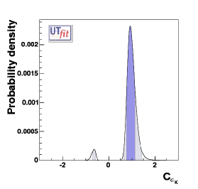
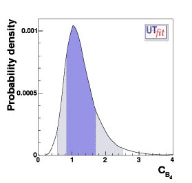
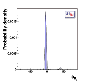
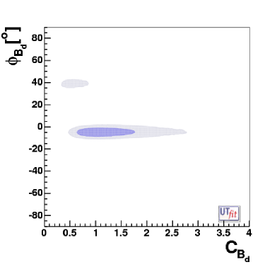
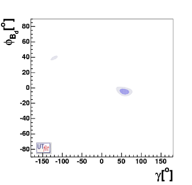
Figure 3: Output P.d.f.’s for $C_{\epsilon_{K}}$ (top-left),$C_{B_{d}}$ (top-center), $\phi_{B_{d}}$ (top-right), and 2D distributions of $\phi_{B_{d}}\,vs.\,C_{B_{d}}$ (bottom-left) and $\phi_{B_{d}}\,vs.\,\gamma$. Dark (light) areas correspond to the $68\%$ ($95\%$) probability region.

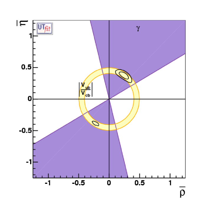
Figure 4: The selected region on $\bar{\rho}$-$\bar{\eta}$ plane obtained from the NP generalized analysis. Selected regions corresponding to $68\%$ and $95\%$ probability are shown, together with $95\%$ probability regions for $\gamma$ (from $DK$ final states) and $|V_{ub}/V_{cb}|$.

It is important to remark that the constraints coming from the experimental observables allow for an increase in the precision on $\bar{\rho}$ and $\bar{\eta}$ with respect to the pure tree-level determination. This is clear comparing Fig. 1 to Fig. 4.

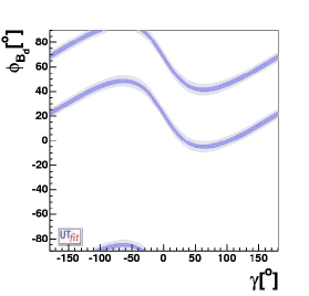
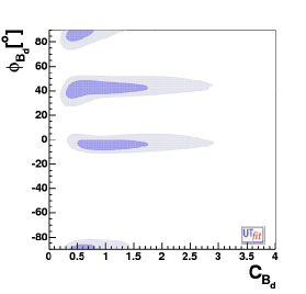
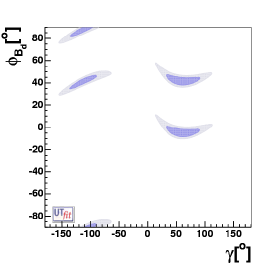
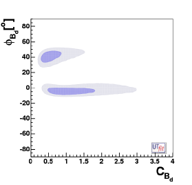
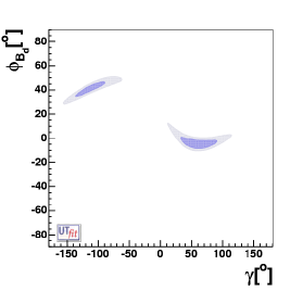
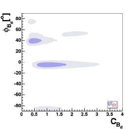
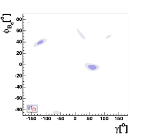
Figure 5: 2D distributions of $\phi_{B_{d}}$ vs. $C_{B_{d}}$ (left) and $\phi_{B_{d}}$vs. $\gamma$ (right) using the following constraints: i) $|V_{ub}/V_{cb}|$, $\Delta m_{d}$, $\varepsilon_{K}$ and $\sin 2\beta$ (first row); ii) the constraints in i) plus $\gamma$ (second row); iii) the constraints in ii) plus $\cos 2\beta$ from $B_{d}\to J/\psi K^{*}$ and $\beta$ from $B\to Dh^{0}$ (third row); iv) the constraints in ii) plus $\alpha$ (fourth row).

To illustrate the impact of each experimental constraint on the analysis, in Fig. 5 we show the selected regions in the $\phi_{B_{d}}$ vs. $C_{B_{d}}$ and $\phi_{B_{d}}$ vs. $\gamma$ planes using different combinations of constraints. The first row represents the pre-2004 situation, when only $|V_{ub}/V_{cb}|$, $\Delta m_{d}$, $\varepsilon_{K}$ and $\sin 2\beta$ were available, selecting a continuous band for $\phi_{B_{d}}$ as a function of $\gamma$ and a broad region for $C_{B_{d}}$. Adding the determination of $\gamma$ (second row), only four regions in the $\phi_{B_{d}}$ vs. $\gamma$ plane survive, two of which overlap in the $\phi_{B_{d}}$ vs. $C_{B_{d}}$ plane. Two of these solutions have values of $\cos 2(\beta+\phi_{B_{d}})$ and $\alpha-\phi_{B_{d}}$ different from the SM predictions, and are therefore disfavoured by $(\cos 2\beta)^{\mathrm{exp}}$ and by the measurement of $(2\beta)^{\mathrm{exp}}$ from $B\to Dh^{0}$ decays, and by $\alpha^{\mathrm{exp}}$ (third and fourth row respectively). On the other hand, the third solution has a very large value for $A_{\mathrm{SL}}$ and is therefore disfavoured by $A_{\mathrm{SL}}^{\mathrm{exp}}$, leading to the final results already presented in Fig. 3.

Generalized UTfit analysis in the presence of NP
	Standard Solution $(\gamma>0)$	Non-Standard Solution $(\gamma<0)$
UT parameters
$\bar{\rho}$	0.246 $\pm$ 0.053 ([0.115, 0.370] @95$\%$)	[-0.230, -0.212] @95$\%$
$\bar{\eta}$	0.379 $\pm$ 0.039 ([0.277, 0.463] @95$\%$)	[-0.398, -0.381] @95$\%$
$\sin 2\beta$	0.799 $\pm$ 0.037 ([0.694, 0.880] @95$\%$)	[-0.588, -0.574] @95$\%$
$\gamma$ $[^{\circ}]$	$57.1\pm 7.8$ ([37.9, 75.4] @95$\%$)	[-121.5, -118.4] @95$\%$
$\alpha$ $[^{\circ}]$	$96.0\pm 8.4$ ([78.3, 116.5] @95$\%$)	[-44.5,  -40.0] @95$\%$
$2\beta+\gamma$ $[^{\circ}]$	$110.9\pm 9.2$ ([88.8,  128.6] @95$\%$)	[-158.5, -153.0] @95$\%$
Im $\lambda_{t}$ [$\times 10^{-5}$]	$14.9\pm 1.5$ ([11.7, 17.6] @95$\%$)
$\Delta m_{s}$ [ps-1]	$18.0\pm 5.3$([8.9, 29.6] @95$\%$)
NP related parameters
$C_{B_{d}}$	$1.27\pm 0.44$ ([0.56, 2.51] @95$\%$)
$\phi_{B_{d}}[^{\circ}]$	$-4.7\pm 2.3$ ([-9.9, 1.0] @95$\%$)	[39.0, 39.8] @95$\%$
$C_{\epsilon_{K}}$	$0.95\pm 0.18$ ([0.64, 1.44] @95$\%$)	[-0.71, -0.59] @95$\%$

Table 5: Results of the NP generalized analysis on UT parameters. The values for $C_{B_{d}}$, $\phi_{B_{d}}$ and $C_{\epsilon_{K}}$ are reported. The second solution is excluded at 68$\%$ probability level so we quote the $95\%$ ranges only.

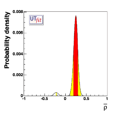
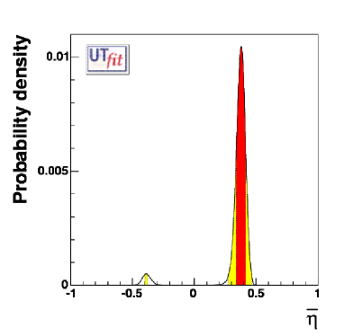
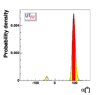
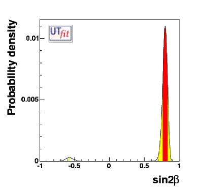
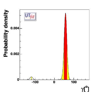
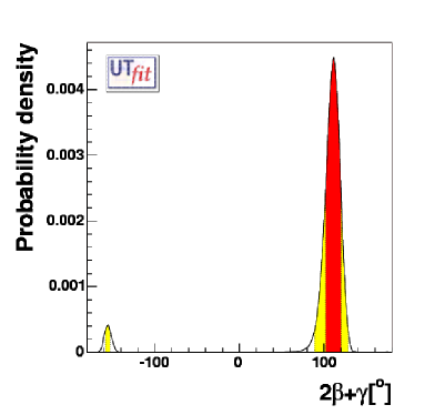
Figure 6: From top to bottom and from left to right, the p.d.f.’s for $\bar{\rho}$, $\bar{\eta}$, $\alpha$, $\sin 2\beta$, $\gamma$ and $2\beta+\gamma$. The red (darker) and the yellow (lighter) zones correspond respectively to 68% and 95% of the area. These results are obtained in the presence of NP in all the processes entering the UT analysis.

In Tab. 5 we give the numerical results for the NP parameters and some of the relevant UT quantities, for which we show the output distributions in Fig. 6. A comment is needed for the case of $\Delta m_{s}$: the output distribution reported in Fig. 7 represents the SM contribution only (i.e. it corresponds to $C_{B_{s}}=1$). Therefore this numerical result should not be taken as a prediction for $\Delta m_{s}$ in a general NP scenario in which $C_{B_{s}}\neq 1$. The conclusion that we can draw from the output distribution of $\Delta m_{s}$ is most easily read from the compatibility plot shown in Fig. 7: a value of $\Delta m_{s}>30\,(36)$ ps^-1 would imply the presence of NP in $B_{s}-\bar{B}_{s}$ mixing at the $2\,(3)\,\sigma$ level. On the other hand, from the similar result in the contest of the Standard Model [1] one can still conclude that $\Delta m_{s}>29\,(34)$ ps^-1 would imply the presence of NP at the $2\,(3)\,\sigma$ level (but not necessarily in the $B_{s}$ sector).

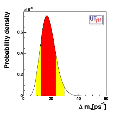
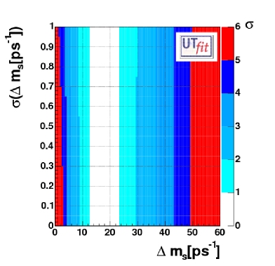
Figure 7: P.d.f. (left) and compatibility plot (right) for the SM contribution to $\Delta m_{s}$ in the presence of NP in all the quantities entering the UT analysis, setting $C_{B_{s}}=1$.

Before concluding this section, let us analyze more in detail the results in Fig. 3. Writing

$$C_{B_{d}}e^{2i\phi_{B_{d}}}=\frac{A_{\mathrm{SM}}e^{2i\beta}+A_{\mathrm{NP}}e^{2i(\beta+\phi_{\mathrm{NP}})}}{A_{\mathrm{SM}}e^{2i\beta}}\,,$$ (12)

and given the p.d.f. for $C_{B_{d}}$ and $\phi_{B_{d}}$, we can derive the p.d.f. in the $(A_{\mathrm{NP}}/A_{\mathrm{SM}})$ vs. $\phi_{\mathrm{NP}}$ plane. The result is reported in Fig. 8. We see that the NP contribution can be substantial if its phase is close to the SM phase, while for arbitrary phases its magnitude has to be much smaller than the SM one. Notice that, with the latest data, the SM ($\phi_{B_{d}}=0$) is disfavoured at $68\%$ probability due to a slight disagreement between $\sin 2\beta$ and $|V_{ub}/V_{cb}|$. This requires $A_{\mathrm{NP}}\neq 0$ and $\phi_{\mathrm{NP}}\neq 0$. For the same reason, $\phi_{\mathrm{NP}}>90^{\circ}$ at $68\%$ probability and the plot is not symmetric around $\phi_{\mathrm{NP}}=90^{\circ}$.

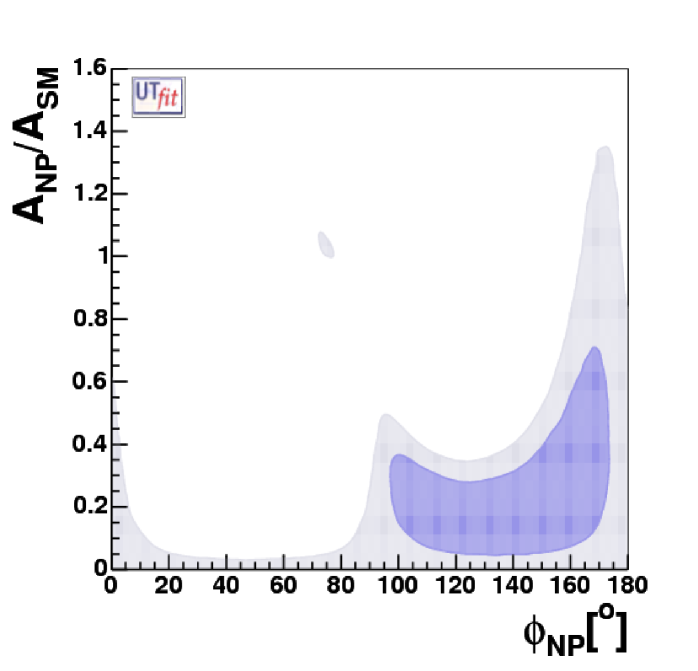
Figure 8: P.d.f. in the $(A_{\mathrm{NP}}/A_{\mathrm{SM}})$ vs. $\phi_{\mathrm{NP}}$ plane for NP in the $|\Delta B|=2$ sector (see Eq. (12)).

A similar parameterization has been used in ref. [28]. Comparing our Fig. 8 with Fig. 5 of ref. [28], one notices small differences. However, since they are using the statistical method of ref. [15], they are plotting areas corresponding to “at least” confidence levels, so that their areas are expected to be larger than ours.

Assuming that the small but non-vanishing value for $\phi_{B_{d}}$ we obtained is just due to a statistical fluctuation, the result of our analysis points either towards models in which new sources of flavour and CP violation are only present in $b\to s$ transitions, a well-motivated possibility in flavour models and in grand-unified models, or towards models with no new source of flavour and CP violation beyond the ones present in the SM (Minimal Flavour Violation). This second possibility will be studied in detail in Section 5.

4 Constraints on NP from $\mathbf{|\Delta S|=2}$ or $\mathbf{|\Delta B|=2}$ transitions only

A complementary information to the one presented in the previous section is obtained by allowing NP contributions to be present only in $|\Delta S|=2$ or $|\Delta B|=2$ transitions. This can be useful to test models beyond the SM in which NP contributions are expected to affect dominantly only one of these two sectors, and is also the starting point to update previous analyses of NP in $|\Delta S|=2$ or $|\Delta B|=2$ processes in supersymmetry [29, 30] or in any other given model.

Allowing NP to affect only $C_{\varepsilon_{K}}$, we obtain the results for the UT parameters, for $C_{\varepsilon_{K}}$ and for $\bar{\rho}$ and $\bar{\eta}$ reported in Fig. 9 and in Tab. 6. The determination of the UT is essentially equivalent to the SM one, since only $\varepsilon_{K}$ is missing in this case.

For the case in which NP only enters $B_{d}-\bar{B}_{d}$ mixing, the results are given in Fig. 10 and in Tab. 6. The main difference with the results in the previous section is that one can use $\varepsilon_{K}$ to eliminate the solutions with negative $\gamma$.

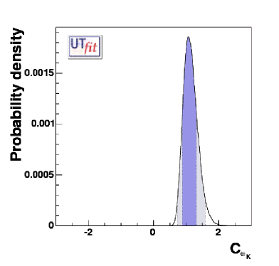
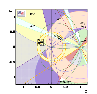
Figure 9: The p.d.f. for $C_{\varepsilon_{K}}$ (left) and the $\bar{\rho}-\bar{\eta}$ plane (right). In the left plot, the darker and the lighter zones correspond respectively to 68% and 95% of the area. These results are obtained in the presence of NP in $K^{0}-\bar{K}^{0}$ mixing only.

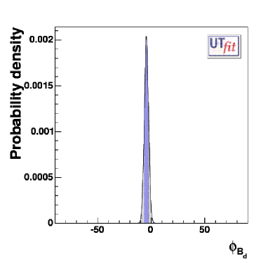
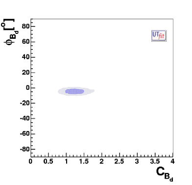
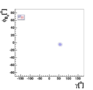
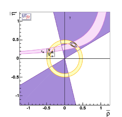
Figure 10: From top to bottom and from left to right, the p.d.f.’s for $C_{B_{d}}$, $\phi_{B_{d}}$, $\phi_{B_{d}}$ vs. $C_{B_{d}}$, $\phi_{B_{d}}$ vs. $\gamma$ and the $\bar{\rho}-\bar{\eta}$ plane. The darker and the lighter zones correspond respectively to 68% and 95% of the area. These results are obtained in the presence of NP in $B^{0}_{d}-\bar{B}^{0}_{d}$ mixing only.

Generalized UTfit analysis in the presence of NP
	$|\Delta S|=2$ only	$|\Delta B_{d}|=2$ only
UT parameters
$\bar{\rho}$	0.267 $\pm$ 0.056 [0.145,0.368]	0.246 $\pm$ 0.038 [0.166,0.317]
$\bar{\eta}$	0.319 $\pm$ 0.034 [0.257,0.387]	0.372 $\pm$ 0.028 [0.318,0.424]
$\sin 2\beta$	0.730 $\pm$ 0.028 [0.674,0.781]	0.794 $\pm$ 0.033 [0.727,0.854]
$\gamma$ $[^{\circ}]$	$50\pm 9$ [35,69]	$56\pm 5$ [46,67]
$\alpha$ $[^{\circ}]$	$107\pm 9$ [87,123]	$97\pm 6$ [86,108]
$2\beta+\gamma$ $[^{\circ}]$	$100\pm 10$ [80,118]	$109\pm 6$[96,120]
Im $\lambda_{t}$ [$\times 10^{-5}$]	$12.6\pm 1.4$ [10.1,15.4]	$14.9\pm 1.0$ [13.0,16.8]
$\Delta m_{s}$ [ps-1]	$22.6\pm 4.2$ [15.2,30.8]	$17.4\pm 2.0$ [14.8,22.4]
NP related parameters
$C_{B_{d}}$	1	1.25 $\pm$ 0.21 [0.84,1.69]
$\phi_{B_{d}}$ $[^{\circ}]$	0	$-4.6\pm 2.0$ [-8.5,-0.7]
$C_{\epsilon_{K}}$	$1.10\pm 0.21$ [0.73,1.59]	1

Table 6: Results of the NP generalized analysis on UT parameters, when only NP contributions to the $|\Delta S|=2$ (left) and $|\Delta B_{d}|=2$ (right) processes are considered. The values for $C_{B_{d}}$, $\phi_{B_{d}}$ and $C_{\epsilon_{K}}$ are reported. The quoted errors represent 68$\%$ [95%] probability ranges.

5 Minimal Flavour Violation models

We now specialize to the case of MFV. Making the basic assumption that the only source of flavour and CP violation is in the Yukawa couplings [6], it can be shown that:

1. The phase of $|\Delta B|=2$ amplitudes is unaffected by NP, and so is the ratio $\Delta m_{s}/\Delta m_{d}$. This allows the determination of the Universal Unitarity Triangle independent on NP effects, based on $|V_{ub}/V_{cb}|$, $\gamma$, $A_{CP}(B\to J/\Psi K^{(*)})$, $\beta$ from $B\to D^{0}h^{0}$, $\alpha$, and $\Delta m_{s}/\Delta m_{d}$ [5].

2. For one-Higgs-doublet models, and for two-Higgs-doublet models at low $\tan\beta$, all NP effects in the UT analysis amount to a redefinition of the top box contribution to $|\Delta F|=2$ processes $S_{0}(x_{t})\to S_{0}(x_{t})+\delta S_{0}$.

3. For two-Higgs-doublet models with large $\tan\beta$, NP enters in a similar way with respect to the low $\tan\beta$ case, but this time one cannot relate the parameter redefining $S_{0}(x_{t})$ in the $B$ sector to the similar term in the $K$ sector. Therefore, two different redefinitions must be made for the $B$ and $K$ sectors: $S_{0}(x_{t})\to S_{0}(x_{t})+\delta S_{0}^{B,K}$.

We perform three different analyses, corresponding to the points 1.-3. above. First, we present the determination of the UUT, which is independent of NP contributions (Sec. 5.1) in the context of MFV models. Then we add to the analysis the NP parameter $\delta S_{0}$ and constrain it, together with $\bar{\rho}$ and $\bar{\eta}$, using also the neutral meson mixing amplitudes. Finally, we consider the case $\delta S_{0}^{B}\neq\delta S_{0}^{K}$ and determine the constraints on $\bar{\rho}$, $\bar{\eta}$ and these NP parameters. We take $\delta S_{0}$, $\delta S_{0}^{B}$ and $\delta S_{0}^{K}$ to be flatly distributed in a range much larger than the experimentally allowed region.

5.1 Universal Unitarity Triangle

In Fig. 11 we show the allowed region in the $\bar{\rho}-\bar{\eta}$ plane for the UUT, and in Fig. 12 we plot the p.d.f.’s for several UT quantities. The corresponding values and ranges are reported in Tab. 7. The most important differences with respect to the general case are that i) the lower bound on $\Delta m_{s}$ forbids the solution in the third quadrant, and ii) the constraint from $\sin 2\beta$ is now effective, so that we are left with a region very similar to the SM one (for the reader’s convenience, we also report results of the SM UT analysis in Tab. 7). The values in Tab. 7 are the starting point for any study of rare decays and CP violation in MFV models. See Ref. [10] for a recent analysis based on the results of this work.

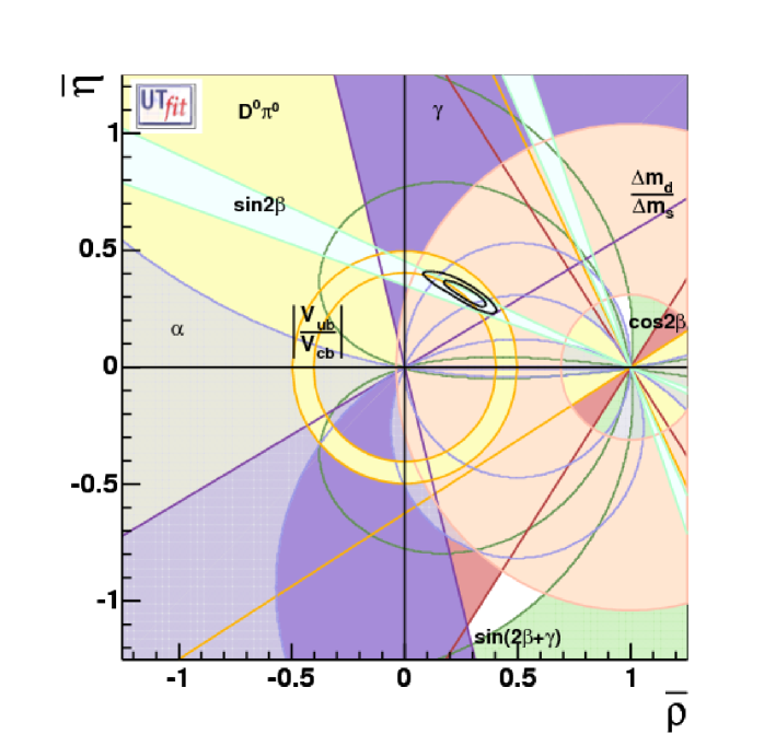
Figure 11: The selected region on $\bar{\rho}$-$\bar{\eta}$ plane obtained from the determination of the UUT.

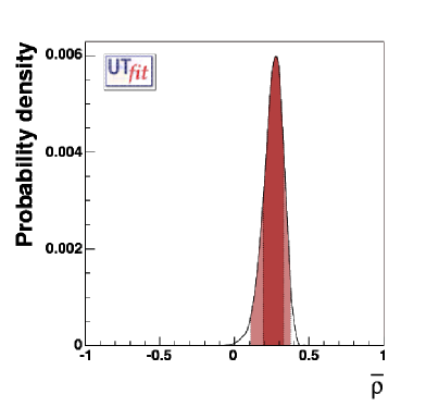
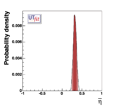
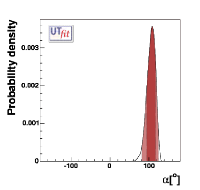
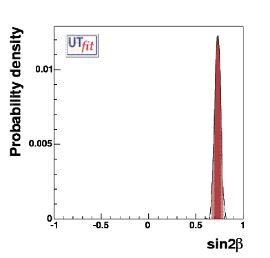
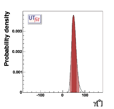
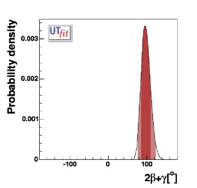
Figure 12: From top to bottom and from left to right, the p.d.f.’s for $\bar{\rho}$, $\bar{\eta}$, $\alpha$, $\sin 2\beta$, $\gamma$ and $2\beta+\gamma$. The red (darker) and the yellow (lighter) zones correspond respectively to 68% and 95% of the area. These results are obtained from the UUT analysis.

Universal Unitarity Triangle analysis
	UUT ($68\%$)	UUT ($95\%$)	SM ($68\%$)	SM ($95\%$)
UT parameters
$\bar{\rho}$	0.259 $\pm$ 0.068	$[0.107,\,0.376]$	0.216$\pm$ 0.036	$[0.143,\,0.288]$
$\bar{\eta}$	0.320 $\pm$ 0.042	$[0.241,\,0.399]$	0.342$\pm$0.022	$[0.300,\,0.385]$
$\sin 2\beta$	0.728 $\pm$ 0.031	$[0.668,\,0.778]$	0.735$\pm$ 0.024	$[0.688,\,0.781]$
$\alpha[^{\circ}]$	105 $\pm$ 11	$[81,\,124]$	98.5$\pm$ 5.7	$[87.1,\,109.8]$
$\gamma[^{\circ}]$	51 $\pm$ 10	$[33,\,75]$	57.6$\pm$ 5.5	$[46.8,\,68.7]$
$(2\beta+\gamma)[^{\circ}]$	98 $\pm$ 12	$[77,\,123]$	105.3$\pm$ 8.1	$[89.6,\,121.4]$
Im $\lambda_{t}$ [$\times 10^{-5}$]	12.7 $\pm$ 1.7	$[9.7,\,15.9]$	13.5 $\pm$ 0.8	$[12.0,\,15.0]$
$\Delta m_{s}$ [ps-1]	20.6 $\pm$ 5.6	$[10.6,\,32.6]$	20.0 $\pm$ 1.8	$[15.5,\,24.2]$

Table 7: Results of the UUT analysis. For convenience, the SM results from Ref. [1] are also reported.

5.2 Constraints on NP contributions in MFV models

We now determine the allowed ranges of NP contributions to $|\Delta F|=2$ processes, both in the small and large $\tan\beta$ regime. Furthermore, using the conventions of Ref. [6], we quantify the scale of NP that can be probed with the UT analysis.

Let us start by considering MFV models with one Higgs doublet or low/moderate $\tan\beta$. In this case, all NP effects in $|\Delta F|=2$ transitions are due to the effective Hamiltonian

$$\frac{a}{\Lambda^{2}}\frac{1}{2}\left(\bar{Q}_{L}\lambda_{FC}\gamma_{\mu}Q_{L}\right)^{2}\,,$$ (13)

with $(\lambda_{FC})_{ij}=Y_{t}^{2}V^{*}_{ti}V_{tj}$ for $i\neq j$ and zero otherwise, $Y_{t}$ the top quark Yukawa coupling, $\Lambda$ the scale of NP and $a$ an unknown (but real) Wilson coefficient. The value of $a$ can range from order one for strongly interacting extensions of the SM to much smaller values for weakly interacting theories and/or symmetry suppressions analogous to the GIM mechanism in the SM. It is now trivial to project this onto the SM $|\Delta F|=2$ effective Hamiltonian: it amounts only to a modification of the top quark contribution to box diagrams. Normalizing the NP Wilson coefficient to the SM effective electroweak scale $\Lambda_{0}=Y_{t}\sin^{2}\theta_{W}M_{W}/\alpha\approx 2.4$ TeV, we obtain

$$S_{0}(x_{t})\to S_{0}(x_{t})+\delta S_{0}\,,\qquad\delta S_{0}=4a\left(\frac{\Lambda_{0}}{\Lambda}\right)^{2}.$$ (14)

We can therefore determine simultaneously the shape of the UT and $\delta S_{0}$ from the standard UT analysis. Then, choosing as reference values $a=\pm 1$, we can translate the constraints on $\delta S_{0}$ into a lower bound on $\Lambda$. We obtain (see Fig. 13):

$$\Lambda>\left\{\begin{array}[]{l}3.6\mathrm{~{}TeV~{}@95\%~{}Prob.~{}for~{}positive~{}}\delta S_{0}\\ 5.1\mathrm{~{}TeV~{}@95\%~{}Prob.~{}for~{}negative~{}}\delta S_{0}\\ \end{array}\right.$$ (15)

Also in this case, we can obtain predictions for UT parameters, together with a constraint on NP contributions (see Tab. 8).

Minimal Flavour Violation analysis
	low/moderate $\tan\beta$		large $\tan\beta$
	$68\%$	$95\%$	$68\%$	$95\%$
$\bar{\rho}$	0.216 $\pm$ 0.058	$[0.109,\,0.361]$	0.231$\pm$ 0.067	$[0.112,\,0.375]$
$\bar{\eta}$	0.351 $\pm$ 0.032	$[0.265,\,0.406]$	0.347$\pm$0.036	$[0.254,\,0.404]$
$\sin 2\beta$	0.733 $\pm$ 0.027	$[0.679,\,0.781]$	0.731$\pm$ 0.027	$[0.673,\,0.781]$
$\alpha[^{\circ}]$	98.6 $\pm$ 9.5	$[81.6,\,121.7]$	101$\pm$ 11	$[82,\,124]$
$\gamma[^{\circ}]$	57.6 $\pm$ 9.1	$[35.7,\,79.1]$	55$\pm$ 11	$[34,\,74]$
$(2\beta+\gamma)[^{\circ}]$	104 $\pm$ 10	$[80,\,122]$	102$\pm$ 12	$[77,\,121]$
Im $\lambda_{t}$ [$\times 10^{-5}$]	13.6 $\pm$ 1.4	$[10.1,\,16.0]$	13.4 $\pm$ 1.9	$[9.7,\,16.3]$
$\Delta m_{s}$ [ps-1]	19.5 $\pm$ 2.6	$[15.0,\,31.7]$	22.6 $\pm$ 5.4	$[15.5,\,35.1]$

Table 8: Results for UT parameters from the MFV generalized analysis.

In the case of large $\tan\beta$, the situation changes since the bottom Yukawa coupling is not negligible anymore, and it can distinguish transitions involving $b$ quarks from those involving only light quarks. This spoils the correlation of $|\Delta B|=2$ with $|\Delta S|=2$ amplitudes, so that two uncorrelated parameters $\delta S_{0}^{B}$ and $\delta S_{0}^{K}$ are required in this case, to take into account NP contributions to $B_{d,s}$–$\bar{B}_{d,s}$ and $K$–$\bar{K}$ mixing. In a global fit, made by using all the available inputs, $\Delta m_{d}$ and $\Delta m_{d}/\Delta m_{s}$ determine the value of $\delta S_{0}^{B}$, $\varepsilon_{K}$ fixes $\delta S_{0}^{K}$, while $\bar{\rho}$ and $\bar{\eta}$ are given by the combination of all the other constraints.

Performing this analysis, we bound the UT parameters as given in Tab. 8, limiting the NP scale to be:

$$\Lambda > \left\{\begin{array}[]{l}2.6\mathrm{~{}TeV~{}@95\%~{}Prob.~{}for~{}positive~{}}\delta S_{0}^{B}\\ 4.9\mathrm{~{}TeV~{}@95\%~{}Prob.~{}for~{}negative~{}}\delta S_{0}^{B}\\ \end{array}\right.\mathrm{from~{}}B_{d,s}-\bar{B}_{d,s}\mathrm{~{}mixing}$$ (18)

$$\Lambda > \left\{\begin{array}[]{l}3.2\mathrm{~{}TeV~{}@95\%~{}Prob.~{}for~{}positive~{}}\delta S_{0}^{K}\\ 4.9\mathrm{~{}TeV~{}@95\%~{}Prob.~{}for~{}negative~{}}\delta S_{0}^{K}\\ \end{array}\right.\mathrm{from~{}}K-\bar{K}\mathrm{~{}mixing}$$ (21)

The output distributions for $\delta S_{0}^{B}$ and $\delta S_{0}^{K}$ are given in Fig. 13.

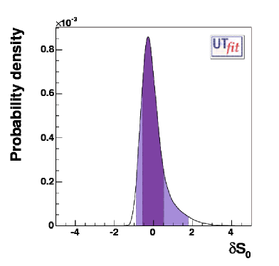
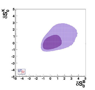
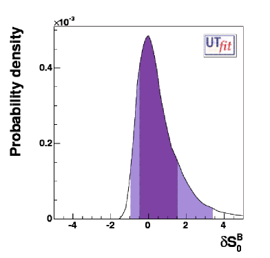
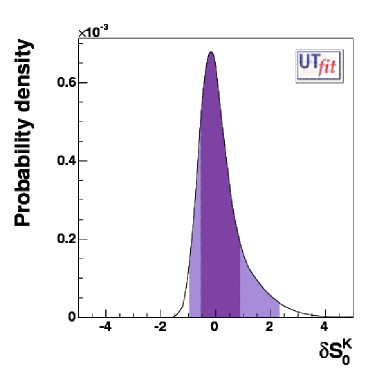
Figure 13: P.d.f. of $\delta S_{0}$ (top-left), $\delta S_{0}^{K}$ vs $\delta S_{0}^{B}$ (top-right), $\delta S_{0}^{B}$ (bottom-left) and $\delta S_{0}^{K}$ (bottom-right). See the text for details.

It is instructive to observe the two-dimensional plot of $\delta S_{0}^{B}$ vs. $\delta S_{0}^{K}$ in Fig. 13: within models with only one Higgs doublet or with small $\tan\beta$, the two $\delta$’s are bound to lie on the line $\delta S_{0}^{B}=\delta S_{0}^{K}$. The correlation coefficient $R$ provides a measure of this relation. We find $R=0.52$ giving no compelling indication on the value of $\tan\beta$.

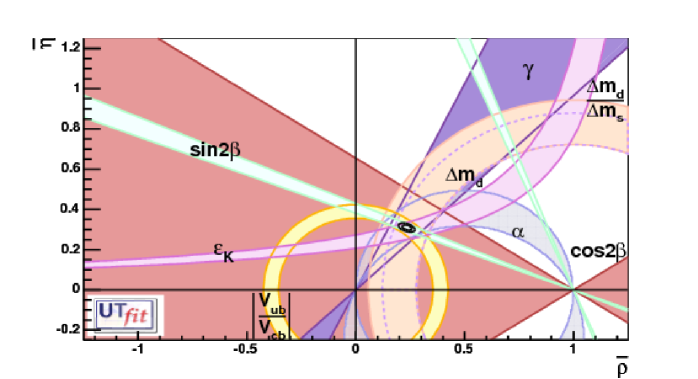
Figure 14: The selected region on $\bar{\rho}$-$\bar{\eta}$ plane obtained from the Standard Model UT analysis in the “year 2010” scenario.

6 Model Independent constraints on New Physics in the $\mathbf{|\Delta F|}$=2 sector in year 2010

Observable	projected value $\&$ error
$\sin 2\beta$	0.695 $\pm$ 0.010 (1.4$\%$)
$\alpha[^{\circ}]$	104 $\pm$ 5
$\gamma[^{\circ}]$ (DK)	54 $\pm$ 5
$B_{K}$	0.930 $\pm$ 0.047 (5$\%$)
$F_{B_{s}}\sqrt{\hat{B}_{B_{s}}}$ [MeV]	0.276 $\pm$ 0.014 (5$\%$)
$\xi$	1.200 $\pm$ 0.037 (3$\%$)
$\left|{V_{cb}}\right|$-(incl+excl) ($10^{-3}$)	41.7 $\pm$ 0.4 (0.9$\%$)
$\left|{V_{ub}}\right|$-(incl+excl) ($10^{-4}$)	36.4 $\pm$ 1.6 (4.2$\%$)
$\Delta m_{d}$ [ps-1]	0.503 $\pm$ 0.003 (0.6$\%$)
$m_{t}$ [GeV]	171 $\pm$ 3.0
$\lambda$	0.2240 $\pm$ 0.0008
$\Delta m_{s}$ [ps-1]	20.5 $\pm$ 0.3
$\sin 2\chi_{s}\,(J/\psi\phi)$	0.031 $\pm$ 0.045
$(\gamma-2\chi_{s})[^{\circ}]\,(D_{s}K)$	51 $\pm$ 10

Table 9: Projected values and errors in year 2010 for the most relevant quantities entering in the UT analysis. The central values are chosen such that the constraints are perfectly compatible within the SM.

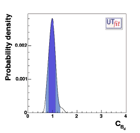
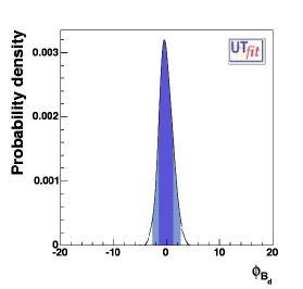
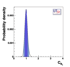
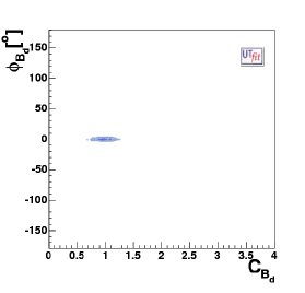
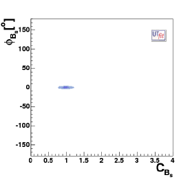
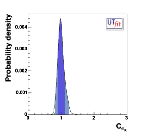
Figure 15: Projected situation in year 2010. p.d.f. distributions for NP parameters: from top to bottom and from left to right, distributions of $C_{B_{d}}$ and $\phi_{B_{d}}$, distributions of $C_{B_{s}}$ and $\phi_{B_{s}}$, 2D distributions of $\phi_{B_{d}}~{}vs.~{}C_{B_{d}}$ and $\phi_{B_{s}}~{}vs.~{}C_{B_{s}}$, and distribution of $C_{\epsilon_{K}}$. Dark (light) area corresponds to the $68\%$ ($95\%$) probability region.

We present an exercise on the knowledge of the UT parameters within the generalized NP analysis in a possible scenario in year 2010. At this date, the $B$ factories will have completed their data analysis and the LHCb experiment will have started running.

For this exercise we have assumed a total integrated luminosity for the $B$ factories of 2 ab^-1 and two years of data taking at LHCb, with an integrated luminosity of 4 fb^-1. At that time the lattice community will have produced the final numbers from the Tera-Flops machines. The 2010 projected values and errors for the quantities which are most relevant in UT analysis are given in Tab. 9. Lattice parameters are taken from [31], while the extrapolation of the errors on the experimental measurements is taken from [32, 33, 34, 35]. In addition to the improvements of existing measurements, we have added new measurements in the $B_{s}$ sector from LHCb. In particular the determination of

$\Delta m_{s}^{\mathrm{exp}}$	=	$C_{B_{s}}\Delta m_{s}^{\mathrm{SM}}$	$\mathrm{from}~{}B_{s}\to D_{s}\pi\,,$
$\sin 2\chi_{s}^{\mathrm{exp}}$	=	$\sin(2\chi_{s}^{\mathrm{SM}}+2\phi_{B_{s}})$	$\mathrm{from}~{}B_{s}\to J/\psi\phi\,,$
$(\gamma-2\chi_{s})^{\mathrm{exp}}$	=	$\gamma^{\mathrm{SM}}-2\chi_{s}^{\mathrm{SM}}-2\phi_{B_{s}}$	$\mathrm{from}~{}B_{s}\to D_{s}K\,.$

The central values for the different observables have been generated in the SM starting from an arbitrarily chosen value of $\bar{\rho}$ and $\bar{\eta}$, so that they are all compatible with each other and the result of the fit is fully “SM like”. The reason for this procedure is to investigate whether, in the “worst case” scenario of perfect confirmation of the SM, one can asymptotically reduce the errors on the NP related quantities introduced in the previous sections, and translate the derived constraint into a lower limit on the energy scale for NP particles. We start from a picture of what the UT analysis should look like in 2010. In Fig. 14 we show the selected region in the $\bar{\rho}$–$\bar{\eta}$ plane, while in the third column of Tab. 10 we quote the uncertainties on the various quantities from the UT analysis in the Standard Model. This should be taken as a reference for the approaches beyond the Standard Model that follow.

UT analysis in 2010
Observable	Input error	Output error
		SM UT	UUT
$\bar{\rho}$	-	0.015	0.021
$\bar{\eta}$	-	0.007	0.010
$\sin 2\beta$	0.010	0.009	0.009
$\alpha[^{\circ}]$	5	2.1	3.5
$\gamma[^{\circ}]$	5	2.0	3.2
$2\beta+\gamma[^{\circ}]$	-	2.3	3.4

Table 10: Projected uncertainties in year 2010 for the SM UT and the UUT analysis, using all the inputs of Tab. 9.

Moving from the SM analysis to the model independent approach of Sec. 3, we expect in the future a sizable improvement of the knowledge of the NP parameters:

$$C_{B_{d}}=0.98\pm 0.14\qquad \qquad\phi_{B_{d}}=(-0.1\pm 1.3)^{\circ}$$

$$C_{B_{s}}=0.99\pm 0.12\qquad \qquad\phi_{B_{s}}=(0.0\pm 1.3)^{\circ}$$

$$C_{\epsilon_{K}}=1.00\pm 0.10\qquad$$ (23)

as shown in Fig. 15.

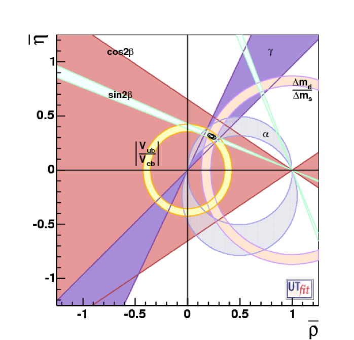
Figure 16: The selected region on $\bar{\rho}$-$\bar{\eta}$ plane obtained from the UUT analysis in the “year 2010” scenario.

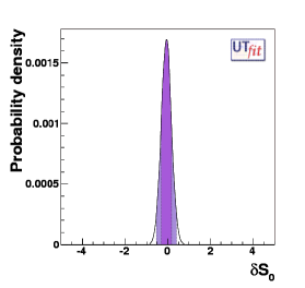
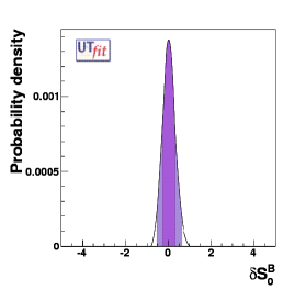
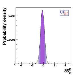
Figure 17: P.d.f. of $\delta S_{0}$ from MFV fit in the 2010 scenario, in the case of small (left) and large values of $\tan\beta$, from $B_{d,s}$–$\bar{B}_{d,s}$ (center) and $K$–$\bar{K}$ (right) mixing.

In the same future scenario, one can repeat the MFV analysis, both determining UT parameters using the UUT approach and adding the information from (NP sensitive) mixing quantities to bound the NP scale. The expected errors on the relevant UT quantities are summarized in the forth and fifth columns of Tab. 10.

If no evidence of violation of the Standard Model will emerge from $B$ physics in the era of direct NP search at LHC, this generalized approach will replace the present UT analysis as the default procedure. So, it is important to remark the fact that the generalization of the analysis costs an increasing of about $10\%$ of the errors, which is not a huge price to pay if compared to the gain in terms of the larger physics scenario. In Fig. 16, we give a hint of what the UUT analysis would look like in 2010.

In this framework, one should expect to increase the lower bound on $\Lambda$ when the NP sensitive quantities are added to the UUT fit. To have a quantitative example of the expected improvement, we used the input listed above for the 2010 scenario, obtaining the $\delta S_{0}$ distributions shown in Fig. 17. From these distributions, we get $\Lambda>7.5$($6.6$) TeV at $95\%$ probability, in the case of positive (negative) value of $\delta S_{0}$, in the case of MFV models with one Higgs doublet or low/moderate $\tan\beta$. For the case of large $\tan\beta$, we get

$$\Lambda > \left\{\begin{array}[]{l}6.0\mathrm{~{}TeV~{}@95\%~{}Prob.~{}for~{}positive~{}}\delta S_{0}^{B}\\ 6.6\mathrm{~{}TeV~{}@95\%~{}Prob.~{}for~{}negative~{}}\delta S_{0}^{B}\\ \end{array}\right.\mathrm{from~{}}B_{d,s}-\bar{B}_{d,s}\mathrm{~{}mixing}$$ (26)

$$\Lambda > \left\{\begin{array}[]{l}6.8\mathrm{~{}TeV~{}@95\%~{}Prob.~{}for~{}positive~{}}\delta S_{0}^{K}\\ 5.1\mathrm{~{}TeV~{}@95\%~{}Prob.~{}for~{}negative~{}}\delta S_{0}^{K}\\ \end{array}\right.\mathrm{from~{}}K-\bar{K}\mathrm{~{}mixing}$$ (29)

7 Conclusions

We have performed a model-independent analysis of the UT in general extensions of the SM with loop-mediated contributions to FCNC processes. Going beyond the pure tree-level determination of the UT already presented in Ref. [1], we have shown how the recent measurements performed at $B$ factories allow for a simultaneous determination of the CKM parameters together with the NP contributions to $|\Delta F|=2$ processes. We have found strong constraints on NP contributions that can be as large as the SM ones only if the SM and NP amplitudes have the same weak phase.

Motivated by this result, which points towards models with MFV, we have analyzed in detail the UUT. By putting together all the available information, it is possible to determine the UT parameters almost as accurately as in the SM case and to constrain the additional NP parameters. In this way, we probe dimension-six operators up to a scale of 5 TeV, to be compared with the SM reference scale of 2.4 TeV and to the sensitivity of other rare processes, which reaches scales of $9$–$12$ TeV in the case of $b\to s\gamma$ [6].

Finally, we have presented a possible scenario for the UT analysis in five years from now, taking into account foreseeable progress in theory and experiment, under the pessimistic assumption that the SM perfectly agrees with the data. This exercise allows us to assess the sensitivity to NP that we can expect in the near future. The impressive accuracy we can reach in this kind of analyses shows the great potential of flavour studies in investigating the structure of NP.

Note Added

While completing this work, we became aware of ref. [28], which contains an analysis similar to the one performed in Sec. 3.

References

- [1] M. Bona et al. [UTfit Collaboration], JHEP 0507 (2005) 028 [arXiv:hep-ph/0501199].
- [2] F. Gabbiani, E. Gabrielli, A. Masiero and L. Silvestrini, Nucl. Phys. B 477 (1996) 321 [arXiv:hep-ph/9604387].
- [3] L. J. Hall, V. A. Kostelecky and S. Raby, Nucl. Phys. B 267 (1986) 415.
- [4] A. Masiero, M. Piai, A. Romanino and L. Silvestrini, Phys. Rev. D 64 (2001) 075005 [arXiv:hep-ph/0104101].
- [5] A. J. Buras, P. Gambino, M. Gorbahn, S. Jager and L. Silvestrini, Phys. Lett. B 500 (2001) 161 [arXiv:hep-ph/0007085].
- [6] G. D’Ambrosio, G. F. Giudice, G. Isidori and A. Strumia, Nucl. Phys. B 645 (2002) 155 [arXiv:hep-ph/0207036].
- [7] A. J. Buras and R. Buras, Phys. Lett. B 501 (2001) 223 [arXiv:hep-ph/0008273]. A. J. Buras and R. Fleischer, Phys. Rev. D 64 (2001) 115010 [arXiv:hep-ph/0104238]. A. J. Buras, Phys. Lett. B 566 (2003) 115 [arXiv:hep-ph/0303060]. A. J. Buras, Acta Phys. Polon. B 34 (2003) 5615 [arXiv:hep-ph/0310208].
- [8] E. Gabrielli and G. F. Giudice, Nucl. Phys. B 433 (1995) 3 [Erratum-ibid. B 507 (1997) 549] [arXiv:hep-lat/9407029]. M. Misiak, S. Pokorski and J. Rosiek, Adv. Ser. Direct. High Energy Phys. 15 (1998) 795 [arXiv:hep-ph/9703442]. M. Ciuchini, G. Degrassi, P. Gambino and G. F. Giudice, Nucl. Phys. B 534 (1998) 3 [arXiv:hep-ph/9806308]. A. J. Buras, P. H. Chankowski, J. Rosiek and L. Slawianowska, Nucl. Phys. B 659 (2003) 3 [arXiv:hep-ph/0210145].
- [9] T. Appelquist, H. C. Cheng and B. A. Dobrescu, Phys. Rev. D 64 (2001) 035002 [arXiv:hep-ph/0012100]. A. J. Buras, M. Spranger and A. Weiler, Nucl. Phys. B 660 (2003) 225 [arXiv:hep-ph/0212143]. A. J. Buras, A. Poschenrieder, M. Spranger and A. Weiler, Nucl. Phys. B 678 (2004) 455 [arXiv:hep-ph/0306158].
- [10] C. Bobeth, M. Bona, A. J. Buras, T. Ewerth, M. Pierini, L. Silvestrini and A. Weiler, Nucl. Phys. B 726 (2005) 252 [arXiv:hep-ph/0505110].
- [11] M. Ciuchini, E. Franco, F. Parodi, V. Lubicz, L. Silvestrini and A. Stocchi, eConf C0304052 (2003) WG306 [arXiv:hep-ph/0307195].
- [12] M. Pierini in K. Hagiwara, J. Kanzaki and N. Okada, “Supersymmetry and unification of fundamental interactions. Proceedings, 12th International Conference, SUSY 2004, Tsukuba, Japan, June 17-23, 2004.”
- [13] S. Laplace, Z. Ligeti, Y. Nir and G. Perez, Phys. Rev. D 65 (2002) 094040 [arXiv:hep-ph/0202010].
- [14] Z. Ligeti, Int. J. Mod. Phys. A 20 (2005) 5105 [arXiv:hep-ph/0408267].
- [15] J. Charles et al. [CKMfitter Group], Eur. Phys. J. C 41 (2005) 1 [arXiv:hep-ph/0406184].
- [16] F. J. Botella, G. C. Branco, M. Nebot and M. N. Rebelo, Nucl. Phys. B 725 (2005) 155 [arXiv:hep-ph/0502133].
- [17] M. Ciuchini et al., JHEP 0107 (2001) 013 [arXiv:hep-ph/0012308].
-
[18]
Heavy Flavor Averaging Group,
http://www.slac.stanford.edu/xorg/hfag/index.html. - [19] A. Giri, Y. Grossman, A. Soffer and J. Zupan, Phys. Rev. D 68 (2003) 054018 [arXiv:hep-ph/0303187].
- [20] A. Amorim, M. G. Santos and J. P. Silva, Phys. Rev. D 59 (1999) 056001 [arXiv:hep-ph/9807364]. C. C. Meca and J. P. Silva, Phys. Rev. Lett. 81 (1998) 1377 [arXiv:hep-ph/9807320]. J. P. Silva and A. Soffer, Phys. Rev. D 61 (2000) 112001 [arXiv:hep-ph/9912242].
- [21] A. J. Buras, arXiv:hep-ph/0101336.
- [22] J. M. Soares and L. Wolfenstein, Phys. Rev. D 47 (1993) 1021. N. G. Deshpande, B. Dutta and S. Oh, Phys. Rev. Lett. 77 (1996) 4499 [arXiv:hep-ph/9608231]. J. P. Silva and L. Wolfenstein, Phys. Rev. D 55 (1997) 5331 [arXiv:hep-ph/9610208]. A. G. Cohen, D. B. Kaplan, F. Lepeintre and A. E. Nelson, Phys. Rev. Lett. 78 (1997) 2300 [arXiv:hep-ph/9610252]. Y. Grossman, Y. Nir and M. P. Worah, Phys. Lett. B 407 (1997) 307 [arXiv:hep-ph/9704287].
- [23] Y. Grossman and H. R. Quinn, Phys. Rev. D 56 (1997) 7259 [arXiv:hep-ph/9705356]. D. London, N. Sinha and R. Sinha, Phys. Rev. D 60 (1999) 074020 [arXiv:hep-ph/9905404]. F. J. Botella and J. P. Silva, Phys. Rev. D 71 (2005) 094008 [arXiv:hep-ph/0503136]. S. Baek, F. J. Botella, D. London and J. P. Silva, Phys. Rev. D 72 (2005) 036004 [arXiv:hep-ph/0506075].
- [24] M. Ciuchini, E. Franco, V. Lubicz, F. Mescia and C. Tarantino, JHEP 0308 (2003) 031 [arXiv:hep-ph/0308029].
- [25] D. Becirevic, V. Gimenez, G. Martinelli, M. Papinutto and J. Reyes, JHEP 0204 (2002) 025 [arXiv:hep-lat/0110091].
- [26] A. Bondar, T. Gershon and P. Krokovny, Phys. Lett. B 624 (2005) 1 [arXiv:hep-ph/0503174].
- [27] K. Abe et al., arXiv:hep-ex/0507065.
- [28] K. Agashe, M. Papucci, G. Perez and D. Pirjol, arXiv:hep-ph/0509117.
- [29] M. Ciuchini et al., JHEP 9810 (1998) 008 [arXiv:hep-ph/9808328].
- [30] D. Becirevic et al., Nucl. Phys. B 634 (2002) 105 [arXiv:hep-ph/0112303].
-
[31]
See the workshop Lattice QCD: Present and Future,
Orsay, April 14-16, 2004,
http://events.lal.in2p3.fr/conferences/lqcd/friday/lubicz.pdf,
http://events.lal.in2p3.fr/conferences/lqcd/friday/sharpe.pdf,
http://events.lal.in2p3.fr/conferences/lqcd/friday/giusti2.pdf. - [32] LHCb Collaboration, “LHCb technical design report: Reoptimized detector design and performance,” CERN-LHCC-2003-030
- [33] J. Hewett et al., arXiv:hep-ph/0503261.
-
[34]
D. Bernard et al., “Working Group : CP Violation and Heavy
Flavour” for Journees de perspectives DSM/DAPNIA-IN2P3,
http://prospective2004.in2p3.fr/textesdefinitifs/cp04final.ps. - [35] S. Amato et al. [LHCb Collaboration], CERN-LHCC-98-4