Lepton flavour violation in realistic non-minimal supergravity models
J. G. Hayes, S. F. King, I. N. R. Peddie 111Address after 1st September, 2005: Physics Division, School of Technology, Aristotle University of Thessaloniki, Thessaloniki 54124, Greece.
School of Physics and Astronomy, University of Southampton,
Southampton, SO17 1BJ, U.K.
Abstract
Realistic effective supergravity models have a variety of sources of lepton flavour violation (LFV) which can drastically affect the predictions relative to the scenarios usually considered in the literature based on minimal supergravity and the supersymmetric see-saw mechanism. We catalogue the additional sources of LFV which occur in realistic supergravity models including the effect of D-terms arising from an Abelian family symmetry, non-aligned trilinear contributions from scalar F-terms, as well as non-minimal supergravity contributions and the effect of different Yukawa textures. In order to quantify these effects, we investigate a string inspired effective supergravity model arising from intersecting D-branes supplemented by an additional family symmetry. In such theories the magnitude of the D-terms is predicted, and we calculate the branching ratios for and for different benchmark points designed to isolate the different non-minimal contributions. We find that the D-term contributions are generally dangerously large, but in certain cases such contributions can lead to a dramatic suppression of LFV rates, for example by cancelling the effect of the see-saw induced LFV in models with lop-sided textures. In the class of string models considered here we find the surprising result that the D-terms can sometimes serve to restore universality in the effective non-minimal supergravity theory.
1 Introduction
Lepton flavour violation (LFV) is a sensitive probe of new physics in supersymmetric (SUSY) models [1, 2]. In SUSY models, LFV arises due to off-diagonal elements in the slepton mass matrices in the ‘super-CKM’ (SCKM) basis, in which the quark and lepton mass matrices are diagonal [3]. In supergravity (SUGRA) mediated SUSY breaking the soft SUSY breaking masses are generated at the Planck scale, and the low energy soft masses relevant for physical proceses such as LFV are therefore subject to radiative corrections in running from the Planck scale to the weak scale. Off-diagonal slepton masses in the SCKM basis can arise both directly at the high energy scale (due to the effective SUGRA theory which is responsible for them), or can be radiatively generated by renormalisation group running from the Planck scale to the weak scale, for example due to Higgs triplets in GUTs or right-handed neutrinos in see-saw models which have masses intermediate between these two scales.
Neutrino experiments confirming the Large Mixing Angle (LMA) MSW solution to the solar neutrino problem [4] taken together with the atmospheric neutrino data [5] shows that neutrino masses are inevitable [6]. The presence of right-handed neutrinos, as required by the see-saw mechanism for generating neutrino masses, will lead inevitably to LFV, due to running effects, even in minimal SUGRA (mSUGRA) which has no LFV at the high energy GUT or Planck scale [7, 8]. Therefore, merely assuming SUSY and the see-saw mechanism, one expects LFV to be present. This has been studied, for example, in mSUGRA models with a natural neutrino mass hierarchy [9]. There is a large literature on the case of minimal LFV arising from mSUGRA and the see-saw mechanism [10].
Despite the fact that most realistic string models lead to a low energy effective non-minimal SUGRA theory, such theories have not been extensively studied in the literature, although a general analysis of flavour changing effects in the mass insertion approximation has recently been performed [11]. Such effective non-minimal SUGRA models predict non-universality of the soft masses at the high energy scale, dependent on the structure of the Yukawa matrices. Moreover there can be additional sources of LFV which also enter the analysis. For example, realistic effective SUGRA theories arising from string-inspired models will also typically involve some gauged family symmetry which can give an additional direct (as opposed to renormalisation group induced) source of LFV. This is because the D-term contribution to the scalar masses generated when the family symmetry spontaneously breaks adds different diagonal elements to each generation in the ‘theory’ basis, and generates non-zero off-diagonal elements in the SCKM basis, leading to LFV. This effect depends on the strength of the D-term contribution, which is expected to be close in size to the size of the uncorrected scalar masses. There can also be a significant contribution to non-universal trilinear soft masses leading to flavour violation [12, 13, 14] arising from the F-terms of scalars associated with the Yukawa couplings (for example the flavons of Froggatt-Nielsen theories).
The purpose of the present paper is to catalogue and quantitatively study the importance of all the different sources of LFV present in a general non-minimal SUGRA framework, including the effects of gauged family symmetry. Although the different effects have all been identified in the literature, there has not so far been a coherent and quantitative dedicated study of LFV processes, beyond the mass insertion approximation, which includes all these effects within a single framework. In order to quantify the importance of the different effects it is necessary to investigate these disparate souces of LFV numerically, both in isolation and in association with one another, within some particular SUGRA model. To be concrete we shall study the effective SUGRA models of the kind considered in [14] which have a sufficiently rich structure to enable all of the effects to be studied within a single framework. Within this class of models we shall consider specific benchmark points in order to illustrate the different effects. Some of these benchmark points were already previously considered in [14]. However in the previous study the important effect of D-terms arising from the Abelian family symmetry was not considered. Here we shall show that such D-terms are in fact calculable within the framework of the particular model considered, and can lead to significant enhancement (or suppression) of LFV rates, depending on the particular model considered.
The outline of this paper is as follows. In Section 2 we discuss soft supersymmetry breaking masses in supergravity. In Section 3 we summarise the flavour problem and catalogue the distinct sources of lepton flavour violation. In Section 4, we outline the aspects of the specific models that we shall study. In Section 5 we discuss the soft SUSY-breaking sector within this class of models, parameterise the F-terms, and write down the soft terms, including the D-term contribution to the scalar masses. We also discuss the D-terms associated with a family symmetry that are expected to lead to large lepton flavour violation. In Section 6 we specify two models in this class, define benchmark points and present the results of our numerical analysis of LFV for these benchmark points. Section 7 concludes the paper.
2 Soft terms from supergravity
We summarise here the standard way of getting soft SUSY breaking terms from supergravity. Supergravity is defined in terms of a Kähler function, , of chiral superfields (). Taking the view that supergravity arises as the low energy effective field theory limit of a string theory, the hidden sector fields are taken to correspond to closed string moduli states (), and the matter states are taken to correspond to open string states. In string theory, the ends of the open string states are believed to be constrained to lie on extended solitonic objects called .
Using natural units,
| (1) |
is the Kähler potential, a real function of chiral superfields. This may be expaned in powers of :
| (2) |
is the Kähler metric. is the superpotential, a holomorphic function of chiral superfields.
| (3) |
We expect the supersymmetry to be broken; if it is broken, then the auxilliary fields for some . As we lack a model of SUSY breaking, we introduce Goldstino angles as parameters that will enable us to explore different methods of breaking supersymmetry. We introduce a matrix, that canonically normalises the Kähler metric, 222 The subscripts on the Kähler potential means . However, the subscripts on the F-terms are just labels. [15]. We also introduce a column vector which satisfies . We are completely free to parameterise in any way which satisfies this constraint.
Then the un-normalised soft terms and trilinears appear in the soft SUGRA breaking potential [16]
| (4) |
The non-canonically normalised soft trilinears are then
| (5) | |||||
In this equation, it should be noted that the index runs over . However, by definition, the hidden sector part of the Kähler potential and the Kähler metrics is independent of the matter fields.
Assuming that the terms , the canonically normalised equation for the trilinear is
| (6) |
If the Yukawa hierarchy is taken to be generated by a Froggatt-Nielsen (FN) field, , such that , then we expect , and then , and so even though these fields are expected to have heavily sub-dominant F-terms, they contribute to the trilinears on an equal footing as the moduli.
If the Kähler metric is diagonal and non-canonical, then the canonically normalised scalar mass-squareds are given by
| (7) |
and the gaugino masses are given by
| (8) |
where is the ‘gauge kinetic function’. enumerates -branes in the model. In type I string models without twisted moduli these have the form .
Specifically, we use a Kähler potential that doesn’t have any twisted-moduli [17]:
| (9) | |||||
The notation is that the field theory scalars, the dilaton and the untwisted moduli originate from closed strings. Open string states are required to have their ends localised onto . The upper index then specifies which brane(s) their ends are located on, and if both ends are on the same brane, the lower index specifies which pair of compacitified extra dimensions the string is free to vibrate in.
3 Sources of lepton flavour violation
There are two parts to the flavour problem. The first is understanding the origin of the Yukawa couplings (and heavy Majorana masses for the see-saw mechanism), which lead to low energy quark and lepton mixing angles. In low energy SUSY, we also need to understand why flavour changing and/or CP violating processes induced by SUSY loops are so small. A theory of flavour must address both problems simultaneously. For a full discussion of this see the review [3].
There are two contributions that can lead to large amounts of flavour violation. The first is the non-alignment of the trilinear soft coupling matrices to the corresponding Yukawa matrices, due to the contribution , . The reasons why this can lead to large flavour violation are have been given before [14], where a numerical investigation of a model very similar to those considered herein finds that there is a large amount of flavour violation. The second contribution can come from scalar mass matrices which are not proportional to the identity in the theory basis, and lead to off-diagonal entries in the SCKM basis, resulting in flavour violation.
In this section we begin by defining the SCKM basis, and in the following subsections we systematically discuss a number of distinct sources of Lepton Flavour Violation (LFV) in SUGRA models. As well as considering generic SUGRA models, we also allow for a family symmetry, which easily lead to non-universal scalar mass matrices, and non-aligned trilinear matrices333By non-aligned trilinears, we mean that .
3.1 The SCKM Basis
The most convenient basis to work in for considering flavour violating decays, such as is the super-CKM (SCKM) basis, which is the basis where the Yukawa matrices are diagonal. If we define the unitary rotation matrices by
| (10) |
such that has positive eigenvalues. To convert the physical mass matrices to the SCKM basis, we rotate by the relevant matrix; for the left-handed scalar matrices and for the right-handed. Then flavour violation is proportional to the off-diagonal elements in the SCKM basis, and is suppressed by the diagonal values. The selectron mass matrix is 6 by 6, and the sneutrino mass matrix is 3 by 3 444The heavy right handed neutrinos cause the right-handed part of the sneutrino mass matrix to decouple by the electroweak scale.. The selectron mass matrix is
| (11) |
where . The sneutrino mass matrix is then
| (12) |
Off diagonal elements in any of the 3 by 3 submatrices in the SCKM basis will lead to flavour violation. We will now consider the block of . The arguments follow for any other block of or . The transformation to the SCKM basis is carried out by
| (13) |
is unitary, and is diagonal, so the first two terms will be diagonal. Any off-diagonality must come from the third term. If this is proportional to the identity at the GUT scale, it will be approximately equal to the identity at the electroweak scale, which is the scale we should be working at. The fact that this is only approximate is due to the presence of the right handed neutrino fields in the running of the soft scalar mass squared matrices. If, however, the soft mass squared matrices are not proportional to the identity at the GUT scale, then large off-diagonal values will be generated when rotating to the SCKM basis, unless the rotation happens to be small. Generally this won’t be the case. Since the family D-term contribution is not proportional to the identity555This statement assumes that the generational charges are not the same for both left- and right-handed fields. This would remove the point of the family symmetry generating the fermion mass hierarchy. this will usually be the case666One can, however, imagine some model with aberrant points in its parameter space where a non-universal non-zero D-term corrects a non-universal base mass matrix to give a universal net mass matrix. and so we expect large flavour violation in models with Abelian family symmetries when the D-terms correct the scalar mass matrices.
3.2 The relevance of the Yukawa textures
There is one subtlety concerning the size of the off-diagonal elements of the scalar mass matrices in the SCKM basis. This comes back to the definition of the SCKM basis as the basis in which the Yukawa matrices are diagonal. The larger the SCKM transformation between any ‘theory’ basis and the mass eigenstate basis for the Yukawa matrices, the larger the SCKM transformation that must be performed on the scalar mass matrices in going to the SCKM basis, hence the larger the off-diagonal elements of the scalar mass matrices in the SCKM basis generated from non-equal diagonal elements in the ‘theory’ basis. 777 Note that the D-terms make us sensitive to right-handed mixings in the Yukawa matrices, so the non-universal family charge structure for the right-handed scalar masses may lead to a non-universal generational hierarchy in the right-handed scalar mass matrices. The larger the off-diagonal entries in the SCKM basis compared to the diagonal ones, the greater will be the flavour violation. Also, the greater the mass difference between the diagonal elements in the ‘theory’ basis, the greater the size of the off-diagonal entries produced when rotating from the ’theory’ basis, hence the larger the flavour violating effect. Clearly these effects are sensitive to the size of the transformation required to go to the SCKM basis, which in turn is sensitive to the particular choice of Yukawa textures in the ‘theory’ basis. In this way, the choice of Yukawa texture can play an important part on controlling the magnitude of flavour violation, and we shall see examples of this later.
3.3 Running effects
Consider the case where, at the high-energy scale, the scalar mass matrices are proportional to the identity matrix and each soft trilinear coupling matrix is aligned to the corresponding Yukawa matrix:
| (14) |
This is often referred to as mSUGRA. In the quark sector, due to the quark flavour violation responsible for CKM mixing, when the scalar squark mass matrices are run down to the electroweak scale, they will run to non-universal scalar mass matrices and non-aligned trilinear coupling matrices. If this is the case, then in the SCKM basis, which is the basis where the Yukawa matrices are diagonal, off-diagonal elements in the scalar squark mass matrices or the trilinear squark mass matrices lead to flavour violation.
In the lepton sector, in the absence of neutrino masses the separate lepton flavour numbers are conserved and mSUGRA will not lead to any LFV induced by running the matrices down to low energy. However, in the presence of neutrino masses, with right-handed neutrino fields included to allow a see-saw explanation of neutrino masses and mixing angles, the separate lepton flavour numbers will be violated and, even in the mSUGRA type scenario, running effects will generate off-diagonal elements in the scalar mass matrices in the SCKM basis, resulting in low energy LFV.
3.4 Diagonal scalar mass matrices not propotional to the unit matrix
3.4.1 Non-minimal SUGRA
In non-minimal SUGRA the scalar mass matrices may be diagonal at the high-energy scale, but not proportional to the identity. In this case, there will be non-zero off-diagonal elements in the SCKM basis even with no contribution to running effects, or contribution from the trilinear coupling matrices.
One way of getting diagonal mass matrices not proportional to the unit matrix is from a SUGRA model corresponding to the low energy limit of a string model with D-branes. If each generation from the field theory viewpoint corresponds to a string attaching to different branes, then the masses predicted in the SUGRA can be different. This leads to diagonal but non-universal scalar mass matrices.
3.4.2 D-term contributions from broken family gauge groups
Another way of getting diagonal mass matrices not proportional to the unit matrix is by having a model with a gauge family symmetry, which is broken spontaneously. When the Higgs which breaks the family group, the flavon, gets a vev, it contributes a squark (slepton) mass contribution through the four point scalar gauge interaction which has two flavons and two squarks (sleptons).
To make the point more explicitly, consider a family group. Then the mass contribution is proportional to the charge under the family symmetry. As the point of a family symmetry is to explain the hierarchy of fermion masses, small quark mixing angles and large neutrino mixing angles, the charges are usually different.
Then, even if the mass matrix starts off as a universal matrix, it will be driven non-universal by the D-term contribution:
| (15) |
3.5 Non-aligned trilinears
3.5.1 Non-minimal SUGRA
One way of getting non-aligned trilinear matrices is by having the same sort of non-minimal SUGRA setup that leads to diagonal but non-universal mass matrices, as described in Section 3.4.1. From the supegravity equations from Section 2, the trilinears that appear in the soft Lagrangian, will be non-aligned if the trilinears predicted by the SUGRA model, are not democratic, i.e. if . From a string-inspired/SUGRA standpoint, if each generation is assigned to a different brane and extra-dimensional vibrational direction, then in general we expect to be different, due to the differing values of the Kähler metrics for the different brane assignents . When is transformed to the SCKM basis at the electroweak scale, there will then be large off-diagonal elements which contribute to flavour violating processes.
3.5.2 Flavon contributions from the Yukawa couplings
In general when one considers a family symmetry in order to understand the origin of the Yukawa couplings, the new fields arising from this can develop F-term vevs, and contribute to the supersymmetry breaking F-terms in a non-universal way. This leads to a dangerous source of flavour violating non-aligned trilinears: [12, 13, 14, 18],
| (16) |
where the Yukawa coupling in Eq. (16) arises from the an effective FN operator and is a polynomial of the FN field , , leading to
| (17) |
However the auxiliary field is proportional to the scalar component,
| (18) |
An example of this with an arbritary family symmetry is
| (19) |
The are arbiratry couplings, all of which should be for the symmetry to be considered natural. The are integers appearing as a power for the -th element of the above Yukawa, and it comprises the sum of the family charges for the th-generation left-handed field and th-generation right-handed field. In principle, if the Yukawa texture is set up so that each power is different, then each element in will be different from each other, and the physical trilinear matrix, will be non-aligned to the corresponding Yukawa. Due to the dependence on the charges of the different fields, this contribution to the trilinears is not diagonalised when we transform to the SCKM basis.
4 Intersecting D-brane models with an Abelian family symmetry
4.1 Symmetries and symmetry breaking
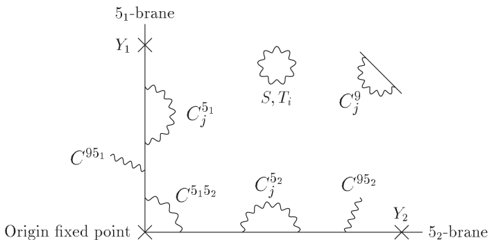
In order to study the effects of LFV elucidated in the previous section, it is necessary to specialize to a particular effective non-minimal SUGRA model which addresses the question of flavour (i.e. provides a theory of the Yukawa couplings). The specific model we shall discuss is defined in Table 1. This model is an extension of the Supersymmetric Pati-Salam model discussed in ref.[19], based on two branes which intersect at degrees and preserve SUSY down to the TeV energy scale. The generic D-brane set-up that we use is illustrated in Fig.1, where the string assignment notation is defined. The gauge group of the sector is , and the gauge group of the sector is (e.g., we assume the of the sector are broken). The symmetry breaking pattern of this model takes place in two stages, which we assume occur at very similar scales . In the first stage, the groups are broken to the diagonal subgroup via diagonal VEV’s of bifundamentals; the resulting theory is an effective Pati-Salam model (with additional ’s) which then breaks to the MSSM (and a number of additional ) via the usual Higgs pair of bifundamentals. The string scale is taken to be equal to the GUT scale, about GeV.
The symmetry breaking pattern leads to the following relations among the gauge couplings of the SM gauge groups in terms of the gauge couplings and associated with the gauge groups of the and sectors:
| (20) | |||||
| (21) | |||||
| (22) |
Field Ends charge 1 2 2 1 4 2 1 1 1 2 1 1 2 1 4 1 1 2 1 2 1 4 1 1 2 4 1 2 1 1 2 1 4 1 1 1 1 4 6 1 1 1 6 1 1 1 1 1 1 1 1 1 1 1 All
The extension is to include an additional family symmetry and the FN operators responsible for the Yukawa couplings as in [20] (see also [21]). The charges under the Abelian symmetry are left arbritary for now. The present ‘42241’ Model is the same as the model considered in [14], with the following modifications considered; firstly, we allow the Froggatt-Nielsen field to be either an intersection state or attached to the brane. The location of dramatically changes the value of the D-term contribution to the scalar masses coming from the FN sector.
The quark and lepton fields are contained in the representations which are assigned charges under . In Table 1 we list the charges, string assignments and representations under the string gauge group .
The field represents both Electroweak Higgs doublets that we are familiar with from the MSSM. The fields and are the Pati-Salam Higgs scalars;888We will also refer to these as “Heavy Higgs”; this has nothing to do with the MSSM heavy neutral higgs state . the bar on the second is used to note that it is in the conjugate representation compared to the unbarred field.
The extra Abelian gauge group is a family symmetry, and is broken at the high energy scale by the vevs of the FN fields [22] , which have charges and respectively under . We assume that the singlet field arises as an intersection state between the two , transforming under the remnant s in the 4224 gauge structure. In general the FN fields are expected to have non-zero F-term vevs.
The two gauge groups are broken to their diagonal subgroup at a high scale due to the assumed vevs of the bifundamental Higgs fields , [19]. The symmetry breaking at the scale
| (23) |
is achieved by the heavy Higgs fields , which are assumed to gain vevs [21]
| (24) |
This symmetry breaking splits the Higgs field into two Higgs doublets, , . Their neutral components then gain weak-scale vevs.
| (25) |
The low energy limit of this model contains the MSSM with right-handed neutrinos. We will return to the right handed neutrinos when we consider operators including the heavy Higgs fields , which lead to effective Yukawa contributions and effective Majorana mass matrices when the heavy Higgs fields gain vevs.
4.2 Yukawa operators
The (effective) Yukawa couplings are generated by operators involving the FN field with the following structure:999The field will not enter the Yukawa operators because will be positive for any . [21]:
| (26) |
where the integer is the total charge of and has a charge of zero. The tensor structure of the operators in Eq. (26) is
| (27) |
One constructs invariant tensors that combine and representations of into , , , and representations [21]. Similarly we construct tensors that combine the representations of into singlet and triplet representations. These tensors are contracted together and into to create singlets of , and . Depending on which operators are used, different Clebsch-Gordan coefficients (CGCs) will emerge.
We will return to these in section 6, when we define the two models that we will be using for the numerical analysis.
4.3 Majorana operators
We are interested in Majorana fermions because they can contribute neutrino masses of the correct order of magnitude via the see-saw effect. The operators for Majorana fermions are of the form
| (28) |
There do not exist renormalisable elements of this infinite series of operators, so Majorana operators are not defined, except in the element. We assume that a neturino mass term is allowed at leading (but non-renormalisable) order. A similar analysis goes through as for the Dirac fermions; however the structures only ever give masses to the neutrinos, not to the electrons or to the quarks.
5 Soft supersymmetry breaking masses
5.1 Supersymmetry breaking F-terms
In [19] it was assumed that the Yukawas were field-independent, and hence the only -vevs of importance were that of the dilaton (), and the untwisted moduli (). Here we set out the parameterisation for the F-term vevs, including the contributions from the FN field and the heavy Higgs fields . Note that the field dependent part follows from the assumption that the family symmetry field, is an intersection state.
| (29) | |||||
| (30) | |||||
| (31) | |||||
| (32) | |||||
| (33) |
We introduce a shorthand notation:
| (34) |
The F-terms above use values of and which are given in terms of the gauge couplings as:
| (35) |
The gauge couplings are given from Eq. (20)-(22) [19] as
| (36) |
where we shall assume that at the scale we have,
| (37) |
The values of are assumed to be equal and are obtained from the string relation
| (38) |
as
| (39) |
where we have taken
| (40) |
These rather small gauge couplings imply
| (41) |
In [14] the string relation was not used and it was assumed incorrectly that which resulted in .
5.2 Soft scalar masses
There are two contributions to scalar mass squared matrices, coming from SUGRA and from D-terms. In this subsection we calculate the SUGRA predictions for the matrices at the GUT scale, and in the next subsection we add on the D-term contributions.
The SUGRA contributions to soft masses are detailed in Section 2.
From Eq. (7) we can get the family independent form for all scalars:
| (45) | |||||
| (49) | |||||
| (50) | |||||
| (51) | |||||
| (52) | |||||
| (53) |
where
| (54) | |||||
| (55) | |||||
| (56) |
Here represents the left handed scalar mass squared matricies and . represents the right handed scalar mass squared matricies , , and . A discussion of the equations for can be found in Section 5.4.
5.3 D-term contributions
There are two D-term contributions to the scalar masses. The first is the well known [23, 14] contribution from the breaking of the Pati-Salam group to the MSSM group. Note that these D-terms are different to those quoted in the references above as we now consider the D-terms generated by breaking a family symmetry. See Appendix B for a full derivation. The second D-term comes solely from the breaking of the family symmetry. The corrections lead to the following mass matrices:
| (57) | |||||
| (58) | |||||
| (59) | |||||
| (60) | |||||
| (61) | |||||
| (62) | |||||
| (63) | |||||
| (64) |
The charges are the charges under of and respectively, as shown in Table 2. The correction factors are calculated explicitly in Appendix B in terms of the gauge couplings and soft masses as101010 is defined to be , thus for Model 1 and for Model 2. See Appendix B for more details.
| (65) | |||||
| (66) |
We note that the factors of appearing in the mass matrices are cancelled by the in the definition of .
The D-terms associated with the family symmetry depend on the charges of the left-handed and right-handed matter representations under the family symmetry. It is well known111111For an explanation, see for example [24]. that for Pati-Salam, one can choose any set of charges, and there will be an equivalent, shifted set of charges that are anomaly free due to the Green-Schwartz anomaly cancellation mechanism. The charges used for the D-term calculation should be the anomaly free charges.
The gauge couplings and mass parameters in Eqs. (65 , 66) are predicted from the model, in terms of the parameters and as shown in Eqs. (51 – 53) and Eqs. (68 – 70). Note that the D-terms will be zero if , or if the brane assignment is the same as . Choosing the second of these conditions is useful since it gives a comparison case where there are no D-terms; this comparison will make the D-term contribution to flavour violation immediately apparent.
5.4 Magnitude of -terms for different assignments
The main point worth emphasising is that in the string model the magnitudes of the -terms are calculable. We have assumed throughout that the FN field is an intersection string state , but have not specified the string assignment of . Thus takes various values depending on the string assignment for .
From Eq. (66), we see that we have calculable D-terms,
| (67) |
so the value of depends on the choice of where the field lives. We use Table 1 and Eqs. (45 - 56) to quantify the -term for each possible string assignment. As always lives at the intersection, on , our first choice of on is trivial: it gives . For on , is equivalent to , as this is also on . So using Eq. (50) for and Eq. (53) for in Eq. (67), we have
| (68) |
Similarly, the other two choices yield
| (69) | |||||
| (70) |
5.5 Soft gaugino masses
The soft gaugino masses are the same as in [19], which we quote here for completeness. The results follow from Eq. (8) applied to the gauginos, which then mix into the gauginos whose masses are given by
| (71) | |||||
| (72) | |||||
| (73) |
The values of and are proportional to the brane gauge couplings and , which are related in a simple way to the MSSM couplings at the unification scale. This is discussed in [19].
When we run the MSSM gauge couplings up and solve for and we find that approximate gauge coupling unification is achieved by . Then we find the simple approximate result
| (74) |
5.6 Soft trilinear couplings
So far we have considered the soft masses and the gaugino masses. The gaugino masses are the same as in [19]. The soft masses have had both D-term contributions added onto the base values from [19]. The contributions to the soft masses and gaugino masses from the FN and heavy Higgs auxiliary fields is completely negligible due to the small size of their F-terms. However for the soft trilinear masses these contributions are of order despite having small F-terms, so FN and Higgs contributions will give very important additional contributions beyond those considered in [19].
From Section 2 we see that the canonically normalised equation for the trilinear is
| (75) |
This general form for the trilinear accounts for contributions from non-moduli F-terms. These contributions are in general expected to be of the same magnitude as the moduli contributions despite the fact that the non-moduli F-terms are much smaller [25]. Specifically, if the Yukawa hierarchy is taken to be generated by a FN field, such that , then we expect , and then and so even though these fields are expected to have heavily sub-dominant F-terms121212In our model the FN and heavy Higgs vevs are of order the unification scale, compared to the moduli vevs which are of order of the Planck scale. they contribute to the trilinears at the same order as the moduli, but in a flavour off-diagonal way.
Here we sum over , which contains all the hidden sector fields: .
In the specific D-brane model of interest here, the general results for soft trilinear masses, including the contributions for general effective Yukawa couplings are given in Appendix A. From Eqs. (26, 27) we can read off the effective Yukawa couplings,
| (76) |
Note the extra group indices that the effective Yukawa coupling has, and proper care must be taken of the tensor structure when deriving trilinears from a given operator. We can write down the trilinear soft masses, , by substituting the operators in Eq. (C.1) into the results in Appendix A. Having done this we find the result:131313We assume that a Yukawa coupling appears at renormalisable order. This is why the doesn’t include contributions from and .
| (77) |
where
| (78) | |||||
| (79) | |||||
| (80) | |||||
| (81) | |||||
| (82) | |||||
| (83) |
These results are independent of which string assignment we give to , since this field does not enter the Yukawa operators.
6 Results
6.1 Two models
We will study two different models which have the same Yukawa textures, but different charge structures. The anomaly-free [24] family charges are laid out in Table 2. This first model is essentially the model studied in [20, 14], but with an extra operator in the and Yukawa matrix element to allow a non-zero and . The second model is defined such that all of the charges of left-handed matter are the same, causing the D-term to left handed scalar mass matrices to not lead to extra flavour violation. This choice is a small change to the model, since two of the ‘left-handed’ charges are the same anyway, and is made because normally the left-handed contribution dominates over the right-handed contribution. This can be achieved by changing the order of the operators in the Yukawa textures and the arbritary couplings to compensate the change in the charge structure, as discussed in Appendix C. Most of the results presented will be for Model 1.
Model 2 differs from Model 1 in the charges under the Abelian family symmetry, and the compensating changes to ensure the same Yukawa textues. As discussed in Appendix C there are two expansion parameters in these models which we take to be equal . The powers of in the first row of the Yukawa matrices are one lower, and we compensate that by increasing the powers of in the first row. We do not have to shift the values of the parameters since . Were this not the case, we would have to shift the values by a factor of . Model 2 is not meant to be a natural or realistic model, we use it as a tool to investigate the contribution to flavour violation from the D-term correction to the left-handed scalar masses. The family charges are laid out in Table 2.
The charge of must be equal and opposite to , and must be the negative of this. This is due to the (3,3) element of the right-handed Majorana mass being allowed at leading order, so the charges of and must conspire to cancel for the operator of the Majorana fermions to be renormalisable. For Model 1, the charges of and are and respectively. For Model 2, the charges of and are and respectively. One can use the relevent equations above to check that the anomaly coefficients do indeed satisfy the anomaly cancellation conditions. This gives us a different -term for Model 2, as indicated by in Eq. (65) being different for Model 1 and Model 2. Note that is the same in both models.
| Field | Model 1 | Model 2 |
| Charge | Charge | |
The values of the arbritary couplings are laid out in Appendix C in Table 4. This gives numerical values for the Yukawa elements which can be used in either model, with the relevant values of and inserted instead of the texture zeros:
| (87) | |||||
| (91) | |||||
| (95) | |||||
| (99) |
The RH Majorana neutrino mass matrix for Models 1 and 2 has the numerical values:
| (100) |
6.2 Benchmark points
Since the parameter space for the models is reasonably expansive, and the intention is to compare different sources of LFV, it is convenient to consider five benchmark points, as follows. It should be noted that for all these points, we have taken all to be the same, , and also . is taken to be zero throughout.
| Point | ||||||
|---|---|---|---|---|---|---|
| A | 0.500 | 0.500 | 0.000 | 0.000 | 0.000 | 0.000 |
| B | 0.535 | 0.488 | 0.000 | 0.000 | 0.000 | 0.000 |
| C | 0.270 | 0.270 | 0.000 | 0.000 | 0.841 | 0.000 |
| D | 0.270 | 0.270 | 0.595 | 0.595 | 0.000 | 0.000 |
| E | 0.290 | 0.264 | 0.000 | 0.000 | 0.841 | 0.000 |
-
•
Point A is referred to as “minimum flavour violation”. At the point the scalar mass matrices are proportional to the identity, and the trilinears are aligned with the Yukawas. Also, if we look back to Eqs. (65,66), (51) and (52), for , which is the case for point A (and points C and D) we see that the value of both D-term contributions is zero. As such, both and would be diagonal in the SCKM basis in the absence of the RH neutrino field, but in the presence of the see-saw mechanism off-diagonal elements are present in the SCKM basis leading to LFV. Since the four relevent soft masses are degenerate at this point, , both D-term contributions are zero; .
-
•
Point B is referred to as “SUGRA”. With it represents typical flavour violation from the moduli fields, manifested as diagonal soft mass matrices not proportional to the unit matrix in the theory basis; this is the amount of flavour violation that would traditionally have been expected with no contribution from the or fields. This and point E are the only benchmark points investigated where .
-
•
Point C is referred to as “FN flavour violation”. It represents flavour violation from the Froggatt-Nielsen sector by itself, arising as a non-alignment of the trilinear soft terms via the FN fields in the Yukawa operators, without any contribution to flavour violation from traditional SUGRA effects, since as in point A.
-
•
Point D is referred to as “Heavy Higgs flavour violation”. It represents flavour violation from the heavy Higgs sector, arising as a non-alignment of the trilinear soft terms, via the Heavy Higgs fields in the Yukawa operators, without any contribution from either traditional SUGRA effects since , or from FN fields since .
-
•
Point E combines features of points B and C, resulting in Froggatt-Nielsen flavour violation from , with SUGRA flavour violation from . This is the only point where we see the flavour violation from the Froggatt-Nielsen fields and the D-terms appearing at the same time. The numerical values for this point were obtained by taking the ratio from and for benchmark point B and applying it to benchmark point C.
6.3 Varying and
Normally, the chargino contribution to LFV dominates. Since the Feynman diagram for this includes the left-handed sfermions, we would expect the D-term corrections to the left-handed slepton mass matrix to dominate the flavour violation. However, Model 2, as defined in Section C.2, is set up to have universal left-handed charges, so the D-term correction from the breaking of will not contribute to flavour violation (except that it will either add or remove some mass suppression). The D-term is limited in magnitude by the difference of and , and although this is not a strong correction to the soft masses, it can contribute significantly to the lepton flavour violating branching ratios.
The difference in between Model 1 and Model 2 is negligible for . This should not be surprising, since the texture zero coming from will yield small mixing angles, resulting in small lepton flavour violation.
In order to get a picture of how great an effect the D-term contributions could have on the soft masses, it is necessary to examine a range of different values of and . An extra operator contribution was added to the textures in Model 1 and Model 2, when compared to the model previously studied [14], to allow for variations of the order , for example. The gives parameters and for Models 1 and 2 respectively. To be precise corresponds to and , and corresponds to .
6.4 Varying brane assignments for
The field is fixed to reside on the brane, but we allow the brane assignment of to vary over the possibilities , , and . This gives us D-terms that are calculable in each case, rather than being free parameters. The assignment of to , which is the same assigmment as the field, implies that the D-term calculated in this case is zero. The other possibilities, given in Eqs. (68 - 70), will highlight the contribution of the D-terms to lepton flavour violation.
6.5 Numerical procedure
The code used to generate all the data here was based on SOFTSUSY [28], which is a program that accurately calculates the spectrum of superparticles in the MSSM. It solves the renormalisation group equations with theoretical constraints on soft supersymmetry breaking terms provided by the user. Successful radiative electroweak symmetry breaking is used as a boundary condition, as are weak-scale gauge coupling and fermion mass data (including one-loop finite MSSM corrections). The program can also calculate a measure of fine-tuning. The program structure has, in this case, been adapted to the extension of the MSSM considered in this paper. It is modified to include right-handed neutrino fields, and thus non-zero neutrino masses and mixing angles, generated via the SUSY see-saw mechanism. It is also set up to include the new D-term contributions considered herein, and to run over a series of string assignments for the field. We use .
Electroweak symmetry breaking provides a significant constraint on the results. The breakdown of electroweak symmetry breaking was responsible for the ‘spike’ feature that was shown in the plots for benchmark points A and B in [14]. For the data above the spike, radiative electroweak symmetry breaking does not work properly, as the Z-boson mass becomes tachyonic. In the present paper such ‘bad’ regions where electroweak symmetry breaking fails are cut-off, however there is still a remnant of the spike left, which is why one can see a slight rise at the ends of the plots for our benchmark points A and B, as can be seen in Section 6.6.
6.6 Numerical results
We have now defined our two models, Model 1 and Model 2, and a set of five benchmark points in Table 3 to examine within them. We have also set up what we will be varying apart from the gravitino mass in these models – the values of , and the string assignment of which gives different D-terms. We are now in a position to present our results. We shall focus on the branching ratios for and . The branching ratio for is not shown here as it does not constrain us beyond those limits placed by and . The experimental limit for , at , is in fact far above the predicted rate for this process at all examined parts of the parameter space. In the following plots, we do not consider the assignment to as this is exactly the same as , due to the degeneracy of the . Were we to allow the to be non-degenerate, the phenomenological results of assigning to and would not be the same. The detailed spectrum will look different at each parameter point, but the general trend is for the physical masses to increase in magnitude as the gravitino mass increases. Thus too-high gravitino masses will start to reintroduce the fine-tuning problem resulting from the gluino mass being too high [29], although we shall not discuss the detailed spectrum here.
Figure 2 shows numerical results for for Model 1, plotted against the gravitino mass , where each of the four panels (i) – (iv) correspond to each of the four benchmark points A – D. 141414The solid line on each plot in Figure 2 corresponds to the solid lines in Figure 1 of [14]. However there were errors in the code used to generate the previous data, and the corrected rates shown here differ to the previous results by up to two orders of magnitude. Furthermore, unlike the results in [14], the results here do not exhibit a sharp spike for benchmark points A and B. For the data above the spike, radiative electroweak symmetry breaking does not work properly, as the Z-boson mass becomes tachyonic. This was not realized in the previous analysis. Panel (i) of Figure 2 refers to benchmark point A, corresponding to minimum flavour violation, where the only source of LFV is from the see-saw mechanism, which for Model 1 is well below the experimental limit, shown as the horizontal dot-dash line. Panel (ii) of Figure 2 refers to benchmark point B, with LFV arising from SUGRA, with the FN and heavy Higgs sources of LFV switched off. In this case one can clearly distinguish the additional contributions to LFV arising from the D-terms. This makes benchmark point B the most phenomenologically interesting for the purposes of this study. The differing contributions stem from the string assignments, which are shown by the separate lines: (solid), (dashed), and (dot-dash). The case shows the zero-D-term limit, where and are both intersection states, and hence conspire to cancel out via their soft masses being degenerate, . The other two locations for then turn on the -term contributions. With the D-terms switched on, Model 1 is experimentally ruled out over all parameter space shown here. Panel (iii) of Figure 2, refering to benchmark point C, is the Froggatt-Nielsen benchmark point, and for this case we see that the experimental limit is satisfied for over 1400 GeV. Panel (iv) of Figure 2, benchmark point D, shows the heavy Higgs point, for which the experimental limit is satisfied everywhere above 800 GeV. 151515Note that the predictions in this figure are lower than the corresponding figure in [14] due to the corrected values of , as discussed.
Figure 3 shows analogous results for for Model 1, plotted against the gravitino mass . All benchmark points come below the experimental limit for a substantial amount of the parameter space. The experimental limit here is more recent, and subsequently much more stringent than the previous limit. For these models in which there is a large (2,3) element in the neutrino Yukawa matrix the branching ratio for is essentially as constraining as that for , as first pointed out in [9]. The D-term coupling to right-handed scalars has a Yukawa mixing angle of order , compared to for . is the Wolfenstein parameter, which contributes on an equal footing to and . So the right-handed sector is of equal importance to the left-handed sector. We note that the see-saw effect enters prominently in the left-handed sector, and by considering Eqs. (57) and (58) for the soft scalar masses in the sector for , one can show that there is little effect coming from the D-terms coupling to left-handed scalars, since we have universal family charges for the left-handed sector, . For the right-handed scalars, however, the D-terms do play an important part and can have rather interesting and surprising effects, as we now discuss in some detail.
The solid line in panel (ii) of Figure 3 for the string assignment of has zero contribution from the D-terms, and shows just the effect of non-minimal SUGRA. This actually suppresses the flavour violation arising from the see-saw effect alone, showing an interesting cancellation between the LFV from the see-saw mechanism and the LFV from the non-universal D-terms. On the other hand the dashed line in panel (ii) for the case is very similar to the see-saw scenario of benchmark point A shown in panel (i). This is due to the D-terms actually conspiring to restore universality in the scalar masses, turning non-minimal SUGRA back into the minimal form. One can easily see this by applying Eq. (68) to Eqs. (59) - (62) for the right-handed scalar mass matrices, as the D-terms bring in an equal but opposite effect to the non-universal effects from SUGRA, and subsequently force the mass matrices to become universal. It is an amazing consequence of this string assignment for that in this model the effects of the non-universal D-terms can exactly cancel the effects of the non-universal SUGRA for the branching ratio of , leading to universal scalar mass matrices, even with SUGRA turned on. This is a string effect that directly affects the amount of flavour violation predicted in this scenario. For the case shown by the dot-dash line, applying Eq. (69) to the right-handed scalar mass matrices Eqs. (59) - (62) shows that the D-terms in this case actually enhance the effect of non-minimal SUGRA, causing the scalar mass matrices to become even more non-universal. One can understand this purely right-handed effect by considering the different mass insertion diagrams for the left- and right-handed sectors. The left-handed sector involves charginos, whereas the right-handed sector only involves neutralinos, so the right-handed masses scale differently with the gravitino mass as compared to the left-handed masses. Thus we do not have a universal mass scaling between the left- and right-handed sectors. This leads to the observed smooth cancellation of flavour violation between the two competing contributions from the see-saw mechanism and from SUGRA with additional D-terms.
Figure 4 shows benchmark point B for Model 1. The four panels show the and electron Yukawa elements being turned on and off. The results for Figure 4(i) are for and . This is the same as in panel (ii) of Figure 2, and is the base from which we start. Panel (ii) of Figure 4 has and , so we can clearly see the effect of turning on. It only affects the line, as the D-terms dominate over this effect for the other two string assignments. Panel (iii) of Figure 4 uses and , highlighting the effect of just alone. Again the zero D-term line of is the only one that is sizably affected by this change in Yukawa texture. Panel (iv) of Figure 4 shows the effect of turning on both Yukawa elements: and . We see that the shape of the solid line is determined by both Yukawa textures – they seem to have an equal impact on it.
Figure 5 shows benchmark point E, which combines the features of benchmark points B and C, thus both D-term and Froggatt-Nielsen (FN) flavour violation appear in the predicted branching ratios shown in this figure. There is some interesting interplay between the FN F-terms in the benchmark point C region of parameter space, and the D-terms in benchmark point B, and benchmark point E is designed to show this difference. In Figure 5 the results are shown for Model 1 with both and Yukawa elements on and off. The shape of the curves are as in benchmark point C due to being turned on, and the results are numerically similar to those of benchmark point C, showing that the dominant contribution comes from Froggatt-Nielsen flavour violation. However, as in benchmark point B, the different D-terms corresponding to different assignments leads to noticeable shifts in the results. In panel (i) with and it is seen that the presence of non-zero D-terms actually reduces the LFV rate somewhat compared to the solid curve with zero D-terms, corresponding to a region of parameter space where there is some cancellation between the flavour violation from the Froggat-Nielsen fields and that caused by the D-terms. The other panels show variation of the Yukawa elements as in Figure 4, for example panel (iv) corresponds to both and Yukawa elements being non-zero. Note that the solid curve in panel (iv) is slightly lower than the solid curve in panel (ii), showing that sometimes a non-zero Yukawa coupling can reduce LFV.
Figure 6 shows the effects of the Yukawa elements for benchmark point E using Model 2, where Model 2 has the same Yukawa structure as Model 1, but has the feature that the left-handed family charges are the same for all three families, resulting in universal D-terms, at least in the left-handed sector. Comparing Figure 6 to Figure 5, we see that in panel (i) of both figures with and there is no obserable difference between the predictions of the two models. However comparing panels (iv) of Figure 6 and Figure 5 we see that with non-zero and Model 2 has the effect of reducing the LFV resulting from the D-terms.
We could have presented similar plots for benchmark point D, with a new point F,161616The values for the parameters for benchmark point F would be which is an amalgamation of points B and D, but since this produces the same kind of results as Figure 5, we did not present the results.
7 Conclusions
We have catalogued and quantitatively studied the importance of all the different sources of LFV present in a general non-minimal SUGRA framework, including the effects of gauged family symmetry. We have discussed five different sources of LFV in such models: see-saw induced LFV arising from the running effects of right-handed neutrino fields; supergravity induced LFV due to the non-universal structure of the supergravity model; FN (Higgs) flavour violation, due to the F-terms associated with FN (Higgs) fields developing vevs, and contributing in a non-universal way to the soft trilinear terms; D-term flavour violation, where the D-term mass correction from the breaking of the Abelian family symmetry drives the scalar mass matrices to be non-universal; and finally the effects of different choices of Yukawa textures on LFV.
In order to quantify the importance of the different effects we investigated these disparate souces of LFV numerically, both in isolation and in association with one another, within a particular SUGRA model based on a type I string-inspired Pati-Salam model with an Abelian family symmetry, which has a sufficiently rich structure to enable all of the effects to studied within a single framework. Within this framework we derived the soft supersymmetry breaking terms, including the effect of the D-terms associated with breaking the family symmetry. For these models the D-terms are calculable, but are model dependent, depending on a particular choice of string assignment for the FN fields, and in particular the D-terms are only non-zero for the non-universal SUGRA models. We have performed a detailed numerical analysis of the five sources of LFV using five benchmark points designed to highlight the particular effects, and we have explored the effect of the variation of Yukawa texture elements on the results.
The most striking conclusion is how dangerously large the calculable D-term contribution to flavour violation can be, at least for the class of models studied. However it should be emphasised that while the D-terms are calculable in these models they are also model dependent, and it is always possible to simply switch off the D-terms by selecting the field to have the same string assignment as the intersection state. However other choices will lead to non-zero but calculable D-terms, which can be dangerously large, or can massively suppress flavour violation. For example the curves with non-zero D-terms in Figure 4 all exceed the experimental limit for the Branching Ratio for , showing that D-term effects have the potential to greatly exceed the other contributions from SUGRA, the see-saw mechanism, FN and Higgs, depending on the choice of Yukawa textures. However in some cases the D-terms generated by breaking the family symmetry can also suppress the Branching Ratio for , as shown in panels (i) and (iii) of Figures 5 and 6.
Another notable feature is the effect of Yukawa texture on the results. The Yukawa texture has , and we have shown that turning on non-zero values of these Yukawa couplings can greatly enhance the branching ratio for almost arbitarily. The reason is that the rotations to the SCKM basis are controlled by these Yukawa elements and the larger these rotations the larger will be the off-diagonal soft masses in the SCKM basis. The non-zero magnitudes of and were therefore chosen to be large enough to show the variations in the branching ratios of the different models, but small enough to keep within the currently experimentally allowed range.
In this paper we have worked with a particular Yukawa texture in which there is a large (2,3) element in the neutrino Yukawa matrix leading to large see-saw induced LFV and a branching ratio for which is as constraining as that for [9]. However we have seen that in some cases the D-terms can lead to a large suppression of the rate for particular values of , as seen in panel (ii) of Figure 3. For other cases the effects of the non-universal D-terms can exactly cancel the effects of the non-universal SUGRA model leading to universal scalar mass matrices, thereby restoring universality even for a non-minimal SUGRA model. Such effects are only possible in certain string set-ups and thus LFV provides an observable signal which may discriminate between different underlying string models.
In conclusion, we have seen that within realistic non-minimal supergravity models there can be several important effects leading to much larger LFV than in the case usually considered in the literature of minimum flavour violation corresponding to just mSUGRA and the see-saw mechanism, and considered here as benchmark point A. We find that the D-term contributions are generally dangerously large, but in certain cases such contributions can lead to a dramatic suppression of LFV rates, for example by cancelling the effect of the see-saw induced LFV in models with lop-sided textures. In the class of string models considered here we find the surprising result that the D-terms can sometimes serve to restore universality in the effective non-minimal supergravity theory. Thus D-terms can give very large and very surprising effects in LFV processes. In general there will be a panoply of different sources of LFV in realistic non-minimal SUGRA models, and we have explored the relative importance of some of them within a particular framework. The results here only serve to heighten the expectation that LFV processes such as and may be observed soon, although it is clear from our results that the precise theoretical interpretation of such signals will be more non-trivial than is apparent from many previous studies in the literature.
Acknowledgements
J.H. thanks PPARC for a studentship.
Appendix A Parameterised trilinears for the 42241 model
We here write the general form of the trilinear parameters assuming nothing about the form of the Yukawa matricies.
| (A.1) | |||||
| (A.2) | |||||
| (A.3) | |||||
| (A.4) | |||||
Appendix B Derivation of the D-terms
What follows is a full derivation of and from the superpotential of the extended supersymmetric Pati-Salam 42241 model, as detailed in Section 4.
The relevent parts of the superpotential for the 42241 model are those concerning the Higgs and Froggatt-Nielsen fields which have different gauge singlets171717Note that these must still have the same quantum numbers as they are both singlets, and therefore in the same representation of the gauge group..
| (B.1) |
where the and are GUT scale masses associated with the Higgs and Froggatt-Nielsen vevs respectively. We have assumed that the heavy Higgs develop vevs along the neutrino directions only, such that
| (B.2) |
This is because charged objects gaining vevs would break their charge group at the GUT scale, causing problems181818A colour charged object, for example, would imply that QCD is broken at the GUT scale, which would lead to a very massive gluon. which the neutral components avoid. Similarly, the Froggatt-Nielsen vevs are concisely written as
| (B.3) |
The F-terms associated with the singlet fields are
| (B.4) |
and
| (B.5) |
We use these to form our Higgs potential,
| (B.6) |
The F-term potential is trivially obtained from Eqs. (B.4) and (B.5), and the soft terms are simply written down with mass-squared terms for each of the soft SUSY-breaking scalar masses associated with the Higgs and FN vevs, as we will later see. The D-term potential takes a little more work, so we shall cover that here. The general form for the D-term potential is
| (B.7) |
where is the gauge coupling for , is for , and is for .
We focus on the and contributions to Eq. (B.7) which involve the
| (B.8) |
and
| (B.9) |
the diagonal generators of the and groups. There is no sum in the part of Eq. (B.7) because this group is the unit matrix 1, so the only generator is
| (B.10) |
where is the charge of the group for each field. When applying Eqs. (B.8) and (B.9) to conjugate fields we have to complex conjugate the generator and multiply it by , but for the group we just use Eq. (B.10) where it is known that the charges are different for right-handed fields.
Using Table 1 we find that , , and are given by
| (B.11) | |||||
| (B.12) | |||||
| (B.13) |
In Eq. (B.11), are family indices. We used to pick out the trace of the outer products and , thereby giving us the dot product.
The scalar components of the left-handed matter superfield are and . The scalar components of the right-handed matter superfield are , , , and . The tensorial conventions are shown in [23] for and . For , all diagonal elements are equal to unity for the generator, so the tensor notation is trivial.
Now we square , , and (as they are squared in the D-term potential), then consider the cross terms, as we are only interested in those terms that look like . The terms come from the vevs of the heavy Higgs and Froggatt-Nielsen fields . The terms come from , where the is a family index running from 1 to 3.
| (B.14) | |||||
| (B.15) |
where is defined to be and is defined to be , thus for Model 1 and for Model 2.
By considering the charge structure in Table 2 we can clearly see how the charge structure effects the additional D-term contributions to the sparticle mass matrices in Eqs. (57)-(64).
We have followed [23] in choosing our designation of , but is new. Working explicitly within Model 1, where , we shall proceed to rewrite these D-terms as functions of the soft SUSY breaking masses and gauge couplings. So we arrive at our D-term potential, which, when put together with and , forms our Higgs potential:
| (B.16) | |||||
where are the terms multiplied by gauge coupling factors, are the terms multiplied by the dilaton lambdas, and are the last four terms multiplying the TeV scale soft SUSY breaking scalar masses. and are GUT scale masses.
To find the form of the D-terms, we must minimise this potential with respect to the fields , , , , and then set these minimisation relations equal to zero.
As these are set to zero, any linear combination of them is also zero, so taking the following combinations and rearranging them, we have two minimisation conditions
| (B.17) | |||||
| (B.18) | |||||
For -flatness, it is necessary to set and , which results in . For -flatness and -flatness, it is necessary to set and , yielding zero valued F-terms. We wish to perturb away from these flatness conditions, so we impose
| ; | (B.19) | ||||
| ; | (B.20) |
where , , , and are all TeV scale masses.
Thus the two minimisation conditions, Eqs. (B.17) and (B.18), become191919After rearranging and taking the leading order in the GUT scale masses and .
| (B.21) | |||||
| (B.22) |
Now putting the small perturbations, Eqs. (B.19) and (B.20), into Eqs. (B.14) and (B.15) for the D-terms, we have, to leading order,
| (B.23) | |||||
| (B.24) |
So, using Eqs. (B.21) and (B.22) in the above Eqs. (B.23) and (B.24), we have the following expressions for our D-terms for Model 1, as functions of the soft SUSY breaking masses, GUT scale masses and gauge couplings
| (B.25) | |||||
| (B.26) |
Note that Eq. (B.26) was used in obtaining Eq. (B.25). This is the form of the D-terms as used in the updated version of SOFTSUSY [28] to compute the slepton mass data for our lepton flavour violating branching ratios in Model 1, using Eqs. (57) to (64).
For Model 2, the derivation is very similar, with the factor of being the only difference, and so we obtain the form of below, with being the same in both models.
| (B.27) |
In both cases, we can see that the Pati-Salam limit is obtained when the Froggatt-Nielsen scalar masses are degenerate, . This result differs from [23] due to a different derivation procedure.
Appendix C Operators for the two models
In this appendix we give the operators which are responsible for generating the Yukawa matrices of Models 1 and 2 analysed in this paper.
C.1 Model 1
| Model 1 | Model 2 | ||
|---|---|---|---|
| 0.22 | 0.22 | ||
| 0.22 | 0.22 | ||
| 0.55 | 0.55 | ||
| -0.92 | -0.92 | ||
| 0.33 | 0.33 | ||
| 0.00 | 0.00 | ||
| 1.67 | 1.67 | ||
| 1.12 | 1.12 | ||
| 0.89 | 0.89 | ||
| -0.21 | -0.21 | ||
| 2.08 | 2.08 | ||
| 0.77 | 0.77 | ||
| 0.53 | 0.53 | ||
| 0.66 | 0.66 | ||
| 0.40 | 0.40 | ||
| 1.80 | 1.80 | ||
| 0.278 | 0.278 | ||
| 0.000 | 0.000 | ||
| 0.000 | 0.000 | ||
| 0.94 | 0.94 | ||
| 0.48 | 0.48 | ||
| 2.10 | 2.10 | ||
| 0.52 | 0.52 | ||
| 1.29 | 1.29 | ||
| 1.88 | 1.88 | ||
This model is almost the model studied in [20, 14], but with an extra operator in the and Yukawa matrix elements to allow a non-zero and . The operator texture is
| (C.1) |
where the operator nomenclature is defined in Appendix D and Appendix E. This leads to the following Yukawa textures:
| (C.5) | |||||
| (C.9) | |||||
| (C.13) | |||||
| (C.17) |
For both models we define and as:
| (C.18) |
We take .
The values of the arbritary couplings are laid out in Table 4. This gives numerical values for the Yukawa elements which can be used in either model, with the relevant values of and inserted instead of the texture zeros:
| (C.22) | |||||
| (C.26) | |||||
| (C.30) | |||||
| (C.34) |
The RH Majorana neutrino mass matrix is:
| (C.35) |
The numerical values for the Majorana mass matrix are
| (C.36) |
C.2 Model 2
The operator texture for Model 2 is:
| (C.37) |
The operator nomenclature is defined in Appendix D and Appendix E. The new operator setup leads to the following Yukawa textures:
| (C.41) | |||||
| (C.45) | |||||
| (C.49) | |||||
| (C.53) |
The RH Majorana neutrino mass matrix is the same as in Model 1:
| (C.54) |
Appendix D operators
Operator Name Operator Name in [21]
The Dirac operators are the complete set of all operators that can be constructed from the quintilinear by all possible group theoretical contractions of the indicies in
| (D.1) |
We define some invariant tensors and some invariant tensors as follows202020The subscript denotes the dimension of the representation they can create from multiplying or with or . For example .:
| (D.2) |
Then the six independent structures are:
| (D.3) |
And the six structures are:
| (D.4) |
All possible operators were then named in [21]. We rename them here in a manner consistent with the operators , so that the names are where is the structure and is the SU2 structure. See Table 5 for the translation into the names of Ref.[21] and the CGCs.
All of these operators are operators for the case without a family symmetry. In the case when there is, we follow the prescription
| (D.5) |
Where is the modulus of the charge of the operator. If the charge of the operator is negative, then the field should be replaced by the field . The prescription makes the operator chargeless under the while simultaneously not changing the dimension.
Appendix E operators
In the case that , there will be more indicies to contract, which allows more representations, and hence more Clebsch coefficients. To generalise the notation, it is necessary only to construct the new tensors which create the new structures. However, it will always be possible to contract the new indicies between the and fields to create a singlet which has a Clebsch of 1 in each sector . In this case, the first structures are the same as the old structures, but with extra symbols which construct the singlet.
Thus taking an operator, say , which forms a representation that could have been attained by a operator, the Clebsch coefficients are the same. This is what we mean by , as we have only used coefficients which are in the subset that have analogues.
References
- [1] F. Borzumati and A. Masiero, Phys. Rev. Lett. 57 (1986) 961.
- [2] F. Gabbiani, E. Gabrielli, A. Masiero and L. Silvestrini, Nucl. Phys. B 477 (1996) 321 [arXiv:hep-ph/9604387].
- [3] D. J. H. Chung, L. L. Everett, G. L. Kane, S. F. King, J. Lykken and L. T. Wang, Phys. Rept. 407 (2005) 1 [arXiv:hep-ph/0312378].
- [4] G. L. Fogli, E. Lisi, A. Marrone, D. Montanino, A. Palazzo and A. M. Rotunno, arXiv:hep-ph/0212127; P. C. de Holanda and A. Y. Smirnov, arXiv:hep-ph/0212270; V. Barger and D. Marfatia, Phys. Lett. B 555 (2003) 144 [arXiv:hep-ph/0212126]; A. Bandyopadhyay, S. Choubey, R. Gandhi, S. Goswami and D. P. Roy, arXiv:hep-ph/0212146. M. Maltoni, T. Schwetz and J. W. Valle, arXiv:hep-ph/0212129.
- [5] Y. Fukuda et al., Super-Kamiokande Collaboration, Phys. Lett. B433, 9 (1998); ibid. Phys. Lett. B436, 33 (1998); ibid. Phys. Rev. Lett. 81, 1562 (1998).
- [6] For a review see: S. F. King, Rept. Prog. Phys. 67, 107 (2004) [arXiv:hep-ph/0310204].
- [7] J. Hisano, T. Moroi, K. Tobe and M. Yamaguchi, Phys. Rev. D 53 (1996) 2442 [arXiv:hep-ph/9510309].
- [8] S. F. King and M. Oliveira, Phys. Rev. D 60 (1999) 035003 [arXiv:hep-ph/9804283].
- [9] T. Blazek and S. F. King, arXiv:hep-ph/0211368.
- [10] S. Davidson and A. Ibarra, JHEP 0109 (2001) 013; J. Hisano and D. Nomura, Phys. Rev. D 59 (1999) 116005; J. Hisano, arXiv:hep-ph/0204100; J. A. Casas and A. Ibarra, Nucl. Phys. B 618 (2001) 171; W. Buchmüller, D. Delepine and F. Vissani, Phys. Lett. B 459 (1999) 171; M. E. Gomez, G. K. Leontaris, S. Lola and J. D. Vergados, Phys. Rev. D 59 (1999) 116009; J. R. Ellis, M. E. Gomez, G. K. Leontaris, S. Lola and D. V. Nanopoulos, Eur. Phys. J. C 14 (2000) 319; W. Buchmüller, D. Delepine and L. T. Handoko, Nucl. Phys. B 576 (2000) 445; D. Carvalho, J. Ellis, M. Gomez and S. Lola, Phys. Lett. B 515 (2001) 323; F. Deppisch, H. Pas, A. Redelbach, R. Ruckl and Y. Shimizu, arXiv:hep-ph/0206122; J. Sato and K. Tobe, Phys. Rev. D 63 (2001) 116010; J. Hisano and K. Tobe, Phys. Lett. B 510 (2001) 197; J. R. Ellis, J. Hisano, M. Raidal and Y. Shimizu, Phys. Lett. B 528 (2002) 86, arXiv:hep-ph/0111324; J. R. Ellis, J. Hisano, S. Lola and M. Raidal, Nucl. Phys. B 621 (2002) 208, arXiv:hep-ph/0109125; J. Hisano, T. Moroi, K. Tobe and M. Yamaguchi, Phys. Lett. B 391 (1997) 341; [Erratum - ibid. 397, 357 (1997)]; J. Hisano, D. Nomura, Y. Okada, Y. Shimizu and M. Tanaka, Phys. Rev. D 58 (1998) 116010; J. Hisano, D. Nomura and T. Yanagida, Phys. Lett. B 437 (1998) 351; S. Lavignac, I. Masina and C. A. Savoy, Phys. Lett. B 520 (2001) 269 [arXiv:hep-ph/0106245]; S. Lavignac, I. Masina and C. A. Savoy, Nucl. Phys. B 633 (2002) 139 [arXiv:hep-ph/0202086]; I. Masina and C. A. Savoy, arXiv:hep-ph/0211283. S. Pascoli, S. T. Petcov and C. E. Yaguna, Phys. Lett. B 564 (2003) 241 [arXiv:hep-ph/0301095]. S. Pascoli, S. T. Petcov and W. Rodejohann, arXiv:hep-ph/0302054.
- [11] P. H. Chankowski, O. Lebedev and S. Pokorski, Nucl. Phys. B 717 (2005) 190 [arXiv:hep-ph/0502076].
- [12] S. A. Abel and G. Servant, Nucl. Phys. B 611 (2001) 43 [arXiv:hep-ph/0105262].
- [13] G. G. Ross and O. Vives, Phys. Rev. D 67 (2003) 095013 [arXiv:hep-ph/0211279].
- [14] S. F. King, I. N. R. Peddie, Nucl. Phys. B 678 (2004) 339 [arXiv:hep-ph/0307091].
- [15] S. A. Abel, B. C. Allanach, F. Quevedo, L. Ibanez and M. Klein, JHEP 0012 (2000) 026 [arXiv:hep-ph/0005260]. B. C. Allanach, D. Grellscheid and F. Quevedo, JHEP 0205 (2002) 048 [arXiv:hep-ph/0111057].
- [16] A. Brignole, L. E. Ibanez and C. Munoz, [arXiv:hep-ph/9707209].
- [17] L. E. Ibanez, C. Munoz and S. Rigolin, Nucl. Phys. B 553 (1999) 43 [arXiv:hep-ph/9812397].
- [18] S. F. King and I. N. R. Peddie, J. Korean Phys. Soc. 45 (2004) S443 [arXiv:hep-ph/0312235].
- [19] L. L. Everett, G. L. Kane, S. F. King, S. Rigolin and L. T. Wang, Phys. Lett. B 531 (2002) 263 [arXiv:hep-ph/0202100].
- [20] T. Blazek, S. F. King and J. K. Parry, arXiv:hep-ph/0303192.
- [21] S. F. King, Phys. Lett. B 325 (1994) 129 [Erratum-ibid. B 325 (1994) 538]; B. C. Allanach and S. F. King, Nucl. Phys. B 456 (1995) 57 [arXiv:hep-ph/9502219]; B. C. Allanach and S. F. King, Nucl. Phys. B 459 (1996) 75 [arXiv:hep-ph/9509205]; B. C. Allanach, S. F. King, G. K. Leontaris and S. Lola, Phys. Rev. D 56 (1997) 2632 [arXiv:hep-ph/9610517]; S. F. King and M. Oliveira, Phys. Rev. D 63 (2001) 095004 [arXiv:hep-ph/0009287]
- [22] C. D. Froggatt and H. B. Nielsen, Nucl. Phys. B 147 (1979) 277.
- [23] S. F. King and M. Oliveira, Phys. Rev. D 63 (2001) 015010 [arXiv:hep-ph/0008183].
- [24] G. L. Kane, S. F. King, I. N. R. Peddie and L. Velasco-Sevilla, arXiv:hep-ph/0504038.
- [25] S. Abel, S. Khalil and O. Lebedev, Phys. Rev. Lett. 89 (2002) 121601 [arXiv:hep-ph/0112260].
- [26] K. Hagiwara et al. [Particle Data Group Collaboration], Phys. Rev. D 66 (2002) 010001.
- [27] B. Aubert et al. [BABAR Collaboration], Phys. Rev. Lett. 95 (2005) 041802 [arXiv:hep-ex/0502032].
- [28] B. C. Allanach, Comput. Phys. Commun. 143 (2002) 305 [arXiv:hep-ph/0104145].
- [29] G. L. Kane and S. F. King, Phys. Lett. B 451 (1999) 113 [arXiv:hep-ph/9810374].