Double Higgs Production and Quadratic Divergence Cancellation in Little Higgs Models with T-Parity

Abstract

We analyze double Higgs boson production at the Large Hadron Collider in the context of Little Higgs models. In double Higgs production, the diagrams involved are directly related to those that cause the cancellation of the quadratic divergence of the Higgs self-energy, providing a robust prediction for this class of models. We find that in extensions of this model with the inclusion of a so-called T-parity, there is a significant enhancement in the cross sections as compared to the Standard Model.

I Introduction

The presence of quadratic divergences in loop corrections to the scalar Higgs boson self-energy is responsible for the so-called hierarchy problem of the Standard Model (SM); namely, there is no natural way of having a “light” mass (i.e. $\sim 10^{2}$ GeV) for the Higgs given that loop corrections induce contributions to the mass of the order of the GUT scale –or in general the high energy scale above which new physics enters and the SM ceases to be an effective theory. In supersymmetric extensions of the SM this problem is absent since the bosons are protected from quadratic divergences by their relation to supersymmetric (fermion) partnerssusy1 . The hierarchy problem is also absent in models in which the electroweak symmetry is dynamically broken, since the scalar particles are not fundamental but composite in those cases techni2 .

Recently a new kind of model was proposed which can solve the hierarchy problem of the scalar Higgs boson. In these models, called Little Higgs (LH) models little3 , the Higgs boson is a pseudo-Goldstone boson and its mass is protected by a global symmetry and, unlike supersymmetry, quadratic divergence cancellations are due to contributions from new particles with the same spin.

The phenomenology of these models has been discussed with respect to indirect effects on precision measurements precision4 and direct production of the new particles introduced pheno5 .

Since these early contributions, several variations in the LH framework have been proposed review6 . However, the cancellation of quadratic divergences is inherent to any LH model and this requires definite relations among certain couplings. Therefore, any process that involves exclusively these couplings is a robust prediction of the LH mechanism regardless of model variations.

In this article we study a process that has ingrained in it the cancellation of quadratic divergences of top-quark loops, namely double Higgs production. In section II we review the model and the derivation of the masses and couplings of the relevant particles by appropriate diagonalization of mass matrices and show the cancellation of quadratic divergences directly in the broken symmetry phase. In section III we derive the amplitudes for double Higgs production at the Large Hadron Collider (LHC) and compute the cross sections. Our results are presented in section IV and we conclude in section V.

II Masses, couplings and quadratic divergences in the Littlest Higgs Model

There are many variations of Little Higgs models today, which differ in the symmetry groups and representations of the scalar multiplets, but they all have in common a mechanism of cancellation of the quadratic divergence for the mass of the lightest remaining scalars at one loop order. After the spontaneous breakdown of a global underlying symmetry at a scale $4\pi f$ (supposedly not much higher than a few TeV to avoid fine tuning), the model contains a large multiplet of pseudo-Goldstone bosons, which includes the SM Higgs doublet. While most members of the multiplet receive large masses (again, of a few TeV), the mass of the Higgs boson is protected from quadratic divergences at one loop, and therefore remains naturally smaller. The cancellation is related to the existence of an extra (heavier) top-like quark and its interactions with the scalar sector, feature which is common to all LH models. Consequently, a good test to distinguish a little Higgs from other cases should be based on a signal sensitive to this particular feature of divergence cancellation and rather insensitive to other features. The Higgs pair production at LHC is one of such signals, since it is based on exactly the same diagrams that enter the quadratic divergence cancellation (Fig. 1), except for the insertion of two gluons (Fig. 2 and 3).

In order to work out the details, we make use of the Littlest Higgs model, which is a simple case but contains all the necessary ingredients. After spontaneous breakdown of the (high-energy) underlying symmetry, the Little Higgs lagrangian below the scale $4\pi f$ littlest7 can be written as a non-linear sigma model based on a coset $SU(5)/SO(5)$ symmetry:

$${\cal L}_{\Sigma}=\frac{1}{2}\frac{f^{2}}{4}{\rm Tr}|{\cal D}_{\mu}\Sigma|^{2},$$ (1)

where the subgroup $[SU(2)\times U(1)]^{2}$ of $SU(5)$ is promoted to a local gauge symmetry. The covariant derivative is defined as

$${\cal D}_{\mu}\Sigma=\partial_{\mu}\Sigma-i\sum_{j=1}^{2}\left(g_{j}(W_{j}\Sigma+\Sigma W_{j}^{T})+g^{\prime}_{j}(B_{j}\Sigma+\Sigma B_{j}^{T})\right).$$ (2)

To exhibit the interactions, one can expand $\Sigma$ in powers of ${1}/{f}$ around its vacuum expectation value $\Sigma_{0}$

$$\Sigma=\Sigma_{0}+\frac{2i}{f}\left(\begin{array}[]{ccccc}\phi^{\dagger}&\frac{h^{\dagger}}{\sqrt{2}}&{\mathbf{0}}_{2\times 2}\\ \frac{h^{*}}{\sqrt{2}}&0&\frac{h}{\sqrt{2}}\\ {\mathbf{0}}_{2\times 2}&\frac{h^{T}}{\sqrt{2}}&\phi\end{array}\right)+{\cal O}\left(\frac{1}{f^{2}}\right),$$ (3)

where $h$ is the doublet that will remain light and $\phi$ is a triplet under the unbroken $SU(2)$. The non-zero vacuum expectation value of the field $\langle\Sigma\rangle=\Sigma_{0}$ leads to the breaking of the global $SU(5)$ symmetry to $SO(5)$ and also breaks the local gauge symmetry $[SU(2)\times U(1)]^{2}$ into its diagonal subgroup, which is identified with the standard model $SU_{L}(2)\times U_{Y}(1)$ symmetry group. Following the notation of Han et al. pheno5 , we will denote the usual standard model gauge bosons mass eigenstates as $W^{\pm}_{L}$, $Z_{L}$ and $A_{L}$, where the subscript $L$ denotes light in order to distinguish from the heavy states with mass of order $f$, denoted by $W^{\pm}_{H}$, $Z_{H}$ and $A_{H}$.

The standard model fermions acquire their masses via the usual Yukawa interactions. However, in order to cancel the top quark quadratic contribution to the Higgs self-energy, a new-vector like color triplet fermion pair, $\tilde{t}$ and $\tilde{t}^{\prime c}$, with quantum numbers $({\mathbf{3,1}})_{Y_{i}}$ and $({\mathbf{\bar{3},1}})_{-Y_{i}}$ must be introduced. Since they are vector-like, they are allowed to have a bare mass term which is chosen such as to cancel the quadratic divergence above scale $f$.

The coupling of the standard model top quark to the pseudo-Goldstone bosons and the heavy colored fermions in the littlest Higgs model is chosen to be

$${\cal{L}}_{Y}=\frac{1}{2}\lambda_{1}f\epsilon_{ijk}\epsilon_{xy}\chi_{i}\Sigma_{jx}\Sigma_{ky}u^{\prime c}_{3}+\lambda_{2}f\tilde{t}\tilde{t}^{\prime c}+{\rm h.c.},$$ (4)

where $\chi_{i}=(b_{3},t_{3},\tilde{t})$ and $\epsilon_{ijk}$ and $\epsilon_{xy}$ are antisymmetric tensors. The new model parameters $\lambda_{1},\ \lambda_{2}$ are supposed to be of the order

of unity.

The linearized part of Eq. 4 describing the third generation mass terms and interactions with the neutral Higgs field, denoted by $h^{0}$, (before spontaneous symmetry breaking, SSB), is given by:

$${\cal L}_{t}=\lambda_{2}f\tilde{t}\tilde{t}^{\prime c}-i\lambda_{1}\sqrt{2}t_{3}h^{0}u_{3}^{\prime c}+\lambda_{1}f\tilde{t}u_{3}^{\prime c}-\frac{\lambda_{1}}{f}\tilde{t}h^{0}h^{0\ast}u_{3}^{\prime c}+h.c.$$ (5)

After SSB, we write $h^{0}=1/\sqrt{2}(v+H)$, and follow Perelstein et al. PPP8 in defining left handed fields $t_{3L}\equiv t_{3}$, $\tilde{t}_{L}\equiv\tilde{t}$ and right handed fields $\bar{u}_{3R}^{\prime}\equiv u_{3}^{\prime c}$, $\bar{\tilde{t}}^{\prime}_{R}\equiv\tilde{t}^{\prime c}$ to obtain

$${\cal L}_{t} = \left(\begin{array}[]{cc}\bar{u}_{3R}^{\prime}&\bar{\tilde{t}}^{\prime}_{R}\end{array}\right)\left(\begin{array}[]{cc}-i\lambda_{1}v&\lambda_{1}f(1-v^{2}/2f^{2})\\ 0&\lambda_{2}f\end{array}\right)\left(\begin{array}[]{c}t_{3L}\\ \tilde{t}_{L}\end{array}\right)-i\lambda_{1}H\bar{u}_{3R}^{\prime}t_{3L}$$

$$-\lambda_{1}\frac{v}{f}H\bar{u}_{3R}^{\prime}\tilde{t}_{L}-\frac{\lambda_{1}}{2f}H^{2}\bar{u}_{3R}^{\prime}\tilde{t}_{L}+h.c.$$

In order to leave the fermion mass term in its standard form we make the field redefinitions $t_{3L}\rightarrow-it_{3L}$ and $\tilde{t}_{L}\rightarrow-\tilde{t}_{L}$ in the left-handed fields resulting in the following lagrangian:

$${\cal L}_{t} = -\left(\begin{array}[]{cc}\bar{u}_{3R}^{\prime}&\bar{\tilde{t}}^{\prime}_{R}\end{array}\right)\left(\begin{array}[]{cc}\lambda_{1}v&\lambda_{1}f(1-v^{2}/2f^{2})\\ 0&\lambda_{2}f\end{array}\right)\left(\begin{array}[]{c}t_{3L}\\ \tilde{t}_{L}\end{array}\right)-\lambda_{1}H\bar{u}_{3R}^{\prime}t_{3L}$$

$$+\lambda_{1}\frac{v}{f}H\bar{u}_{3R}^{\prime}\tilde{t}_{L}+\frac{\lambda_{1}}{2f}H^{2}\bar{u}_{3R}^{\prime}\tilde{t}_{L}+h.c.$$

Diagonalizing the mass matrix

$$M=\left(\begin{array}[]{cc}\lambda_{1}v&\lambda_{1}f(1-v^{2}/2f^{2})\\ 0&\lambda_{2}f\end{array}\right)$$ (18)

we obtain the usual result for the eigenvalues corresponding to the top quark $t$ and the heavy top $T$ which are, up to order ${\cal O}(v/f)$:

$$m_{t}=\frac{\lambda_{1}\lambda_{2}}{\sqrt{\lambda_{1}^{2}+\lambda_{2}^{2}}}\;v\;;\;\;\;m_{T}=\sqrt{\lambda_{1}^{2}+\lambda_{2}^{2}}\;f.$$ (19)

In our numerical code, we will use as input the values of $m_{T}$ and $f$, from which one obtains the required values of $\lambda_{1}$ and $\lambda_{2}$:

$$\lambda_{1(2)}^{2}=\frac{m_{T}^{2}}{2f^{2}}\left(1+(-)\sqrt{1-4\frac{m_{t}^{2}f^{2}}{v^{2}m_{T}^{2}}}\right).$$ (20)

From equation (20), one clearly sees that there is a condition relating top masses and v.e.v.’s that these models impose:

$$m_{T}>2\frac{m_{t}{}v}{f}\simeq\sqrt{2}f$$ (21)

and which we incorporate in our analysis. The relevant couplings between Higgs and top quarks are obtained in a straightforward manner after diagonalization of Eq. II and are given by (the corresponding vertices are obtained via multiplication by $(-i)$):

$$g_{Htt} = \frac{\lambda_{1}\lambda_{2}}{\sqrt{\lambda_{1}^{2}+\lambda_{2}^{2}}}$$ (22)

$$g_{HT_{R}t_{L}} = \frac{\lambda_{1}^{2}}{\sqrt{\lambda_{1}^{2}+\lambda_{2}^{2}}}$$

$$g_{HTT} = -\frac{\lambda_{1}^{2}\lambda_{2}^{2}}{(\lambda_{1}^{2}+\lambda_{2}^{2})^{3/2}}\;\frac{v}{f}$$

$$g_{HHTT} = -\frac{1}{f}\frac{\lambda_{1}^{2}}{\sqrt{\lambda_{1}^{2}+\lambda_{2}^{2}}}$$

$$g_{HHtt} = \frac{m_{t}}{f^{2}}\frac{\lambda_{1}^{2}}{\lambda_{1}^{2}+\lambda_{2}^{2}-4fv^{\prime}/v^{2}}$$

$$g_{Ht_{R}T_{L}} = -\frac{\lambda_{1}\lambda_{2}^{3}}{(\lambda_{1}^{2}+\lambda_{2}^{2})^{3/2}}\;\frac{v}{f}$$

The relevant Feynman diagrams for the Higgs self-energy are shown in figure (1).

Figure 1: One-loop corrections to the Higgs mass, to order $v/f$: (a) standard top quark loop, (b) mixture of standard and extra top quark loop, (c) extra top quark loop with a 4-particle vertex, and (d) tadpoles with standard and with extra top quark loops. There are other diagrams but they are suppressed by factors of order $(v/f)^{2}$ or higher.

The cancellation of tadpole diagrams requires that

$$g_{Htt}m_{t}+g_{HTT}m_{T}=0$$ (23)

whereas the cancellation of higgs self-energy quadratic divergences implies

$$g_{Htt}^{2}+g_{HTT}^{2}+g_{HT_{R}t_{L}}^{2}+g_{Ht_{R}T_{L}}^{2}+g_{HHtt}\;m_{t}+g_{HHTT}\;m_{T}=0$$ (24)

These conditions are satisfied up to terms of order ${\cal O}(v/f)$ by the masses and couplings listed above.discrepancy89

In the simplest LH models, strict bounds on the parameters are obtained. In particular, electroweak precision constraints require $f>3.5$ TeV precision4 . However, in a recent variation on the littlest Higgs model, where a so-called T-parity that interchanges the two subgroups $[SU(2)\times U(1)]_{1}$ and $[SU(2)\times U(1)]_{2}$ of $SU(5)$ is introduced, can significantly lower this bound to $f>500$ GeV TParity9 . This is an important point for the phenomenology of these models, since a lower $f$ implies larger deviations from the SM. Since the T-odd states do not participate in the cancellation of quadratic divergences, our calculation is valid in models with T-parity as well. T-parity also forbids the generation of a vacuum expectation value for the triplet scalar field (i.e., $v^{\prime}=0$ in the notation of T. Han et al.pheno5 ), which is one of the causes for easing the electroweak constraints.

III Amplitudes for double Higgs production

We now turn to Higgs boson production at the LHC in the LH model, which involves the very same couplings responsible for the cancellation of quadratic divergences.

Gluon-gluon fusion is the dominant mechanism for SM Higgs boson pair production at the LHC dhiggs10 . The amplitude for $gg\rightarrow HH$ is dominated by top quark loops, in the form of triangle and box diagrams. Figs. 2 and 3 show the case for a LH model. The SM case is similar, except that Fig. 2.a and all extra heavy-top loops are absent. We also would like to point out that T-parity forbids a term like $hh\phi$ in the radiatively generated Coleman-Weinberg potential. Therefore, there is no contribution of the heavy scalar in Fig. 2.b and the trilinear Higgs coupling is the same as in the SM.

Figure 2: Triangle contributions to Higgs boson pair production at LHC in a Little Higgs model.

Figure 3: Box contributions to Higgs boson pair production at LHC in a Little Higgs model.

Let us now write the expressions for the amplitude. In what follows, the external momenta $p_{a}$, $p_{b}$, $p_{c}$, $p_{d}$ are defined as incoming. The contribution from triangle diagrams is given by:

$$i{\cal M}^{\triangle}(g_{a}g_{b}\rightarrow H_{c}H_{d}) = -\frac{\alpha_{s}}{4\pi^{3}}\delta_{AB}\left(g_{Htt}I(m_{t})\frac{g_{HHH}}{\hat{s}-M_{H}^{2}-iM_{H}\Gamma_{H}}\right.$$

$$\left.+\,g_{HTT}I(m_{T})\frac{g_{HHH}}{\hat{s}-M_{H}^{2}-iM_{H}\Gamma_{H}}+g_{HHtt}I(m_{t})+g_{HHTT}I(m_{T})\right)$$

where the integral $I(m_{Q})$ is:

$$I(m_{Q})=\int d^{4}q\;\frac{Tr\left[(\hbox to0.0pt{/\hss}q+m_{Q})\gamma^{\mu}(\hbox to0.0pt{/\hss}q+\hbox to0.0pt{/\hss}p_{a}+m_{Q})\gamma^{\nu}(\hbox to0.0pt{/\hss}q+\hbox to0.0pt{/\hss}p_{a}+\hbox to0.0pt{/\hss}p_{b}+m_{Q})\right]}{[q^{2}-m_{Q}^{2}][(q+p_{a})^{2}-m_{Q}^{2}][(q+p_{a}+p_{b})^{2}-m_{Q}^{2}]}\epsilon_{\mu}(p_{a})\epsilon_{\nu}(p_{b}).$$ (26)

This integral reduces to the following result:

$$I(m_{Q})=i\;4\pi^{2}\;m_{Q}[1+(2m_{Q}^{2}-\hat{s}/2)C_{0}(0,0,\hat{s},m_{Q}^{2},m_{Q}^{2},m_{Q}^{2})]\epsilon(p_{a})\cdot\epsilon(p_{b}),$$ (27)

where $C_{0}$ is the scalar Passarino-Veltman integralPassarino defined as:

$$C_{0}=\int\frac{d^{4}q}{i\pi^{2}}\;\frac{1}{[q^{2}-m_{Q}^{2}][(q+p_{a})^{2}-m_{Q}^{2}][(q+p_{a}+p_{b})^{2}-m_{Q}^{2}]}$$ (28)

The contribution from box diagrams can be written as:

$$i{\cal M}^{\Box}(g_{a}g_{b}\rightarrow H_{c}H_{d}) = -\frac{\alpha_{s}}{8\pi^{3}}\delta_{AB}\left(g_{Htt}^{2}I_{1}(m_{t})+g_{HTT}^{2}I_{1}(m_{T})+I_{2}(m_{t},m_{T})\right)$$ (29)

Because the Higgs vertex is not diagonal in the $(t,T)$ flavor, there are two types of boxes. The function $I_{1}$ comes from boxes with either only standard top quarks or only extra heavy-top quarks in them, whereas the function $I_{2}$ comes from boxes with both tops and extra heavy-tops.

There are two basic box diagrams, planar (Fig. 3.a) and non-planar (Fig.3.b), according to whether the Higgses are adjacent in the loop or not. A planar box with a single type of quark is given by:

$$I^{P}_{1}(m_{Q}) = \int d^{4}q\;\frac{Tr\left[(\hbox to0.0pt{/\hss}q+m_{Q})\gamma^{\mu}(\hbox to0.0pt{/\hss}q+\hbox to0.0pt{/\hss}p_{a}+m_{Q})\gamma^{\nu}(\hbox to0.0pt{/\hss}q+\hbox to0.0pt{/\hss}p_{a}+\hbox to0.0pt{/\hss}p_{b}+m_{Q})(\hbox to0.0pt{/\hss}q+\hbox to0.0pt{/\hss}p_{a}+\hbox to0.0pt{/\hss}p_{b}+\hbox to0.0pt{/\hss}p_{c}+m_{Q})\right]}{[q^{2}-m_{Q}^{2}][(q+p_{a})^{2}-m_{Q}^{2}][(q+p_{a}+p_{b})^{2}-m_{Q}^{2}][(q+p_{a}+p_{b}+p_{c})^{2}-m_{Q}^{2}]}$$ (30)

$$\times\epsilon_{\mu}(p_{a})\epsilon_{\nu}(p_{b})\quad+\,\Big{\{}p_{a}\leftrightarrow p_{b}\Big{\}}\,+\,\Big{\{}p_{c}\leftrightarrow p_{d}\Big{\}}\,+\,\Big{\{}p_{a}\leftrightarrow p_{b},\,p_{c}\leftrightarrow p_{d}\Big{\}},$$

while a non-planar box is:

$$I^{NP}_{1}(m_{Q}) = \int d^{4}q\;\frac{Tr\left[(\hbox to0.0pt{/\hss}q+m_{Q})\gamma^{\mu}(\hbox to0.0pt{/\hss}q+\hbox to0.0pt{/\hss}p_{a}+m_{Q})(\hbox to0.0pt{/\hss}q+\hbox to0.0pt{/\hss}p_{a}+\hbox to0.0pt{/\hss}p_{c}+m_{Q})\gamma^{\nu}(\hbox to0.0pt{/\hss}q+\hbox to0.0pt{/\hss}p_{a}+\hbox to0.0pt{/\hss}p_{b}+\hbox to0.0pt{/\hss}p_{c}+m_{Q})\right]}{[q^{2}-m_{Q}^{2}][(q+p_{a})^{2}-m_{Q}^{2}][(q+p_{a}+p_{c})^{2}-m_{Q}^{2}][(q+p_{a}+p_{b}+p_{c})^{2}-m_{Q}^{2}]}$$ (31)

$$\times\epsilon_{\mu}(p_{a})\epsilon_{\nu}(p_{b})\quad+\,\Big{\{}p_{a}\leftrightarrow p_{b}\Big{\}}$$

The total contribution for boxes with a single type of quark is then

$$I_{1}(m)=I^{P}(m)+I^{NP}(m)$$ (32)

We also have to compute the contribution of box diagrams with both $t$ and $T$ running in the loop. There are also planar and a non-planar contributions in this case. For the planar contribution we have:

$$I_{2}^{P}(m_{t},m_{T}) = \int d^{4}q\;\frac{Tr\left[(\hbox to0.0pt{/\hss}q+m_{t})\gamma^{\mu}(\hbox to0.0pt{/\hss}q+\hbox to0.0pt{/\hss}p_{a}+m_{t})\gamma^{\nu}(\hbox to0.0pt{/\hss}q+\hbox to0.0pt{/\hss}p_{a}+\hbox to0.0pt{/\hss}p_{b}+m_{t})\left(g_{HT_{R}t_{L}}\frac{1+\gamma_{5}}{2}+g_{Ht_{R}T_{L}}\frac{1-\gamma_{5}}{2}\right)\right]}{[q^{2}-m_{t}^{2}][(q+p_{a})^{2}-m_{t}^{2}][(q+p_{a}+p_{b})^{2}-m_{t}^{2}]}$$ (33)

$$\times\frac{\left[(\hbox to0.0pt{/\hss}q+\hbox to0.0pt{/\hss}p_{a}+\hbox to0.0pt{/\hss}p_{b}+\hbox to0.0pt{/\hss}p_{c}+m_{T})\left(g_{HT_{R}t_{L}}\frac{1-\gamma_{5}}{2}+g_{Ht_{R}T_{L}}\frac{1+\gamma_{5}}{2}\right)\right]}{[(q+p_{a}+p_{b}+p_{c})^{2}-m_{T}^{2}]}$$

$$\times\epsilon^{\mu}(p_{a})\epsilon^{\nu}(p_{b})\quad+\,\Big{\{}p_{a}\leftrightarrow p_{b}\Big{\}}\,+\,\Big{\{}p_{c}\leftrightarrow p_{d}\Big{\}}\,+\,\Big{\{}p_{a}\leftrightarrow p_{b},\,p_{c}\leftrightarrow p_{d}\Big{\}}$$

and the non-planar contribution is written as:

$$I_{2}^{NP}(m_{t},m_{T}) = \int d^{4}q\;\frac{Tr\left[(\hbox to0.0pt{/\hss}q+m_{t})\gamma^{\mu}(\hbox to0.0pt{/\hss}q+\hbox to0.0pt{/\hss}p_{a}+m_{t})\left(g_{HT_{R}t_{L}}\frac{1+\gamma_{5}}{2}+g_{Ht_{R}T_{L}}\frac{1-\gamma_{5}}{2}\right)(\hbox to0.0pt{/\hss}q+\hbox to0.0pt{/\hss}p_{a}+\hbox to0.0pt{/\hss}p_{b}+m_{t})\gamma^{\nu}\right]}{[q^{2}-m_{t}^{2}][(q+p_{a})^{2}-m_{t}^{2}][(q+p_{a}+p_{b})^{2}-m_{t}^{2}]}$$ (34)

$$\times\frac{\left[(\hbox to0.0pt{/\hss}q+\hbox to0.0pt{/\hss}p_{a}+\hbox to0.0pt{/\hss}p_{b}+\hbox to0.0pt{/\hss}p_{c}+m_{T})\left(g_{HT_{R}t_{L}}\frac{1-\gamma_{5}}{2}+g_{Ht_{R}T_{L}}\frac{1+\gamma_{5}}{2}\right)\right]}{[(q+p_{a}+p_{b}+p_{c})^{2}-m_{T}^{2}]}$$

$$\times\epsilon^{\mu}(p_{a})\epsilon^{\nu}(p_{b})\quad+\,\Big{\{}p_{a}\leftrightarrow p_{b}\Big{\}}$$

Accordingly, the total contribution for boxes with both $t$ and $T$ is given by:

$$I_{2}=I_{2}^{P}(m_{t},m_{T})+I_{2}^{P}(m_{T},m_{t})+I_{2}^{NP}(m_{t},m_{T})+I_{2}^{NP}(m_{T},m_{t}).$$ (35)

We can then express these integrals in terms of Passarino-Veltman functions, in a way analogous to Eqs. (26) and (27). We computed these transformations using the package FeynCalc FeynCalc11 . Since this procedure is straightforward and the final result is rather long, we did not include the expressions here.

IV Cross section results

Using the total scattering amplitude ${\cal M}(g_{a}g_{b}\rightarrow H_{c}H_{d})={\cal M}^{\triangle}+{\cal M}^{\Box}$ we can build the partonic differential cross section:

$$\frac{d\hat{\sigma}}{d\Omega}=\frac{1}{128\pi^{2}\hat{s}}\sqrt{1-4M_{H}^{2}/\hat{s}}\;\overline{|{\cal M}|^{2}}.$$ (36)

We must point out that we have included a factor of $1/2$ due to the identical particles in the final state. Consequently, to obtain the total cross section one must integrate Eq. (36) over the whole $4\pi$ solid angle. Here $\overline{|{\cal M}|^{2}}$ is the squared matrix element averaged over initial color and helicity states:

$$\overline{|{\cal M}|^{2}}=\frac{1}{32}\sum_{i,j=1,2}|{\cal M}_{ij}|^{2}$$ (37)

where the sum is over the two physical gluon polarizations.

We performed the calculation in the center-of-momentum frame of the gluons. In that case, the transversality condition of the gluon polarization vectors also implies $p_{a}\cdot\epsilon(p_{b})=p_{b}\cdot\epsilon(p_{a})=0$. Therefore we use the following parametrization (recalling that all 4-momenta were defined as incoming):

$$p_{a} = (\sqrt{\hat{s}}/2,0,0,\sqrt{\hat{s}}/2)$$ (38)

$$p_{b} = (\sqrt{\hat{s}}/2,0,0,-\sqrt{\hat{s}}/2)$$

$$p_{c} = (-\sqrt{\hat{s}}/2,0,-p\sin\theta,-p\cos\theta)$$

$$p_{d} = (-\sqrt{\hat{s}}/2,0,p\sin\theta,p\cos\theta)$$

$$\epsilon^{(1)} = (0,1,0,0)$$

$$\epsilon^{(2)} = (0,0,1,0)$$

where the Higgs boson center-of-mass momentum is $p=\sqrt{\hat{s}/4-M_{H}^{2}}$. We numerically integrate the Passarino-Veltman functions using the package LoopTools looptools12 . Finally, we obtain the $pp\rightarrow HH$ cross section at the LHC by convoluting the partonic cross section with the gluon distribution function:

$$\sigma(pp\to HH)=\frac{K}{2}\int dx_{1}dx_{2}\;[g_{1}(x_{1},Q^{2})g_{2}(x_{2},Q^{2})+g_{2}(x_{1},Q^{2})g_{1}(x_{2},Q^{2})]\hat{\sigma}(gg\to HH)\theta(x_{1}x_{2}s-4M_{H}^{2}),$$ (39)

where we used the Set 3 of CTEQ6 leading gluon distribution function with momentum scale $Q^{2}=\hat{s}$ CTEQ13 . A $K=2$ factor was included to take into account QCD corrections Dawson .

In Fig. 4 we plot the cross section for the double Higgs production process at the LHC for fixed $M_{T}=4$ TeV, a Higgs boson mass in the range $150$–$300$ GeV and for $f=500$, $1000$ and $2000$ GeV. As expected, we find that the largest deviations from the SM result occurs for small Higgs boson mass and small decay constant $f$. In this sense it is important to consider models with T-parity, where $f$ is not required to be too large. Our results are otherwise consistent with the authors of Ref. Jing , where values around $f=3.5$ TeV are used.

Figure 4: Cross section for double Higgs production at the LHC for $M_{T}=4$ TeV and $f=500$ GeV (dashed line), $1000$ GeV (short dashed line) and $2000$ GeV (dotted line). In solid line is shown the SM result.

In order to explore the dependence on the heavy top quark mass we plot in Fig. 5 we plot the cross section for the double Higgs production process at the LHC for fixed $M_{H}=200$ GeV and $f=1000$ as a function of $M_{T}$. We can see that the result grows with $m_{T}$, reaching a constant limit for $m_{T}$ above $\sim 2.5$ TeV.

Figure 5: Cross section for double Higgs production at the LHC for $M_{H}=200$ GeV and $f=1000$ GeV, as a function of the heavy top quark mass $M_{T}$.

We also include an analysis of the significance of the signals, which defined as:

$$\mbox{significance}=\frac{{\cal L}\cdot\sigma_{LH}-{\cal L}\cdot\sigma_{SM}}{\sqrt{{\cal L}\cdot\sigma_{SM}}},$$ (40)

where ${\cal L}$ is the integrated luminosity of LHC and $\sigma_{LH},\ \sigma_{SM}$ are the two-Higgs production cross sections for $pp$ collisions in the Little Higgs and Standard models, respectively. Assuming a luminosity of ${\cal L}=10$ fb^-1 for the LHC, we obtain the results shown in Fig. 6. Of course the significance scales as $\sqrt{{\cal L}}$ and the figure can be easily used for larger LHC integrated luminosities.

A word of caution is necessary at this point. It is beyond the scope of this work to include an analysis of the simulation of detector sensitivity and possible backgrounds needed for a realistic study of double Higgs production and detection in the LH model, which was done in the SM in Rainwater . Our study is just a first step in gauging how different from the SM the LH signal for double Higgs production is.

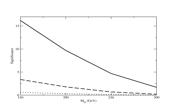
Figure 6: Significance of the two-Higgs signal in the Little Higgs model with respect to the Standard model, at the LHC, assuming an integrated luminosity of 10 $fb^{-1}$. Solid, dashed and dotted lines correspond to $f=$ $500$, $1000$ and $2000$ GeV, respectively.

V Conclusions

The double Higgs production process probes the nature of the electroweak symmetry breaking mechanism. This process is intimately tied to the cancellation of quadratic divergences in Little Higgs models. Here we have studied the reach of the LHC to probe the LH models in this way. We found that only for relatively small values of the energy scale $f$, of the order of $500$ to $1000$ GeV, it is possible to distinguish meaningfully the LH from the SM. These low values are attainable without violating the electroweak precision limits only in models where an extra T parity is incorporated TParity9 . On the other hand, these results only mildly dependent on the heavy top quark mass $m_{T}$; while the situation is more promising for larger values of $m_{T}$, it becomes practically independent of it for $m_{T}$ above $2.5$ TeV.

References

• (1) See e.g., S.P. Martin, A supersymmetry primer, in “Perspectives in Supersymmetry”, edited by G.L. Kane, World Scientific [hep-ph/9709356].
• (2) For a recent review, see C.T. Hill and E.H. Simmons, Strong dynamics and electroweak symmetry breaking, Phys. Rept. 381 (2003) 235, [hep-ph/0203079].
• (3) N. Arkani-Hamed, A.G. Cohen and H. Georgi, Electroweak symmetry breaking from dimensional deconstruction, Phys. Lett. B 513 (2001) 232 [hep-ph/0105239]; N. Arkani-Hamed, A.G. Cohen, T. Gregoire and J.G. Wacker, Phenomenology of electroweak symmetry breaking from theory space, JHEP 0208 (2002) 020, [hep-ph/0202089]; N. Arkani-Hamed, A.G. Cohen, E. Katz, A.E. Nelson, T. Gregoire and J.G. Wacker, The minimal moose for a little higgs, JHEP 0208 (2002) 021, [hep-ph/0206020].
• (4) C. Csaki, J. Hubisz, G.D. Kribs and P. Meade, Big corrections from a little higgs, Phys. Rev. D67 (2003) 115002, [hep-ph/0211124]; C. Csaki, J. Hubisz, G.D. Kribs and P. Meade, Variations of little higgs models and their electroweak constraints, Phys. Rev. D68 (2003) 035009, [hep-ph/0303236] ; J.L. Hewett, F.J. Petriello and T.G. Rizzo, Constraining the littlest higgs, JHEP 0310 (2003) 062 [hep-ph/0211218]; M.C. Chen and S. Dawson, One loop radiative corrections to the rho parameter in the littlest higgs model Phys. Rev. D70 (2004) 015003, [hep-ph/0311032].
• (5) G. Burdman, M. Perelstein and A. Pierce, Large hadron collider tests of a little higgs model, Phys. Rev. Lett. 90, (2003) 241802 and Erratum-ibid. 92, (2004) 049903, [hep-ph/0212228]; C. Dib, R. Rosenfeld and A. Zerwekh, Higgs production and decay in the little higgs models, [hep-ph/0302068] (unpublished); T. Han, H.E. Logan, B. McElrath and L.-T. Wang, Phenomenology of the little higgs model, Phys. Rev. D67 (2003) 095004, [hep-ph/0301040]; T. Han, H.E. Logan, B. McElrath and L.-T. Wang, Loop induced decays of the little higgs, Phys. Lett. B563 (2003) 191 and Erratum-ibid. B603 (2004) 257 (2004), [hep-ph/0302188]; T. Han, H.E. Logan, B. McElrath and L.-T. Wang, Smoking-gun signatures of little higgs models, [hep-ph/0506313].
• (6) For a recent review, see e. g., M. Schmaltz and D. Tucker-Smith, Little higgs review, [hep-ph/0502182].
• (7) N. Arkani-Hamed, A.G. Cohen, E. Katz, and A.E. Nelson, The littlest higgs, JHEP 0207 (2002) 034 .
• (8) M. Perelstein, M.E. Peskin and A. Pierce, Top quarks and electroweak symmetry breaking in little higgs models, Phys. Rev. D69 (2004) 075002, [hep-ph/0310039] .
• (9) We noticed that this condition was not satisfied for the values of the couplings and masses given in Han et al., ref. pheno5 .
• (10) H.C. Cheng and I. Low, TeV Symmetry and the Little Hierarchy Problem, JHEP bf 0309 (2003) 051, [hep-ph/0308199]; H.C.  Cheng and I. Low, Little Hierarchy, Little Higgses, and a Little Symmetry, JHEP bf 0408 (2004) 061, [hep-ph/0405243]; I. Low, T Parity and the Littlest Higgs, JHEP bf 0410 (2004) 067, [hep-ph/0409025]; J. Hubisz and P. Meade, it Phenomenology of the Littlest Higgs with T-Parity, Phys. Rev. D71 (2005) 035016, [hep-ph/0411264]; J. Hubisz, P. Meade, A. Noble and M. Perelstein, Electrowaek precision constraints on the littlest higgs model with T-parity, [hep-ph/0506042].
• (11) See e.g., T. Plehn, M. Spira and P.M. Zerwas, Pair production of neutral higgs particles in gluon-gluon collisions, Nucl. Phys. B479 (1996) 46 and Erratum ibid. 531 (1998) 655, [hep-ph/9603205]; A. Djouadi, W. Kilian, M. Muhlleitner and P. M. Zerwas, Production of neutral higgs boson pairs at LHC, Eur. Phys. J. C10 (1999) 45, [hep-ph/9904287].
• (12) G. Passarino and M. J. G. Veltman, One loop corrections for e+ e- annihilation into $\mu^{+}\mu^{-}$ in the Weinberg model, Nucl. Phys. B 160 (1979) 151 .
• (13) R. Mertig, M. Böhm and A. Denner, FeynCalc: computer algebraic calculation of Feynman amplitudes, Comput.  Phys.  Commun. 64 (1991) 345.
• (14) T. Hahn and M. Perez-Victoria, Automatized one-loop calculations in four dimensions and in D dimensions, Comput.  Phys.  Commun. 118 (1999) 153, [hep-ph/9807565].
• (15) J. Pumplin et al. (CTEQ Collaboration), New generation of parton distributions with uncertainties from global QCD analysis, JHEP 0207 (2002) 012, [hep-ph/0201195].
• (16) S. Dawson, S. Dittmaier and M. Spira, Neutral higgs-boson pair production at hadron colliders: QCD corrections, Phys. Rev. D 58 (1998) 115012, [hep-ph/9805244].
• (17) Liu Jing-Jing, Ma Wen-Gan, Li Gang, Zhang Ren-You and Hou Hong-Sheng, Higgs boson pair production in the little higgs model at hadron colliders, Phys. Rev. D 70 (2004) 015001, [hep-ph/0404171].
• (18) U. Baur, T. Plehn and D. Rainwater, Determining the Higgs boson self-coupling at hadron colliders, Phys. Rev. D 67 (2003) 033003, [hep-ph/0211224]; U. Baur, T. Plehn and D. Rainwater, Probing the Higgs self-coupling at hadron colliders using rare decays, Phys. Rev. D 69 (2004) 053004, [hep-ph/0310056].