IFJPAN-V-05-09
CERN-PH-TH/2005-146

Constrained non-Markovian Monte Carlo modelling of the evolution equation in QCD^⋆

S. Jadach and M. Skrzypek

Institute of Nuclear Physics, Academy of Sciences,
ul. Radzikowskiego 152, 31-342 Cracow, Poland,
and

CERN Department of Physics, Theory Division
CH-1211 Geneva 23, Switzerland

A new class of the constrained Monte Carlo (CMC) algorithms for the QCD evolution equation was recently discovered. The constraint is imposed on the type and the total longitudinal energy of the parton exiting QCD evolution and entering a hard process. The efficiency of the new CMCs is found to be reasonable.

Contribution to the HERA–LHC Workshop, 2004–2005

IFJPAN-V-05-09
CERN-PH-TH/2005-146

^⋆Supported in part by the EU grant MTKD-CT-2004-510126, in partnership with the CERN Physics Department.

1 Introduction

This brief report summarizes the recent developments in the area of the Monte Carlo (MC) techniques for the perturbative QCD calculations. Most of it was done at the time of the present HERA–LHC workshop, partial results being presented at several of its meetings. At present, two papers, [1] and [2], demonstrating the principal results are already available. Generally, these MC techniques concern the QCD evolution of the parton distribution functions (PDFs) $D_{k}(x,Q)$, where $k$ denotes the type of the parton (quark, gluon), $x$ the fraction of longitudinal momentum of the initial hadron carried by the parton, and the size of the available real/virtual emission phase space is $Q$. The evolution equation describes the response of the PDF to an increase of $Q$; $D_{k}(x,Q)$ is an inclusive distribution and can be measured almost directly in hadron–lepton scattering. On the other hand, it was always known that there exists in QCD an exclusive picture of the PDF, the so-called parton-shower process, in which $D_{k}(x,Q)$ is the distribution of the parton exiting the emission chain and entering the hard process (lepton–quark for example). The kernel functions $P_{kj}(Q,z)$, that govern the differential evolution equations of PDFs are closely related to distributions governing a single emission process $(i-1)\to i$ in the parton shower: $P_{k_{i}k_{i-1}}(Q_{i},x_{i}/x_{i-1})$.

In other words, the evolution ($Q$-dependence) of PDFs and the parton shower represent two faces of the same QCD reality. The first one (inclusive) is well suited for basic precision tests of QCD at hadron–lepton colliders, while the second one (exclusive) provides realistic exclusive Monte Carlo modelling, vitally needed for experiments at high-energy particle colliders.

At this point, it is worth stressing that, so far, we were referring to DGLAP-type PDFs [3] and their evolution, and to constructing a parton-shower MC starting from them, as was done two decades ago and is still done today. This involves a certain amount of “backward engineering” and educated guesses, because the classical inclusive PDFs integrate over the $p_{T}$ of the exiting parton. The so-called unintegrated PDFs (UPDFs) $D_{k}(x,p_{T},Q)$ would be more suitable for the purpose, leading to higher-quality QCD calculations. UPDFs are, however, more complicated to handle, both numerically and theoretically. (It is still a challenge to construct a parton-shower MC based consistently on the theoretically well defined UPDFs.)

Another interesting “entanglement” of the evolution of PDFs on one side and of the parton shower (PS) MC on the other side is also present in the modelling of the showering of the incoming hadron – mostly for technical reasons and convenience. The Markovian nature of the QCD evolution can be exploited directly in the PS MC, where partons split/decay as long as there is enough energy to dissipate (final state) or the upper boundary $Q$ of the phase space is hit (initial state). The multiparton distribution in such a MC is a product of the evolution kernels. However, such a direct Markovian MC simulation of a shower is hopelessly inefficient in the initial state, because the hard process accepts only certain types and momenta of the incoming partons – most of the shower histories are rejected (zero MC weight) by the hard process. This is especially true for forming narrow resonances such as electroweak bosons or Higgs boson at the LHC. The well known “workaround” is the backward evolution MC algorithm of Sjöstrand, used currently in all PS MCs, such as HERWIG [4] and PYTHIA [5]. Contrary to the forward Markovian MC, where the physics inputs are PDFs at low $Q_{0}\sim$1 GeV and the evolution kernels, in the backward evolution MC one has to know PDFs in the entire range $(Q_{0},Q)$ from a separate non-MC numerical program solving the evolution equation and setting up look-up tables (or numerical parametrization) for them.

The following question has been pending in the parton-shower MC methodology for a long time: Could one invent an efficient “monolithic” MC algorithm for the parton shower from the incoming hadron, in which no external PDFs are needed and the only input are PDFs at $Q_{0}$ and the evolution kernel (the QCD evolution being a built-in feature of the parton shower MC)? Another question rises immediately: Why bother? Especially since this is a tough technical problem. This cannot still be fully answered before the above technique is applied in the full-scale (four-momentum level) PS MC. Generally, we hope that this technique will open new avenues in the development of the PS MC at the next-to-leading-logarithmic (NLL) level. In particular, it may help in constructing PS MCs closely related to unintegrated structure functions and, secondly, it may provide a better integration of the NLL parton shower (yet to be implemented!) with the NLL calculation for the hard process.

The first solution of the above problem of finding an efficient “constrained MC” (CMC) algorithm for the QCD evolution was presented in refs. [1, 6]. This solution belongs to what we call a CMC class II, and it relies on the observation that all initial PDFs at $Q_{0}$ can be approximated by $\hbox{const}\cdot x_{0}^{\eta-1}$; this is to be corrected by the MC weight at a later stage. This allows elimination of the constraint $x=\prod_{i}z_{i}$, at the expense of $x_{0}$, keeping the factorized form of the products of the kernels. Simplifying phase-space boundaries in the space of $z_{i}$ is the next ingredient of the algorithm. Finally, in order to reach a reasonable MC efficiency for the pure bremsstrahlung case out of the gluon emission line, one has to generate a $1/z$ singularity in the $G\to G$ kernel in a separate branch of the MC. The overall efficiency of the MC is satisfactory, as is demonstrated in ref. [1] for the case of the pure bremsstrahlung out of the gluon and quark colour charge. Generalization to the quark–gluon transition is outlined, but not yet implemented. The main drawback of this method is its algebraic complexity. Further improvement of its relatively low MC efficiency is possible (even though it could lead to even more algebraic complexity).

The second, more efficient, CMC algorithm was presented in ref. [2] (as well as during the October 2004 meeting of the workshop). It belongs to what we call a CMC class I. The main idea is to project/map points from the hyperspace defined by the energy constraint $x=\prod_{i}z_{i}$, into a simpler hyperspace, defined by the hardest emission, $x=\min z_{i}$. This mapping is accompanied by the appropriate MC weight, which compensates exactly for the deformation of the distributions involved, and the bookkeeping of the hyperspace boundaries is rigorous. The above describes a CMC for the pure bremsstrahlung segment of the gluon emission out of a quark or gluon chain. Many such segments are interconnected by the quark–gluon transitions. The algebraic hierarchic reorganization of the emission chain into a super-level of the quark–gluon transitions and sub-level of the pure bremsstrahlung is an important ingredient in all CMC algorithms and will be published separately [7]. The basic observation made in ref. [8] is that the average number of super-level transitions is low, $\sim 1$; hence for precision of a $10^{-4}$ it is sufficient to limit it to three or four transitions. The integration/simulation of the super-level variables is done efficiently using the general-purpose MC tool FOAM [9, 10]. The above proof of the correctness of the CMC class I algorithm concept was given in ref. [2] for the full DGLAP-type QCD evolution with the LL kernels (including quark–gluon transitions).

Although our main aim is to construct the non-Markovian CMC class of algorithms, we have developed in parallel the family of Markovian MC (MMC) algorithms/programs, which provide numerical solutions of the QCD evolution equations with high precision, $\sim 10^{-3}$. We use them at each step of the CMC development as numerical benchmarks for the precision tests of the algorithms and their software implementations. The first example of MMC for DGLAP at LL was defined/examined in ref. [8] and tested using the non-MC program QCDnum16 [11]. In some cases our MMC programs stand ahead of their CMC brothers; for instance, they already include NLL DGLAP kernels. A systematic description of the MMC family of our MC toolbox is still under preparation [13].

The last development at the time of the workshop was an extension of the CMC type-I algorithm from DGLAP to CCFM one-loop evolution [14] (also referred to as HERWIG evolution [15]), in which the strong coupling constant gains $z$-dependence, $\alpha_{s}(Q)\to\alpha_{s}(Q(1-z))$, as advocated in ref. [16], confirmed by NLL calculations [17]. The above ansatz also compels introduction of a $Q$-dependent IR cutoff, $\varepsilon=Q_{\varepsilon}/Q$: another departure from DGLAP. This version of the CMC is still unpublished. Its version for the pure bremsstrahlung was presented at the March 2005 meeting of the workshop; in particular a perfect numerical agreement with the couterpartner MMC was demonstrated. Recently both CMC and MMC for the one-loop CCFM were extended to quark–gluon transitions, and again perfect agreement was found.

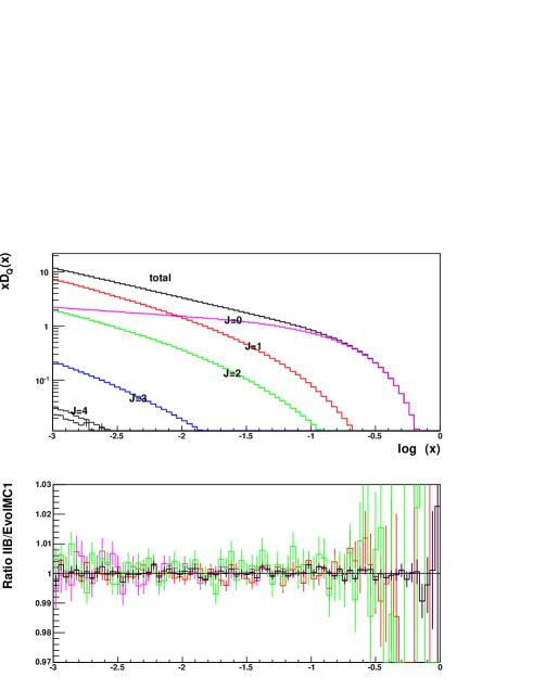
Figure 1: CMC of the one-loop CCFM versus the corresponding MMC for quarks; number of quark–gluon transitions $J=0,1,2,3,4$, and the total. The ratios in the lower plot are for $n=0,1$ and the total (blue).

For the detailed description of the new CMC algorithm, we refer the reader to the corresponding papers [1] and [2] and workshop presentations. Here, let us only show one essential step in the development of the CMC for the one-loop CCFM model – the mapping of the Sudakov variables for the pure bremsstrahlung:

$$\begin{split}I&=\int_{t_{0}}^{t_{1}}dt\int_{0}^{z_{1}}dz\;\alpha(Q(1-z))\;zP^{\Theta}_{GG}(z,t)\\ &=\frac{2}{\beta_{0}}\int_{0}^{z_{1}}dz\int_{t_{0}}^{t_{1}}dt\;\frac{1}{{\hat{t}}+\ln(1-z)}\frac{\theta_{\ln(1-z)>{\hat{t}}_{\varepsilon}-{\hat{t}}}}{1-z}=\frac{2}{\beta_{0}}\int_{0}^{y_{\max}}dy(z)\int_{0}^{1}ds(t).\end{split}$$ (1)

The short-hand notation ${\hat{t}}={\hat{t}}(t)\equiv t-t_{\Lambda}$ and $v=\ln(1-z)$ supplements that of ref. [2] in use, and the mapping reads

$$\begin{split}&y(z)=\rho(v_{1};{\hat{t}}_{1},{\hat{t}}_{0})=\rho(v_{1}+{\hat{t}}_{1})-\theta_{v_{1}>t_{\varepsilon}-t_{0}}\rho(v_{1}+{\hat{t}}_{0}),\quad s(t)=\frac{\ln({\hat{t}}+v)}{\rho^{\prime}(v;{\hat{t}}_{1},{\hat{t}}_{0})},\qquad\\ &\rho^{\prime}(v;{\hat{t}}_{1},{\hat{t}}_{0})=\theta_{v<t_{\varepsilon}-t_{0}}\rho^{\prime}(v+{\hat{t}}_{1})+\theta_{v>t_{\varepsilon}-t_{0}}[\rho^{\prime}(v+{\hat{t}}_{1})-\rho^{\prime}(v+{\hat{t}}_{0})],\end{split}$$ (2)

where $\rho(t)\equiv{\hat{t}}(\ln{\hat{t}}-\ln{\hat{t}}_{\varepsilon})+{\hat{t}}_{\varepsilon}-{\hat{t}}$. Once the above mapping is set, the same algorithm, with the parallel shift $y_{i}\to y_{i}+Y$, can be used in this case. The super-level of quark–gluon transitions is again implemented using FOAM. A numerical comparison of the corresponding CMC and MMC programs is shown in fig. 1. The MC efficiency is comparable with that of the DGLAP case.

Summary: We have constructed and tested new, efficient, constrained MC algorithms for the initial-state parton-emission process in QCD.

References

- [1] S. Jadach and M. Skrzypek, report IFJPAN-V-04-06, hep-ph/0504205, Acta Phys. Pol. in press.
- [2] S. Jadach and M. Skrzypek, report IFJPAN-V-04-07, hep-ph/0504263.
-
[3]
L.N. Lipatov, Sov. J. Nucl. Phys. 20 (1975) 95;
V.N. Gribov and L.N. Lipatov, Sov. J. Nucl. Phys. 15 (1972) 438;
G. Altarelli and G. Parisi, Nucl. Phys. 126 (1977) 298;
Yu. L. Dokshitzer, Sov. Phys. JETP 46 (1977) 64. - [4] G. Corcella et al., JHEP 01 (2001) 010, hep-ph/0011363.
- [5] T. Sjöstrand et al., Comput. Phys. Commun. 135 (2001) 238–259, hep-ph/0010017.
- [6] S. Jadach and M. Skrzypek, Nucl. Phys. Proc. Suppl. 135 (2004) 338–341.
- [7] S. Jadach, M. Skrzypek, and Z.Wa̧s, Report IFJPAN-V-04-09.
- [8] S. Jadach and M. Skrzypek, Acta Phys. Polon. B35 (2004) 745–756, hep-ph/0312355.
- [9] S. Jadach, Comput. Phys. Commun. 152 (2003) 55–100, physics/0203033.
- [10] S. Jadach and P. Sawicki, physics/0506084.
- [11] M. Botje, ZEUS Note 97-066, http://www.nikhef.nl/ h24/qcdcode/.
- [12] K. Golec-Biernat, APCheb33, the Fortran code to be obtained from the author; unpublished.
- [13] K. Golec-Biernat, S. Jadach, M. Skrzypek, and W. Płaczek, report IFJPAN-V-05-03.
-
[14]
M. Ciafaloni, Nucl. Phys. B296 (1988) 49;
S. Catani, F. Fiorani, and G. Marchesini, Phys. Lett. B234 339, Nucl. Phys. B336 (1990) 18. - [15] P. Nason, JHEP 11 (2004) 040, hep-ph/0409146.
- [16] D. Amati, A. Bassetto, M. Ciafaloni, G. Marchesini, and G. Veneziano, Nucl. Phys. B173 (1980) 429.
- [17] G. Curci, W. Furmanski, and R. Petronzio, Nucl. Phys. B175 (1980) 27.