MADPH-05-1441 SLAC-PUB-11472

2005 ALCPG & ILC Workshops - Snowmass, U.S.A.
Probing the Universal Randall-Sundrum Model at the ILC

Abstract

The Randall-Sundrum model with all Standard Model (SM) fields in the bulk, including the Higgs, can be probed by precision measurements at the ILC. In particular, the couplings of the Higgs to the gauge bosons of the SM can be determined with high accuracy at the ILC. Here we examine the deviations in these couplings from their SM values within the framework of the Universal Randall-Sundrum Model (URSM) as well as the corresponding couplings of the first Higgs Kaluza-Klein excitation.

The Randall-Sundrum (RS) model provides an interesting explanation of the hierarchy problemRandall:1999ee . In the original RS model, the only 5-d field is the graviton. Since that time numerous works have extended the RS setup to include bulk fermions and gauge fieldsDavoudiasl:2005uu . However, even though the SM can be promoted to a 5-d theory, the fundamental Higgs field responsible for electroweak symmetry breaking (EWSB) has been kept on the TeV-brane. The reason for this has been to avoid problems associated with extreme fine-tuning and conflict with known experimental data. There have also been attempts to build RS models without fundamental Higgs bosons where the role of the Higgs doublet as a source of Goldstone bosons is played by the fifth components of the gauge fields themselves.

We have recently shownDavoudiasl:2005uu that by appropriate choices of the Higgs sector parameters in the bulk and on both the TeV and Planck branes, one can generate a single tachyonic Kaluza-Klein (KK) mode of the Higgs field in the low energy 4-d theory. This tachyonic mode can be identified as the SM Higgs field. Given a quartic bulk term for the Higgs, the tachyonic mode will lead to the usual 4-d Higgs mechanism and endow the electroweak gauge bosons with mass. A particularly interesting realization of this “Off-the-Wall” Higgs EWSB employs the gravitational sector of the RS model to provide the necessary bulk and brane mass scales. These scales are then related to the 5-d curvature of the RS geometry. Consequently, new relations and constraints among the parameters of the Higgs and gravitational sectors are obtained. In this gravity-induced EWSB scenario, the higher curvature Gauss-Bonnet terms play an important role. Typical generic signatures of our scenario are the emergence of a tower of Higgs KK modes as well as a modification of the $WWH$ coupling which can be directly probed through precision measurements at the ILC.

In order to understand the basic model let us focus on the free Higgs case (i.e., ignoring gauge and self-couplings as well as other particles such as the Goldstone bosons) which involves only the various mass terms. Studying this truncated action for the free Higgs field allows us to perform the KK decomposition $\phi\rightarrow\sum_{n}\phi_{n}(x)\chi_{n}(y)=\phi_{T}\chi_{T}+...$ where $\chi_{T}$ is the wavefunction for the tachyon and represents the shape of the Higgs vev profile in the bulk. We have

$$S_{trunc}=\int d^{5}x~{}\sqrt{-g}\Bigg{[}(\partial^{A}\phi)^{\dagger}(\partial_{A}\phi)-m^{2}\phi^{\dagger}\phi+{1\over{k}}\phi^{\dagger}\phi~{}[\mu_{P}^{2}\delta(y)-\mu_{H}^{2}\delta(y-\pi r_{c})]\Bigg{]}\,.$$ (1)

To scale out dimensional factors we define $m^{2}=20k^{2}\xi$ and $\mu_{P,H}^{2}=16k^{2}\xi\beta_{P,H}$ since $k$ is the canonical scale for RS masses. Recall that the RS metric is given by $ds^{2}=e^{-2k|y|}\eta_{\mu\nu}dx^{\mu}dx^{\nu}-dy^{2}$ where we use $-\pi r_{c}\leq y\leq\pi r_{c}$ as the 5-d coordinate and $k$ is the curvature parameter whose value is comparable to that of the fundamental scale $M$. Note that the parameters $\xi,\beta_{P,H}$ are dimensionless and are expected to be $O(1)$ but may, in principle, be of arbitrary sign. What we looking for in the $(\xi,\beta_{P,H})$ parameter space is to obtain EWSB in a manner consistent with the SM; our basic criterion is to find regions where there exists one, and only one, TeV scale tachyonic mode that we can identify with the SM Higgs. The remaining Higgs KK tower fields must also be normal, i.e., non-tachyonic. To this end we solve the equation of motion for the Higgs KK wavefunctions:

$$\partial_{y}\Big{(}e^{-4k|y|}\partial_{y}\chi_{n}\Big{)}-m^{2}e^{-4k|y|}\chi_{n}+{1\over{k}}e^{-4\sigma}[\mu_{P}^{2}\delta(y)-\mu_{H}^{2}\delta(y-\pi r_{c})]\chi_{n}+m_{n}^{2}e^{-2k|y|}\chi_{n}=0\,,$$ (2)

and apply the appropriate boundary conditions on both the TeV and Planck branesDavoudiasl:2005uu ; one can show that $\beta_{P}$ plays no essential role in the solutions of interest to us. We find that if the combination $\xi\beta_{H}>0$ then either no tachyon exists or that the resulting Higgs vev is Planck scale. Clearly, we must instead choose the parameters such that $\xi\beta_{H}<0$. In this case their are two remaining regions: (I)$\xi>0,~{}\beta_{H}<0$ or (II)$\xi<0,~{}\beta_{H}>0$. Furthermore, we find that within both of these regions further constraints on the parameters must apply in order that a tachyon root exist: $\xi\geq(\leq)\xi_{1,2}$ in region I(II). $\xi_{1,2}$ are given by the expressions $\xi_{1}=-{1\over{4\beta_{H}}}$ and $\xi_{2}={{5-8\beta_{H}}\over{16\beta_{H}^{2}}}$. We note that region II is favored by the “gravity-induced” EWSB mechanism since in that region it is easy to avoid ghosts in the radion and graviton sectors. Clearly the detailed nature of the solutions for the bulk Higgs profile $\chi_{T}$ will depend on the particular values of the parameters $\xi,~{}\beta_{H}$. One finds that the Higgs profile is highly peaked near the TeV brane, $\chi_{T}\sim e^{(2+\nu)k|y|}$ where $\nu^{2}=4+20\xi$. The masses of the Higgs boson and its KK excitations are found to be given by the roots, $x_{n}$, of a transcendental equation involving Bessel functions of order $\nu$ and depend on the values of both $\xi$ and $\beta_{H}$.

Let us now turn to the gauge boson couplings of the Higgs in URSM. In the SM the $W$ boson gets its mass directly from the vev of the Higgs boson. In the case of the URSM, the $W$ has an additional, geometric, mass source arising solely from back reaction, i.e., wavefunction curvature. This implies that the $HWW$ (and, hence, $HZZ$) coupling will be somewhat smaller than that obtained in the SM. The relevant coupling can be expressed as an integral over $y$:

$$S_{eff}=\int d^{4}x~{}HW_{\mu}^{\dagger}W^{\mu}~{}{1\over{4\pi r_{c}}}g^{2}v\int~{}dy~{}e^{-2k|y|}\chi_{T}^{2}f_{0}^{2}\,,$$ (3)

where $v$ is the Higgs vev, $g$ is the usual 4-d coupling assuming that the light SM fermions are localized near the Planck brane, and $f_{0}(y)$ is the $W=W_{0}$ boson KK wavefunction. (It is important to note at this point that $v$ need not be $v_{SM}\simeq 246$ GeV.) These are obtained by KK expanding the 5-d $W$ field $W=\sum_{n}W_{n}(x)f_{n}(y)$ and solving the mode equation

$$\partial_{y}\Big{(}e^{-2k|y|}\partial_{y}f_{n}\Big{)}-{1\over{4}}g_{5}^{2}v^{2}\chi_{T}^{2}e^{-2k|y|}f_{n}+m_{n}^{2}f_{n}=0\,,$$ (4)

where $g=g_{5}/{\sqrt{2\pi r_{c}}}$ is the 5-d $SU(2)_{L}$ gauge coupling, with suitable boundary conditions. In this language the $W$ boson mass is given by

$$M_{W}^{2}={1\over{4}}2\pi r_{c}g^{2}v^{2}\int~{}dy~{}e^{-2k|y|}f_{0}^{2}\chi_{T}^{2}+\int~{}dy~{}e^{-2k|y|}(\partial_{y}f_{0})^{2}\,.$$ (5)

     

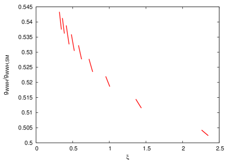
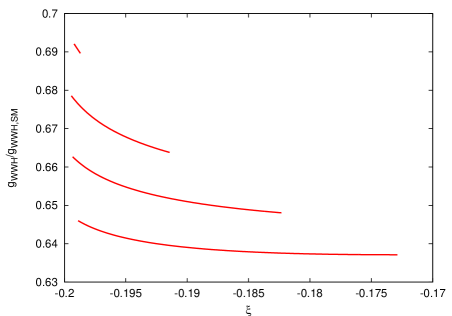
Figure 1: Values of the coupling ratio $g_{WWH}/g^{SM}_{WWH}$ in regions I (left) and II (right) as functions of $\xi$ for various $\beta_{H}$. In region I, from top from top to bottom, the curves correspond to $\beta_{H}=1.4,1.6,1.8,2.0$. A cut on the Higgs boson mass as described in the text has been imposed.

How do the $WWH$ couplings in the URSM compare to their SM values, i.e., what are ratios $g_{WWH}/g^{SM}_{WWH}$ as we scan over the $\xi-\beta_{H}$ parameters in the two regions? The results of such a scan are shown in Fig. 1 for both regions I and II in units of $v/v_{SM}$ which we expect to be O(1); these results have been subjected to the additional requirement that the tachyon root, $x_{T}$, satisfy the bound $x_{T}<2$ so that the resulting Higgs mass lies below a TeV and, hence, is visible at LHC/ILC. Here we see that results in the two regions are quite different with much larger deviations from the SM seen in region I. It is important to note that not only are these deviations significant but they are restricted to a rather unique, narrow ranges in either region. With precision measurements at the ILC these predictions can be directly tested. The ratio $v/v_{SM}$ itself can be independently determined by combining the Higgs mass measurement with that of the 4-d quartic coupling via the relation $\lambda_{4d}=m_{H}^{2}/(2v^{2})$. The first KK Higgs excitation may be light enough to be produced at a 1 TeV ILC so that it is important to examine these couplings as well which can be obtained in a manner similar to the above. The corresponding results can be seen in Fig. 2 for both regions where we see the previous pattern repeated. The reduced values of these couplings will lead to a substantial reduction in the production cross section for this state making it difficult to produce at LHC/ILC.

     

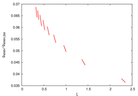
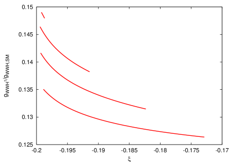
Figure 2: Same as the previous figure but now for the first Higgs KK excitation.

In the “gravity-induced” version of the URSM there are additional predictions which may be testable at the ILC. In this framework the parameter $\xi$ controls the size of Higgs-radion mixing which is now directly correlated with the $HWW$ coupling in the weak eigenstate basis. Measurements of radion properties will provide further tests of the URSM scenario.

- (1) L. Randall and R. Sundrum, Phys. Rev. Lett. 83, 3370 (1999) [arXiv:hep-ph/9905221].
- (2) For details of the present work and original references, see H. Davoudiasl, B. Lillie and T. G. Rizzo, arXiv:hep-ph/0508279.