DESY 05-207

LAL 05-98

hep-ph/0509159

September 15, 2005

Physics at Future Linear Colliders
K. Mönig
DESY, Zeuthen, Germany and LAL, Orsay France
E-mail: klaus.moenig@desy.de

This article summarises the physics at future linear colliders. It will be shown that in all studied physics scenarios a 1 TeV linear collider in addition to the LHC will enhance our knowledge significantly and helps to reconstruct the model of new physics nature has chosen.

Invited talk at the Lepton Photon Symposium 2005, Upsala, Sweden, July 2005

1 Introduction

Most physicists agree that the International Linear Collider, ILC, should be the next large scale project in high energy physics[1]. The ILC is an $\mathrm{e}^{+}\mathrm{e}^{-}$ linear collider with a centre of mass energy of $\sqrt{s}\leq 500{\,\mathrm{Ge\kern-1.00006ptV}}$ in the first phase, upgradable to about $1{\,\mathrm{Te\kern-1.00006ptV}}$[2]. The luminosity will be ${\cal L}\approx 2-5\cdot 10^{34}\mathrm{cm}^{-2}\mathrm{s}^{-1}$ corresponding to $200-500\,\,{\rm fb}^{-1}$/year. The electron beam will be polarisable with a polarisation of ${\cal P}=80-90\%$.

In addition to this baseline mode there are a couple of options whose realisation depends on the physics needs. With relatively little effort also the positron beam can be polarised with a polarisation of $40-60\%$. The machine can be run on the Z resonance producing $>10^{9}$ hadronically decaying Z bosons in less than a year or at the W-pair production threshold to measure the W-mass to a precision around $6{\,\mathrm{Me\kern-1.00006ptV}}$ (GigaZ). The ILC can also be operated as an ${\rm e}^{-}{\rm e}^{-}$ collider. With much more effort one or both beams can be brought into collision with a high power laser a few mm in front of the interaction point realising a $\gamma\gamma$ or ${\rm e}\gamma$ collider with a photon energy of up to 80% of the beam energy.

At a later stage one may need an $\mathrm{e}^{+}\mathrm{e}^{-}$ collider with $\sqrt{s}=3-5{\,\mathrm{Te\kern-1.00006ptV}}$. Such a collider may be realised in a two-beam acceleration scheme (CLIC). Extensive R&D for such a machine is currently going on[3].

ILC will run after LHC[4, 5] has taken already several years of data. However the two machines are to a large extend complementary. The LHC reaches a centre of mass energy of $\sqrt{s}=14{\,\mathrm{Te\kern-1.00006ptV}}$ leading to a very high discovery range. However not the full $\sqrt{s}$ is available due to parton distributions inside the proton ($\sqrt{s}_{\rm eff}\sim 3{\,\mathrm{Te\kern-1.00006ptV}}$). The initial state is unknown and the proton remnants disappear in the beampipe so that energy-momentum conservation cannot be employed in the analyses. There is a huge QCD background and thus not all processes are visible.

ILC has with its $\sqrt{s}\leq 1{\,\mathrm{Te\kern-1.00006ptV}}$ a lower reach for direct discoveries. However the full $\sqrt{s}$ is available for the primary interaction and the initial state is well defined, including its helicity. The full final state is visible in the detector so that energy-momentum conservation also allows reconstruction of invisible particles. Since the background is small, basically all processes are visible at the ILC.

The LHC is mainly the “discovery machine” that can find new particles up to the highest available energy and should show the direction nature has taken. On the contrary ILC is the “precision machine” that can reconstruct the underlying laws of nature. Only a combination of the LHC reach with the ILC precision is thus able to solve our present questions in particle physics.

Better measurement precision can not only improve existing knowledge but allows to reconstruct completely new effects. For example Cobe discovered the inhomogeneities of the cosmic microwave background but only the precision of WMAP allowed to conclude that the universe is flat. As another example, from the electroweak precision measurements before LEP and SLD one could verify that the lepton couplings to the Z were consistent with the Standard Model prediction but only the high precision of LEP and SLD could predict the Higgs mass within this model.

The ILC has a chance to answer several of the most important questions in particle physics. Roughly ordered in the chances of the ILC to find some answers they are:

• How is the electroweak symmetry broken? The ILC can either perform a precision study of the Higgs system or see first signs of strong electroweak symmetry breaking.

• What is the matter from which our universe is made off? ILC has a high chance to see supersymmetric dark matter, also some other solutions like Kaluza Klein dark matter might give visible signals.

• Is there a common origin of forces? Inside supersymmetric theories the unification of couplings as well as of the SUSY breaking parameters can be checked with high precision.

• Why is there a surplus of matter in the universe? Some SUSY models of baryogenesis make testable predictions for the ILC. Also CP violation in the Higgs system should be visible.

• How can gravity be quantised? The ILC is sensitive to extra dimensions up scales of a few TeV and tests of unification in SUSY may give a hint towards quantum gravity at the GUT scale.

2 The Top Quark Mass and why we need it

ILC can measure the top mass precisely from a scan of the ${\mathrm{t}\bar{\mathrm{t}}}$ threshold. With the appropriate mass definition the cross section near threshold is well under control[6] (see fig. 1). With a ten-point scan an experimental precision of $\Delta m_{\mathrm{t}}=34{\,\mathrm{Me\kern-1.00006ptV}}$ and $\Delta\Gamma_{\rm t}=42{\,\mathrm{Me\kern-1.00006ptV}}$ is possible[7], so that, including theoretical uncertainties $\Delta m_{\mathrm{t}}(\overline{{\rm MS}})\approx 100{\,\mathrm{Me\kern-1.00006ptV}}$ can be reached.

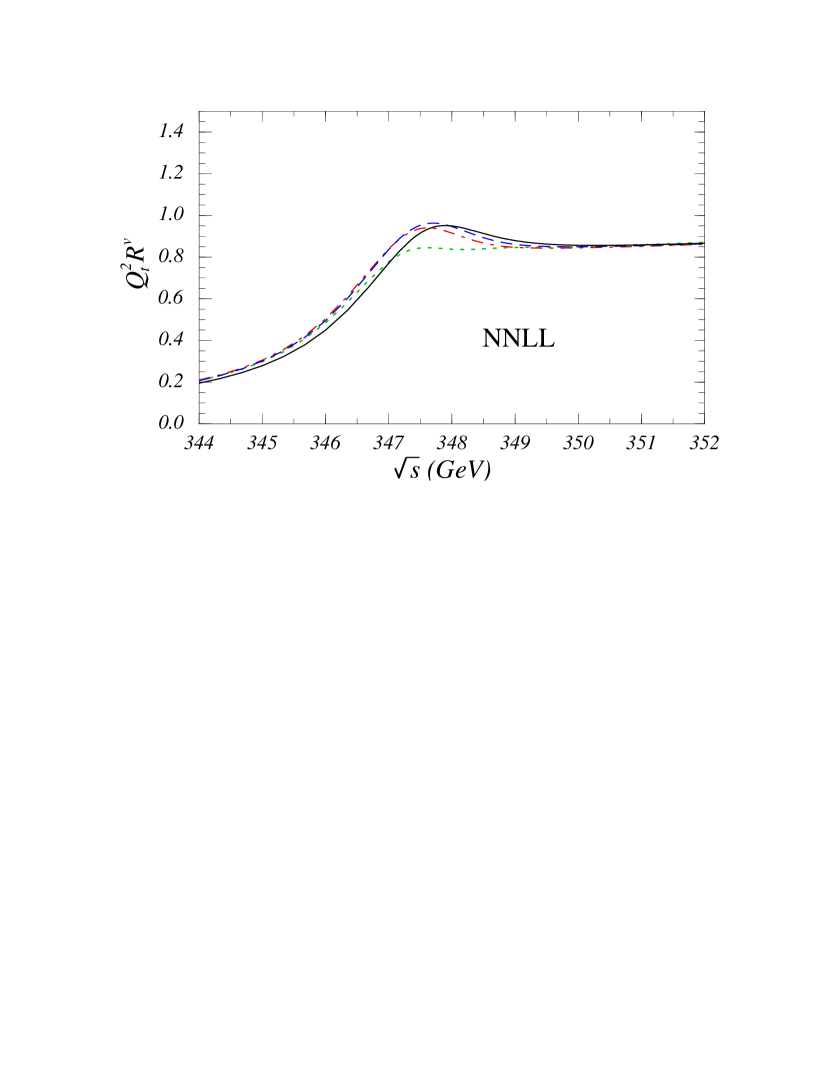
Figure 1: Top pair cross section using the NNLL pole mass for different values of the top velocity parameter[6].

A precise top mass measurement is needed in many applications. The interpretation of the electroweak precision data after GigaZ needs a top mass precision better than 2 GeV (fig. 2 left) and the interpretation of the MSSM Higgs system even needs a top mass precision of about the same size as the uncertainty on the Higgs mass (fig. 2 right)[8]. Also the interpretation of the WMAP cosmic microwave data in terms so the MSSM needs a good top mass precision in some regions of the parameter space[9].

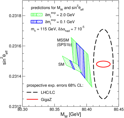
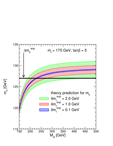
Figure 2: Required top mass precision for the interpretation of the electroweak precision data (left) and for the MSSM Higgs system (right).

3 Higgs Physics and Electroweak Symmetry Breaking

If a roughly Standard Model like Higgs exists, it will be found by the LHC. However the ILC has still a lot to do to figure out the exact model and to measure its parameters. If only one Higgs exists it can be the Standard Model, a little Higgs model or the Higgs can be mixed with a Radion from extra dimensions. If two Higgs doublets exist it can be a general two Higgs doublet model or the MSSM. However the Higgs structure may be even more complicated like in the NMSSM with an additional Higgs singlet or the top quark can play a special role as in little Higgs or top-colour models. In all cases there maybe only one Higgs visible at LHC that looks Standard-Model like, but the precision at ILC can distinguish between the models.

The Higgs can be identified independent from its decay mode using the $\mu^{+}\mu^{-}$ recoil mass in the process $\mathrm{e}^{+}\mathrm{e}^{-}\rightarrow HZ$ with $Z\rightarrow\mu^{+}\mu^{-}$ (see fig. 3)[10]. The cross section of this process is a direct measurement of the HZZ coupling and it gives a bias free normalisation for the Higgs branching ratio measurements. Together with the coss section of the WW fusion channel ($\mathrm{e}^{+}\mathrm{e}^{-}\rightarrow\nu\nu H$) this allows for a model independent determination of the Higgs width and its couplings to W, Z, b-quarks, $\tau$-leptons, c-quarks and gluons on the $1-5\%$ level[11].

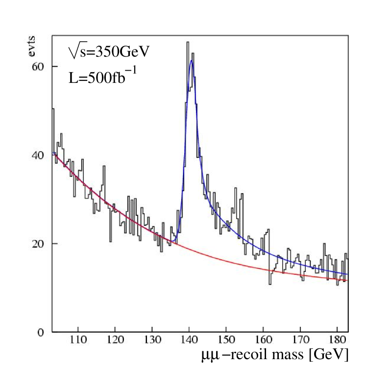
Figure 3: Measurement of $\mathrm{e}^{+}\mathrm{e}^{-}\rightarrow HZ$ from the $\mu^{+}\mu^{-}$ recoil mass.

At higher energies the ${\mathrm{t}\bar{\mathrm{t}}}H$ Yukawa coupling can be measured from the process $\mathrm{e}^{+}\mathrm{e}^{-}\rightarrow{\mathrm{t}\bar{\mathrm{t}}}H$ where the Higgs is radiated off a t-quark. At low Higgs masses, using $H\rightarrow{\mathrm{b}\bar{\mathrm{b}}}$, a precision around 5% can be reached. For higher Higgs masses, using $H\rightarrow WW$, 10% accuracy will be possible (see fig. 4)[12].

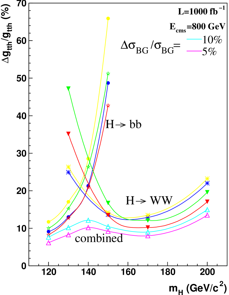
Figure 4: Expected precision of the ${\mathrm{t}\bar{\mathrm{t}}}H$ Yukawa coupling as a function of the Higgs mass.

If the Higgs is not too heavy the triple Higgs self-coupling can be measured to around 10% using the double-Higgs production channels $\mathrm{e}^{+}\mathrm{e}^{-}\rightarrow{\rm ZHH}$ and $\mathrm{e}^{+}\mathrm{e}^{-}\rightarrow\nu\bar{\nu}{\rm HH}$[13]. As shown in fig. 5 all these Higgs coupling measurements allow to show, that the Higgs really couples to the mass of the particles[13].

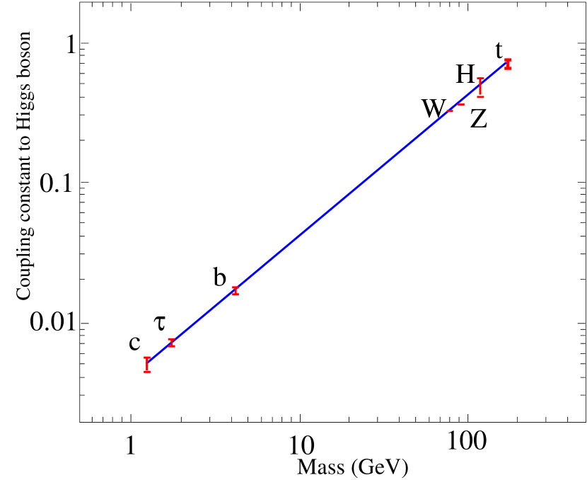
Figure 5: Higgs-particle coupling and expected uncertainty as a function of the particle mass.

These measurements present a powerful tool to test the model from which the Standard Model Higgs arises. Figure 6[13] shows possible deviations of the Higgs couplings from the the Standard Model prediction together with the expected uncertainties for a two Higgs doublet model, a model with Higgs-Radion mixing and a model incorporating baryogenesis[14]. In all cases the ILC allows to separate clearly between the Standard Model and the considered one.

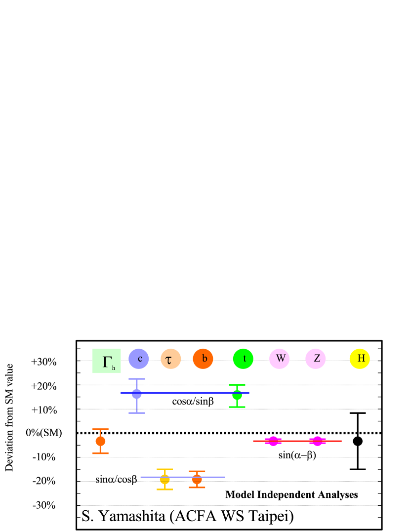
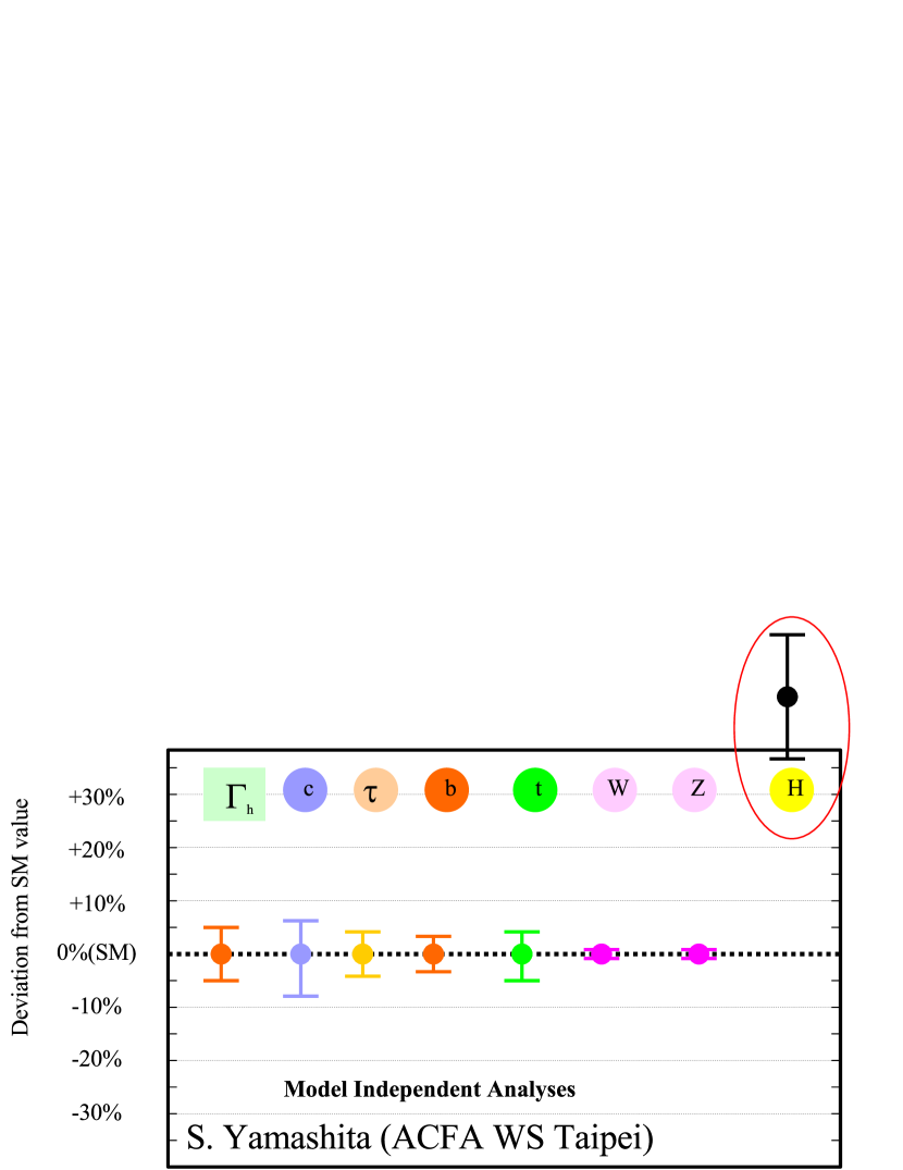
Figure 6: Deviation of the Higgs couplings from the Standard Model together with the expected ILC precision for a two Higgs doublet model (upper), a model with Higgs-Radion mixing (middle) and a model incorporating baryogenesis[14] (lower).

Further information can be obtained from loop decays of the Higgs, namely $H\rightarrow gg$ and $H\rightarrow\gamma\gamma$. Loop decays probe the Higgs coupling to all particles, also to those that are too heavy to be produced directly. The Higgs-decay into gluons probes the coupling to all coloured particles which is completely dominated by the top-quark in the Standard Model. The one to photons is sensitive to all charged particles, dominantly the top quark and the W-boson in the SM. The partial width $\Gamma(H\rightarrow gg)$ can be measured on the 5% level from Higgs decays in $\mathrm{e}^{+}\mathrm{e}^{-}$. The photonic coupling of the Higgs can be obtained from the Higgs production cross section at a photon collider (see fig. 7)[15, 16]. The loop decays of the Higgs are sensitive to the model-parameters in many models. As an example figure 8 shows the expected range of couplings within a little Higgs model[17].

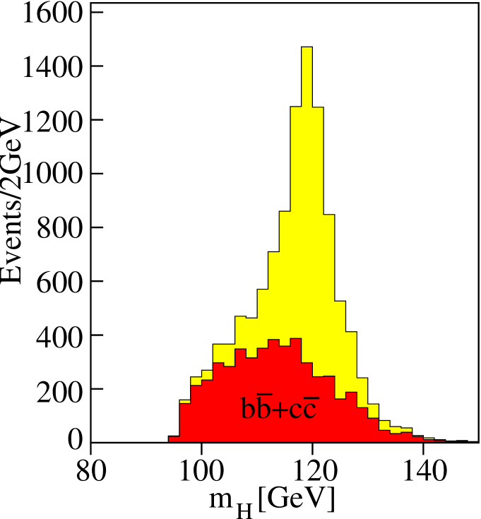
Figure 7: ${\mathrm{b}\bar{\mathrm{b}}}$ mass spectrum in the $\gamma\gamma\rightarrow H$ analysis after all cuts[15].

Figure 8: Possible deviations of Higgs loop decays from the Standard Model prediction in little Higgs models.

3.1 Heavy SUSY-Higgses

In the relevant parameter range of the MSSM the heavy scalar, H, the pseudoscalar, A, and the charged Higgses ${\rm H}^{\pm}$ are almost degenerate in mass and the coupling ZZH vanishes or gets at least very small. At the ILC they are thus pair-produced, either as HA or ${\rm H}^{+}{\rm H}^{-}$ and the cross section depends only very little on the model parameters. All states a therefore visible basically up to the kinematic limit $m(H)<\sqrt{s}/2$. As shown in figure 9[13] at least one of the heavy states should be visible in another channel in most of the parameter space. The additional channels serve as redundancy and can be used to measure model parameters.

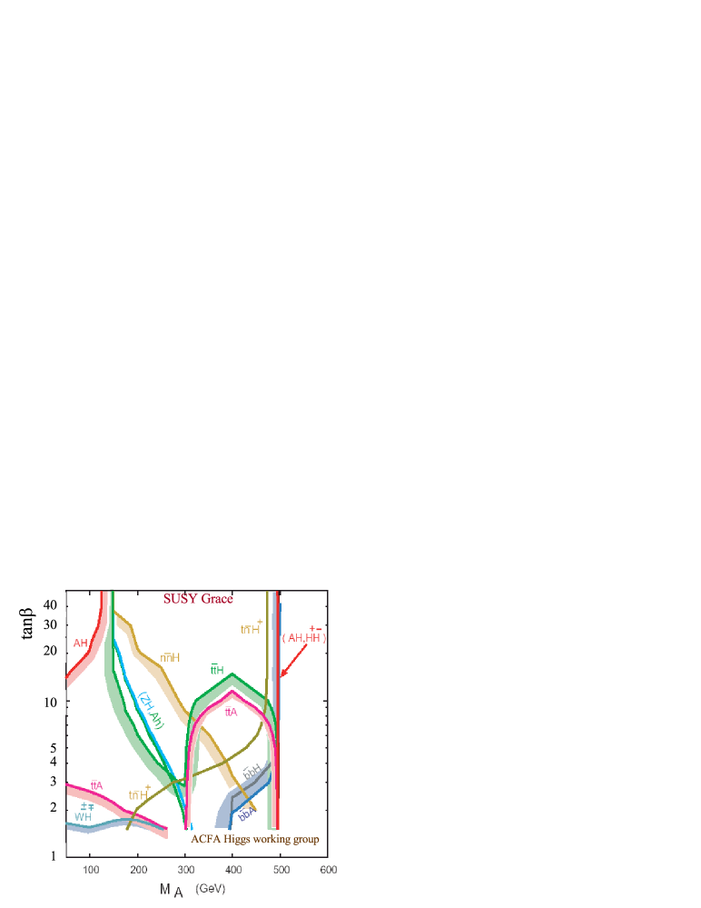
Figure 9: Visibility of heavy SUSY Higgses at ILC ($\sqrt{s}=1{\,\mathrm{Te\kern-1.00006ptV}}$).

In addition to the direct searches the precision branching ratio measurements of the light Higgs can give indications of the H and A mass. Figure 10 shows the ratio of branching ratios $BR(h\rightarrow{\mathrm{b}\bar{\mathrm{b}}})/BR(h\rightarrow WW)$ of the MSSM relative to the Standard Model as a function of $m_{\mathrm{H}}$[18]. The width of the band gives the uncertainty from the measurement of the MSSM parameters. Up to A masses of a few hundred GeV one can get a good indication of $m_{\mathrm{A}}$.

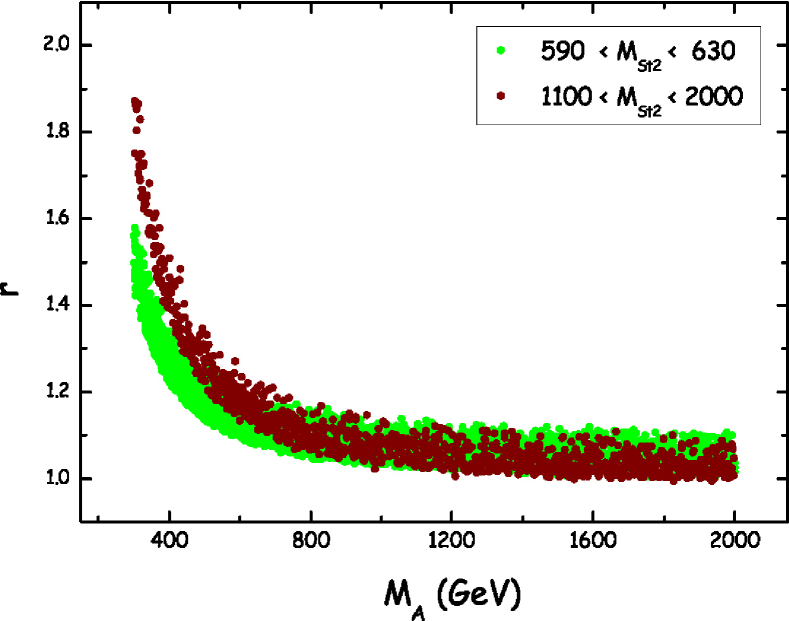
Figure 10: $BR(h\rightarrow{\mathrm{b}\bar{\mathrm{b}}})/BR(h\rightarrow WW)$ MSSM/SM within the SPS1a scenario as a function of $m_{\mathrm{A}}$.

Another possibility to find the heavy SUSY Higgses is the photon collider. Since Higgses are produced in the s-channel the maximum reach is twice the beam energy corresponding to $0.8\sqrt{s}_{ee}$. Figure 11 shows the expected sensitivity in one year of running for $m_{\mathrm{A}}=350{\,\mathrm{Ge\kern-1.00006ptV}}$, $\sqrt{s}_{ee}=500{\,\mathrm{Ge\kern-1.00006ptV}}$ and different SUSY parameters[19]. In general H and A are clearly visible, however due to the loop coupling of the $\gamma$ to the Higgs the sensitivity becomes model dependent.

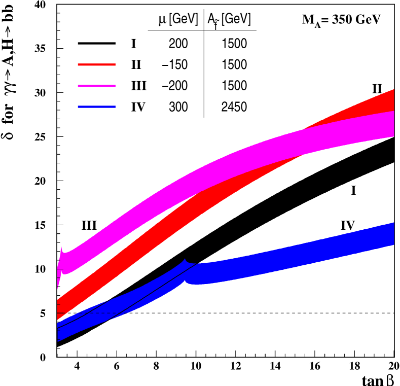
Figure 11: Sensitivity of the $\gamma\gamma$ collider to heavy MSSM Higgses. ($m_{\mathrm{A}}=350{\,\mathrm{Ge\kern-1.00006ptV}}$, $\sqrt{s}_{ee}=500{\,\mathrm{Ge\kern-1.00006ptV}}$, $M_{2}=200{\,\mathrm{Ge\kern-1.00006ptV}}$, $M_{\tilde{f}}=1000{\,\mathrm{Ge\kern-1.00006ptV}}$)

4 Supersymmetry and Dark Matter

Supersymmetry (SUSY) is the best motivated extension of the Standard Model. Up to now all data are consistent with SUSY, however also with the pure Standard Model. Contrary to the SM, SUSY allows the unification of couplings at the GUT scale and, if R-parity is conserved, SUSY offers a perfect dark matter candidate. If some superpartners are visible at the ILC they will be discovered by the LHC in most part of the parameter space. However many tasks are left for the ILC in this case. First the ILC has to confirm that the discovered new states are really superpartners of the Standard Model particles. Then it has to measure as many of the $>100$ free parameters as possible in a model independent way which allows to check if grand unification works and to get an idea by which mechanism Supersymmetry is broken. If Supersymmetric particles are a source of dark matter the ILC has to measure their properties.

Within the minimal supergravity model (mSUGRA) the parameter space can be strongly restricted requiring that the abundance of the lightest neutralino, which is stable in this model, is consistent with the dark matter density measured by WMAP. Figure 12 shows the allowed region in a pictorial way[20]. In the so called “bulk region” all superpartners are light and many are visible at the LHC and the ILC. In the “coannihilation region” the mass difference between the lightest neutralino, $\tilde{\chi}^{0}_{1}$, and the lighter stau, $\tilde{\tau}_{1}$, is very small so that the $\tilde{\tau}_{1}$-decay particles that are visible by the detector have only a very small momentum. In the “focus point region” the $\tilde{\chi}^{0}_{1}$ gets a significant Higgsino component enhancing its annihilation cross section. This leads to relatively heavy scalars, probably invisible at the ILC and the LHC. Other regions, like the “rapid annihilation funnel” are characterised by special resonance conditions, like $2m(\tilde{\chi}^{0}_{1})\approx m_{\mathrm{A}}$, increasing the annihilation rate. All these special regions tend to be challenging for both machines.

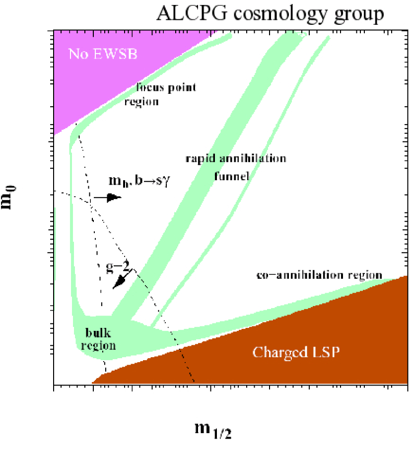
Figure 12: Dark matter allowed regions of mSUGRA.

After new states consistent with SUSY have been discovered at the LHC, the ILC can check, if it is really Supersymmetry. As an example fig. 13 shows the threshold behaviour of smuon production and the production of Kaluza Klein excitations of the muon[21]. There is no problem for the ILC to distinguish the two possibilities. Figure 14 shows the expected precision of the measurement of the SU(2) and U(1) coupling of the selectron[22]. The agreement with the couplings of the electron can be tested to the percent to per mille level.

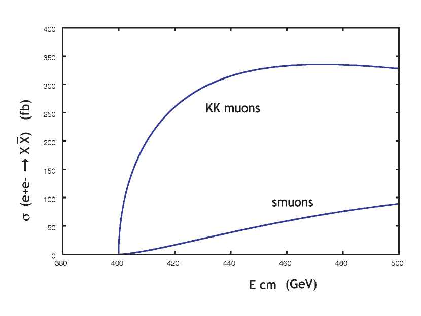
Figure 13: Threshold behaviour of smuon production and the production of Kaluza Klein excitations of the muon.

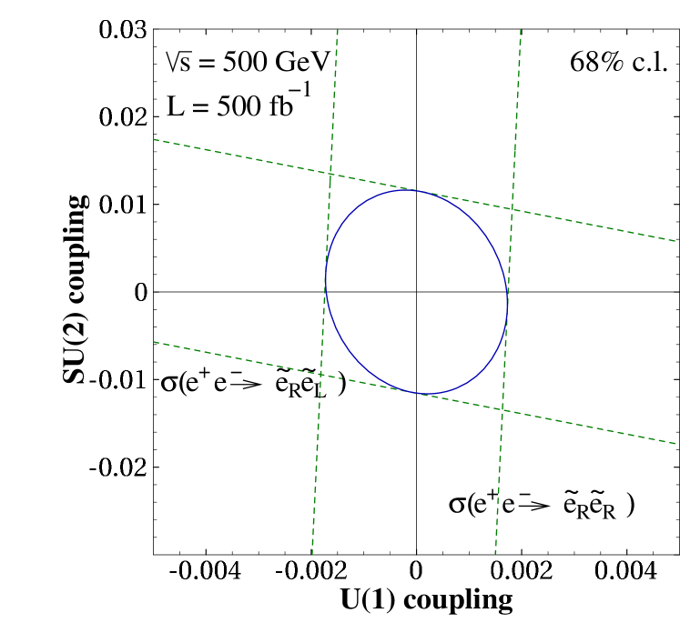
Figure 14: Measurement of the SU(2) and U(1) coupling of the selectron at the ILC.

4.1 SUSY in the bulk region

An often studied benchmark point in the bulk region is the SPS1a scenario[23]. In this scenario all sleptons, neutralinos and charginos are visible at ILC and and in addition squarks and gluinos at the LHC. The LHC can measure mass differences pretty accurately, but has difficulties to measure absolute masses. The ILC, however can measure absolute masses with good precision, including the one of the $\tilde{\chi}^{0}_{1}$. Table 1 shows the expected precision for the mass measurements for the LHC and ILC alone and for the combination[24]. In many cases the combination is significantly better than the LHC or even the ILC alone. As an example figure 15 shows the correlation between the squark mass and the $\tilde{\chi}^{0}_{1}$ mass from LHC together with $m(\tilde{\chi}^{0}_{1})$ from ILC[24]. The improvement in $m(\tilde{q})$ is evident.

	$m_{\rm SPS1a}$	LHC	ILC	LHC+ILC		$m_{\rm SPS1a}$	LHC	ILC	LHC+ILC
$h$	111.6	0.25	0.05	0.05	$H$	399.6		1.5	1.5
$A$	399.1		1.5	1.5	$H+$	407.1		1.5	1.5
$\chi_{1}^{0}$	97.03	4.8	0.05	0.05	$\chi_{2}^{0}$	182.9	4.7	1.2	0.08
$\chi_{3}^{0}$	349.2		4.0	4.0	$\chi_{4}^{0}$	370.3	5.1	4.0	2.3
$\chi^{\pm}_{1}$	182.3		0.55	0.55	$\chi^{\pm}_{2}$	370.6		3.0	3.0
$\tilde{g}$	615.7	8.0		6.5
$\tilde{t}_{1}$	411.8		2.0	2.0
$\tilde{b}_{1}$	520.8	7.5		5.7	$\tilde{b}_{2}$	550.4	7.9		6.2
$\tilde{u}_{1},\tilde{c}_{1}$	551.0	19.0		16.0	$\tilde{u}_{2},\tilde{c}_{2}$	570.8	17.4		9.8
$\tilde{d}_{1},\tilde{s}_{1}$	549.9	19.0		16.0	$\tilde{d}_{2},\tilde{s}_{2}$	576.4	17.4		9.8
$\tilde{e}_{1}$	144.9	4.8	.05	0.05	$\tilde{e}_{2}$	204.2	5.0	0.2	0.2
$\tilde{\mu}_{1}$	144.9	4.8	0.2	0.2	$\tilde{\mu}_{2}$	204.2	5.0	0.5	0.5
$\tilde{\tau}_{1}$	135.5	6.5	0.3	0.3	$\tilde{\tau}_{2}$	207.9		1.1	1.1
$\tilde{\nu}_{e}$	188.2		1.2	1.2

Table 1: Expected precision of mass measurements at LHC and ILC in the SPS1a scenario.

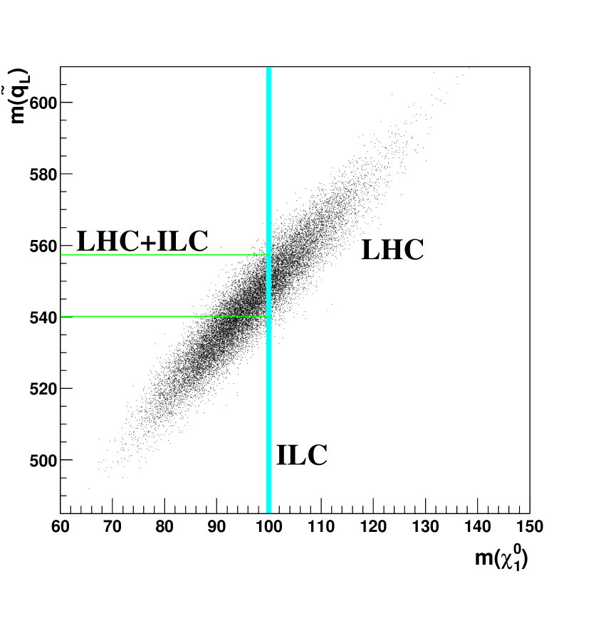
Figure 15: Correlation between $m(\tilde{\chi}^{0}_{1})$ and $m(\tilde{q})$ measurements at LHC together with $m(\tilde{\chi}^{0}_{1})$ from ILC.

With these inputs it is then possible to fit many of the low energy SUSY breaking parameters in a model independent way. Figure 16 shows the result of this fit to the combined ILC and LHC results for the SPS1a scenario[25]. Most parameters can be measured on the percent level.

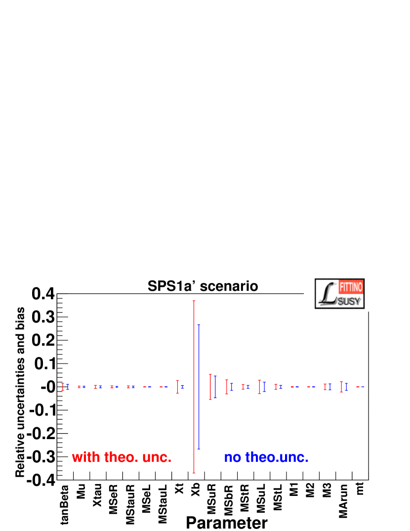
Figure 16: Low energy SUSY breaking parameters from a fit to the LHC and ILC results.

These parameters can then be extrapolated to high scales using the renormalisation group equations to check grand unification[26]. Figure 17 shows the expected precision for the gaugino and slepton mass parameters and for the coupling constants.

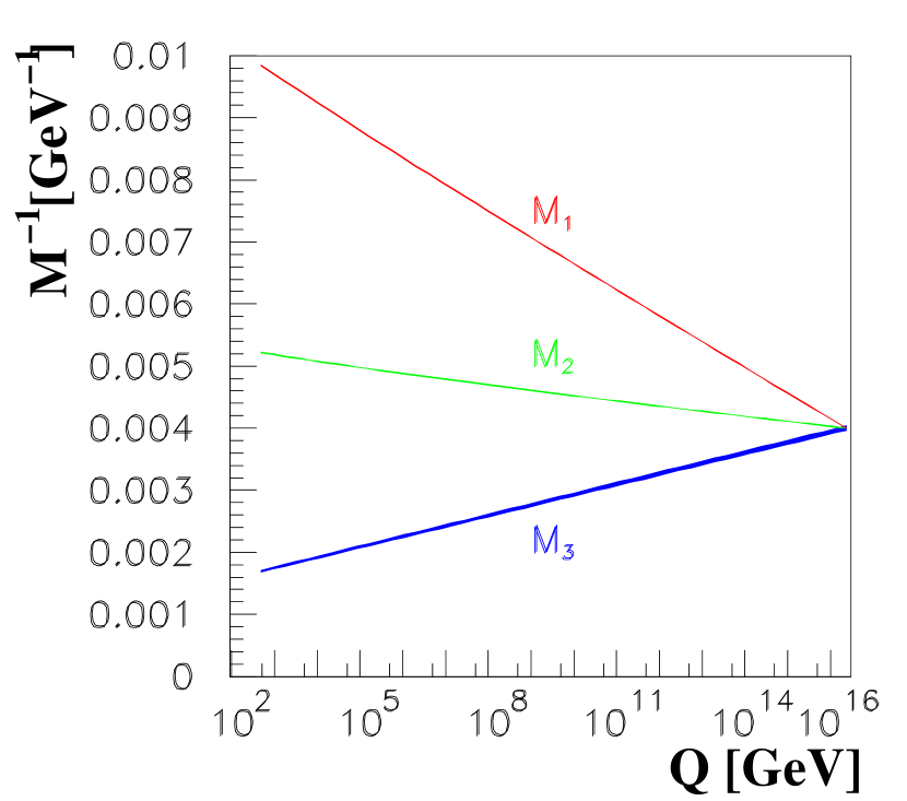
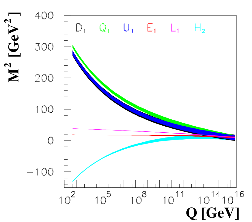
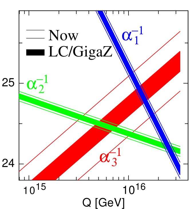
Figure 17: Extrapolation of the gaugino and slepton mass parameters and of the coupling constants to the GUT scale.

4.2 Reconstruction of dark matter

As already mentioned the lightest neutralino is a good candidate for the dark matter particle. To calculate its density in the universe, the properties of all particles contributing to the annihilation have to be reconstructed with good precision. In any case the mixing angles and mass of the $\tilde{\chi}^{0}_{1}$ need to be known. However also the properties of other particles can be important. For example in the $\tilde{\chi}^{0}_{1}-\tilde{\tau}_{1}$ coannihilation region the $\tilde{\chi}^{0}_{1}-\tilde{\tau}_{1}$ mass difference is essential. Figure 18 shows the possible precision with which the dark matter density and neutralino mass can be reconstructed from the LHC and the ILC measurements[27]. ILC matches nicely the expected precision of the Planck satellite, allowing a stringent test whether Supersymmetry can account for all dark matter in the universe.

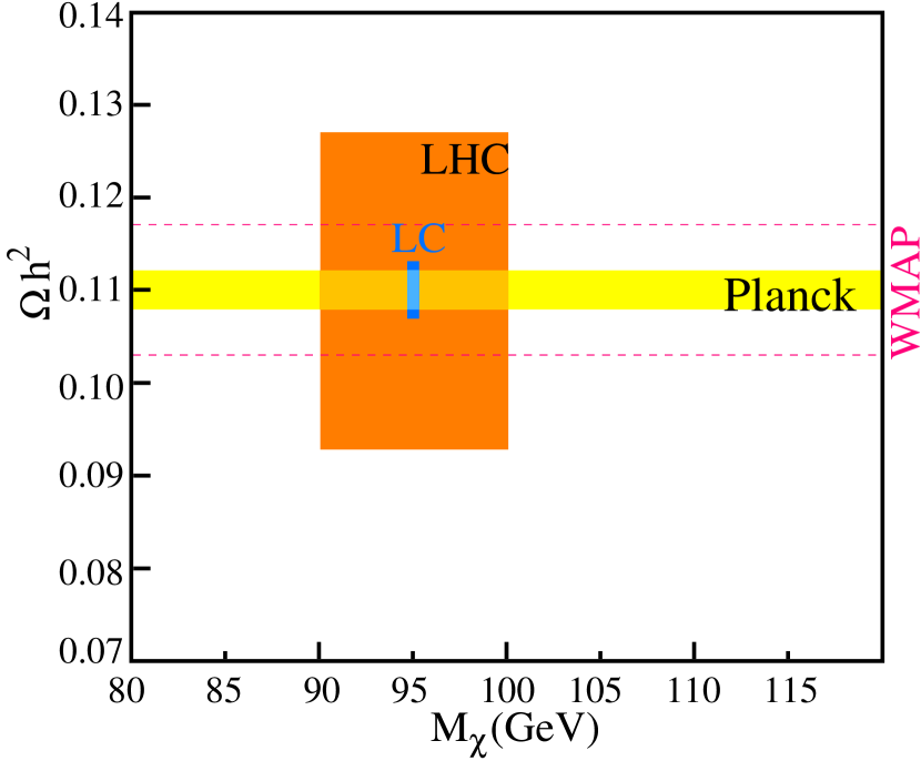
Figure 18: Projected precision of the dark matter density in the coannihilation region from WMAP, Planck, LHC and ILC.

5 Models without a Higgs

Without a Higgs WW scattering becomes strong at high energy, finally violating unitarity at 1.2 TeV. One can thus expect new physics the latest at this scale. At the moment there are mainly two classes of models that explain electroweak symmetry breaking without a Higgs boson. In Technicolour like models[28] new strong interactions are introduced at the TeV scale. In Higgsless models the unitarity violation is postponed to higher energy by new gauge bosons, typically KK excitations of the Standard Model gauge bosons. Both classes should give visible signals at the ILC. The accessible channels are W-pair production, where the exchanged $\gamma$ or Z may fluctuate into a new state, vector boson scattering, where the new states can be exchanged in the s- or t-channel of the scattering process and three gauge boson production where the new states can appear in the decay of the primary $\gamma$ or Z.

5.1 Strong electroweak symmetry breaking

As already said, in technicolour like models one expects new strong interactions, including resonances, at the TeV scale. To analyse these models in a model independent way, the triple and quartic couplings can be parameterised by an effective Lagrangian in a dimensional expansion[29]. For the interpretation the effects of resonances on these couplings can then be calculated. Figure 19 shows the possible sensitivity to $\alpha_{4}$ and $\alpha_{5}$ at $\sqrt{s}=1{\,\mathrm{Te\kern-1.00006ptV}}$ from vector-boson scattering and three vector boson production[30]. Typical sensitivities are ${\cal O}(0.1/16\pi^{2})$ for triple and ${\cal O}(1/16\pi^{2})$ for quartic couplings. This corresponds to mass limits around $3{\,\mathrm{Te\kern-1.00006ptV}}$ for maximally coupled resonances. The different processes can then distinguish between the different resonances. For example W-pair production is only sensitive to vector resonances.

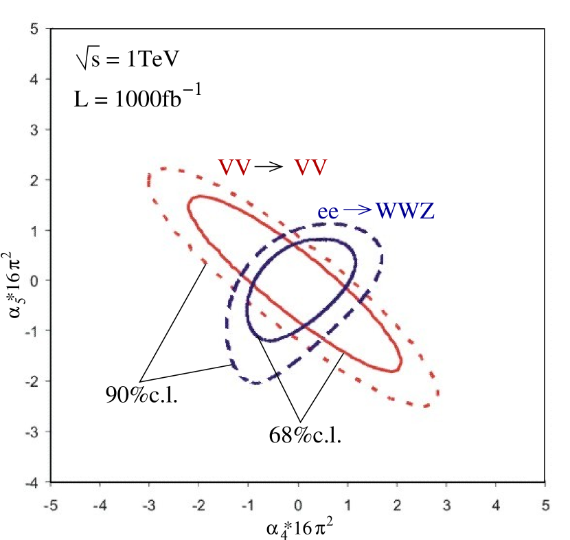
Figure 19: Expected sensitivity on $\alpha_{4}$ and $\alpha_{5}$ from vector boson scattering and three vector boson production.

5.2 Higgsless models

Higgsless models predict new gauge bosons at higher energies. Especially also charged states are predicted that cannot be confused with a heavy Higgs. Figure 20 shows the cross section for the process $WZ\rightarrow WZ$ in a Higgsless model, the Standard Model without a Higgs and the SM where unitarity is restored by a 600 GeV Higgs[31, 32]. Detailed studies show that these states can be seen at LHC, however it is out of question that such a state would also give a signal at ILC in $WZ\rightarrow WZ$ and in $WWZ$ production so that its properties could be measured in detail.

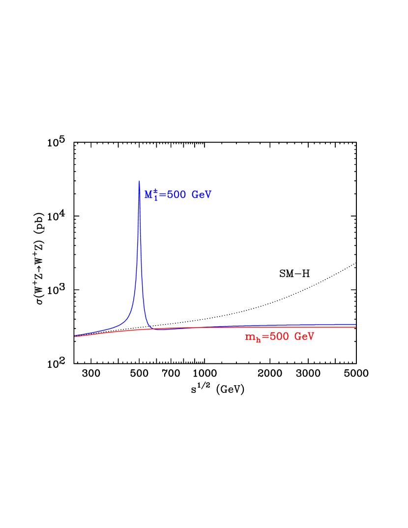
Figure 20: Cross section $\sigma(WZ\rightarrow WZ)$ in a Higgsless model and in the Standard Model with and without a Higgs[32].

6 Extra Gauge Bosons

The ILC is sensitive to new gauge bosons in $\mathrm{e}^{+}\mathrm{e}^{-}\rightarrow{\rm f}\overline{\rm f}$ via the interference with the Standard Model amplitude far beyond $\sqrt{s}$. The sensitivity is typically even larger than at the LHC. If the LHC measures the mass of a new Z’ a precise coupling measurement is possible at the ILC. In addition angular distributions are sensitive to the spin of the new state and can thus distinguish for example between a Z’ and KK graviton towers. A review of the sensitivity can be found in[11].

An interesting possibility is the reconstruction of the 2nd excitation of the Z and $\gamma$ in universal extra dimensions. In this models an excitation quantum number may be defined that is conserved and makes the lightest excitation stable and thus a good dark matter candidate[33]. The second excitations couple to Standard Model particles only loop suppressed and thus weakly[34]. Cosmology suggests $\frac{1}{R}\approx m(\gamma^{\prime})<1{\,\mathrm{Te\kern-1.00006ptV}}$ corresponding to $m(\gamma^{\prime\prime})<2{\,\mathrm{Te\kern-1.00006ptV}}$[33]. The LHC can see the $\gamma^{\prime}$ in pair production up to about this energy. The ILC is sensitive to the $Z^{\prime\prime}$ and $\gamma^{\prime\prime}$ up to $2\sqrt{s}$ which corresponds to the same $1/R$ reach for $\sqrt{s}=1{\,\mathrm{Te\kern-1.00006ptV}}$ (see fig. 21)[35], helping enormously in the interpretation of a possible LHC signal as KK excitation.

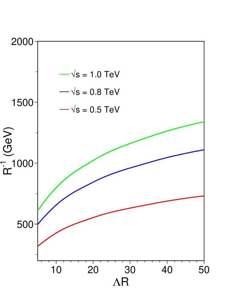
Figure 21: ILC reach for the $Z^{\prime\prime},\,\gamma^{\prime\prime}$ expressed in $1/R$ as a function of the cutoff parameter $\Lambda R$[35]. A $\Lambda R$ value around 30 is suggested theoretically[34].

Little Higgs models explain the “little hierarchy problem” by a new gauge structure and a new top-like quark[36]. The new gauge structure also predicts new vector bosons ($Z_{H},\,A_{H},\,W_{H}$) at masses of a few TeV. Figure 22 shows the precision with which the mixing angles of the $Z_{H}$ can be measured at $\sqrt{s}=500{\,\mathrm{Ge\kern-1.00006ptV}}$ once its mass ($3.3{\,\mathrm{Te\kern-1.00006ptV}}$ in this example) in measured at the LHC[37].

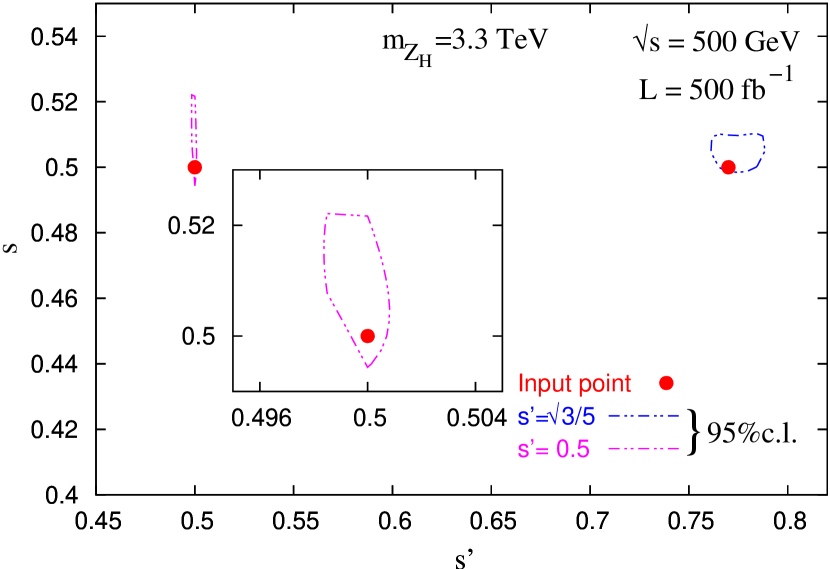
Figure 22: Measurement of the $Z_{H}$ mixing angles at the ILC.

7 Conclusions

Independent of which physics scenario nature has chosen, the ILC will be needed in addition to the LHC. If there is a Higgs and SUSY the ILC has to reconstruct as many of the SUSY-breaking parameters as possible, extrapolate them to the GUT scale to get some understanding of the breaking mechanism and measure the properties of the dark matter particle.

If there is a Higgs without Supersymmetry the precision measurements of the Higgs boson guide the way to the model of electroweak symmetry breaking. In addition several models, like some extra dimension models or little Higgs models have extra gauge bosons that are visible via their indirect effects.

If the LHC doesn’t find any Higgs boson, the ILC can fill some loopholes that still exist, can see signals of strong electroweak symmetry breaking and is sensitive to a new gauge sector.

In any case we know that the top quark is accessible to the ILC and that its properties can be measured with great precision.

DISCUSSION

Bernd Jantzen

(Univ. of Karlsruhe): Can anything be said about if we need CLIC and what we would like to explore with it before the data of LHC and/or ILC has been analysed?

Klaus Mönig:

The detailed physics case for CLIC can only be made once we know the scenario realised in nature. For example if relatively light SUSY exists CLIC can extend the ILC precision measurements to the coloured part of the spectrum. However, it may also be possible, that a hadron collider at very high energy may be the better next machine at the energy frontier.

References

-
[1]
Understanding Matter, Energy, Space and Time: the
Case for the Linear Collider,
http://sbhep1.physics.sunysb.edu/~grannis/lc_consensus.html - [2] J. Dorfan, these proceedings.
- [3] F. Zimmermann, these proceedings.
- [4] G. Rolandi, these proceedings.
- [5] F. Gianotti, these proceedings.
- [6] A. H. Hoang et al., Phys. Rev. D 65 (2002) 014014 [arXiv:hep-ph/0107144].
- [7] M. Martinez and R. Miquel, Eur. Phys. J. C 27 (2003) 49 [arXiv:hep-ph/0207315].
- [8] S. Heinemeyer, S. Kraml, W. Porod and G. Weiglein, JHEP 0309 (2003) 075 [arXiv:hep-ph/0306181].
- [9] J. R. Ellis, S. Heinemeyer, K. A. Olive and G. Weiglein, JHEP 0502 (2005) 013 [arXiv:hep-ph/0411216].
- [10] J.C.Brient, private communication
-
[11]
J. A. Aguilar-Saavedra et al.,
TESLA Technical Design Report Part III: Physics at an Linear Collider, DESY-01-011C. - [12] A.Gay, talk presented at LCWS04, Paris, April 2004.
- [13] S.Yamashita talk presented at the 7th ACFA workshop, Taipei, November 2004.
- [14] S. Kanemura, Y. Okada and E. Senaha, arXiv:hep-ph/0507259.
- [15] K. Mönig and A. Rosca, arXiv:hep-ph/0506271.
- [16] P. Niezurawski, A. F. Zarnecki and M. Krawczyk, arXiv:hep-ph/0307183.
- [17] T. Han, H. E. Logan, B. McElrath and L. T. Wang, Phys. Lett. B 563 (2003) 191 [Erratum-ibid. B 603 (2004) 257] [arXiv:hep-ph/0302188].
- [18] K. Desch, E. Gross, S. Heinemeyer, G. Weiglein and L. Zivkovic, JHEP 0409 (2004) 062 [arXiv:hep-ph/0406322].
- [19] P. Niezurawski, A. F. Zarnecki and M. Krawczyk, arXiv:hep-ph/0507006.
- [20] J. L. Feng, arXiv:hep-ph/0509309.
- [21] M. Peskin, talk at the ALPG meeting, Victoria, Canada, July 2004.
- [22] A. Freitas, A. von Manteuffel and P. M. Zerwas, Eur. Phys. J. C 34 (2004) 487 [arXiv:hep-ph/0310182].
- [23] B. C. Allanach et al., Eur. Phys. J. C25 (2002) 113.
-
[24]
G. Weiglein et al.
arXiv:hep-ph/0410364. - [25] P. Bechtle, K. Desch and P. Wienemann, arXiv:hep-ph/0506244.
- [26] B. C. Allanach et al., Nucl. Phys. Proc. Suppl. 135 (2004) 107 [arXiv:hep-ph/0407067].
- [27] M. Berggren, F. Richard and Z. Zhang, LAL 05-104, arXiv:hep-ph/0510088.
- [28] C. T. Hill and E. H. Simmons, Phys. Rept. 381 (2003) 235 [Erratum-ibid. 390 (2004) 553] [arXiv:hep-ph/0203079].
- [29] W. Kilian and J. Reuter, arXiv:hep-ph/0507099.
-
[30]
P. Krstonosic et al.,
arXiv:hep-ph/0508179. - [31] A. Birkedal, K. Matchev and M. Perelstein, Phys. Rev. Lett. 94 (2005) 191803 [arXiv:hep-ph/0412278].
- [32] A. Birkedal, K. T. Matchev and M. Perelstein, arXiv:hep-ph/0508185.
- [33] G. Servant and T. M. P. Tait, Nucl. Phys. B 650, 391 (2003) [arXiv:hep-ph/0206071].
- [34] H. C. P. Cheng, K. T. Matchev and M. Schmaltz, Phys. Rev. D 66, 036005 (2002) [arXiv:hep-ph/0204342].
- [35] S. Riemann, arXiv:hep-ph/0508136.
- [36] N. Arkani-Hamed, A. G. Cohen and H. Georgi, Phys. Lett. B 513 (2001) 232 [arXiv:hep-ph/0105239].
- [37] J. A. Conley, J. Hewett and M. P. Le, arXiv:hep-ph/0507198.