More on a possible energy dependence of $\Theta_{13}$ in vacuum neutrino oscillations

Abstract

Vacuum neutrino-oscillation probabilities from a simple three-flavor model with both mass-square differences and timelike Fermi-point splittings have been presented in a previous article [hep-ph/0504274]. Here, further results are given: first, for specific parameters relevant to MINOS in the low-energy mode and, then, for arbitrary parameters. A generalized model with equidistant Fermi-point splittings and an additional complex phase is also discussed. If relevant, this generalized model might have interesting effects at future long-baseline oscillation experiments.

I Introduction

In a previous article KlinkhamerTheta13 , we have considered a simple three-flavor neutrino-oscillation model with both mass-square differences ($\Delta m^{2}_{ij}$) and timelike Fermi-point splittings ($\Delta b_{0}^{(ij)}$). The mixing of the mass sector is taken to be bi-maximal and the one of the Fermi-point-splitting sector trimaximal, with all complex phases vanishing. The model has furthermore a hierarchy of Fermi-point splittings ($b_{0}^{(1)}=b_{0}^{(2)}\neq b_{0}^{(3)}$) which parallels the hierarchy of masses ($m_{1}=m_{2}\neq m_{3}$). This particular model may be called the “stealth model,” as it allows for Lorentz-noninvariant Fermi-point-splitting effects to hide behind mass-difference effects. For the physics motivation of this type of model discussion, see Ref. KlinkhamerTheta13 and references therein.

The present article follows up the previous one in three ways. First, we give model results of the vacuum appearance probability $P(\nu_{\mu}\rightarrow\nu_{e})$ relevant to MINOS in the low-energy mode, complementing the specific results for the medium energy mode in Ref. KlinkhamerTheta13 .

Second, we consider the model probability $P_{\mu e}\equiv P(\nu_{\mu}\rightarrow\nu_{e})$ for the case of relatively strong Fermi-point-splitting effects compared to mass-difference effects, whereas Ref. KlinkhamerTheta13 focused on relatively weak splitting effects. In particular, we introduce a new parametrization (with nonnegative dimensionless parameters $\rho$ and $\tau$) which makes a straightforward comparison between different long-baseline neutrino-oscillation experiments possible. Relatively weak or strong Fermi-point-splitting effects then correspond to $\rho\tau\ll 1$ or $\rho\tau\gtrsim 1$, respectively. The behavior of $P_{\mu e}(\rho,\tau)$ turns out to be quite complicated for $\rho\tau\gtrsim 1$,

Third, we present results on the appearance probability $P(\nu_{\mu}\rightarrow\nu_{e})$ from a generalized model with the same mass hierarchy as the model of Ref. KlinkhamerTheta13 but with equidistant Fermi-point splittings ($\,b_{0}^{(2)}-b_{0}^{(1)}=b_{0}^{(3)}-b_{0}^{(2)}\,$) and one additional complex phase ($\omega=\pi/4$). For completeness, we also give the model probability of the time-reversed process, $\nu_{e}\rightarrow\nu_{\mu}$. It will be seen that the generalized model has a rather interesting phenomenology with stealth-like characteristics in certain cases and strong time-reversal noninvariance in others.

The outline for the remainder of this article is as follows. In Sec. II, we recall the definition of the model and introduce the two neutrino-oscillation parameters $\rho$ and $\tau$. In Sec. III, we present and discuss our new results. In the Appendix, we consider one concrete model and compare the capabilities of four accelerator-based long-baseline oscillation experiments.

II Model

Setting $\hbar=c=1$ and writing $p\equiv|\vec{p}\,|$ for the neutrino momentum, the Hamiltonian of the stealth model KlinkhamerTheta13 contains three terms in the $(\nu_{e},\nu_{\mu},\nu_{\tau})$ flavor basis,

$$H\supset p\,\openone+X\cdot D_{m}\cdot X^{-1}+Y\cdot D_{b_{0}}\cdot Y^{-1}\,,$$ (1)

with diagonal matrices

$$D_{m}\equiv\mathrm{diag}\left(\,\frac{m^{2}_{1}}{2p}\,,\,\frac{m^{2}_{2}}{2p}\,,\,\frac{m^{2}_{3}}{2p}\,\right)\,,\quad D_{b_{0}}\equiv\mathrm{diag}\left(\,b_{0}^{(1)}\,,\,b_{0}^{(2)}\,,\,b_{0}^{(3)}\,\right)\,,$$ (2)

and $SU(3)$ matrices

$$X \equiv M_{32}(\theta_{32})\cdot M_{13}(\theta_{13},\delta)\cdot M_{21}(\theta_{21})\,,\quad Y\equiv M_{32}(\chi_{32})\cdot M_{13}(\chi_{13},\omega)\cdot M_{21}(\chi_{21})\,,$$ (3)

in terms of the basic matrices

$$M_{32}(\vartheta) \equiv \left(\begin{array}[]{ccc}1&\;\;\;0&0\\ 0&\;\;\;\cos\vartheta&\sin\vartheta\\ 0&\;\;\;-\sin\vartheta&\cos\vartheta\end{array}\right)\,,\quad M_{21}(\vartheta)\equiv\left(\begin{array}[]{ccc}\cos\vartheta&\;\;\;\sin\vartheta&0\\ -\sin\vartheta&\;\;\;\cos\vartheta&0\\ 0&0&1\end{array}\right)\,,$$ (10)

$$M_{13}(\vartheta,\varphi) \equiv \left(\begin{array}[]{ccc}\cos\vartheta&\;\;\;0&\;+e^{+i\varphi}\,\sin\vartheta\\ 0&\;\;\;1&0\\ -e^{-i\varphi}\,\sin\vartheta&\;\;\;0&\cos\vartheta\end{array}\right)\,,$$ (14)

and the following parameters:

$$\Delta m^{2}_{21} \equiv m_{2}^{2}-m_{1}^{2}=0\,,\quad R\equiv\Delta b_{0}^{(21)}/\Delta b_{0}^{(32)}\equiv(b_{0}^{(2)}-b_{0}^{(1)})/(b_{0}^{(3)}-b_{0}^{(2)})=0\,,$$ (15a)

$$\theta_{13} = 0\,,\quad\theta_{21}=\theta_{32}=\chi_{13}=\chi_{21}=\chi_{32}=\pi/4\,,$$ (15b)

$$\delta = \omega=0\,.$$ (15c)

With all other complex phases vanishing, there are only two neutrino-oscillation parameters left in the model,

$$\Delta m^{2}_{31}\equiv m_{3}^{2}-m_{1}^{2}>0\,,\quad\Delta b_{0}^{(31)}\equiv b_{0}^{(3)}-b_{0}^{(1)}>0\,,$$ (16)

which have been taken positive.

For high-energy neutrino oscillations over a travel distance $L$, there are, then, two dimensionless parameters which completely define the problem, at least for the simple model considered and matter effects neglected. These neutrino-oscillation parameters can be defined as follows ($E_{\nu}\sim p$):

$$\rho \equiv \frac{{2\,E_{\nu}\,\hbar c}_{\vphantom{!_{a}}}}{{|\Delta m^{2}_{31}|\,c^{4}\,L}^{\vphantom{a}}}\approx\left(\frac{{2.5\times 10^{-3}\;\mathrm{eV}^{2}/c^{4}}_{\vphantom{!_{a}}}}{{|\Delta m^{2}_{31}|}^{\vphantom{a}}}\right)\,\left(\frac{{735\;\mathrm{km}}_{\vphantom{!_{a}}}}{{L}^{\vphantom{a}}}\right)\,\left(\frac{{E_{\nu}}_{\vphantom{!_{a}}}}{{4.656\;\mathrm{GeV}}^{\vphantom{a}}}\right)\,,$$ (17a)

$$\newline \tau \equiv \frac{{L\,|\Delta b_{0}^{(31)}|}_{\vphantom{!_{a}}}}{{\hbar c}^{\vphantom{a}}}\approx\left(\frac{{|\Delta b_{0}^{(31)}|}_{\vphantom{!_{a}}}}{{2.685\times 10^{-13}\;\mathrm{eV}}^{\vphantom{a}}}\right)\,\left(\frac{{L}_{\vphantom{!_{a}}}}{{735\;\mathrm{km}}^{\vphantom{a}}}\right)\,,$$ (17b)

with $\hbar$ and $c$ temporarily reinstated.

In terms of these parameters, an approximate formula for the vacuum probability $P_{\mu e}\equiv P(\nu_{\mu}\rightarrow\nu_{e})$ is given by KlinkhamerTheta13

$$P_{\mu e}^{\mathrm{\,stealth}}(\rho,\tau)\sim(1/2)\,\sin^{2}(2\,\Theta_{13})\;\sin^{2}\left(\left[\>\rho^{-1}+\tau+\sqrt{\rho^{-2}+\tau^{2}}\;\right]/4\,\right)\,,$$ (18a)

with the following energy-dependent effective mixing angle:

$$\Theta_{13}(\rho,\tau)\sim(1/2)\,\arctan(\rho\,\tau)\,.$$ (18b)

Recall that, according to Eq. (15b), the bare mixing angle $\theta_{13}$ vanishes identically and that, as mentioned above, matter effects are neglected in this approximate model probability endnote-matter .

More generally and allowing for a nonzero Fermi-point-splitting ratio $R$, one can define

$$P_{\mu e}^{\mathrm{\,stealth}}(\rho,\tau)=\sin^{2}(\widehat{\Theta}_{32})\,\sin^{2}(2\,\widehat{\Theta}_{13})\;\widehat{\Lambda}_{\mu e}^{\,2}\,,$$ (19a)

with the following functional dependence:

$$\widehat{\Theta}_{32}=\widehat{\Theta}_{32}(\rho\,\tau\,,R)\,,\quad\widehat{\Theta}_{13}=\widehat{\Theta}_{13}(\rho\,\tau\,,R)\,,\quad\widehat{\Lambda}_{\mu e}=\widehat{\Lambda}_{\mu e}(\rho\,,\,\tau\,,R)\in[-1,+1]\,,$$ (19b)

so that the effective mixing angles $\widehat{\Theta}_{32}$ and $\widehat{\Theta}_{13}$ are independent of the travel distance $L$, according to Eqs. (17ab), whereas $\widehat{\Lambda}_{\mu e}$ does depend on $L$ endnote-Lambdahat . In principle, $\widehat{\Theta}_{13}$ does not have to vanish in the limit $\rho\to 0$ for fixed $\tau$ and this is indeed the case for the generalized model with splitting ratio $R\neq 0$ (see below).

III Results and discussion

In Ref. KlinkhamerTheta13 , we have given five figures with model results, three of which may be relevant to T2K or NO$\nu$A and two to MINOS in the medium-energy (ME) mode. Here, we present one more figure, Fig. 1, which may be relevant to MINOS (baseline $L=735\;\mathrm{km}$) in the low-energy (LE) mode, with peak neutrino energy $\overline{E}_{\nu}$ approximately equal to $3.75\;\mathrm{GeV}$ and neutrino-oscillation length scale $\overline{L}\equiv 2\pi\overline{E}_{\nu}/|\Delta m^{2}_{31}|\approx 1860\;\mathrm{km}$ for $\Delta m^{2}_{31}=2.5\times 10^{-3}\;\mathrm{eV}^{2}$. Figure 1 (which may be compared to Figs. 4 and 5 of Ref. KlinkhamerTheta13 ) shows that, if MINOS–LE would be able to place an upper limit of $10\,\%$ on the appearance probability $P(\nu_{\mu}\rightarrow\nu_{e})$ at the high end of the energy spectrum ($E_{\nu}\gtrsim 4\;\mathrm{GeV}$), this would correspond to an upper limit on $|\Delta b_{0}^{(31)}|$ of approximately $3\times 10^{-13}\;\mathrm{eV}$ (assuming $\tau\leq\pi$, see below).

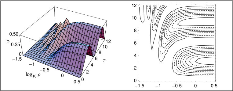
Figure 2: Numerical results for the vacuum probability $P_{\mu e}\equiv P(\nu_{\mu}\rightarrow\nu_{e})$ from the “stealth” model (1)–(16), as a function of the two dimensionless parameters $\rho$ and $\tau$, defined by Eqs. (17ab). Left: surface plot. Right: contour plot, with equidistant contours at $P_{\mu e}=0.05,0.10,0.15,\ldots\,0.45$ and contours at integer multiples of 0.10 shown dashed.

A further figure, Fig. 2, gives numerical results which illustrate the general behavior of the vacuum probability $P_{\mu e}\equiv P(\nu_{\mu}\rightarrow\nu_{e})$ as a function of the two dimensionless parameters $\rho$ and $\tau$ from Eqs. (17ab). Note that we expect $\lim_{\tau\to 0}P_{\mu e}(\rho,\tau)$ to vanish [pure mass-difference model with $\Delta m^{2}_{21}=0$ and $\theta_{13}=0$] and $\lim_{\rho\to\infty}P_{\mu e}(\rho,\tau)$ to be given by $(1/2)\,\sin^{2}(\tau/2)$ [pure Fermi-point-splitting model with $\Delta b_{0}^{(21)}=0$, $\Delta b_{0}^{(31)}\neq 0$, and trimaximal mixing]. The landscape of Fig. 2 can then be described as follows: mountain ridges start out at $\rho\gg 1$ and $\tau\approx n_{\infty}\,\pi$ for odd integers $n_{\infty}$, slope down towards lower values of $\rho$ keeping approximately the same values of $\tau$, and, finally, disappear while bending towards lower values of $\tau$ (more so for ridges with large $n_{\infty}$). This topography is qualitatively reproduced by the analytic expression (18).

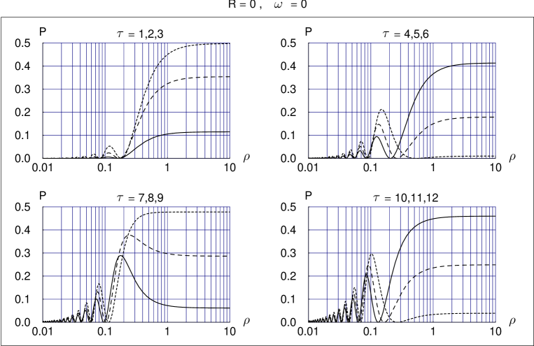
Figure 3: Numerical results for constant–$\tau$ slices of the vacuum probability $P\equiv P(\nu_{\mu}\rightarrow\nu_{e})$ from Fig. 2. The curves for positive $\tau=1,2,0\pmod{3}$ are shown as solid, long-dashed, and short-dashed lines, respectively. For the simple model considered, given by Eqs. (1)–(16), the parameters $R$ and $\omega$ vanish identically.

Figure 3 presents a sequence of constant–$\tau$ slices of the vacuum probability $P_{\mu e}(\rho,\tau)$ from Fig. 2. The behavior of $P_{\mu e}(\rho,\tau)$ at $\tau=2\pi$ (or integer multiples thereof) is quite remarkable, being nonzero only for a relatively small range of energies; cf. the short-dashed curve in the upper right panel of Fig. 3.

Next, turn to a generalized stealth model with splitting ratio $R=1$ (i.e., equidistant Fermi-point splittings) and complex phase $\omega=0$ or $\pi/4$, the other model parameters being kept at the values (15abc) and maintaining the signs (16). (For high energies, this model is similar to the pure Fermi-point-splitting model studied previously Klinkhamer-JETPL ; Klinkhamer-IJMPA .) Figures 4 and 5 give the resulting vacuum probabilities $P_{\mu e}\equiv P(\nu_{\mu}\rightarrow\nu_{e})$ endnote-FPSmodels ; endnote-deg-pert-theory . For both complex phases, the behavior of $P_{\mu e}(\rho,\tau)$ at $\tau\approx 12$ is particularly noteworthy; cf. the short-dashed curves in the lower right panels of Figs. 4 and 5. At the corresponding distance $L$ for given value of the Fermi-point splitting $\Delta b_{0}^{(31)}$, namely, the stealth model lives up to its name by evading detection via $\nu_{e}$ appearance, unless the experiment is able to reach down to low enough neutrino energies ($\rho\sim 0.15$). In principle, the way to corner this stealth model would be to use several broad-band experiments at different baselines, but this may require a substantial effort (see the Appendix for a case study).

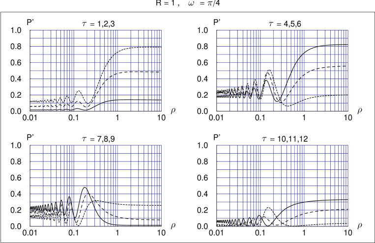
Figure 6: Same as Fig. 5 but for the time-reversed process, with probability $P^{\prime}\equiv P(\nu_{e}\rightarrow\nu_{\mu})$. If CPT invariance holds, $P^{\prime}$ also corresponds to $P(\overline{\nu}_{\mu}\rightarrow\overline{\nu}_{e})$.

In the previous paragraph and corresponding Appendix, the stealth-like behavior of the $R=1$, $\omega=\pi/4$ model has been emphasized, but this holds only for the $\nu_{\mu}\rightarrow\nu_{e}$ channel relevant to superbeam experiments with an initial $\nu_{\mu}$ beam from pion and kaon decays. In other channels, the situation may be different. The probability $P_{e\mu}$ of the $\nu_{e}\rightarrow\nu_{\mu}$ channel, for example, is given in Fig. 6. The very different probabilities of Figs. 5 and 6, for $\rho\gtrsim 0.2$ and generic values of $\tau$, signal time-reversal (T) noninvariance.

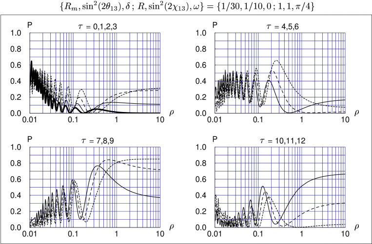
Figure 7: Same as Fig. 5 but now for mass-sector parameters $R_{m}\equiv\Delta m^{2}_{21}/\Delta m^{2}_{32}=1/30$, $\sin^{2}(2\theta_{13})=1/10$, and $\delta=0$. The heavy solid curve in the upper left panel has $\tau=0$, corresponding to pure mass-difference neutrino oscillations.

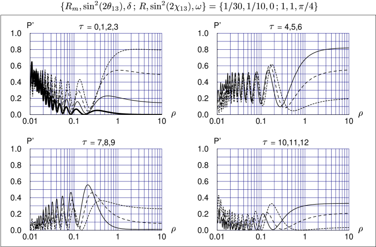
Figure 8: Same as Fig. 7 but for the time-reversed process, with probability $P^{\prime}\equiv P(\nu_{e}\rightarrow\nu_{\mu})$. If CPT invariance holds, $P^{\prime}$ also corresponds to $P(\overline{\nu}_{\mu}\rightarrow\overline{\nu}_{e})$.

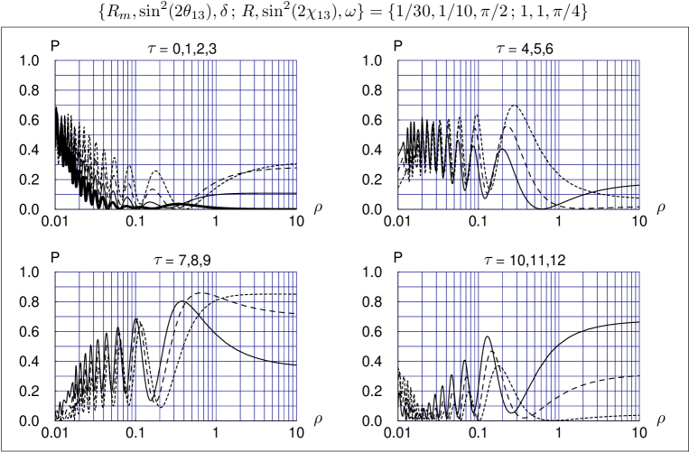
Figure 9: Same as Fig. 7 but now for $\delta=\pi/2$.

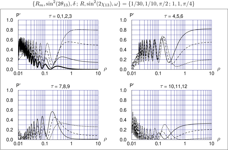
Figure 10: Same as Fig. 9 but for the time-reversed process, with probability $P^{\prime}\equiv P(\nu_{e}\rightarrow\nu_{\mu})$. If CPT invariance holds, $P^{\prime}$ also corresponds to $P(\overline{\nu}_{\mu}\rightarrow\overline{\nu}_{e})$.

For comparison, we give in Figs. 7–10 the numerical results from a “realistic” mass sector: $R_{m}\equiv\Delta m^{2}_{21}/\Delta m^{2}_{32}\approx 0.033$, $\sin^{2}(2\theta_{13})=0.1$ [close to the experimental bound from Chooz], and two possible values of the complex phase, $\delta=0$ or $\delta=\pi/2\,$. Figures 9 and 10, in particular, show that the maximum T–violation discriminant $\Delta_{T}\equiv P_{e\mu}-P_{\mu e}$ from pure mass-difference neutrino oscillations ($\tau=0$) is of the order of several percent, much less than the potential Fermi-point-splitting result (several tens of percent) at the high-energy end of the neutrino spectrum.

The strong high-energy T violation (and possibly CP violation Klinkhamer-IJMPA ) from Figs. 5–10 traces back to the large complex phase $\omega$ of the model considered, together with the large mixing angles $\chi_{ij}$ and splitting ratio $R$ in the Fermi-point-splitting sector. In other words, the breaking of time-reversal invariance would primarily take place outside the mass sector. A neutrino factory (see Ref. Bueno-etal2001 and the Appendix) would be the ideal machine, in principle, to establish such strong T violation in high-energy neutrino oscillations.

Appendix A Case study

In this appendix, we give a concrete example of the complicated phenomenology of stealth–type models. Take, then, the generalized model (1)–(16) with parameters $\omega=\pi/4$ and $\Delta b_{0}^{(31)}=2\,\Delta b_{0}^{(21)}=3.5\times 10^{-12}\;\mathrm{eV}$ and consider the combined performance of four accelerator-based neutrino-oscillation experiments T'Jampens-NuFact04 ; Harris-NuFact04 : the current K2K experiment (baseline $L=250\;\mathrm{km}$ and peak energy $\overline{E}_{\nu}\approx 1.0\;\mathrm{GeV}$), the running MINOS experiment ($L=735\;\mathrm{km}$ and $\overline{E}_{\nu}\approx 3.75\;\mathrm{GeV}$, in the LE mode), the planned T2K experiment ($L=295\;\mathrm{km}$ and $\overline{E}_{\nu}\approx 0.7\;\mathrm{GeV}$, for an off-axis beam at $2$ degrees), and the proposed NO$\nu$A experiment ($L=810\;\mathrm{km}$ and $\overline{E}_{\nu}\approx 2\;\mathrm{GeV}$, at $14\;\mathrm{mrad}$ offset in the ME mode). At the end of this appendix, we also comment briefly on the capabilities of a possible neutrino factory.

First, calculate the model predictions for the two current experiments. For K2K, the neutrino-oscillation parameters would be $\tau\approx 4.4$ and $\rho\approx 0.63$, so that a value for $P_{\mu e}\equiv P(\nu_{\mu}\rightarrow\nu_{e})$ of only $1\,\%$ would be expected (cf. solid curve in upper right panel of Fig. 5), which is consistent with the experimental result K2K-electron . [Note that the K2K appearance probability $P_{\mu e}$ would be approximately $15\,\%$ for the model with vanishing complex phase $\omega$, as indicated by the solid curve in the upper right panel of Fig. 4.] For the MINOS–LE experiment with $\tau\approx 13.0$ and $\rho\approx 0.81$, a relatively small probability $P_{\mu e}\approx 7\,\%$ would be expected, which would perhaps be hard to separate from the background. [Note that this $\tau$–value corresponding to the MINOS baseline is an order of magnitude above the largest one of Fig. 1.] Hence, the model predictions of the appearance probability $P_{\mu e}$, for the chosen parameters, would be consistent with rather low $\nu_{e}$ event rates from both of these current experiments. For completeness, the model would also give a survival probability $P_{\mu\mu}\equiv P(\nu_{\mu}\rightarrow\nu_{\mu})$ of some $49\,\%$ for K2K and $87\,\%$ for MINOS–LE.

Next, turn to the model predictions for the two future experiments considered. For T2K with $\tau\approx 5.2$ and $\rho\approx 0.38$, a substantial $P_{\mu e}$ of some $25\,\%$ would be expected (cf. long-dashed curve in upper right panel of Fig. 5). Similarly, for NO$\nu$A with $\tau\approx 14.4$ and $\rho\approx 0.39$, $P_{\mu e}$ would be approximately $27\,\%$. Hence, the model predictions of the appearance probability $P_{\mu e}$ would imply a clear signal in these future experiments, at least for the chosen parameters. Again, for completeness, the model survival probability $P_{\mu\mu}$ would be approximately $71\,\%$ for T2K and $20\,\%$ for NO$\nu$A.

Ultimately, the lowest values of $|\Delta b_{0}^{(31)}|$ could be probed by a neutrino factory with broad energy spectrum $E_{\nu}\approx 10-50\;\mathrm{GeV}$ and several detectors at baselines $L$ up to $12800\;\mathrm{km}$; see, e.g., Refs. Bueno-etal2001 ; CERNreportNuFact ; NuFact04 . For a quick estimate, one can simply compare the expected experimental capabilities with the approximate vacuum probability (18), for $\rho=\mathrm{O}(1)$ and $\tau\ll 1$ as defined by (17). In the best of all worlds, a $P_{\mu e}$ sensitivity of $0.01\,\%$ at $L=7350\;\mathrm{km}$ and $E_{\nu}\approx 46\;\mathrm{GeV}$, for example, would correspond to $|\Delta b_{0}^{(31)}|$ of the order of $10^{-15}\;\mathrm{eV}$. However, for a definite analysis at these large distances, matter effects endnote-matter would need to be folded in.

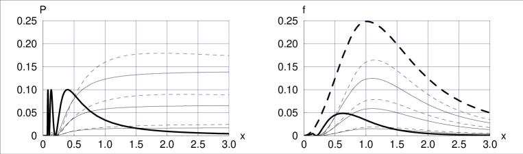
Figure 1: Left: Fixed-distance vacuum probabilities $P_{\mu e}\equiv P(\nu_{\mu}\rightarrow\nu_{e})$ at $l\equiv L/\overline{L}\equiv L\,|\Delta m^{2}_{31}|/(2\pi\overline{E}_{\nu})=735/1860$ vs. dimensionless energy $x\equiv E_{\nu}/\overline{E}_{\nu}$ for the “stealth” model of Ref. KlinkhamerTheta13 with both mass differences and timelike Fermi-point splittings, here defined by Eqs. (1)–(16). The broken curves are given by the analytic expression (4.4) of Ref. KlinkhamerTheta13 with parameters $\overline{\Theta}_{13}\equiv\overline{E}_{\nu}\,|\Delta b_{0}^{(31)}|/|\Delta m^{2}_{31}|=0.15,\,0.30,\,0.45$, which correspond to Fermi-point splittings $|\Delta b_{0}^{(13)}|\approx(1.0,\,2.0,\,3.0)\times 10^{-13}\;\mathrm{eV}$ for $\overline{E}_{\nu}=3.75\;\mathrm{GeV}$ and $\Delta m^{2}_{31}=2.5\times 10^{-3}\;\mathrm{eV}^{2}$. The same analytic expression is given here by Eq.  (18) with parameters $\tau\approx(0.37,\,0.74,\,1.12)$. These broken curves are only approximate and the corresponding thin solid curves give the full numerical results. The heavy solid curve gives, for comparison, the standard mass-difference probability $P_{\mu e}^{\text{MD}}$ for $\Delta m^{2}_{21}=0$, $\sin^{2}\theta_{32}=1/2$, $\sin^{2}(2\,\theta_{13})=0.2$, and $l=735/1860$. Right: Electron–type neutrino energy spectra $f_{e}(x)$ at $l=735/1860$ from an initial muon–type spectrum (4.8) of Ref. KlinkhamerTheta13 at $l=0$ and vacuum probabilities $P(\nu_{\mu}\rightarrow\nu_{e})$ of the left panel. The initial $\nu_{\mu}$ spectrum multiplied by a constant factor $0.25$ is shown as the heavy long-dashed curve. The resulting $\nu_{e}$ spectra from the “stealth” model are shown as the thin solid curves [approximate values as thin broken curves]. The heavy solid curve gives, for comparison, the $\nu_{e}$ spectrum from the standard mass-difference probability $P_{\mu e}^{\text{MD}}$ of the left panel.

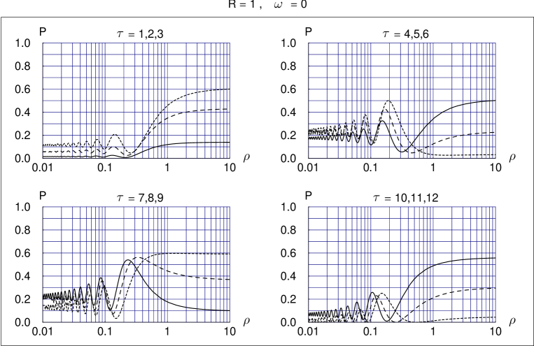
Figure 4: Same as Fig. 3 but for the generalized model with splitting ratio $R\equiv|\Delta b_{0}^{(21)}/\Delta b_{0}^{(32)}|=1$, the complex phase $\omega$ still vanishing.

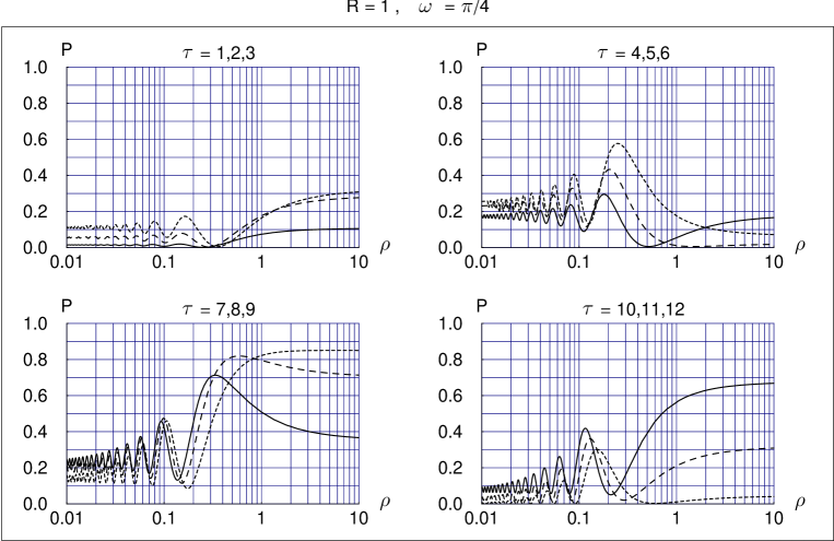
Figure 5: Same as Fig. 4 but now for the generalized model with complex phase $\omega=\pi/4$.

References

• (1) F.R. Klinkhamer, “Possible energy dependence of $\Theta_{13}$ in neutrino oscillations,” Phys. Rev. D 71, 113008 (2005) [hep-ph/0504274].
• (2) Matter effects (coherent forward scattering) from the Earth’s mantle become important for standard mass-difference neutrino oscillations at energies $E_{\nu}$ of order $10\;\mathrm{GeV}$ and travel distances $L$ of order $2500\;\mathrm{km}$. For further details and references, see, e.g., Ref. Bueno-etal2001 and Ref. CERNreportNuFact , Chapter 3 [hep-ph/0210192].
• (3) A. Bueno, M. Campanelli, S. Navas-Concha, and A. Rubbia, “On the energy and baseline optimization to study effects related to the $\delta$–phase (CP–/T–violation) in neutrino oscillations at a neutrino factory,” Nucl. Phys. B 631, 239 (2002) [hep-ph/0112297].
• (4) A. Blondel et al., ECFA/CERN studies of a European neutrino factory complex, report CERN-2004-002, April 2004.
• (5) In the combined limit $\rho\to\infty$ and $\tau\to 0$, the factor $\widehat{\Lambda}_{\mu e}$ behaves as $\mathrm{O}(1/\rho)+\mathrm{O}(\tau)$, i.e., proportional to $L\,$. Note also that, in first approximation, $\widehat{\Lambda}_{\mu e}$ is assumed to contain no further factors which only depend on the product $\rho\tau$. In addition, it is necessary to consider all channels in order to make, as far as possible, a useful distinction between the quantities $\widehat{\Theta}_{32}$ and $\widehat{\Theta}_{13}$ in Eq. (19a).
• (6) F.R. Klinkhamer, Neutrino oscillations from the splitting of Fermi points, JETP Lett. 79, 451 (2004) [hep-ph/0403285].
• (7) F.R. Klinkhamer, Lorentz-noninvariant neutrino oscillations: Model and predictions, Int. J. Mod. Phys. A 21, 161 (2006) [hep-ph/0407200].
• (8) Note that the notation for the neutrino dispersion relation in Refs. Klinkhamer-JETPL ; Klinkhamer-IJMPA differs from the one used here and in Ref. KlinkhamerTheta13 . For neutrino oscillations in the pure Fermi-point-splitting model Klinkhamer-JETPL ; Klinkhamer-IJMPA , the different sign of $b_{0}^{(f)}$ can be compensated by a sign change of the complex phase $\epsilon$. For example, setting $\epsilon=-\omega$ in the exact model probablity $P_{\mu e}$ from Eq. (11e) of Ref. Klinkhamer-IJMPA reproduces the numerical $\rho\to\infty$ results for $R=1$, $\chi_{21}=\chi_{32}=\pi/4$, $\chi_{13}=\arctan\sqrt{1/2}\approx\pi/5$, and $\omega=0$ or $\pi/4$ (these numerical results closely resemble those for $\chi_{13}=\pi/4$ presented in Figs. 4 and 5 here).
• (9) Degenerate perturbation theory for $\rho\to 0$ and fixed $\tau$ (arbitrary $R$ and $\omega$) gives $P_{\mu e}\sim(4R^{2}/S)\,\sin^{2}\,[\sqrt{S}\,\tau/(8+8R)]$ with $S\equiv 4+4R+9R^{2}$. For $R=1$, in particular, the $\rho\to 0$ probablity is given by $P_{\mu e}\sim(4/17)\,\sin^{2}\,[\sqrt{17}\,\tau/16]$. If, however, the mass-hierarchy parameter $R_{m}\equiv\Delta m^{2}_{21}/\Delta m^{2}_{32}$ is changed from zero to $1/30$, the $\rho\lesssim 0.1$ behavior changes significantly, as will become clear later on.
• (10) S. T’Jampens, Current and near future long-baseline neutrino experiments, in Ref. NuFact04 , p. 24.
• (11) D.A. Harris, Superbeam Experiments, in Ref. NuFact04 , p. 34.
• (12) Proceedings 6th International Workshop on Neutrino Factories and Superbeams (NuFact04), edited by M. Aoki, Y. Iwashita, and M. Kuze, Nucl. Phys. B (Proc. Suppl.) 149 (2005), pp. 1–411.
• (13) M.H. Ahn et al. [K2K Collaboration], Search for electron neutrino appearance in a 250-km long-baseline experiment, Phys. Rev. Lett. 93, 051801 (2004), hep-ex/0402017; K. Kaneyuki, K2K far detector analysis, in Ref. NuFact04 , p. 119.
Refer to caption