Ideal Fermion Delocalization
in Five Dimensional Gauge Theories

Abstract:

We discuss ideal delocalization of fermions in a bulk $SU(2)\times SU(2)\times U(1)$ Higgsless model with a flat or warped extra dimension. So as to make an extra dimensional interpretation possible, both the weak and hypercharge properties of the fermions are delocalized, with the $U(1)_{Y}$ current of left-handed fermions being correlated with the $SU(2)_{W}$ current. We find that (to subleading order) ideal fermion delocalization yields vanishing precision electroweak corrections in this continuum model, as found in corresponding theory space models based on deconstruction. In addition to explicit calculations, we present an intuitive argument for our results based on Georgi’s spring analogy. We also discuss the conditions under which the essential features of an $SU(2)\times SU(2)\times U(1)$ bulk gauge theory can be captured by a simpler $SU(2)\times SU(2)$ model.

1 Introduction

Higgsless models [1] have gained popularity because of their ability to provide an alternative mechanism of electroweak symmetry breaking that forgoes a scalar Higgs boson [2]. Much has been written about models [3, 4] based on a five-dimensional $SU(2)\times SU(2)\times U(1)$ gauge theory in a slice of Anti-deSitter space, in which electroweak symmetry breaking is encoded in the boundary conditions of the gauge fields. The spectrum includes states identified with the photon, $W$, and $Z$, and also an infinite tower of additional massive vector bosons (the higher Kaluza-Klein or $KK$ excitations), whose exchange is responsible for unitarizing longitudinal $W$ and $Z$ boson scattering [5, 6, 7, 8].

The properties of Higgsless models may be studied [9, 10, 11, 12, 13, 14, 15, 16] using deconstruction [17, 18] which leads one to compute the electroweak parameters $\alpha S$ and $\alpha T$ [19, 20, 21] in a related linear moose model [22]. We have shown [16] how to compute all four of the leading zero-momentum electroweak parameters defined by Barbieri et. al. [23] in a very general class of linear moose models. We have demonstrated that a Higgsless model with localized fermions cannot simultaneously satisfy (1) unitarity bounds, (2) provide acceptably small precision electroweak corrections, and (3) have no light vector bosons other than the photon, $W$, and $Z$. We also found that localizing the hypercharge properties of the fermions at a single $U(1)$ site adjacent to the chain of $SU(2)$ groups on the linear moose caused $\Delta\rho$ ($Y$ in the language of Barbieri et al. [23]) to vanish.

Following proposals [24, 25, 26] that delocalizing fermions within the extra dimension can reduce electroweak corrections, we showed [29] in an arbitrary Higgsless model that choosing the probability distribution of the delocalized fermions to be related to the wavefunction of the $W$ boson makes the other three ($\hat{S}$, $\hat{T}$, $W$) leading zero-momentum precision electroweak parameters defined by Barbieri, et. al. [23] vanish at tree-level. We denote such fermions as “ideally delocalized”.

In this paper, we provide a continuum realization of ideal delocalization that preserves the characteristic of vanishing precision electroweak corrections up to subleading order. The challenge is as follows. We have found that deconstructed models with $\Delta\rho=0$ have the hypercharge current of fermions localized at one site while models with small $\hat{S}$, $\hat{T}$ and $W$ have the weak current of fermions ideally delocalized over many sites. This situation is perfectly consistent in the context of a theory-space moose model, but is difficult to interpret as a model with an extra dimension. After all, left-handed quarks and leptons carry both $SU(2)$ and $U(1)$ charges, yet should have a single profile along the extra dimension.

We show here that arranging for the delocalization of the left-handed $U(1)$ fermion current to be correlated with the ideal delocalization of the fermions’ $SU(2)$ properties provides a resolution in the context of a bulk $SU(2)\times SU(2)\times U(1)$ model. The moose diagram corresponding to this continuum model is shown in Fig. 1. Two species of bulk fermions are introduced. Fermion $A$ feels the $SU(2)$ gauge field of the $A$-branch weak groups, while fermion $B$ couples to the $B$-branch fields; both couple with the same bulk $U(1)$ gauge field. By calculating the profiles of the gauge bosons and fermions, and their couplings to one another, we will demonstrate that ideal fermion delocalization, as realized here in the continuum, still ensures the vanishing of the leading zero-momentum electroweak precision observables – including $\Delta\rho$. Moreover, we will find that the essential features of the theory-space model can be captured by an even simpler $SU(2)\times SU(2)$ continuum model, which can then be used to study other aspects of the phenomenology of Higgsless models [30].

Section 2 uses Georgi’s spring analogy [15] to provide an intuitive understanding of the correspondence between the $SU(2)^{2}\times U(1)$ model and the $SU(2)^{2}$ model. Sections 3 and 4 provide detailed analyses of ideal delocalization in bulk $SU(2)\times SU(2)\times U(1)$ models in flat and warped space, respectively. The calculation of electroweak observables and is discussed in section 5. In section 6 we consider the effect of a TeV brane $U(1)$ kinetic energy term and show that, unlike the case of a Planck brane term, there is no correspondence to an $SU(2)^{2}$ model and there are nontrivial electroweak corrections. Section 7 presents our conclusions.

2 Mass-Spring Analogy

In this paper, we study ideal fermion delocalization in the context of a five-dimensional $SU(2)_{A}\otimes SU(2)_{B}\otimes U(1)$ gauge theory, considering both the case in which the fifth dimension is flat and the case in which it is warped. The coupling of both $SU(2)$ groups is denoted $g_{5W}$ while that of the hypercharge group is written $g_{5Y}$. We also introduce brane kinetic terms of strength $g_{0}$ and $g_{Y}$ for $SU(2)_{A}$ and $U(1)$, respectively. The corresponding moose model is shown in Fig. 1.

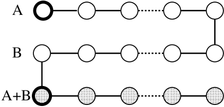
Figure 1: The moose description of the extra dimension model discussed in this paper. The unshaded and shaded circles represent $SU(2)$ and $U(1)$ gauge fields; brane kinetic terms are located at the thick circles. Two species of bulk fermions are introduced: fermion $A$ feels the gauge fields of the $A$-branch of $SU(2)$, while fermion $B$ couples to the $B$-branch fields. Both fermions couple to the same bulk $U(1)$ gauge field. The delocalization of left-handed $U(1)_{Y}$ current is therefore correlated with the $SU(2)_{W}$ delocalization.

Explicit analyses presented in sections 3-5 will demonstrate that all four leading precision electroweak parameters ($\alpha S$, $\alpha T$, $\Delta\rho$, and $\alpha\delta$ [14]) vanish to order $M^{2}_{W}/M^{2}_{W1}$. It will also be shown that the $\gamma$, $W$, and $Z$ couplings and wavefunctions in this model are equivalent to those in an effective $SU(2)\times SU(2)$ model with a $U(1)$ brane kinetic energy term of appropriate strength. Before diving into the detailed calculation, we would like to provide an intuitive basis for understanding our results, using Georgi’s spring analogy [15].

Figure 2: Linear moose diagram equivalent to Fig.1. The distribution of a left-handed fermion’s $U(1)_{Y}$ current is correlated with the $SU(2)_{W}$ current.

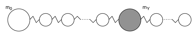
Figure 3: Spring system corresponding to the neutral gauge-boson sector of $SU(2)^{2}\times U(1)$ models. $m_{0}=1/g^{2}_{0}$ and $m_{Y}=1/g^{2}_{Y}$ are larger than all of the other masses in the chain.

The moose for the $SU(2)^{2}\times U(1)$ model may be redrawn as shown in Fig. 2. It is now straightforward to use Georgi’s spring analogy to see that the spring system whose eigenmodes correspond to the neutral gauge-boson mass eigenstates has the form shown in Fig. 3. Here we associate each gauge group with a mass $m_{i}$, each link with a massless spring with Hooke’s law constant $k_{i}$, and the spring displacements ($x_{i}$) with the amplitudes of the corresponding eigenvectors of the gauge-boson mass matrix using [15] the correspondence

$$x_{i}\leftrightarrow g_{i}A^{\mu}_{i}~{},\quad\quad\quad k_{i}\leftrightarrow\frac{f^{2}_{i}}{4}~{},\quad\quad\quad m_{i}\leftrightarrow\frac{1}{g^{2}_{i}}~{}.$$ (1)

Under this correspondence, the mass-squareds of the gauge-boson eigenstates correspond to the squared frequencies of the spring system, and the eigenmodes of the spring system correspond to the amplitudes of the corresponding gauge-boson eigenstates [15].

Let us first consider the case of a flat extra dimension. In order to obtain light $W$ and $Z$ bosons, we work in the limits

$$\frac{1}{g^{2}_{Y}}\gg\frac{\pi R}{g^{2}_{5Y}}~{}\quad\quad\frac{1}{g^{2}_{0}}\gg\frac{2\pi R}{g^{2}_{5W}}$$ (2)

and therefore the corresponding masses $m_{0}=1/g^{2}_{0}$ and $m_{Y}=1/g^{2}_{Y}$ in Fig. 3 are drawn as large. These conditions are required in order that the $W$ and $Z$ be much lighter than the $KK$ resonances in these models [15, 16].

Consider the neutral gauge boson sector. Using our physical intuition, it is easy to see which spring system eigenmodes correspond to the photon and the $Z$-boson. The photon, which is massless, corresponds to the uniform translation of the spring system – i.e. to a “flat” gauge-boson profile (see eqn. (1)) in which $g_{i}A_{i}$ is constant. Since there is no restoring force for this motion, this corresponds to a zero mode and therefore a massless photon.

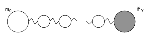
Figure 4: Spring system corresponding to the neutral gauge-boson sector of an $SU(2)^{2}$ model with $\tilde{m_{Y}}$ an effective mass as in eqn. (3).

If $m_{0}$ and $m_{Y}$ are much larger than all of the other masses, the next lightest (low-frequency) mode corresponds to a “breathing mode” in which masses $m_{0}$ and $m_{Y}$ oscillate slowly opposite to one another. In this mode, the masses in the spring system between $m_{0}$ and $m_{Y}$ oscillate adiabatically, but the masses in the chain to the right of $m_{Y}$ oscillate uniformly with no relative motion. That is, the masses in the chain to the right of $m_{Y}$ have, again, a flat profile. To leading order, the only effect of the masses to the right of $m_{Y}$ is to change the effective mass of $m_{Y}$ to

$$\tilde{m}_{Y}=m_{Y}+\sum_{U(1)\,chain}m_{\ell}~{},$$ (3)

where the sum extends over all of the masses to the right of $m_{Y}$ – all masses in the “$U(1)$ chain.” Corrections to this picture due to oscillatory motion within the $U(1)$ chain, will be suppressed by $m^{2}_{\ell}/\tilde{m}^{2}_{Y}$. To this order, therefore, the properties of the oscillatory modes corresponding to both the photon and $Z$ are equivalent to those calculated in the spring system shown in Fig. 4. But this spring system corresponds to the neutral gauge-boson sector of an $SU(2)^{2}$ linear moose in which, as suggested by eqn. (3), the strength $g_{Y{\rm eff}}$ of the hypercharge brane kinetic energy term is taken to satisfy the relation

$$\frac{1}{g^{2}_{Y{\rm eff}}}=\frac{1}{g^{2}_{Y}}+\frac{\pi R}{g^{2}_{5Y}}~{}.$$ (4)

The properties of the $W$ boson and the charged KK resonances $W_{(n\geq 1)}$ are independent of the $U(1)$ portion of the moose. These charged eigenmodes are therefore identical in the $SU(2)^{2}\otimes U(1)$ and $SU(2)^{2}$ linear mooses discussed here. In addition, we note that the contribution of the $SU(2)^{2}$ groups to the properties of the neutral gauge bosons is the same in both models.

Finally, we may consider the corresponding situation in a Higgsless model in warped space. At first sight, the situation here appears to be different: the common deconstruction of this model has a single gauge coupling and geometrically varying $f$-constants [31, 32]. However, one may choose an alternative ‘f-flat’ deconstruction [29, 33] in which the couplings vary but the $f$-constants do not. In this alternate deconstruction, the analysis given above for a flat space model applies directly.

In sections 3 and 4 of this paper, we will see that the physical intuition just presented is born out by explicit calculations of the properties of the photon, $W$, and $Z$ bosons in a bulk $SU(2)^{2}\times U(1)$ Higgsless model of electroweak symmetry breaking. Moreover, because the precision electroweak corrections $\alpha S$, $\alpha T$, $\Delta\rho$ and $\alpha\delta$ measure the degree to which the $W$ and $Z$ bosons of a given model differ from those of the Standard Model, we expect that the values of these precision observables will be the same, to leading order, for the $SU(2)^{2}\otimes U(1)$ and $SU(2)^{2}$ models discussed here. Again, we will find, in section 5, that this is supported by explicit calculations. Note that this agreement occurs despite the fact that the profiles of the individual higher neutral KK resonances will be different in the two models.

3 Explicit Calculations in Flat Space

We consider a five-dimensional $SU(2)_{A}\otimes SU(2)_{B}\otimes U(1)$ gauge theory in flat space, in which the fifth dimension (denoted by the coordinate $y$) is compactified on an interval of length $\pi R$. In order to make $M_{W}$ and $M_{Z}$ sufficiently lighter than the other KK masses, we also introduce kinetic terms for $SU(2)_{A}$ and $U(1)$ on the $y=0$ brane. The continuum 5D action corresponding to Fig. 1 is then given by

$$S = \int_{0}^{\pi R}dy\int d^{4}x\left\{-\frac{1}{4g_{0}^{2}}\delta(y-0^{+})W^{a}_{A\mu\nu}W^{a}_{A\rho\lambda}\eta^{\mu\rho}\eta^{\nu\lambda}-\frac{1}{4g_{Y}^{2}}\delta(y-0^{+})B_{\mu\nu}B_{\rho\lambda}\eta^{\mu\rho}\eta^{\nu\lambda}\right\}$$ (5)

$$+\int_{0}^{\pi R}dy\int d^{4}x\dfrac{1}{g_{5WA}^{2}}\left\{-\frac{1}{4}W^{a}_{A\mu\nu}W^{a}_{A\rho\lambda}\eta^{\mu\rho}\eta^{\nu\lambda}+\frac{1}{2}W^{a}_{A\mu y}W^{a}_{A\nu y}\eta^{\mu\nu}\right\}$$

$$+\int_{0}^{\pi R}dy\int d^{4}x\dfrac{1}{g_{5WB}^{2}}\left\{-\frac{1}{4}W^{a}_{B\mu\nu}W^{a}_{B\rho\lambda}\eta^{\mu\rho}\eta^{\nu\lambda}+\frac{1}{2}W^{a}_{B\mu y}W^{a}_{B\nu y}\eta^{\mu\nu}\right\}$$

$$+\int_{0}^{\pi R}dy\int d^{4}x\dfrac{1}{g_{5Y}^{2}}\left\{-\frac{1}{4}B_{\mu\nu}B_{\rho\lambda}\eta^{\mu\rho}\eta^{\nu\lambda}+\frac{1}{2}B_{\mu y}B_{\nu y}\eta^{\mu\nu}\right\},$$

with $W^{a}_{A\mu}$ ($W^{a}_{B\mu}$) being the $SU(2)$ gauge fields in the $A$-($B-$)branches and $B_{\mu}$ being the $U(1)$ gauge field. These gauge fields satisfy boundary conditions,

$$\partial_{y}W^{a}_{A\mu}=0,\qquad W^{1,2}_{B\mu}=0,\qquad W^{3}_{B\mu}=B_{\mu},\qquad\dfrac{1}{g_{5WB}^{2}}\partial_{y}W^{3}_{B\mu}+\dfrac{1}{g_{5Y}^{2}}\partial_{y}B_{\mu}=0,$$ (6)

at $y=0$, which break the original gauge group to $SU(2)_{W}\times U(1)_{Y}$, and boundary conditions

$$W^{a}_{A\mu}=W^{a}_{B\mu},\qquad\dfrac{1}{g_{5WA}^{2}}\partial_{y}W^{a}_{A\mu}+\dfrac{1}{g_{5WB}^{2}}\partial_{y}W^{a}_{B\mu}=0,\qquad\partial_{y}B_{\mu}=0,$$ (7)

at $y=\pi R$, which break $SU(2)_{A}\times SU(2)_{B}$ to its diagonal subgroup. For simplicity, in the following analyses, we assume the bulk $SU(2)$ gauge couplings in the $A$ and $B$ branches are identical: $g_{5W}^{2}=g_{5WA}^{2}=g_{5WB}^{2}$.

We can unfold the original moose of Fig. 1, to obtain an equivalent linear moose model as shown in Fig. 2. The corresponding continuum action is

$$S = \int_{0}^{3\pi R}\!\!dy\int d^{4}x\left\{-\frac{1}{4g_{0}^{2}}\delta(y-0^{+})W^{a}_{\mu\nu}W^{a}_{\rho\lambda}\eta^{\mu\rho}\eta^{\nu\lambda}-\frac{1}{4g_{Y}^{2}}\delta(y-2\pi R-0^{+})B_{\mu\nu}B_{\rho\lambda}\eta^{\mu\rho}\eta^{\nu\lambda}\right\}$$ (8)

$$+\int_{0}^{2\pi R}dy\int d^{4}x\dfrac{1}{g_{5W}^{2}}\left\{-\frac{1}{4}W^{a}_{\mu\nu}W^{a}_{\rho\lambda}\eta^{\mu\rho}\eta^{\nu\lambda}+\frac{1}{2}W^{a}_{\mu y}W^{a}_{\nu y}\eta^{\mu\nu}\right\}$$

$$+\int_{2\pi R}^{3\pi R}dy\int d^{4}x\dfrac{1}{g_{5Y}^{2}}\left\{-\frac{1}{4}B_{\mu\nu}B_{\rho\lambda}\eta^{\mu\rho}\eta^{\nu\lambda}+\frac{1}{2}B_{\mu y}B_{\nu y}\eta^{\mu\nu}\right\},$$

with boundary conditions

$${\rm at\ }y = 0:\ \ \ \ \qquad\qquad\partial_{y}W^{a}_{\mu}=0$$ (9)

$${\rm at\ }y = 2\pi R:\qquad\qquad W^{1,2}_{\mu}=0,\qquad\dfrac{1}{g_{5W}^{2}}\partial_{y}W^{3}_{\mu}=\dfrac{1}{g_{5Y}^{2}}\partial_{y}B_{\mu}$$ (10)

$${\rm at\ }y = 3\pi R:\qquad\qquad\partial_{y}B_{\mu}=0.$$ (11)

For the Fig. 2 linear moose, the weak $SU(2)$ current distribution of a fermion, $|\psi(y)|_{W}^{2}$, is defined on $y\in[0,2\pi R)$, while the left-handed $U(1)$ hypercharge distribution, $|\psi(y)|_{Y}^{2}$, takes its value on $y\in[2\pi R,3\pi R)$. These current distributions are correlated, as a consequence of the original folded structure (Fig. 1):

$$|\psi(y+2\pi R)|_{Y}^{2}=|\psi(y)|_{W}^{2}+|\psi(2\pi R-y)|_{W}^{2},\qquad\mbox{for $\pi R\geq y\geq 0$}.$$ (12)

This observation is what makes it possible to generalize our results [29, 30] for theory-space models with ideal fermion delocalization to five-dimensional gauge theories.

3.1 Mode equations and modified BCs

The 5D fields $W^{a}_{\mu}(x,y)$ and $B_{\mu}(x,y)$ can be decomposed into KK-modes,

$$W_{\mu}^{1,2}(x,y) = \sum_{n}W_{\mu}^{(n)1,2}(x)\chi_{W(n)}(y),$$ (13)

$$W_{\mu}^{3}(x,y) = \gamma_{\mu}(x)\chi_{\gamma}(y)+\sum_{n}Z_{\mu}^{(n)}\chi_{Z(n)}(y),\qquad\mbox{for $y<2\pi R$},$$ (14)

$$B_{\mu}(x,y) = \gamma_{\mu}(x)\chi_{\gamma}(y)+\sum_{n}Z_{\mu}^{(n)}\chi_{Z(n)}(y),\qquad\mbox{for $y>2\pi R$}.$$ (15)

Here $\gamma_{\mu}(x)$ is the photon, and $W_{\mu}^{(n)\,1,2}(x)$ and $Z_{\mu}^{(n)}(x)$ are the $KK$ towers of the massive $W$ and $Z$ bosons, the lowest of which correspond to the observed $W$ and $Z$ bosons. Since the lightest massive $KK$-modes are identified as the observed $W$ and $Z$ bosons, we write

$$M_{W}^{2} \equiv M_{W_{(0)}}^{2},\ \ \ \ \ M_{Z}^{2}\equiv M_{Z_{(0)}}^{2}~{},$$ (16)

$$\chi_{W} \equiv \chi_{W_{(0)}}~{},\ \ \ \ \ \chi_{Z}\equiv\chi_{Z_{(0)}}~{}.$$ (17)

These mode functions obey differential equations derived from the 5D Lagrangian eqn. (8):

$$0=\partial_{y}^{2}\chi_{W}(y)+M_{W}^{2}\chi_{W}(y),$$ (18)

$$0=\partial_{y}^{2}\chi_{Z}(y)+M_{Z}^{2}\chi_{Z}(y),$$ (19)

$$0=\partial_{y}^{2}\chi_{\gamma}(y).$$ (20)

which hold for $0^{+}<y<2\pi R$ and $2\pi R+0^{+}<y<3\pi R$. The presence of brane kinetic terms is reflected in modifications of the boundary conditions. We find

$$0=\left.\partial_{y}\chi_{W}(y)\right|_{y=0^{+}}+\dfrac{g_{5W}^{2}}{g_{0}^{2}}M_{W}^{2}\left.\chi_{W}(y)\right|_{y=0},\ \ \ \ \ 0=\left.\chi_{W}(y)\right|_{y=2\pi R},$$ (21)

for the $W$ mode function,

$$0=\left.\partial_{y}\chi_{Z}(y)\right|_{y=0^{+}}+\dfrac{g_{5W}^{2}}{g_{0}^{2}}M_{Z}^{2}\left.\chi_{Z}(y)\right|_{y=0},\ \ \ \ \ \left.\chi_{Z}(y)\right|_{y=2\pi R-0^{+}}=\left.\chi_{Z}(y)\right|_{y=2\pi R+0^{+}},$$ (22)

$$\dfrac{1}{g_{5W}^{2}}\partial_{y}\left.\chi_{Z}(y)\right|_{y=2\pi R-0^{+}}\ \ =\ \ \dfrac{1}{g_{5Y}^{2}}\partial_{y}\left.\chi_{Z}(y)\right|_{y=2\pi R+0^{+}}+\dfrac{1}{g_{Y}^{2}}M_{Z}^{2}\left.\chi_{Z}(y)\right|_{y=2\pi R},$$ (23)

$$0=\left.\partial_{y}\chi_{Z}(y)\right|_{y=3\pi R},$$ (24)

for the $Z$ mode function, and

$$0=\left.\partial_{y}\chi_{\gamma}(y)\right|_{y=0}\ \ \ \ \ \ \left.\chi_{\gamma}(y)\right|_{y=2\pi R-0^{+}}=\left.\chi_{\gamma}(y)\right|_{y=2\pi R+0^{+}},\ \ \ \ \ \ 0=\left.\partial_{y}\chi_{\gamma}(y)\right|_{y=3\pi R}$$ (25)

$$\dfrac{1}{g_{5W}^{2}}\left.\partial_{y}\chi_{\gamma}(y)\right|_{y=2\pi R-0^{+}}=\dfrac{1}{g_{5Y}^{2}}\left.\partial_{y}\chi_{\gamma}(y)\right|_{y=2\pi R+0^{+}}.$$ (26)

for the photon.

In order to obtain canonically normalized 4D fields ($W$, $Z$, $\gamma$), these mode functions are normalized as

$$1=\int_{0}^{2\pi R}\!\!dy\left\{\dfrac{1}{g_{5W}^{2}}+\dfrac{\delta(y-0^{+})}{g_{0}^{2}}\right\}\left|\chi_{W}(y)\right|^{2},$$ (27)

$$1=\int_{0}^{3\pi R}\!\!dy\left\{\dfrac{\theta(2\pi R-y)}{g_{5W}^{2}}+\dfrac{\delta(y-0^{+})}{g_{0}^{2}}+\dfrac{\theta(y-2\pi R)}{g_{5Y}^{2}}+\dfrac{\delta(y-2\pi R)}{g_{Y}^{2}}\right\}\left|\chi_{Z}(y)\right|^{2},$$

(28)

$$1=\int_{0}^{3\pi R}\!\!dy\left\{\dfrac{\theta(2\pi R-y)}{g_{5W}^{2}}+\dfrac{\delta(y-0^{+})}{g_{0}^{2}}+\dfrac{\theta(y-2\pi R)}{g_{5Y}^{2}}+\dfrac{\delta(y-2\pi R)}{g_{Y}^{2}}\right\}\left|\chi_{\gamma}(y)\right|^{2}.$$

3.2 Gauge Boson and Fermion Profiles

We now derive explicit expressions for the profiles of the gauge bosons and ideally delocalized fermions in the fifth dimension. To help the reader obtain an intuitive feel for the shapes of the wavefunctions, they are sketched in Fig. 5.

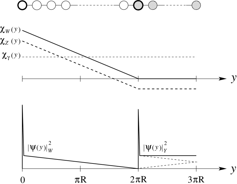
Figure 5: Sketch of the gauge boson mode functions and ideally delocalized fermion probability functions for the linear moose model. Note that, as seen from the text, $\chi_{Z}(0)\simeq c\,\chi_{W}(0)$ and $\chi_{\gamma}(0)\simeq s\,\chi_{W}(0)$ while $\chi_{Z}(y)$ is roughly parallel to $\chi_{W}(y)$. In addition, the fermion profile is flat in the hypercharge region $2\pi R<y<3\pi R$.

3.2.1 $W$ profile

The Dirichlet condition (21) at $y=2\pi R$ and the mode equation (18) determine the form of the $W$ mode function $\chi_{W}$,

$$\chi_{W}(y)\propto\sin\left[M_{W}(2\pi R-y)\right].$$ (30)

Because we are interested in situations where $W$ has a much lighter mass than the compactification scale $R^{-1}$,

$$M_{W}\ll\dfrac{1}{\pi R}.$$ (31)

we may expand eqn. (30) in terms of $M_{W}$,

$$\chi_{W}(y)=C_{W}\left(1-\dfrac{y}{2\pi R}\right)\left[1-\dfrac{4}{3!}\left(M_{W}\pi R\right)^{2}\left(1-\dfrac{y}{2\pi R}\right)^{2}+\cdots\right],$$ (32)

with $C_{W}$ being a normalization constant. The boundary condition (21) at $y=0$ then determines the size of the brane kinetic term, $g_{0}^{2}$, as a function of $M_{W}$:

$$g_{0}^{2}=2g_{5W}^{2}M_{W}^{2}\pi R\left[1+\frac{4}{3}(M_{W}\pi R)^{2}+\cdots\right],$$ (33)

which enables us to find the normalization constant $C_{W}$ from eqn. (27):

$$C_{W}^{2}=2g_{5W}^{2}M_{W}^{2}\pi R\left[1+\dfrac{4}{3}(M_{W}\pi R)^{2}+\cdots\right].$$ (34)

3.2.2 $Z$ profile

From the boundary condition (22) at $y=0$, we know the slope of $\chi_{Z}(y)$ at $y=0$. Higher derivative terms of $\chi_{Z}(y)$ at $y=0$ can also be calculated by using the mode equation (19). Taylor expansion near $y=0$ then gives

$$\chi_{Z}(y)=C_{Z}\left[1-\dfrac{g_{5W}^{2}}{g_{0}^{2}}M_{Z}^{2}y-\dfrac{1}{2}M_{Z}^{2}y^{2}+\dfrac{1}{3!}\dfrac{g_{5W}^{2}}{g_{0}^{2}}M_{Z}^{4}y^{3}+\cdots\right],$$ (35)

where $C_{Z}$ is a normalization constant. We note that this Taylor expansion can be viewed as an expansion in terms of $M_{Z}^{2}$, and also that $g_{0}^{2}$ is given as a function of $M^{2}_{W}$ in eqn. (33). Similar analysis can be done at $y=3\pi R$, where the slope of $\chi_{Z}$ vanishes thanks to the Neumann condition in eqn. (24). Taylor expansion around $y=3\pi R$ gives

$$\chi_{Z}(y)=\hat{C}_{Z}\left[1-\frac{1}{2}M_{Z}^{2}(3\pi R-y)^{2}+\cdots\right].$$ (36)

The continuity condition (22) at $y=2\pi R$ determines the ratio of constants $C_{Z}$ and $\hat{C}_{Z}$:

$$\hat{C}_{Z}=C_{Z}\left[1-2\dfrac{g_{5W}^{2}}{g_{0}^{2}}M_{Z}^{2}\pi R-\dfrac{3}{2}M_{Z}^{2}(\pi R)^{2}+\dfrac{1}{3}\dfrac{g_{5W}^{2}}{g_{0}^{2}}M_{Z}^{4}(\pi R)^{3}+\cdots\right]~{},$$ (37)

while eqn. (23) yields the size of the hypercharge brane kinetic term:

$$g_{Y}^{2}=2g_{5W}^{2}(M_{Z}^{2}-M_{W}^{2})\pi R\left[1+\frac{4}{3}(M_{Z}^{2}-2M_{W}^{2})(\pi R)^{2}+2\dfrac{g_{5W}^{2}}{g_{5Y}^{2}}(M_{Z}^{2}-M_{W}^{2})(\pi R)^{2}+\cdots\right].$$ (38)

From this result, we may derive an expression for $g_{Y\rm eff}$

$$\frac{1}{g_{Y{\rm eff}}^{2}}=\frac{1}{g_{Y}^{2}}+\frac{\pi R}{g_{5Y}^{2}}=\frac{1}{2g_{5W}^{2}(M_{Z}^{2}-M_{W}^{2})\pi R}\left(1-\frac{4}{3}(M_{Z}^{2}-2M_{W}^{2})(\pi R)^{2}+\cdots\right).$$ (39)

We are now ready to determine the normalization constant $C_{Z}$ from eqn. (28). Initially, it appeared that $C_{Z}$ might depend on the bulk $U(1)$ gauge coupling because of the non-trivial dependence on $g_{5Y}$ in the third term of eqn. (28). However, the fourth term in eqn. (28) also depends implicitly on $g_{5Y}$ through $g_{Y}^{2}$ (see eqn. (38)) and we find that the $g_{5Y}$ dependence in the two terms cancels at the order to which we are working. By examining the power counting in $M_{W,Z}^{2}$, we see that we can ignore the $y$ dependence of $\chi_{Z}$ for $y>2\pi R$ in eqn. (28) once eqn. (38) is applied. Performing the integral yields

$$\int_{0}^{3\pi R}\!\!dy\left\{\dfrac{\theta(y-2\pi R)}{g_{5Y}^{2}}+\dfrac{\delta(y-2\pi R)}{g_{Y}^{2}}\right\}\left|\chi_{Z}(y)\right|^{2}$$ (40)

$$\simeq \left(\dfrac{\pi R}{g_{5Y}^{2}}+\dfrac{1}{g_{Y}^{2}}\right)\left|\chi_{Z}(y=2\pi R)\right|^{2}$$

$$= \dfrac{1}{2g_{5W}^{2}(M_{Z}^{2}-M_{W}^{2})\pi R}\left(1-\frac{4}{3}(M_{Z}^{2}-2M_{W}^{2})(\pi R)^{2}+\cdots\right)\left|\chi_{Z}(y=2\pi R)\right|^{2}$$

which confirms the cancellation of all $g_{5Y}^{2}$ dependence at this order. After a straightforward calculation, we obtain the normalization constant $C_{Z}$

$$C_{Z}^{2}=2g_{5W}^{2}\dfrac{M_{W}^{4}}{M_{Z}^{2}}\pi R\left[1+\dfrac{4}{3}(M_{Z}^{2}-M_{W}^{2})(\pi R)^{2}+\cdots\right]~{}.$$ (41)

Note that in eqns. (37) and (41) neither hypercharge coupling ($g_{Y}$ or $g_{5Y}$) appears explicitly to this order – all dependence on these parameters has been absorbed into $M^{2}_{Z}$.

3.2.3 Photon profile

The photon mode function possesses a flat profile,

$$\chi_{\gamma}(y)=C_{\gamma},$$ (42)

with $C_{\gamma}$ being a normalization constant. The normalization condition eqn. (3.1) then reads

$$1=C_{\gamma}^{2}\left(\dfrac{2\pi R}{g_{5W}^{2}}+\dfrac{1}{g_{0}^{2}}+\dfrac{\pi R}{g_{5Y}^{2}}+\dfrac{1}{g_{Y}^{2}}\right).$$ (43)

Inserting eqn. (33) and eqn. (39) into this expression, we again observe the cancellation of the $g^{2}_{Y}$ and $g_{5Y}^{2}$ dependence between the third and the fourth terms. We find

$$C_{\gamma}^{2}=2g_{5W}^{2}M_{W}^{2}\pi R\left(1-\dfrac{M_{W}^{2}}{M_{Z}^{2}}\right)\left(1-\dfrac{4}{3}(M_{W}\pi R)^{2}+\cdots\right).$$ (44)

3.2.4 Ideally delocalized fermions

We now introduce the wavefunction assumed for the left-handed components of the ordinary fermions in this model. We focus here on ideally-delocalized fermions as defined in [29], which have been found, in theory-space Higgsless models, to yield small precision electroweak corrections. An ideally-delocalized fermion’s weak $SU(2)$ current distribution on $y\in[0,2\pi R)$ is derived from the $W$-boson profile:

$$|\psi(y)|^{2}_{W}\propto\left(\dfrac{1}{g_{0}^{2}}\delta(y-0^{+})+\dfrac{1}{g_{5W}^{2}}\right)\chi_{W}(y).$$ (45)

with the following normalization condition:

$$1=\int_{0}^{2\pi R}dy\,|\psi(y)|^{2}_{W}.$$ (46)

We thus obtain the ideally delocalized current distribution

$$|\psi(y)|^{2}_{W}=\left(1-2(M_{W}\pi R)^{2}\right)\delta(y-0^{+})+M_{W}^{2}(2\pi R-y)+\cdots,$$ (47)

where we have neglected terms of order $(M_{W}\pi R)^{4}$.

The $U(1)$ current distribution is defined on $2\pi R\leq y\leq 3\pi R$. Recalling that it is correlated with the $SU(2)$ fermion profile, as in eqn. (12), we obtain

$$|\psi(y)|^{2}_{Y} = \left(1-2(M_{W}\pi R)^{2}\right)\delta(y-2\pi R-0^{+})+M_{W}^{2}(4\pi R-y)+M_{W}^{2}(y-2\pi R)+\cdots$$ (48)

$$= \left(1-2(M_{W}\pi R)^{2}\right)\delta(y-2\pi R-0^{+})+2M_{W}^{2}\pi R+\cdots$$

which is flat in the bulk.

The right-handed components of the ordinary fermions couple to hypercharge (and, therefore, to electric charge), and their couplings depend on the wavefunction for the right-handed components $|\widetilde{\psi}(y)|^{2}_{Y}$. This wavefunction is normalized

$$1=\int_{2\pi R}^{3\pi R}dy|\widetilde{\psi}(y)|^{2}_{Y}.$$ (49)

We will assume, in what follows, that the left- and right-handed component wavefunctions satisfy

$$|\psi(y)|^{2}_{Y}-|\widetilde{\psi}(y)|^{2}_{Y}={\cal O}\left(M^{2}_{W}\pi R\right)~{}.$$ (50)

From equation (48) we see that, for example, a right-handed fermion wavefunction localized at $y=2\pi R$

$$|\widetilde{\psi}(y)|^{2}_{Y}=\delta(y-2\pi R-0^{+})~{},$$ (51)

would satisfy this requirement.

3.3 Fermion Couplings to Electroweak Gauge Bosons

In order to evaluate precision electroweak observables in our model, we must calculate the strength with which each fermion current couples to electroweak gauge bosons. The couplings of boson $V$ to the weak and hypercharge fermion (left-handed) currents are given, respectively by the integrals

$$g^{V}_{W}=\int_{0}^{2\pi R}dy|\psi(y)|^{2}_{W}\chi_{V}(y)~{},\ \ \ \ \ \ \ \ \ \ \ \ g^{V}_{Y}=\int_{2\pi R}^{3\pi R}dy|\psi(y)|^{2}_{Y}\chi_{V}(y)~{}.$$ (52)

Recalling that both the gauge profiles $\chi_{W,Z,\gamma}$ and the fermion current distributions $|\psi(y)|^{2}_{W,Y}$ have no explicit dependence on $g^{2}_{Y}$ and $g_{5Y}^{2}$ at this order, we anticipate that the boson-fermion-fermion vertices will be likewise have no explicit dependence on these couplings.

For the photon, the two integrals are equal and yield

$$e=\sqrt{2\pi R}\,g_{5W}M_{W}\left(1-\dfrac{M_{W}^{2}}{M_{Z}^{2}}\right)^{1/2}\left(1-\dfrac{2}{3}(M_{W}\pi R)^{2}\right).$$ (53)

The $W$ boson couples only to the fermion $SU(2)$ current (as confirmed by the fact that $\chi_{W}(y)$ vanishes for $y>2\pi R$) and the coupling strength is

$$g^{W}_{W}=\sqrt{2\pi R}\,g_{5W}M_{W}\left(1-\dfrac{2}{3}(M_{W}\pi R)^{2}\right).$$ (54)

In a similar manner, $Z$ couplings to the left-handed fermion $SU(2)$ and $U(1)$ currents are

$$g^{Z}_{W}=\sqrt{2\pi R}\,g_{5W}\dfrac{M_{W}^{2}}{M_{Z}}\left(1-\dfrac{2}{3}(M_{W}\pi R)^{2}\right),$$ (55)

$$g^{Z}_{Y}=\sqrt{2\pi R}\,g_{5W}\left(\dfrac{M_{W}^{2}-M_{Z}^{2}}{M_{Z}}\right)\left(1-\dfrac{2}{3}(M_{W}\pi R)^{2}\right),$$ (56)

where we note that $g^{Z}_{W}>0$ and $g^{Z}_{Y}<0$ in our phase convention.

For right-handed fermions, the couplings of the photon and $Z$ are given by the integrals

$$\tilde{g}^{V}_{Y}=\int_{2\pi R}^{3\pi R}dy|\widetilde{\psi}(y)|^{2}_{Y}\chi_{V}(y)~{}.$$ (57)

The normalization of this wavefunction, eqn. (49), implies that coupling of the photon to the right-handed fermions will be given by $e^{2}$ of eqn. (53) – as required by gauge invariance. From the normalization of the wavefunction, and using the form of the ideally delocalized left-handed fermion current distribution (48), we find

$$g^{Z}_{Y}-\tilde{g}^{Z}_{Y}=\int_{2\pi R}^{3\pi R}dy\,\left(|\psi(y)|^{2}_{Y}-|\widetilde{\psi}(y)|^{2}_{Y}\right)\,\chi_{Z}(y)={\cal O}\left(e\,M^{4}_{W}\pi^{4}R^{4}\right)~{},$$ (58)

so long as the right-handed current distribution is approximately equal to the left-handed distribution, eqn. (50).

4 Results in Warped Space: Planck brane $U(1)$ gauge kinetic term

We turn, now, to considering the case of an $SU(2)\times SU(2)\times U(1)$ gauge theory in warped space; the fifth dimension is here denoted by coordinate $z$. The continuum 5D action corresponding to Fig. 1, in conformally flat coordinates, is given by

$$S = \int_{R}^{R^{\prime}}dz\int d^{4}x\left\{-\frac{1}{4g_{Y}^{2}}\delta(z-R-0^{+})B_{\mu\nu}B_{\rho\lambda}\eta^{\mu\rho}\eta^{\nu\lambda}\right\}$$ (59)

$$+\int_{R}^{R^{\prime}}dz\int d^{4}x\dfrac{R}{zg_{5WA}^{2}}\left\{-\frac{1}{4}W^{a}_{A\mu\nu}W^{a}_{A\rho\lambda}\eta^{\mu\rho}\eta^{\nu\lambda}+\frac{1}{2}W^{a}_{A\mu z}W^{a}_{A\nu z}\eta^{\mu\nu}\right\}$$

$$+\int_{R}^{R^{\prime}}dz\int d^{4}x\dfrac{R}{zg_{5WB}^{2}}\left\{-\frac{1}{4}W^{a}_{B\mu\nu}W^{a}_{B\rho\lambda}\eta^{\mu\rho}\eta^{\nu\lambda}+\frac{1}{2}W^{a}_{B\mu z}W^{a}_{B\nu z}\eta^{\mu\nu}\right\}$$

$$+\int_{R}^{R^{\prime}}dz\int d^{4}x\dfrac{R}{zg_{5Y}^{2}}\left\{-\frac{1}{4}B_{\mu\nu}B_{\rho\lambda}\eta^{\mu\rho}\eta^{\nu\lambda}+\frac{1}{2}B_{\mu z}B_{\nu z}\eta^{\mu\nu}\right\},$$

with $W^{a}_{A\mu}$ and $W^{a}_{B\mu}$ being the bulk $SU(2)$ gauge fields in the $A$- and $B$-branches. $B_{\mu}$ denotes the $U(1)$ gauge field which couples with fermions on either branch. Note that, in these conformally flat coordinates, one may interpret the action above as having $z$-dependent couplings (with coupling-squared proportional to $z$) in a flat background [29]. We assume large hierarchy between $R$ and $R^{\prime}$,

$$R=R^{\prime}\exp\left(-\frac{b}{2}\right),\qquad b\gg 1,$$ (60)

in order to obtain light $W$ and $Z$ bosons. The operator in the first line of eqn. (59), which is localized at $z=R$, is a Planck brane hypercharge kinetic energy term.

It is convenient to define dimensionless bulk gauge couplings,

$$\dfrac{1}{\tilde{g}_{5WA}^{2}}\equiv\dfrac{R}{g_{5WA}^{2}},\qquad\dfrac{1}{\tilde{g}_{5WB}^{2}}\equiv\dfrac{R}{g_{5WB}^{2}},\qquad\dfrac{1}{\tilde{g}_{5Y}^{2}}\equiv\dfrac{R}{g_{5Y}^{2}}.$$ (61)

The gauge fields satisfy boundary conditions,

$$\partial_{z}W^{a}_{A\mu}=0,$$

$$W^{1,2}_{B\mu}=0,\quad W^{3}_{B\mu}=B_{\mu},\quad\dfrac{1}{\tilde{g}_{5WB}^{2}}\partial_{z}W^{3}_{B\mu}+\dfrac{1}{\tilde{g}_{5Y}^{2}}\partial_{z}B_{\mu}=0,$$ (62)

at the $z=R$ boundary, and

$$W^{a}_{A\mu}=W^{a}_{B\mu},\qquad\dfrac{1}{\tilde{g}_{5WA}^{2}}\partial_{z}W^{a}_{A\mu}+\dfrac{1}{\tilde{g}_{5WB}^{2}}\partial_{z}W^{a}_{B\mu}=0,$$

$$\partial_{z}B_{\mu}=0,$$ (63)

at the $z=R^{\prime}$ boundary. For simplicity, in the following analyses, we assume the bulk gauge couplings in $A$ and $B$ branches are identical,

$$\tilde{g}_{5W}^{2}=\tilde{g}_{5WA}^{2}=\tilde{g}_{5WB}^{2}.$$ (64)

The extension to $\tilde{g}_{5WA}^{2}\neq\tilde{g}_{5WB}^{2}$ is straightforward.

4.1 Mode equations and modified BCs

The 5D fields $W^{a}_{A\mu}(x,z)$, $W^{a}_{B\mu}(x,z)$ and $B_{\mu}(x,z)$ can be decomposed into KK-modes,

$$W_{A\mu}^{1,2}(x,z)=\sum_{n}W_{\mu}^{(n)1,2}(x)\chi_{W(n)}^{A}(z),$$ (65)

$$W_{B\mu}^{1,2}(x,z)=\sum_{n}W_{\mu}^{(n)1,2}(x)\chi_{W(n)}^{B}(z),$$ (66)

and

$$W_{A\mu}^{3}(x,z)=\gamma_{\mu}(x)\chi^{A}_{\gamma}(z)+\sum_{n}Z_{\mu}^{(n)}(x)\chi^{A}_{Z(n)}(z),$$ (67)

$$W_{B\mu}^{3}(x,z)=\gamma_{\mu}(x)\chi^{B}_{\gamma}(z)+\sum_{n}Z_{\mu}^{(n)}(x)\chi^{B}_{Z(n)}(z),$$ (68)

$$B_{\mu}(x,z)=\gamma_{\mu}(x)\chi^{Y}_{\gamma}(z)+\sum_{n}Z_{\mu}^{(n)}(x)\chi^{Y}_{Z(n)}(z).$$ (69)

The mode equations for $W$, $Z$ and $\gamma$ can be read from the 5D Lagrangian. They are

$$0=z\partial_{z}\left(\frac{1}{z}\partial_{z}\chi^{A,B}_{W}(z)\right)+M_{W}^{2}\chi^{A,B}_{W}(y),$$ (70)

$$0=z\partial_{z}\left(\frac{1}{z}\partial_{z}\chi^{A,B,Y}_{Z}(z)\right)+M_{Z}^{2}\chi^{A,B,Y}_{Z}(z),$$ (71)

$$0=z\partial_{z}\left(\frac{1}{z}\partial_{z}\chi^{A,B,Y}_{\gamma}(z)\right).$$ (72)

These equations hold at $R+0^{+}<z<R^{\prime}$. The presence of Planck brane kinetic terms can be absorbed by the modification of the boundary conditions, and we find

$$0=\left.\partial_{z}\chi^{A}_{W}(z)\right|_{y=R},$$ (73)

$$0=\left.\chi_{W}^{A}\right|_{z=R^{\prime}}-\left.\chi_{W}^{B}\right|_{z=R^{\prime}},\qquad 0=\left.\partial_{z}\chi_{W}^{A}(z)\right|_{z=R^{\prime}}+\left.\partial_{z}\chi_{W}^{B}(z)\right|_{z=R^{\prime}},$$ (74)

$$0=\left.\chi^{B}_{W}\right|_{z=R},$$ (75)

for the $W$ mode functions,

$$0=\left.\partial_{z}\chi^{A}_{Z}(z)\right|_{z=R},$$ (76)

$$0=\left.\chi_{Z}^{A}\right|_{z=R^{\prime}}-\left.\chi_{Z}^{B}\right|_{z=R^{\prime}},\qquad 0=\left.\partial_{z}\chi_{Z}^{A}(z)\right|_{z=R^{\prime}}+\left.\partial_{z}\chi_{Z}^{B}(z)\right|_{z=R^{\prime}},$$ (77)

$$0=\left.\chi^{B}_{Z}\right|_{z=R}-\left.\chi^{Y}_{Z}\right|_{z=R},$$ (78)

$$0=\left.\dfrac{1}{\tilde{g}_{5W}^{2}}\partial_{z}\chi^{B}_{Z}(z)\right|_{z=R}+\left.\dfrac{1}{\tilde{g}_{5Y}^{2}}\partial_{z}\chi^{Y}_{Z}(z)\right|_{z=R}+\left.M_{Z}^{2}\dfrac{R}{g_{Y}^{2}}\chi^{Y}_{Z}\right|_{z=R},$$ (79)

$$0=\left.\partial_{z}\chi^{Y}_{Z}(z)\right|_{z=R^{\prime}},$$ (80)

for the $Z$ mode functions, and

$$0=\left.\partial_{z}\chi^{A}_{\gamma}(z)\right|_{z=R},$$ (81)

$$0=\left.\chi_{\gamma}^{A}\right|_{z=R^{\prime}}-\left.\chi_{\gamma}^{B}\right|_{z=R^{\prime}},\qquad 0=\left.\partial_{z}\chi_{\gamma}^{A}(z)\right|_{z=R^{\prime}}+\left.\partial_{z}\chi_{\gamma}^{B}(z)\right|_{z=R^{\prime}},$$ (82)

$$0=\left.\chi^{B}_{Z}\right|_{z=R}-\left.\chi^{Y}_{\gamma}\right|_{z=R},\qquad 0=\left.\dfrac{1}{\tilde{g}_{5W}^{2}}\partial_{z}\chi^{B}_{\gamma}(z)\right|_{z=R}+\left.\dfrac{1}{\tilde{g}_{5Y}^{2}}\partial_{z}\chi^{Y}_{\gamma}(z)\right|_{z=R},$$ (83)

$$0=\left.\partial_{z}\chi^{Y}_{\gamma}(z)\right|_{z=R^{\prime}},$$ (84)

for the photon.

In order to obtain canonically normalized 4D fields ($W$, $Z$, $\gamma$), these mode functions are normalized as

$$1=\int_{R}^{R^{\prime}}\!\!dz\dfrac{1}{z\tilde{g}_{5W}^{2}}\left|\chi^{A}_{W}(z)\right|^{2}+\int_{R}^{R^{\prime}}\!\!dz\dfrac{1}{z\tilde{g}_{5W}^{2}}\left|\chi^{B}_{W}(z)\right|^{2},$$ (85)

$$1=\int_{R}^{R^{\prime}}\!\!dz\dfrac{1}{z\tilde{g}_{5W}^{2}}\left|\chi^{A}_{Z}(z)\right|^{2}+\int_{R}^{R^{\prime}}\!\!dz\dfrac{1}{z\tilde{g}_{5W}^{2}}\left|\chi^{B}_{Z}(z)\right|^{2}+\int_{R}^{R^{\prime}}\!\!dz\dfrac{1}{z\tilde{g}_{5Y}^{2}}\left|\chi^{Y}_{Z}(z)\right|^{2}+\dfrac{1}{g_{Y}^{2}}\left|\chi^{Y}_{Z}(R)\right|^{2},$$

(86)

$$1=\int_{R}^{R^{\prime}}\!\!dz\dfrac{1}{z\tilde{g}_{5W}^{2}}\left|\chi^{A}_{\gamma}(z)\right|^{2}+\int_{R}^{R^{\prime}}\!\!dz\dfrac{1}{z\tilde{g}_{5W}^{2}}\left|\chi^{B}_{\gamma}(z)\right|^{2}+\int_{R}^{R^{\prime}}\!\!dz\dfrac{1}{z\tilde{g}_{5Y}^{2}}\left|\chi^{Y}_{\gamma}(z)\right|^{2}+\dfrac{1}{g_{Y}^{2}}\left|\chi^{Y}_{\gamma}(R)\right|^{2}.$$

4.2 Gauge Boson and Fermion Profiles

4.2.1 $W$ profile

The mode equation for charged currents, eqn. (70), is solved by the functions

$$f_{WN}(z) \equiv 1-\frac{1}{2}(M_{W}z)^{2}\left(\ln\frac{z}{R}-\frac{1}{2}\right)+\frac{1}{16}(M_{W}z)^{4}\ln\frac{z}{R}+\cdots,$$ (88)

$$f_{WD}(z) \equiv M_{W}zJ_{1}(M_{W}z)$$ (89)

$$= \frac{1}{2}(M_{W}z)^{2}-\frac{1}{16}(M_{W}z)^{4}+\cdots.$$

The function $f_{WN}$ satisfies the Neumann condition, eqn. (75), at $z=R$, while $f_{WD}$ satisfies the Dirichlet condition, eqn. (73), there. Hence the $W$ mode functions can be written

$$\chi_{W}^{A}(z)=C_{W}^{A}f_{WN}(z),\qquad\chi_{W}^{B}(z)=C_{W}^{B}f_{WD}(z),$$ (90)

where $C_{W}^{A}$ and $C_{W}^{B}$ are normalization constants.

As described in appendix A, solving for $C^{A}_{W}$ and $C^{B}_{W}$ yields

$$C_{W}^{A}=\sqrt{\dfrac{2}{b}}\tilde{g}_{5W}\left[1+\frac{3}{16}\frac{2}{b}+\cdots\right]={\frac{2}{b}}\,C^{B}_{W}$$ (91)

4.2.2 $Z$ profile

The $Z$ profile can be studied in a similar manner. The functions

$$f_{ZN}(z) \equiv 1-\frac{1}{2}(M_{Z}z)^{2}\left(\ln\frac{z}{R}-\frac{1}{2}\right)+\frac{1}{16}(M_{Z}z)^{4}\ln\frac{z}{R}+\cdots,$$ (92)

$$f_{ZD}(z) \equiv M_{Z}zJ_{1}(M_{Z}z)$$ (93)

$$= \frac{1}{2}(M_{Z}z)^{2}-\frac{1}{16}(M_{Z}z)^{4}+\cdots.$$

solve the $Z$ mode differential equation eqn. (71). The function $f_{ZN}$ satisfies the Neumann condition at $z=R$, while $f_{ZD}$ satisfies the Dirichlet condition there.

The Neumann condition eqn. (76) at $z=R$ fixes the form of $\chi_{Z}^{A}$,

$$\chi_{Z}^{A}(z)=C_{Z}^{A}f_{ZN}(z),$$ (94)

while we express $\chi_{Z}^{B}$ and the mode functions in the $Y$ branch as linear combinations of two independent solutions,

$$\chi_{Z}^{B}(z)=C_{Z}^{B}\left[f_{ZD}(z)+r_{B}f_{ZN}(z)\right],$$ (95)

$$\chi_{Z}^{Y}(z)=C_{Z}^{Y}\left[f_{ZD}(z)+r_{Y}f_{ZN}(z)\right],$$ (96)

where the Neumann condition at $z=R^{\prime}$ eqn. (80) determines the constant $r_{Y}$,

$$r_{Y}=\dfrac{2}{b}.$$ (97)

As described in Appendix A, we can solve for the constant $r_{B}$

$$r_{B}=-\dfrac{s_{W}^{2}}{c_{W}^{2}-s_{W}^{2}}\dfrac{2}{b}\left[1-\frac{3}{8}\dfrac{1}{c_{W}^{2}-s_{W}^{2}}\dfrac{2}{b}+\cdots\right].$$ (98)

where

$$c_{W}^{2}\equiv\dfrac{M_{W}^{2}}{M_{Z}^{2}},\qquad s_{W}^{2}=1-c_{W}^{2}.$$ (99)

and also solve for the normalization constants $C^{A}_{Z}$, $C^{B}_{Z}$, and $C_{Z}^{Y}$

$$C^{A}_{Z}=\sqrt{\dfrac{2}{b}}\tilde{g}_{5W}c_{W}\left[1+\dfrac{3}{16}\dfrac{2-c_{W}^{2}}{c_{W}^{2}}\dfrac{2}{b}+\cdots\right],$$ (100)

$$C_{Z}^{Y}r_{Y}=C^{B}_{Z}r_{B}=-\sqrt{\dfrac{2}{b}}\tilde{g}_{5W}\dfrac{s_{W}^{2}}{c_{W}}\left[1-\dfrac{3}{16}\dfrac{2}{b}+\cdots\right].$$ (101)

It is important to note that the normalization constants $C_{Z}^{A}$ and $C_{Z}^{B}$ are insensitive to the $U(1)$ couplings $\tilde{g}_{5Y}$ and $g_{Y}$ individually – to this order these couplings serve only to split $M^{2}_{W}$ from $M^{2}_{Z}$. The mode functions $\chi_{Z}^{A}$ and $\chi_{Z}^{B}$ are thus identical with those of a simpler $SU(2)\times SU(2)$ model without bulk $U(1)$ gauge fields. This is the same result we observed in the flat space model.

4.2.3 Photon profile

The photon mode function possesses a flat profile,

$$\chi^{A}_{\gamma}(z)=\chi^{B}_{\gamma}(z)=\chi^{Y}_{\gamma}(z)=C_{\gamma},$$ (102)

with $C_{\gamma}$ being a normalization constant. The normalization condition eqn. (4.1) then reads

$$1=C_{\gamma}^{2}\left(\dfrac{2}{\tilde{g}_{5W}^{2}}\dfrac{b}{2}+\dfrac{1}{\tilde{g}_{5Y}^{2}}\dfrac{b}{2}+\dfrac{1}{g_{Y}^{2}}\right).$$ (103)

The RHS is actually independent of $\tilde{g}_{5Y}^{2}$; as discussed in Appendix A, there is a cancellation between the second and third terms, as may be seen by inserting eqn. (167) to obtain

$$C_{\gamma}=\sqrt{\dfrac{2}{b}}\tilde{g}_{5W}s_{W}\left(1-\dfrac{3}{16}\frac{2}{b}+\cdots\right).$$ (104)

In other words, the photon profile is the same as in a simpler $SU(2)\times SU(2)$ model without bulk $U(1)$ gauge fields.

4.2.4 Ideally delocalized fermions

The ideally delocalized weak $SU(2)$ current distribution of the left-handed fermions is given by

$$|\psi^{A}(z)|^{2}_{W} = C_{\psi}\frac{1}{z}f_{WN}(z),$$ (105)

$$|\psi^{B}(z)|^{2}_{W} = C_{\psi}\frac{1}{z}\frac{b}{2}f_{WD}(z).$$ (106)

These equations are analogous to (45), given eqn. (91) and interpreting the effects of AdS curvature as yielding – in conformally flat coordinates – a gauge-coupling squared proportional to $z$.

Here the normalizion constant $C_{\psi}$ is fixed by

$$1=\int_{R}^{R^{\prime}}dz\left[|\psi^{A}(z)|^{2}_{W}+|\psi^{B}(z)|^{2}_{W}\right].$$ (107)

We find

$$C_{\psi}=\frac{2}{b}\left[1+{\cal O}\left(\frac{1}{b^{2}}\right)\right].$$ (108)

In order to enable a 5D interpretation of delocalized fermion to be made, the left-handed hypercharge current distribution $|\psi(z)|^{2}_{Y}$ is the same as that of the weak fermion current:

$$|\psi(z)|^{2}_{Y}=C_{\psi}\frac{1}{z}\left(f_{WN}(z)+\frac{b}{2}f_{WD}(z)\right).$$ (109)

As in the case of flat space, we will assume in what follows that the right-handed hypercharge current distribution $|\widetilde{\psi}(z)|^{2}_{Y}$ is approximately equal to the left-handed one

$$|\psi(z)|^{2}_{Y}-|\widetilde{\psi}(z)|^{2}_{Y}={\cal O}\left({1\over b}\right)~{}.$$ (110)

4.3 Fermion Couplings to Electroweak Gauge Bosons

We are now ready to calculate the couplings of the electroweak gauge bosons to an ideally delocalized fermion. The $W$ boson couples with the weak $SU(2)$ fermion current as

$$g^{W}_{W}=\int_{R}^{R^{\prime}}dz\left[|\psi^{A}(z)|_{W}^{2}\chi_{W}^{A}(z)+|\psi^{B}(z)|_{W}^{2}\chi_{W}^{B}(z)\right].$$ (111)

Similarly, the $Z$ boson and photon couplings to the weak $SU(2)$ and $U(1)$ left-handed hypercharge currents are given by the integrals

$$g^{Z,\gamma}_{W}=\int_{R}^{R^{\prime}}dz\left[|\psi^{A}(z)|_{W}^{2}\chi_{Z,\gamma}^{A}(z)+|\psi^{B}(z)|_{W}^{2}\chi_{Z,\gamma}^{B}(z)\right],$$ (112)

$$g^{Z,\gamma}_{Y}=\int_{R}^{R^{\prime}}dz|\psi(z)|_{Y}^{2}\chi_{Z,\gamma}^{Y}(z).$$ (113)

Let us start with the photon coupling. It is straightforward to see

$$g^{\gamma}_{W}=g^{\gamma}_{Y}=C_{\gamma},$$ (114)

in accord with electric charge universality.

$$e=g^{\gamma}_{W}=g^{\gamma}_{Y}.$$ (115)

We thus obtain

$$e=\sqrt{\dfrac{2}{b}}\tilde{g}_{5W}s_{W}\left[1-\frac{3}{16}\frac{2}{b}+\cdots\right].$$ (116)

By using the profiles of the mode functions determined in the previous sections, it is also straightforward to calculate other couplings. We find

$$g^{W}_{W} = \sqrt{\dfrac{2}{b}}\tilde{g}_{5W}\left[1-\frac{3}{16}\frac{2}{b}+\cdots\right],$$ (117)

$$g^{Z}_{W} = \sqrt{\dfrac{2}{b}}\tilde{g}_{5W}c_{W}\left[1-\frac{3}{16}\frac{2}{b}+\cdots\right],$$ (118)

$$g^{Z}_{Y} = -\sqrt{\dfrac{2}{b}}\tilde{g}_{5W}\dfrac{s_{W}^{2}}{c_{W}}\left[1-\frac{3}{16}\frac{2}{b}+\cdots\right].$$ (119)

Again, we note that these couplings do not depend on $\tilde{g}_{5Y}$ and $g_{Y}$ individually.

As in the case of flat space, normalization of the right-handed fermion current distribution implies that the photon coupling to right-handed fermions will be given by $e$, as required by gauge invariance. Additionally, so long as the condition of eqn. (110) is satisfied, we will have near equality of the left- and right-handed couplings of the $Z$ to the hypercharge current

$$g^{Z}_{Y}-\tilde{g}^{Z}_{Y}={\cal O}\left({e\over b^{2}}\right)~{}.$$ (120)

5 Precision Electroweak Corrections and Equivalence of Models

Precision electroweak corrections may be compactly defined with reference to the matrix elements for four-fermion processes. The most general form of the matrix element for four-fermion neutral weak current processes any Higgsless model may be written [14, 16]

$$-{\cal M}_{NC}=e^{2}\frac{{\cal Q}{\cal Q}^{\prime}}{Q^{2}} + \dfrac{(I_{3}-s^{2}{\cal Q})(I^{\prime}_{3}-s^{2}{\cal Q}^{\prime})}{\left(\frac{s^{2}c^{2}}{e^{2}}-\frac{S}{16\pi}\right)Q^{2}+\frac{1}{4\sqrt{2}G_{F}}\left(1-\alpha T+\frac{\alpha\delta}{4s^{2}c^{2}}\right)}$$

$$+ \sqrt{2}G_{F}\,\frac{\alpha\delta}{s^{2}c^{2}}\,I_{3}I^{\prime}_{3}+4\sqrt{2}G_{F}\left(\Delta\rho-\alpha T\right)({\cal Q}-I_{3})({\cal Q}^{\prime}-I_{3}^{\prime})~{},$$

and the corresponding matrix element for charged currents is

$$-{\cal M}_{\rm CC}=\dfrac{(I_{+}I^{\prime}_{-}+I_{-}I^{\prime}_{+})/2}{\left(\dfrac{s^{2}}{e^{2}}-\dfrac{S}{16\pi}\right)Q^{2}+\frac{1}{4\sqrt{2}G_{F}}\left(1+\frac{\alpha\delta}{4s^{2}c^{2}}\right)}+\sqrt{2}G_{F}\,\frac{\alpha\delta}{s^{2}c^{2}}\,\frac{(I_{+}I^{\prime}_{-}+I_{-}I^{\prime}_{+})}{2}~{}.$$ (122)

Here $I^{(\prime)}_{a}$ and ${\cal Q}^{(\prime)}$ are weak isospin and charge of the corresponding fermion, $\alpha=e^{2}/4\pi$, $G_{F}$ is the usual Fermi constant, and the weak mixing angle (as defined by the on-shell $Z$ coupling) is denoted by $s^{2}$ ($c^{2}\equiv 1-s^{2}$). The deviations from the standard model are summarized by the parameters $\alpha S$, $\alpha T$, $\Delta\rho$, and $\alpha\delta$.

The forms of the couplings of the electroweak gauge bosons to the ideally delocalized fermions in the flat-space model analyzed in section 3 imply that all precision electroweak corrections vanish at the order to which we are working – just as we found in our work on the deconstructed $SU(2)^{N}\times U(1)$ linear moose [29]. Because eqns. (53), (55), and (56) yield the relationship

$$-e^{2}=g^{Z}_{W}g^{Z}_{Y}$$ (123)

the parameter $\alpha S$ vanishes to this order. Similarly, because eqns. (54), (55) and (56) imply

$$\dfrac{(g^{W}_{W})^{2}}{M_{W}^{2}}=\dfrac{(g^{Z}_{W}-g^{Z}_{Y})^{2}}{M_{Z}^{2}},$$ (124)

we find that $\alpha T=0$. By construction, the fermion and $W$ boson profiles are related as in eq. (45). As a result, if we compute the coupling of the fermion weak current to one of the higher charged-current KK modes, $W_{(n\geq 1)}$ (cf. eq. (52)), the result is

$$g^{W{(n\geq 1)}}_{W}=\int_{0}^{2\pi R}\!\!dy\left\{\dfrac{1}{g_{5W}^{2}}+\dfrac{\delta(y-0^{+})}{g_{0}^{2}}\right\}\chi_{W_{(n\geq 1)}}\chi_{W}(y),$$ (125)

which vanishes because the different KK modes of the W are mutually orthogonal. Hence, exchange of higher $W$ KK modes makes no contribution to $G_{F}$, meaning $\alpha\delta=0$. Finally, as shown in appendix B, we find that the contribution of higher KK-modes to $\Delta\rho-\alpha T$ is negligible; since we have already found that $\alpha T=0$, we conclude that $\Delta\rho$ also vanishes. Translating [14] to the language of Barbieri et al [23], we have $\hat{S}=\hat{T}=W=Y=0$.

Similarly, our results in the warped-space model analyzed in section 4 show that precision electroweak corrections are at most of order ($1/b^{2}$). The couplings derived in section 4.3 ensure that the relationships (123) and (124) are satisified; these guarantee that $\alpha S$ and $\alpha T$ vanish to order $1/b$. The fermion and $W$ boson profiles are related such that the coupling of the fermion weak current to one of the higher charged-current KK modes $W_{(n\geq 1)}$ is of the form

$$g^{W{(n\geq 1)}}_{W}=\int_{R}^{R\prime}\!\!dz\frac{1}{z}C_{\psi}\left[\frac{1}{C^{A}_{W}}\chi^{A}_{W}(z)\chi^{A}_{W_{(n\geq 1)}}(z)+\frac{1}{C^{B}_{W}}\chi^{B}_{W}(z)\chi^{B}_{W_{(n\geq 1)}}(z)\right].$$ (126)

This vanishes due to the mutual orthogonality of the charged-current KK modes. As in the flat-space case, then we have $\alpha\delta=0$.

The five-dimensional models studied here include both a bulk hypercharge gauge group and a brane hypercharge kinetic energy term, and also delocalization of the hypercharge properties of the fermions (correlated to the delocalization of their $SU(2)$ properties). Nonetheless, we have seen explicitly that the profiles (including normalization) of the neutral gauge bosons and their couplings to the ideally delocalized fermions have no explicit dependence on either the brane or bulk hypercharge couplings. To this order, these couplings serve only to split $M^{2}_{Z}$ from $M^{2}_{W}$. Naturally, all properties of the charged gauge bosons are also independent of hypercharge. We conclude that studies of the phenomenology of models with ideal delocalization can be made using a simpler higher-dimensional theory: a five-dimensional $SU(2)_{A}\times SU(2)_{B}$ gauge theory with hypercharge entering only through a brane kinetic term and ideal fermion delocalization taking place only with regard to $SU(2)$ properties. This finding is applied directly in our study [30] of the multi-gauge boson vertices and chiral lagrangian parameters in Higgsless models with ideal delocalization.

6 A Counter-Example: TeV brane $U(1)$ gauge kinetic term

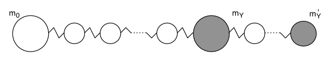
Figure 6: Spring system corresponding to the neutral gauge-boson sector of $SU(2)^{2}\times U(1)$ model with a brane kinetic term. $m_{0}\propto 1/\tilde{g}^{2}_{5W}$, $m_{Y}\propto 1/g^{2}_{Y}$, and $m^{\prime}_{Y}\propto 1/g^{\prime 2}_{Y}$ are larger than all of the other masses in the chain.

We now analyze a modified version of our warped-space bulk $SU(2)\times SU(2)\times U(1)$ model which includes a TeV brane $U(1)$ gauge kinetic term. This model provides a counter-example to our previous discussion in the sense that the bulk and brane kinetic $U(1)$ couplings will now appear separately in the calculation of the $\gamma$, $W$, and $Z$ couplings. The action for this model contains the term [34]

$$S_{\rm TeV}=\int_{R}^{R^{\prime}}dz\int d^{4}x\left\{-\dfrac{1}{4g^{\prime 2}_{Y}}\delta(z-R^{\prime}+0^{+})B_{\mu\nu}B_{\rho\lambda}\eta^{\mu\rho}\eta^{\nu\lambda}\right\}~{},$$ (127)

in addition to those given in eqn. (59).

The spring system corresponding to the neutral gauge boson sector in this case is shown in figure 6 and, as drawn, we will consider the system in the limit that $g^{2}_{Y}<g^{\prime 2}_{Y}$ or $m^{\prime}_{Y}<m_{Y}$. The zero mode corresponds to translation of the entire system, as before. The lightest non-zero mode again corresponds, roughly, to a “breathing” mode with masses $m_{0}$ and $m_{Y}$ oscillating slowly apart. To the extent $m^{\prime}_{Y}$ is not negligible, however, we expect that the distance between $m_{Y}$ and $m^{\prime}_{Y}$ will oscillate slowly as well. In this case, it is not possible to replace all of the $U(1)$ masses by a single effective mass – as in eqn. (3). As we will see, this will lead to potentially large corrections to the electroweak parameters of order $(m^{\prime}_{Y}/m_{Y})^{2}$.

The calculations proceed analogously to those in section 4, see appendix C. We will perform the calculation perturbatively in the coupling $g^{\prime 2}_{Y}$, so it will be convenient to define

$$\eta^{\prime}\equiv\dfrac{\tilde{g}_{5Y}^{2}}{g^{\prime 2}_{Y}}\dfrac{2}{b}\propto\dfrac{m^{\prime}_{Y}}{m_{Y}}~{}.$$ (128)

For ideally delocalized fermions, we find

$$e = \sqrt{\dfrac{2}{b}}\tilde{g}_{5W}s_{W}\left[1-\frac{3}{16}\frac{2}{b}+\dfrac{1}{4}\dfrac{s_{W}^{2}}{c_{W}^{2}}\dfrac{\tilde{g}_{5W}^{2}}{\tilde{g}_{5Y}^{2}}\eta^{\prime 2}+\cdots\right],$$ (129)

$$g^{W}_{W} = \sqrt{\dfrac{2}{b}}\tilde{g}_{5W}\left[1-\frac{3}{16}\frac{2}{b}+\cdots\right],$$ (130)

$$g^{Z}_{W} = \sqrt{\dfrac{2}{b}}\tilde{g}_{5W}c_{W}\left[1-\frac{3}{16}\frac{2}{b}-\dfrac{1}{4}\dfrac{s_{W}^{4}}{c_{W}^{4}}\dfrac{\tilde{g}_{5W}^{2}}{\tilde{g}_{5Y}^{2}}\eta^{\prime 2}+\cdots\right],$$ (131)

$$g^{Z}_{Y} = -\sqrt{\dfrac{2}{b}}\tilde{g}_{5W}\dfrac{s_{W}^{2}}{c_{W}}\left[1-\frac{3}{16}\frac{2}{b}-\dfrac{1}{4}\dfrac{s_{W}^{4}}{c_{W}^{4}}\dfrac{\tilde{g}_{5W}^{2}}{\tilde{g}_{5Y}^{2}}\eta^{\prime 2}+\cdots\right].$$ (132)

Note the non-trivial dependence on $\eta^{\prime}$, and hence dependence on $\tilde{g}_{5Y}$ beyond that encoded in the splitting between $M^{2}_{W}$ and $M^{2}_{Z}$. These couplings result in non-vanishing $\alpha S$ and $\alpha T$,

$$\alpha S = -2\dfrac{s^{4}}{c^{2}}\dfrac{\tilde{g}_{5W}^{2}}{\tilde{g}_{5Y}^{2}}\eta^{\prime 2},$$ (133)

$$\alpha T = -\frac{1}{2}\dfrac{s^{4}}{c^{4}}\dfrac{\tilde{g}_{5W}^{2}}{\tilde{g}_{5Y}^{2}}\eta^{\prime 2},$$ (134)

even for the case of ideal delocalization. This is consistent with the results of [34] for Higgsless models with localized fermions which are not precisely “case 1,” as defined in [16].

7 Conclusions

In this paper we have discussed ideal delocalization of fermions in a bulk $SU(2)\times SU(2)\times U(1)$ Higgsless model with a flat or warped extra dimension. So as to make an extra dimensional interpretation possible, both the weak and hypercharge properties of the fermions were delocalized, with the left-handed $U(1)_{Y}$ current of fermion being correlated with the $SU(2)_{W}$ current. We showed that (up to corrections of subleading order) ideal fermion delocalization yields vanishing precision electroweak corrections in this continuum model, as found in the corresponding theory space models based on deconstruction. Furthermore, we have shown that the phenomenology of these models is – to this order – equivalent to that of a simpler $SU(2)\times SU(2)$ model. The leading phenomenological constraints on Higgsless models with ideal delocalization come from studies of the constraints arising from deviations of the $ZWW$ vertex, a topic investigated in [30].

Appendix A Explicit Calculations in Warped Space

This appendix includes the explicit calculations of the normalization constants for the gauge boson wave functions.

A.1 $W$ profile normalization constants

It is convenient to define

$$f_{WN}(z) \equiv 1-\frac{1}{2}(M_{W}z)^{2}\left(\ln\frac{z}{R}-\frac{1}{2}\right)+\frac{1}{16}(M_{W}z)^{4}\ln\frac{z}{R}+\cdots,$$ (135)

$$f_{WD}(z) \equiv M_{W}zJ_{1}(M_{W}z)$$ (136)

$$= \frac{1}{2}(M_{W}z)^{2}-\frac{1}{16}(M_{W}z)^{4}+\cdots.$$

Both functions satisfy differential equation eqn. (70). The function $f_{WN}$ satisfies the Neumann condition at $z=R$, while $f_{WD}$ satisfies the Dirichlet condition. By using these functions we can express the $W$ mode functions satisfying the boundary conditions Eqs.(73) and (75) as

$$\chi_{W}^{A}(z)=C_{W}^{A}f_{WN}(z),\qquad\chi_{W}^{B}(z)=C_{W}^{B}f_{WD}(z),$$ (137)

where $C_{W}^{A}$ and $C_{W}^{B}$ are normalization constants. The boundary condition eqn. (74) then reads

$$0=\left(\begin{array}[]{cr}f_{WN}(z=R^{\prime})&-f_{WD}(z=R^{\prime})\\ f^{\prime}_{WN}(z=R^{\prime})&f^{\prime}_{WD}(z=R^{\prime})\end{array}\right)\left(\begin{array}[]{c}C_{W}^{A}\\ C_{W}^{B}\end{array}\right),$$ (138)

with $f^{\prime}_{WN}$ and $f^{\prime}_{WD}$ being defined as $f^{\prime}_{WN}(z)\equiv\partial_{z}f_{N}(z)$ and $f^{\prime}_{WD}(z)\equiv\partial_{z}f_{D}(z)$. In order to obtain non-zero $C_{W}^{A,B}$ the determinant of the matrix in eqn. (138) should vanish,

$$0=\dfrac{f^{\prime}_{WD}(R^{\prime})}{f^{\prime}_{WN}(R^{\prime})}+\dfrac{f_{WD}(R^{\prime})}{f_{WN}(R^{\prime})}.$$ (139)

From the definitions of $f_{WN}(z)$ and $f_{WD}(z)$ we can write the explicit expansions

$$f_{WN}(R^{\prime}) = 1-\frac{b}{4}(M_{W}R^{\prime})^{2}+\frac{1}{4}(M_{W}R^{\prime})^{2}+\frac{b}{32}(M_{W}R^{\prime})^{4}+\cdots,$$ (140)

$$f_{WD}(R^{\prime}) = \frac{1}{2}(M_{W}R^{\prime})^{2}-\frac{1}{16}(M_{W}R^{\prime})^{4}+\cdots,$$ (141)

$$R^{\prime}f^{\prime}_{WN}(R^{\prime}) = -\frac{b}{2}(M_{W}R^{\prime})^{2}+\frac{b}{8}(M_{W}R^{\prime})^{4}+\cdots,$$ (142)

$$R^{\prime}f^{\prime}_{WD}(R^{\prime}) = (M_{W}R^{\prime})^{2}-\frac{1}{4}(M_{W}R^{\prime})^{4}+\cdots~{}.$$ (143)

It is now straightforward to determine the $W$ mass as a function of the warp factor $b$ from eqn. (139). We obtain

$$(M_{W}R^{\prime})^{2}=\frac{2}{b}\left[1+\frac{3}{8}\frac{2}{b}+\cdots\right].$$ (144)

Note here $M_{W}$ is suppressed by $1/b$.

From Eqs.(142) and (143) we see

$$\dfrac{f^{\prime}_{WN}(R^{\prime})}{f^{\prime}_{WD}(R^{\prime})}=-\frac{b}{2}+{\cal O}\left(\frac{1}{b}\right).$$ (145)

Comparing this expression with eqn. (138) we find

$$C_{W}^{B}=C_{W}^{A}\left(\frac{b}{2}+{\cal O}\left(\frac{1}{b}\right)\right).$$ (146)

We now turn to the normalization condition eqn. (85). It is straightforward to show

$$\int_{R}^{R^{\prime}}dz\dfrac{1}{z}\left|f_{WN}(z)\right|^{2}=\frac{b}{2}-\frac{7}{16}+{\cal O}\left(\frac{1}{b}\right),$$ (147)

$$\int_{R}^{R^{\prime}}dz\dfrac{1}{z}\left|f_{WD}(z)\right|^{2}=\frac{1}{16}\left(\dfrac{2}{b}\right)^{2}+{\cal O}\left(\dfrac{1}{b^{3}}\right),$$ (148)

where we used eqn. (144) so as to express the results solely in terms of $b$. Finally, we can calculate the normalization constants $C_{W}^{A,B}$,

$$C_{W}^{A}=\sqrt{\dfrac{2}{b}}\tilde{g}_{5W}\left[1+\frac{3}{16}\frac{2}{b}+\cdots\right]\approx C_{W}^{B}\,\frac{2}{b}~{}.$$ (149)

A.2 $Z$ profile normalization constants

The $Z$ profile can be studied in a similar manner. We define

$$f_{ZN}(z) \equiv 1-\frac{1}{2}(M_{Z}z)^{2}\left(\ln\frac{z}{R}-\frac{1}{2}\right)+\frac{1}{16}(M_{Z}z)^{4}\ln\frac{z}{R}+\cdots,$$ (150)

$$f_{ZD}(z) \equiv M_{Z}zJ_{1}(M_{Z}z)$$ (151)

$$= \frac{1}{2}(M_{Z}z)^{2}-\frac{1}{16}(M_{Z}z)^{4}+\cdots.$$

Both functions satisfy differential equation eqn. (71). The function $f_{ZN}$ satisfies the Neumann condition at $z=R$, while $f_{ZD}$ satisfies the Dirichlet condition.

The Neumann condition, eqn. (76), at $z=R$ fixes the form of $\chi_{Z}^{A}$,

$$\chi_{Z}^{A}(z)=C_{Z}^{A}f_{ZN}(z),$$ (152)

while we express $\chi_{Z}^{B}$ as a linear combination of two independent solutions,

$$\chi_{Z}^{B}(z)=C_{Z}^{B}\left[f_{ZD}(z)+r_{B}f_{ZN}(z)\right],$$ (153)

with $r_{B}$ being a constant. The mode function in the Y-branch ($\chi_{Z}^{Y}$) can also be expressed as

$$\chi_{Z}^{Y}(z)=C_{Z}^{Y}\left[f_{ZD}(z)+r_{Y}f_{ZN}(z)\right],$$ (154)

where the Neumann condition, eqn. (80), at $z=R^{\prime}$ determines the constant $r_{Y}$,

$$r_{Y}=\dfrac{2}{b}.$$ (155)

The constant $r_{B}$ is determined from the boundary condition at $z=R^{\prime}$, eqn. (77), which may be written

$$0=\left(\begin{array}[]{cr}f_{ZN}(R^{\prime})&-f_{ZD}(R^{\prime})-r_{B}f_{ZN}(R^{\prime})\\ f^{\prime}_{ZN}(R^{\prime})&f^{\prime}_{ZD}(R^{\prime})+r_{B}f^{\prime}_{ZN}(R^{\prime})\end{array}\right)\left(\begin{array}[]{c}C_{Z}^{A}\\ C_{Z}^{B}\end{array}\right).$$ (156)

Again the determinant should vanish. We thus find

$$0=\dfrac{f^{\prime}_{ZD}(R^{\prime})}{f^{\prime}_{ZN}(R^{\prime})}+\dfrac{f_{ZD}(R^{\prime})}{f_{ZN}(R^{\prime})}+2r_{B}.$$ (157)

It is easy to show

$$\dfrac{f^{\prime}_{ZD}(R^{\prime})}{f^{\prime}_{ZN}(R^{\prime})}=-\dfrac{2}{b}.$$ (158)

The calculation of $f_{ZD}(R^{\prime})/f_{ZN}(R^{\prime})$ is a little more involved. We introduce the weak mixing angle defined by the $M_{W}/M_{Z}$ ratio,

$$c_{W}^{2}\equiv\dfrac{M_{W}^{2}}{M_{Z}^{2}},\qquad s_{W}^{2}=1-c_{W}^{2}.$$ (159)

Using eqn. (144), the $M_{Z}R^{\prime}$ terms in $f_{ZD}(R^{\prime})/f_{ZN}(R^{\prime})$ can be re-expressed in terms of $b$ and $c_{W}^{2}$, yielding

$$\dfrac{f_{ZD}(R^{\prime})}{f_{ZN}(R^{\prime})}=\dfrac{1}{c_{W}^{2}-s_{W}^{2}}\dfrac{2}{b}\left[1-\dfrac{3}{4}\dfrac{s_{W}^{2}}{c_{W}^{2}-s_{W}^{2}}\dfrac{2}{b}+\cdots\right].$$ (160)

Combining Eqs. (157), (158) and (160), we find

$$r_{B}=-\dfrac{s_{W}^{2}}{c_{W}^{2}-s_{W}^{2}}\dfrac{2}{b}\left[1-\frac{3}{8}\dfrac{1}{c_{W}^{2}-s_{W}^{2}}\dfrac{2}{b}+\cdots\right].$$ (161)

This, in turn, leads to a relation between $C^{A}_{Z}$ and $C^{B}_{Z}$. From eqn. (156) we can read off the equation

$$0=C_{Z}^{A}+C_{Z}^{B}\left(r_{B}+\dfrac{f^{\prime}_{ZD}(R^{\prime})}{f^{\prime}_{ZN}(R^{\prime})}\right).$$ (162)

Combining this with eqn. (158) and eqn. (161), we find

$$C_{Z}^{B}r_{B}=-\dfrac{s_{W}^{2}}{c_{W}^{2}}\left[1-\dfrac{3}{8c_{W}^{2}}\dfrac{2}{b}+\cdots\right]C_{Z}^{A}.$$ (163)

The last piece we need before separately determining $C^{A}_{Z}$ and $C^{B}_{Z}$ may be obtained by considering the mode function in the $Y$ branch $\chi_{Z}^{Y}(z)$, eqn. (154). The boundary condition eqn. (78) determines the constant $C_{Z}^{Y}$,

$$C_{Z}^{Y}r_{Y}=C_{Z}^{B}r_{B}=-\dfrac{s_{W}^{2}}{c_{W}^{2}}\left[1-\dfrac{3}{8c_{W}^{2}}\dfrac{2}{b}+\cdots\right]C_{Z}^{A}.$$ (164)

Combining the boundary conditions eqn. (78) and eqn. (79), we also find an expression for the brane kinetic term $1/g_{Y}^{2}$,

$$\dfrac{1}{g_{Y}^{2}}=-\dfrac{1}{\tilde{g}_{5W}^{2}}\left.\dfrac{\partial_{z}\chi_{z}^{B}(z)}{M_{Z}^{2}R\chi_{Z}^{B}(z)}\right|_{z=R}-\dfrac{1}{\tilde{g}_{5Y}^{2}}\left.\dfrac{\partial_{z}\chi_{z}^{Y}(z)}{M_{Z}^{2}R\chi_{Z}^{Y}(z)}\right|_{z=R}.$$ (165)

Plugging eqn. (153) and eqn. (154) in eqn. (165) we obtain

$$\dfrac{1}{g_{Y}^{2}}=-\dfrac{1}{r_{B}}\dfrac{1}{\tilde{g}_{5W}^{2}}-\dfrac{1}{r_{Y}}\dfrac{1}{\tilde{g}_{5Y}^{2}}.$$ (166)

Substituting eqn. (155) and eqn. (161) in this expression, we further see

$$\dfrac{1}{g_{Y}^{2}}+\dfrac{1}{\tilde{g}_{5Y}^{2}}\dfrac{b}{2}=\dfrac{1}{\tilde{g}_{5W}^{2}}\dfrac{b}{2}\dfrac{c_{W}^{2}-s_{W}^{2}}{s_{W}^{2}}\left[1+\frac{3}{8}\dfrac{1}{c_{W}^{2}-s_{W}^{2}}\frac{2}{b}+\cdots\right].$$ (167)

Note that this particular combination of $g_{Y}$ and $\tilde{g}_{5Y}$ depends only on the bulk $SU(2)$ coupling.

We are now ready to determine the normalization constant $C_{Z}^{A}$ from eqn. (86). This equation contains both an explicit dependence on the bulk $U(1)$ coupling $\tilde{g}_{5Y}$ in its third term and an implicit dependence on $\tilde{g}_{5Y}$ in its fourth term, through the $g_{Y}^{2}$ value calculated in eqn. (167). However, these two $\tilde{g}_{5Y}$ dependences cancel at the order we are working to, as we shall now see. First, we note that

$$\int_{R}^{R^{\prime}}dz\frac{1}{z}\left|f_{ZN}(z)+\frac{1}{r_{Y}}f_{ZD}(z)\right|^{2}=\frac{b}{2}+{\cal O}\left(\frac{1}{b}\right).$$ (168)

The absence of a $b^{0}$ term in eqn. (168) reflects the approximate flatness of the mode function $\chi_{Z}^{Y}(z)$. The third and fourth terms of eqn. (86) therefore yield

$$\int_{R}^{R^{\prime}}\!\!dz\dfrac{1}{z\tilde{g}_{5Y}^{2}}\left|\chi^{Y}_{Z}(z)\right|^{2}+\dfrac{1}{g_{Y}^{2}}\left|\chi^{Y}_{Z}(R)\right|^{2}=(C_{Z}^{Y})^{2}r_{Y}^{2}\left(\dfrac{1}{g_{Y}^{2}}+\dfrac{1}{\tilde{g}_{5Y}^{2}}\dfrac{b}{2}\right).$$ (169)

Inserting Eqs. (155) and (167) in the RHS of this expression, confirms the cancellation of the $\tilde{g}_{5Y}$ dependence at this order.

To complete the calculation, we first compute the remaining terms in eqn. (86)

$$\int_{R}^{R^{\prime}}dz\frac{1}{z}|f_{ZN}(z)|^{2}=\frac{b}{2}-\frac{1}{2}\dfrac{1}{c_{W}^{2}}+\frac{1}{16}\dfrac{1}{c_{W}^{4}}+\cdots,$$ (170)

$$\int_{R}^{R^{\prime}}dz\frac{1}{z}\left|f_{ZN}(z)+\frac{1}{r_{B}}f_{ZD}(z)\right|^{2}=\frac{b}{2}-\frac{1}{2}\dfrac{1}{s_{W}^{2}}+\frac{1}{16}\dfrac{1}{s_{W}^{4}}+\cdots.$$ (171)

We then obtain the normalization constants as

$$C^{A}_{Z}=\sqrt{\dfrac{2}{b}}\tilde{g}_{5W}c_{W}\left[1+\dfrac{3}{16}\dfrac{2-c_{W}^{2}}{c_{W}^{2}}\dfrac{2}{b}+\cdots\right],$$ (172)

and

$$C^{B}_{Z}r_{B}=-\sqrt{\dfrac{2}{b}}\tilde{g}_{5W}\dfrac{s_{W}^{2}}{c_{W}}\left[1-\dfrac{3}{16}\dfrac{2}{b}+\cdots\right].$$ (173)

We emphasize once again that these normalization constants $C_{Z}^{A}$, $C_{Z}^{B}$ are insensitive to the bulk $U(1)$ coupling $\tilde{g}_{5Y}$. The mode functions $\chi_{Z}^{A}$ and $\chi_{Z}^{B}$ are thus identical with those of the simpler $SU(2)\times SU(2)$ model without a bulk $U(1)$ gauge field.

Appendix B KK-mode contribution to $\Delta\rho-\alpha T$ in flat space

In this appendix we restrict ourselves to the $g_{Y}\to 0$ limit; extension to finite $g_{Y}$ is straightforward.

In the flat-space model we have a series of neutral KK-modes,

$$\chi_{Z(n)}(y)\propto\left\{\begin{array}[]{lc}0&\mbox{for $y<2\pi R$},\\ C_{Z(n)}\sin\left(\dfrac{2n-1}{2R}(y-2\pi R)\right)&\mbox{for $y>2\pi R$},\end{array}\right.$$ (174)

in addition to the neutral KK-modes which are degenerate with the charged KK modes in the $g_{Y}\to 0$ limit. Since the KK-modes of eq.(174) overlap with the hypercharge current distribution eq.(48), we need to consider possible contributions [16] of these KK modes to $\Delta\rho-\alpha T$, i.e. to four-fermion processes at low energies. However, investigating the coupling of these KK-modes to the fermion $U(1)$ current, we find

$$g^{Z(n)}_{Y}=\dfrac{4}{\pi}\dfrac{1-(-1)^{n}}{2n-1}C_{Z(n)}(M_{W}\pi R)^{2},$$ (175)

with

$$C_{Z(n)}=\sqrt{\dfrac{2g_{5Y}^{2}}{\pi R}}.$$ (176)

Therefore, contributions from these KK-modes are suppressed by $(M_{W}\pi R)^{4}$,

$$\dfrac{(g^{Z(n)}_{Y})^{2}}{M_{Z(n)}^{2}}\propto(M_{W}\pi R)^{4}$$ (177)

and are negligible to the order we are working.

Appendix C Calculations with a TeV Brane $U(1)$ gauge kinetic term

In this appendix, we consider the effect of adding a TeV brane $U(1)$ gauge kinetic term

$$S_{\rm TeV}=\int_{R}^{R^{\prime}}dz\int d^{4}x\left\{-\dfrac{1}{4g^{\prime 2}_{Y}}\delta(z-R^{\prime}+0^{+})B_{\mu\nu}B_{\rho\lambda}\eta^{\mu\rho}\eta^{\nu\lambda}\right\}~{}.$$ (178)

to the action eqn. (59) [34]. We perform the calculation in an expansion in powers of

$$\eta^{\prime}\equiv\dfrac{\tilde{g}_{5Y}^{2}}{g^{\prime 2}_{Y}}\dfrac{2}{b}~{}.$$ (179)

In the following calculations, we neglect ${\cal O}(1/b^{2})$, ${\cal O}(\eta^{\prime 3})$, ${\cal O}(\eta^{\prime}/b)$ contributions to the fermion couplings – we only retain terms which suffice to calculate these couplings, and therefore $\alpha S$ and $\alpha T$, to ${\cal O}(1/b)$ and ${\cal O}(\eta^{\prime 2})$.

Because the charged sector of this model is independent of $\eta^{\prime}$, both the $W$ profile and the profile of an ideally delocalized fermion – and therefore the results of sections 4.2.1 and 4.2.4 – are unaltered.

The presence of the TeV brane gauge kinetic action eqn. (178) modifies the boundary condition of $\chi_{Z}^{Y}$ eqn. (80) and the normalization conditions of the $Z$ and photon mode functions eqn. (86) and eqn. (4.1),

$$0=\left.\dfrac{1}{\tilde{g}_{5Y}^{2}}\partial_{z}\chi_{Z}^{Y}(z)\right|_{z=R^{\prime}}-M_{Z}^{2}\dfrac{R^{\prime}}{g^{\prime 2}_{Y}}\left.\chi_{Z}^{Y}(z)\right|_{z=R^{\prime}},$$ (180)

$$1 = \int_{R}^{R^{\prime}}\!\!dz\dfrac{1}{z\tilde{g}_{5W}^{2}}\left|\chi^{A}_{Z}(z)\right|^{2}+\int_{R}^{R^{\prime}}\!\!dz\dfrac{1}{z\tilde{g}_{5W}^{2}}\left|\chi^{B}_{Z}(z)\right|^{2}+\int_{R}^{R^{\prime}}\!\!dz\dfrac{1}{z\tilde{g}_{5Y}^{2}}\left|\chi^{Y}_{Z}(z)\right|^{2}$$ (181)

$$\qquad\qquad+\dfrac{1}{g_{Y}^{2}}\left|\chi^{Y}_{Z}(R)\right|^{2}+\dfrac{1}{g_{Y}^{\prime 2}}\left|\chi^{Y}_{Z}(R^{\prime})\right|^{2},$$

$$1 = \int_{R}^{R^{\prime}}\!\!dz\dfrac{1}{z\tilde{g}_{5W}^{2}}\left|\chi^{A}_{\gamma}(z)\right|^{2}+\int_{R}^{R^{\prime}}\!\!dz\dfrac{1}{z\tilde{g}_{5W}^{2}}\left|\chi^{B}_{\gamma}(z)\right|^{2}+\int_{R}^{R^{\prime}}\!\!dz\dfrac{1}{z\tilde{g}_{5Y}^{2}}\left|\chi^{Y}_{\gamma}(z)\right|^{2}$$ (182)

$$\qquad\qquad+\dfrac{1}{g_{Y}^{2}}\left|\chi^{Y}_{\gamma}(R)\right|^{2}+\dfrac{1}{g_{Y}^{\prime 2}}\left|\chi^{Y}_{\gamma}(R^{\prime})\right|^{2}.$$

The analysis of the $Z$ mode wavefunction proceeds as in section 4.2.2 and appendix A, with some expressions now depending on $\eta^{\prime}$. Specifically,

$$r_{Y}=\dfrac{2}{b}\left[1-\eta^{\prime}+\dfrac{c_{W}^{2}-s_{W}^{2}}{2c_{W}^{2}}\eta^{\prime 2}+\cdots\right]~{},$$ (183)

eqn. (167) is replaced by

$$\dfrac{1}{g_{Y}^{2}}+\dfrac{1}{\tilde{g}_{5Y}^{2}}\dfrac{b}{2}+\dfrac{1}{g_{Y}^{\prime 2}}=\dfrac{1}{\tilde{g}_{5W}^{2}}\dfrac{b}{2}\dfrac{c_{W}^{2}-s_{W}^{2}}{s_{W}^{2}}\left[1+\frac{3}{8}\dfrac{1}{c_{W}^{2}-s_{W}^{2}}\frac{2}{b}\right]-\dfrac{1}{2c_{W}^{2}}\dfrac{1}{\tilde{g}_{5Y}^{2}}\dfrac{b}{2}\eta^{\prime 2}+\cdots~{},$$ (184)

eqns.(168) and (169) are, respectively, replaced by

$$\int_{R}^{R^{\prime}}dz\frac{1}{z}\left|f_{ZN}(z)+\frac{1}{r_{Y}}f_{ZD}(z)\right|^{2}=\frac{b}{2}\left[1+{\cal O}\left(\dfrac{\eta^{\prime}}{b},\dfrac{1}{b^{2}}\right)\right],$$ (185)

and

$$\int_{R}^{R^{\prime}}\!\!dz\dfrac{1}{z\tilde{g}_{5Y}^{2}}\left|\chi^{Y}_{Z}(z)\right|^{2}+\dfrac{1}{g_{Y}^{2}}\left|\chi^{Y}_{Z}(R)\right|^{2}+\dfrac{1}{g_{Y}^{\prime 2}}\left|\chi^{Y}_{Z}(R^{\prime})\right|^{2}$$ (186)

$$=(C_{Z}^{Y})^{2}r_{Y}^{2}\left(\dfrac{1}{g_{Y}^{2}}+\dfrac{1}{\tilde{g}_{5Y}^{2}}\dfrac{b}{2}+\dfrac{1}{g_{Y}^{\prime 2}}+\dfrac{1}{c_{W}^{2}}\dfrac{1}{\tilde{g}_{5Y}^{2}}\dfrac{b}{2}\eta^{\prime 2}+\cdots\right).$$

Ultimately, the expression for the normalization constants eqns. (100) and (101) become, respectively,

$$C^{A}_{Z}=\sqrt{\dfrac{2}{b}}\tilde{g}_{5W}c_{W}\left[1+\dfrac{3}{16}\dfrac{2-c_{W}^{2}}{c_{W}^{2}}\dfrac{2}{b}-\dfrac{1}{4}\dfrac{s_{W}^{4}}{c_{W}^{4}}\dfrac{\tilde{g}_{5W}^{2}}{\tilde{g}_{5Y}^{2}}\eta^{\prime 2}+\cdots\right]~{},$$ (187)

and

$$C^{B}_{Z}r_{B}=-\sqrt{\dfrac{2}{b}}\tilde{g}_{5W}\dfrac{s_{W}^{2}}{c_{W}}\left[1-\dfrac{3}{16}\dfrac{2}{b}-\dfrac{1}{4}\dfrac{s_{W}^{4}}{c_{W}^{4}}\dfrac{\tilde{g}_{5W}^{2}}{\tilde{g}_{5Y}^{2}}\eta^{\prime 2}+\cdots\right].$$ (188)

Note here that the normalization of the $Z$ mode function in $SU(2)$ branches ($C_{Z}^{A,B}$) is sensitive to the coupling in the $U(1)$ branch ($\tilde{g}_{5Y}$) at the order of $\eta^{\prime 2}$.

For the $\gamma$ wavefunction, section 4.2.3, we find that eqn. (103) and eqn. (104) are replaced by

$$1=C_{\gamma}^{2}\left(\dfrac{2}{\tilde{g}_{5W}^{2}}\dfrac{b}{2}+\dfrac{1}{\tilde{g}_{5Y}^{2}}\dfrac{b}{2}+\dfrac{1}{g_{Y}^{2}}+\dfrac{1}{g_{Y}^{\prime 2}}\right),$$ (189)

and

$$C_{\gamma}=\sqrt{\dfrac{2}{b}}\tilde{g}_{5W}s_{W}\left(1-\dfrac{3}{16}\frac{2}{b}+\dfrac{1}{4}\dfrac{s_{W}^{2}}{c_{W}^{2}}\dfrac{\tilde{g}_{5W}^{2}}{\tilde{g}_{5Y}^{2}}\eta^{\prime 2}+\cdots\right).$$ (190)

Again observe that the normalization of the $\gamma$ mode function ($C_{\gamma}$) is sensitive to the coupling of the $U(1)$ branch ($\tilde{g}_{5Y}$) at this order.

Calculating the couplings of an ideally delocalized fermion, we find the results quoted in eqns. (129) – (134).

References

- [1] C. Csaki, C. Grojean, H. Murayama, L. Pilo and J. Terning, Gauge theories on an interval: Unitarity without a Higgs, Phys. Rev. D 69, 055006 (2004) [arXiv:hep-ph/0305237].
- [2] P. W. Higgs, Broken symmetries, massless particles and gauge fields, Phys. Lett. 12 (1964) 132–133.
- [3] K. Agashe, A. Delgado, M. J. May and R. Sundrum, RS1, Custodial Isospin and Precision Tests, JHEP 0308, 050 (2003) [arXiv:hep-ph/0308036].
- [4] C. Csaki, C. Grojean, L. Pilo, and J. Terning, Towards a realistic model of higgsless electroweak symmetry breaking, Phys. Rev. Lett. 92 (2004) 101802, [hep-ph/0308038].
- [5] R. Sekhar Chivukula, D. A. Dicus, and H.-J. He, Unitarity of compactified five dimensional yang-mills theory, Phys. Lett. B525 (2002) 175–182, [hep-ph/0111016].
- [6] R. S. Chivukula and H.-J. He, Unitarity of deconstructed five-dimensional yang-mills theory, Phys. Lett. B532 (2002) 121–128, [hep-ph/0201164].
- [7] R. S. Chivukula, D. A. Dicus, H.-J. He, and S. Nandi, Unitarity of the higher dimensional standard model, Phys. Lett. B562 (2003) 109–117, [hep-ph/0302263].
- [8] H.-J. He, Higgsless deconstruction without boundary condition, arXiv:hep-ph/0412113.
- [9] R. Foadi, S. Gopalakrishna, and C. Schmidt, Higgsless electroweak symmetry breaking from theory space, JHEP 03 (2004) 042, [hep-ph/0312324].
- [10] J. Hirn and J. Stern, The role of spurions in Higgs-less electroweak effective theories, Eur. Phys. J. C 34, 447 (2004) [arXiv:hep-ph/0401032].
- [11] R. Casalbuoni, S. De Curtis and D. Dominici, Moose models with vanishing S parameter, Phys. Rev. D 70 (2004) 055010 [arXiv:hep-ph/0405188].
- [12] R. S. Chivukula, E. H. Simmons, H. J. He, M. Kurachi and M. Tanabashi, The structure of corrections to electroweak interactions in Higgsless models, Phys. Rev. D 70 (2004) 075008 [arXiv:hep-ph/0406077].
- [13] M. Perelstein, Gauge-assisted technicolor?, JHEP 10 (2004) 010, [hep-ph/0408072].
- [14] R. S. Chivukula, E. H. Simmons, H.-J. He, M. Kurachi, and M. Tanabashi, Universal non-oblique corrections in higgsless models and beyond, Phys. Lett. B603 (2004) 210–218, [hep-ph/0408262].
- [15] H. Georgi, Fun with Higgsless theories, Phys. Rev. D 71, 015016 (2005) [arXiv:hep-ph/0408067].
- [16] R. Sekhar Chivukula, E. H. Simmons, H. J. He, M. Kurachi and M. Tanabashi, Electroweak corrections and unitarity in linear moose models, Phys. Rev. D 71 (2005) 035007 [arXiv:hep-ph/0410154].
- [17] N. Arkani-Hamed, A. G. Cohen, and H. Georgi, (de)constructing dimensions, Phys. Rev. Lett. 86 (2001) 4757–4761, [hep-th/0104005].
- [18] C. T. Hill, S. Pokorski, and J. Wang, Gauge invariant effective lagrangian for kaluza-klein modes, Phys. Rev. D64 (2001) 105005, [hep-th/0104035].
- [19] M. E. Peskin and T. Takeuchi, Estimation of oblique electroweak corrections, Phys. Rev. D46 (1992) 381–409.
- [20] G. Altarelli and R. Barbieri, Vacuum polarization effects of new physics on electroweak processes, Phys. Lett. B253 (1991) 161–167.
- [21] G. Altarelli, R. Barbieri, and S. Jadach, Toward a model independent analysis of electroweak data, Nucl. Phys. B369 (1992) 3–32.
- [22] H. Georgi, A tool kit for builders of composite models, Nucl. Phys. B266 (1986) 274.
- [23] R. Barbieri, A. Pomarol, R. Rattazzi and A. Strumia, Nucl. Phys. B 703, 127 (2004) [arXiv:hep-ph/0405040].
- [24] G. Cacciapaglia, C. Csaki, C. Grojean and J. Terning, Curing the ills of Higgsless models: The S parameter and unitarity, Phys. Rev. D 71 (2005) 035015 [arXiv:hep-ph/0409126].
- [25] R. Foadi, S. Gopalakrishna and C. Schmidt, Effects of fermion localization in Higgsless theories and electroweak constraints, Phys. Lett. B 606 (2005) 157 [arXiv:hep-ph/0409266].
- [26] R. Foadi and C. Schmidt, An Effective Higgsless Theory: Satisfying Electroweak Constraints and a Heavy Top Quark, arXiv:hep-ph/0509071.
- [27] R. S. Chivukula, E. H. Simmons, H. J. He, M. Kurachi and M. Tanabashi, Deconstructed Higgsless models with one-site delocalization, Phys. Rev. D 71, 115001 (2005) [arXiv:hep-ph/0502162].
- [28] R. Casalbuoni, S. De Curtis, D. Dolce and D. Dominici, Playing with fermion couplings in Higgsless models, Phys. Rev. D 71, 075015 (2005) [arXiv:hep-ph/0502209].
- [29] R. Sekhar Chivukula, E. H. Simmons, H. J. He, M. Kurachi and M. Tanabashi, Ideal fermion delocalization in Higgsless models, Phys. Rev. D 72, 015008 (2005) [arXiv:hep-ph/0504114].
- [30] R. S. Chivukula, E. H. Simmons, H. J. He, M. Kurachi and M. Tanabashi, Multi-gauge-boson vertices and chiral Lagrangian parameters in higgsless models with ideal fermion delocalization, arXiv:hep-ph/0508147.
- [31] A. Falkowski and H. D. Kim, “Running of gauge couplings in AdS(5) via deconstruction,” JHEP 0208, 052 (2002) [arXiv:hep-ph/0208058].
- [32] L. Randall, Y. Shadmi and N. Weiner, “Deconstruction and gauge theories in AdS(5),” JHEP 0301, 055 (2003) [arXiv:hep-th/0208120].
- [33] R. Sekhar Chivukula, E. H. Simmons, H. J. He, M. Kurachi and M. Tanabashi, to be published.
- [34] G. Cacciapaglia, C. Csaki, C. Grojean and J. Terning, Oblique corrections from Higgsless models in warped space, Phys. Rev. D 70, 075014 (2004) [arXiv:hep-ph/0401160].