Abstract

We discuss heavy quarkonium production through parton fragmentation, including a review of arguments for the factorization of high-$p_{T}$ particles into fragmentation functions for hadronic initial states. We investigate the further factorization of fragmentation functions in the NRQCD formalism, and argue that this requires a modification of NRQCD octet production matrix elements to include nonabelian phases, which makes them gauge invariant. We describe the calculation of uncanceled infrared divergences in fragmentation functions that must be factorized at NNLO, and verify that they are absorbed into the new, gauge invariant matrix elements.

PACS numbers: 12.38.Bx, 12.39.St, 13.87.Fh, 14.40Gx

1 Introduction

The production of bound states of heavy quark pairs played an historic role in the development of the Standard Model [1]. This subject has retained a continuing fascination, in part because it offers unique perspectives into the formation of QCD bound states. The first step in quarkonium production, the inclusive creation of a pair of charm or bottom quarks, is an essentially perturbative process. In particular, at high transverse momentum in hard-scattering processes, the dominant mechanism for the production of heavy quarkonium is the perturbative fragmentation of lighter partons, especially the gluon [2].

A basic result of perturbative QCD for the production of hadrons $H$ at high transverse momentum from the scattering of initial-state particles $A$ and $B$ is the factorization of universal fragmentation functions, [3, 4, 5, 6]

$$d\sigma_{A+B\to H+X}(p_{T})=\sum_{i}\;d\tilde{\sigma}_{A+B\to i+X}(p_{T}/z,\mu)\otimes D_{H/i}(z,m_{c},\mu)+{\mathcal{O}}(m_{H}^{2}/p_{T}^{2})\,.$$ (1)

Here, $\otimes$ represents a convolution in the momentum fraction $z$. The cross section $d\hat{\sigma}_{A+B\to i+X}$ includes all information on the incoming state, including convolutions with parton distributions when $A$ and $B$ are hadrons, at factorization scale $\mu$. We exhibit the $m_{c}$-dependence of the fragmentation function $D_{H/i}$ in anticipation of our interest in $H$ as a charm-anticharm bound state, for which the boundary condition for evolution is naturally taken at $\mu={\cal O}(m_{c})$.

The actual transformation of a heavy quark pair into a heavy quarkonium $H$ with momentum fraction $z$ from parton $i$ requires the introduction of fragmentation functions $D_{H/i}(z,\mu)$. This reasoning applies in principle to both charm and bottom quarks. For definiteness, we will generally refer to the heavy quark mass by $m_{c}$, and to the produced hadrons as $H=J/\psi$ etc., of mass $m_{H}\sim 2m_{c}$.

At moderate $z$ only the evolution, that is, the $\mu$-dependence, of the fragmentation function is computable perturbatively, with the remaining information encoded in some initial function $D_{H/g}(z,\mu_{0})$, where we may take $\mu_{0}\sim m_{H}$. The effective field theory nonrelativistic QCD (NRQCD), however, has been invoked to simplify the nonperturbative content of the fragmentation functions $D_{H/i}(z,\mu_{0})$, in terms of a few (or anyway finite number of) nonperturbative matrix elements.

The logic behind the application of NRQCD to fragmentation functions is readily summarized. One applies the NRQCD expansion in the relative velocity of the produced quark pair, assuming that a bound state will form only if this relative velocity is small to begin with. One then argues that the formation of the bound state is not affected by the exchange of soft gluons with other hard partons, only by exchanges between the quark and antiquark, and with the vacuum [7]. NRQCD then specifies a complementary factorization theorem, often written as

$$d\sigma_{A+B\to H+X}(p_{T})=\sum_{n}\;d\hat{\sigma}_{A+B\to c\bar{c}[n]+X}(p_{T})\,\langle{\mathcal{O}}^{H}_{n}\rangle\,,$$ (2)

where the ${\mathcal{O}}^{H}_{n}$ are universal NRQCD production operators, organized according to powers of the relative velocity of the $c\bar{c}$ state $[n]$, and their rotational and color quantum numbers. We will encounter explicit forms below.

Next, accepting that both (1) and (2) hold at high-$p_{T}$, the fragmentation function and NRQCD matrix elements are related by [8]

$$D_{H/i}(z,m_{c},\mu)=\sum_{n}\;d_{i\to c\bar{c}[n]}(z,\mu,m_{c})\,\langle{\mathcal{O}}^{H}_{n}\rangle\,,$$ (3)

where $d_{i\to c\bar{c}[n]}(z,\mu,m_{c})$ describes the evolution of an off-shell parton into a quark pair in state $[n]$, including logarithms of $\mu/m_{c}$. This formalism has been extensively applied to heavy quarkonium production [9, 10, 11, 12, 13, 14, 15, 16]. At the same time, it has been observed that the applicability of NRQCD to production processes has not been fully demonstrated [16, 17].

In this paper we revisit the formation of heavy quarkonia in fragmentation, with the aim of testing the relation (3). We will, however, first outline the proof of Eq. (1) in leptonic annihilation and hadronic scattering, emphasizing that the arguments that apply to light quark bound states apply as well to heavy quarks, with corrections suppressed by powers of the mass of the quark divided by the transverse momentum. While our arguments for the factorization of fragmentation functions will not actually cover new ground, we are aware of no other unified presentation of the steps leading to (1) for hadronic scattering in nonabelian gauge theories.

Once we have established (1), we can test NRQCD factorization in its more specific form, Eq. (3), which will simplify our analysis considerably. We study the factorization of the fragmentation functions into perturbative coefficient functions times NRQCD matrix elements, with evolution included in the former. We shed new light on the necessary cancellation of infrared divergences in the perturbative calculation of coefficient functions. In particular, we will show that to carry out such a factorization, it is useful to redefine conventional NRQCD production matrix elements, with the addition of extra gauge links, or Wilson lines, a process that we termed “gauge completion” in Ref. [17]. This modification renders the matrix elements gauge invariant.

Gauge completion is also necessary in order to absorb certain infrared divergences, beginning at next-to-next-to leading order (NNLO), that were not covered by the original arguments for NRQCD factorization. We should note that our NNLO infrared effects will appear only at order $\alpha_{s}^{3}$ in inclusive heavy quark pair production cross sections of the type calculated to order $\alpha_{s}^{2}$ in [18] (see also the corresponding two loop decay cross sections in [19]). Indeed we will encounter two loop corrections with a quark pair and an additional hard gluon in the final state. The calculation is only possible, of course, because we restrict ourselves to the infrared sector.

In any case, however, we are not yet able to prove Eq. (3) to all orders in perturbation theory. The basic results of this paper were outlined in [17]. Here, in addition to the arguments on factorization, we will provide rather complete details on the methods used to identify the relevant infrared behavior, and on the necessary two-loop calculations.

2 Factorization of Fragmentation Functions

2.1 Long-distance dynamics in high-$p_{T}$ production.

The analysis of hard scattering cross sections begins with the identification of leading regions in the momentum space integrals of perturbative amplitudes and phase space [5, 20, 21]. Regions in this multidimensional space are conveniently classified in cut diagram notation, in which graphical contributions to the amplitude are represented to the left of the final state, and contributions to the complex conjugate amplitude to the right. In the complex conjugate graphs the roles of final and initial states are reversed.

Because loop integrals are defined by contours in complex momentum space, it is only at momentum configurations where some subset of loop momenta are pinched that the contours are forced to or near mass-shell poles that correspond to long-distance behavior. These “pinch surfaces”, or subspaces, in turn can be classified according to their reduced diagrams, found by contracting off-shell lines to points.

The basic result is this. Any reduced diagram corresponding to a pinch surface can be interpreted as a physical process, in which each vertex can be assigned positions $x_{i}^{\mu}$ in space-time in such a way that if $x_{i}$ and $x_{j}$ are connected by line $h$ carrying nonzero momentum $p_{h}$, then

$$\Delta x_{ij}^{\mu}\equiv\left(x_{i}-x_{j}\right)^{\mu}=(x_{i}-x_{j})^{0}\,\beta_{h}^{\mu}\,,$$ (4)

where $\beta_{h}^{\mu}=p_{h}^{\mu}/p_{h}^{0}$ is the four-velocity of particle $h$. At a pinch surface, this relation can be imposed for every line and vertex of the reduced diagram. Consistency then requires that the sum of $\Delta x_{ij}$’s around any loop vanishes. This is enough to ensure that the reduced diagram does correspond to a physical picture, in which on-shell lines describe free, classical motion between the vertices. To this physical picture for finite-energy lines, lines with vanishing momenta may be attached in an arbitrary manner [20, 21].

The proof of the relationship between pinches in loop momentum space and physical pictures described by (4) is not difficult [20, 22, 23], but we shall not review it here. Its consequences, however, are important and easily drawn.

Let us apply the above considerations to the production of a hadron $H$, with momentum $P$, in the scattering of particles $A$ and $B$,

$$A(p_{A})+B(p_{B})\rightarrow H(\vec{P})+X\,.$$ (5)

We will assume that $P_{T}$ is a large scale, of the order of the center-of-mass energy, and far above the strong coupling scale $\Lambda_{\mathrm{Q}CD}$. The relevant reduced diagrams for this process are illustrated in cut diagram notation by Fig. 1 when $A$ and $B$ are a leptonic pair, and by Fig. 2 when $A$ and $B$ are strongly interacting (partons or physical hadrons).

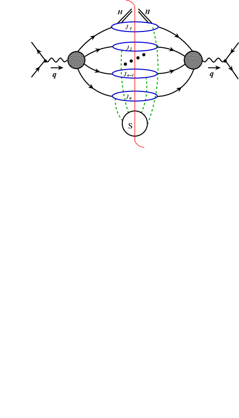
Figure 1: Reduced diagrams for high-$p_{T}$ particle production in leptonic annihilation.

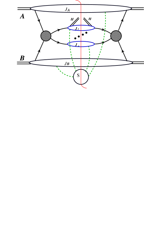
Figure 2: Reduced diagrams for high-$p_{T}$ particle production in hadronic collisions.

At the pinch surfaces, there is a single hard-scattering, labelled by a shaded circle, in the amplitude and its complex conjugate. For dilepton annihilation, Fig. 1, the hard scattering is the result of the decay of the (real or virtual) electroweak boson formed in the annihilation process. For the hadronic process, the hard scattering results from the collisions of a single parton from each of the colliding hadrons . Finite-energy partons emerge from the hard scatterings and connect to subdiagrams of on-shell collinear lines, the jets, $J_{i}$. All finite-energy particles of the final states are in one of these jets. In addition zero-momentum lines may be exchanged between the lines of the jets, and interact arbitrarily in a cut “soft subdiagram” $S$, consisting entirely of such lines. In effect, there are no final-state interactions involving finite momentum transfer in the reduced diagram for these processes. Thus, the total momentum of each jet is determined at the hard scattering, and the distributions of jet energies are calculable in perturbation theory. The essential observation to obtain this result is that once the parent partons of the jets emerge from the hard scattering, they separate at the speed of light, and subsequently cannot interact locally in any physical picture defined as above. The observed hadron $H$ appears in one of the jets .

We will not attempt a full review of power-counting analysis in the neighborhood an arbitrary reduced diagram of Figs. 1 and 2. It is worthwhile to recall, however, that we may characterize these regions of momentum space by introducing scaling variables, conventionally denoted $\lambda$, which control the relative rates at which components of loop momenta vanish near the pinch surfaces. In the terminology of [20], a leading region is one for which a vanishing region of loop momentum space near a pinch surface produces leading-power behavior. Such behavior is naturally associated with logarithmic singularities at the corresponding pinch surface.

For the pinch surfaces at hand, we assign to the $j$th jet a light-like vector in the jet direction, $\bar{n}_{j}^{\mu}$, $\bar{n}_{j}^{2}=0$, and an opposite-moving vector $n_{j}^{\mu}$, $n_{j}^{2}=0$, normalized such that $\bar{n}_{j}\cdot n_{j}=1$. For each jet, the combination of $\bar{n}_{j}$ and $n_{j}$ define a two-dimensional transverse space, which we will denote as ${\perp^{(j)}}$. The fundamental leading regions are characterized by a familiar scaling behavior for the loop momenta internal to jet $j$,

$${\rm loop}\ l\ {\rm in\ jet}\ j:\quad\left(n_{j}\cdot l\sim E_{j},\ \bar{n}_{j}\cdot l\sim\lambda E_{j},\ l_{\perp^{(j)}}\sim\lambda^{1/2}E_{j}\right)\,,$$ (6)

where $E_{j}$ is the energy characteristic of jet $j$, which we take to be of the order of the overall center-of-mass energy, denoted $Q$. In a similar notation, the scaling for soft loop momenta, internal to the soft subdiagram $S$ or flowing between $S$ and any of the jets, is

$${\rm soft\ loop}:\ k^{\mu}\sim\lambda\,Q\,.$$ (7)

In principle, the two scales $\lambda$ in Eq. (6) and (7) need not be the same. A complete discussion includes power counting for subdivergences, as some lines approach the mass shell faster than others [20, 21].

2.2 Jet-soft factorization

Arguments for the factorization of soft gluons from jets were given in some detail in Ref. [5] for $\rm e^{+}e^{-}$ annihilation. We review these arguments here, and discuss their extension to hadronic scattering. Jet-soft factorization is made possible by the singularity structure of loop integrals near pinch surfaces [4, 25]. Many of these results have been rederived in the language of soft-collinear effective theory [26, 27]. In graphical terms, the factorization is most clearly illustrated for leptonic annihilation, as in Fig. 1.

2.2.1 The soft approximation in leptonic annihilation

In Fig. 1 let us consider a loop momentum $k_{i}$, flowing from the soft subdiagram into jet $J_{j}$, through the hard scattering to another jet, and finally back to the soft subdiagram. We will examine poles in the integral near $k_{i}^{\mu}=0$ due to the denominators of $J_{j}$. For definiteness, we assume the $k_{i}$ loop is in the amplitude.

The soft momentum appears in propagator denominators of a set of lines in the jet function. Let $r_{j}$ be the momentum of any such line at $k_{i}=0$. When momenta are scaled as in Eqs. (6) and (7), any denominator in the jet function is of the general form

$$\left(r_{j}\pm k_{i}\right)^{2}+i\epsilon = r_{j}^{2}\pm\left[\,2n_{j}\cdot r_{j}\,\bar{n}_{j}\cdot k_{i}+2\bar{n}_{j}\cdot r_{j}\,n_{j}\cdot k_{i}-2r_{j\perp}\cdot k_{i\perp}\,\right]+k_{i}^{2}+i\epsilon$$ (8)

$$= {\mathcal{O}}(\lambda)\pm\left[\,{\mathcal{O}}(\lambda)+{\mathcal{O}}(\lambda^{2})+{\mathcal{O}}(\lambda^{3/2})\,\right]+{\mathcal{O}}(\lambda^{2})+i\epsilon$$

$$= r_{j}^{2}\pm 2n_{j}\cdot r_{j}\,\bar{n}_{j}\cdot k_{i}+{\mathcal{O}}(\lambda^{3/2})+i\epsilon\,,$$

where the second equality gives the scaling behavior of each of the terms in order, according to (6) and (7). In the third equality we exhibit the leading behavior, which depends only on the single component $\bar{n}_{j}\cdot k_{i}$ of the soft momentum $k_{i}$. This approximation will hold so long as the contour of momentum component $\bar{n}_{j}\cdot k_{i}$ is not pinched in such a way as to violate the scaling of Eq. (7).

Within jet $J_{j}$, the soft loop momentum $k_{i}$ can always be re-routed by shifts of the jet’s loop momenta. In this way we may choose $k_{i}$ to flow on each jet line in a sense opposite to the direction of the jet momentum $P_{j}\propto\bar{n}_{j}$ (minus sign in Eq. (8)). With this choice all singularities in the variable $\bar{n}_{j}\cdot k_{i}$ are in the same (here upper) half-plane. Thus, although the poles in $\bar{n}_{j}\cdot k_{i}$ due to jet lines are generally quite close to the origin, they do not pinch the integration contour. As a result, the presence of poles in the jet subdiagrams does not take us outside the scaling region of Eq. (7).

We now consider other possible sources of singularities in the variable $\bar{n}_{j}\cdot k_{i}$. Every virtual soft loop momentum that attaches at least one jet to the soft subdiagram may be routed so that it flows into no more than two jets. This is because once it reaches a second jet, it can be routed back to the first through the hard scattering subdiagram (where it is neglected in the off-shell propagators and vertices). The two jets determine distinct contour deformations for the soft loop momentum. These deformations are guaranteed to be compatible, however, because we can always specify them in a frame where the two jets in question, say $j$ and $j^{\prime}$, are back-to-back. In this frame, we may identify $\bar{n}_{j}\cdot k_{i}\equiv k_{i}^{-}$ and $\bar{n}_{j^{\prime}}\cdot k_{i}=k_{i}^{+}$, for example. The consistency of the two contour deformations is then clear. Momentum $k_{i}$ must also flow through the soft subdiagram. Here, singularities are generically a distance ${\cal O}(\lambda)$ from the origin, except at lower-dimensional spaces. If such a subspace corresponds to a leading region, it may be treated separately, by the same arguments [21]. Finally, we note that if $k_{i}$ is the momentum of an on-shell gluon (or decays into a set of on-shell gluons), Eq. (8) always holds, unless $k_{i}$ is itself collinear to the jet momentum. In this case, the line carrying $k_{i}$ should be treated as part of the jet.

In summary, we have learned that the leading power behavior of the cross section from any leading region $R$ may be found by keeping only the $\bar{n}_{j}\cdot k_{i}$ component of soft momenta $k_{i}$ within the jet subdiagram, and setting the remaining components to zero. Similarly, in region $R$ the soft gluons couple to the jet subdiagram only through the polarization component proportional to the jet direction, because at the pinch surface all other components of the jet tensor vanish as a power of $\lambda$.

Now we consider the subdiagram consisting of all lines in jet $J_{j}$, connected to the hard subdiagram by parton $j$ in leading region $R$, not including the propagators of its external soft lines . To be specific, we assume there are $m$ soft gluons connected to the jet in the amplitude, and $n-m$ in the complex conjugate amplitude. We introduce a jet function $J^{(R,C)}_{j}$ for leading region $R$, where $C$ labels the particular cut of the jet subdiagram. With a given cut $C$, of course, the assignment of soft lines to the amplitude and its complex conjugate is specified.

Our considerations lead us to a “soft approximation” for the function $J^{(R,C)}_{j}$ [5]. Within leading region $R$ we may make a replacement that isolates the leading soft gluon momentum and polarization components. In these terms, the soft approximation may be defined by

$$J^{(R,C)}_{j}{}_{ML,a_{1}\dots a_{n}}^{\mu_{1}\dots\mu_{n}}\left(k_{1}\dots k_{n},P_{j}\right)=J^{(R,C)}_{j}{}_{ML,a_{1}\dots a_{n}}^{\nu_{1}\dots\nu_{n}}\left(\tilde{k}_{1}\dots\tilde{k}_{n},P\right)n_{\nu_{1}}\dots n_{\nu_{n}}\,\bar{n}^{\mu_{1}}\dots\bar{n}^{\mu_{n}}\,,$$ (9)

where we define, for any momentum $k_{i}$,

$$\tilde{k_{i}}^{\sigma}=k_{i}\cdot\bar{n}_{j}\,n_{j}^{\sigma}$$ (10)

as a vector with only the “opposite moving” component of momentum. (Of course, the definition of $\tilde{k}_{i}$ varies from jet to jet.) The indices $a_{i}$ ($\mu_{i}$) are the color (vector) indices of the external soft gluons of momentum $k_{i}$, while $M,\,L$ are the color indices of parent parton $j$, in the appropriate color representation. Corrections to the soft approximation are suppressed by powers of the scaling variable $\lambda$, and hence by the overall hard scale $Q$.

From the soft approximation Eq. (9), the coupling of soft gluons to jet $J_{j}$ is identical to the coupling of a set of unphysical gluons to the jet, whose polarizations are proportional to their momenta. Once we have made the soft approximation, it becomes straightforward to apply the nonabelian Ward identities of QCD to the connections of soft gluons to the jet [5]. This has a simple classical analogy. In the rest frames of particles within jet $J_{j}$, the classical fields due to particles in other jets, all of which are separating with relative velocities $\beta_{\mathrm{r}el}\sim c$, reduce to pure gauge fields, up to corrections of order $(\beta_{\mathrm{r}el}-c)$ [28].

2.2.2 Factorization and the residual jet factor

Once we have used the soft approximation and the Ward identities, the entire effect of the soft gluons external to the jets is to produce, order by order, a product of eikonal factors,

$$J^{(R,C)}_{j}{}_{ML,a_{1}\dots a_{n}}^{\nu_{1}\dots\nu_{n}}\left(\tilde{k}_{1}\dots\tilde{k}_{n},P_{j}\right)n_{\nu_{1}}\dots n_{\nu_{n}}\,\bar{n}^{\mu_{1}}\dots\bar{n}^{\mu_{n}}$$ (11)

$$=J^{(R,C)}_{j}{}(P_{j})\;E^{(j)}_{MK,}{}_{a_{m+1}\dots a_{n}}^{\mu_{m+1}\dots\mu_{n}}\,{}^{\dagger}{}\left(-\tilde{k}_{m+1}\dots-\tilde{k}_{n}\right)E_{KL,}^{(j)}{}_{a_{1}\dots a_{m}}^{\mu_{1}\dots\mu_{m}}\left(\tilde{k}_{1}\dots\tilde{k}_{m}\right)\,.$$

Here, $m$ is the number of soft gluons that couple to the jet subdiagram in the amplidue, and $n-m$ the number in the complex conjugate amplitude. The eikonal factors $E$ and $E^{\dagger}$ reproduce all momentum and color dependence, but are insensitive to the internal dynamics of the jet, and depend only on the 4-velocity $\bar{n}_{j}$, in the jet direction, and the color representation of parton $j$. Specifically, they are given by

$$E_{KI,}^{(j)}{}_{a_{1}\dots a_{m}}^{\mu_{1}\dots\mu_{m}}\left(\tilde{k}_{1}\dots\tilde{k}_{m}\right)=\sum_{\mathrm{p}erms}\,\left[\;P\,\prod_{i=1}^{m}\ \frac{g\,\bar{n}_{j}^{\mu_{i}}\,T^{[j]}_{a_{i}}}{-\bar{n}_{j}\cdot(k_{1}+\cdots+k_{i})+i\epsilon}\;\right]_{KI}\,,$$ (12)

where $P$ implies ordering of the color matrices $T^{[j]}_{a}$ according to the permutation of soft gluon connections. (As above, soft momenta flow into the jet.) The function $J^{(R,C)}_{j}(P_{j})$ in (11) represents what we will refer to as the residual jet factor in region $R$ with cut $C$. It is given by the normalized color trace of the jet function with no external soft gluons,

$$J^{(R,C)}_{j}(P_{j})=\frac{1}{d(j)}\;\sum_{L}J^{(R,C)}_{j}{}_{LL}\left(P_{j}\right)\,,$$ (13)

where $d(j)$ is the dimension of the color representation of parton $j$.

To apply the Ward identities that lead to Eq. (11) we need only integrate over the opposite-moving components, $\bar{n}_{j}\cdot l$ of the jet loop momenta $l$. This is because the Ward identities only require shifts in loop momentum equal to the momenta that flow into the jet from the external lines.

In general, the residual jet function includes contributions from soft gluons for which the soft approximation fails, but which remain internal to the jet. It is not necessary that the soft approximation apply to every soft gluon. Rather, for this analysis to hold it is only necessary that in every leading region we can find a set of soft lines for which it holds, and for which we may apply Eq. (11). Equation (11) is a general result for final-state jets in arbitrary leading regions. We will see below how function $J^{(R,C)}_{j}$ can be identified as a contribution to a fragmentation function.

At each (here $n$th) order, the factorized $\tilde{k}_{i}$ dependence in the eikonal factor $E$ in (12) is identical to the corresponding dependence in the expansion of the ordered exponential

$$\Phi^{(j)}_{\bar{n}_{j}}(0,\infty)={\cal P}\exp\left[-ig\int_{0}^{\infty}d\lambda\,\bar{n}_{j}\cdot A^{(j)}(\bar{n}\lambda)\right]\,,$$ (14)

where now $P$ denotes path ordering, and where $A^{(j)}$ is the gauge field in the matrix color representation of the parent parton of the jet (quark, antiquark or gluon) . At leading power in $\lambda$, and hence in the large momentum scale $Q$, soft gluons couple to jets only through the operators $\bar{n}_{j}\cdot A$, restricted to the light cone along the jet directions. We will see below how other operators arise at nonleading powers.

All of the reasoning above may be applied to the particular jet ($J_{1}$ in Fig. 1) from which the observed hadron $H$ arises. The entire leading-power dependence on the masses and relative momentum of the quarks, as well as on the momentum fraction ($z$) of the pair is in the functions $J^{(R,C)}_{j}(P)$ at each leading region. The influence of soft gluon emission on $z$ can be neglected, precisely because of the soft approximation (9). Thus, in each leading region, the jet dynamics that produces an observed particle decouples from soft gluons that could link it to the other jets in the final state. In this way, fragmentation is seen to be universal, depending only on the parent parton, the produced hadron, its momentum fraction $z$, and eventually a factorization scale.

2.2.3 Hadronic scattering

The arguments for jet-soft factorization in hadronic scattering are similar to those for leptonic annihilation, but special care must be taken because of the “initial-state” jet subdiagrams $J_{A}$ and $J_{B}$ consisting of lines collinear to particles $A$ and $B$ in Fig. 2. As we shall see, however, the factorization of fragmentation within a final-state jet holds in this case as well, and is actually somewhat more general than collinear factorization in terms of parton distributions [5].

The essential difference between leptonic annihilation and hadronic scattering may be seen by comparing Figs. 1 and 2. In the former, although the poles from jet subdiagram $J_{j}$ in the soft momentum components $\bar{n}_{j}\cdot k_{i}$ are closer to the origin than ${\mathcal{O}}(\lambda)$ in general, they are all in the same half-plane. As a result, these momentum components may be deformed away from the poles into a region where the soft approximation holds.

For hadronic scattering, precisely the same reasoning applies for soft momenta that flow only between final-state jets, and/or through the hard scattering. It also applies for soft loops that connect to an initial-state jet only via lines whose large momenta flow directly from the initial state into the hard interaction. In these connections, to what are sometimes called “active” jet lines, all poles are again in the same half-plane, and the same reasoning allows us to deform contours as above to justify the soft approximation.

A difference arises, however, when soft lines connect to the initial state jets by “spectator” jet lines, whose momenta flow into the final state without passing through the hard scattering. In this case, to complete the soft loop through the hard interaction, the momentum must flow “back” to a vertex at which spectator lines and active lines connect, and then flow once again forward into the hard scattering. Suppose this occurs for initial-state jet $A$. Both spectator and active lines in $A$ produce poles close to the origin for a soft component $\bar{n}_{A}\cdot k_{i}$, and these poles are in opposite half-planes. The resulting pinch forces us into a leading region where $\bar{n}_{A}\cdot k_{i}\ll k_{i\perp}\sim\lambda$, which is generally referred to as a “Glauber region” [4, 29]. In this region, the scaling (7) does not hold, and the soft approximation fails for this jet. Because the soft approximation fails, soft gluons “resolve” the internal structure of the jet, and the factorization arguments given above may not apply.

When the soft loop flows between an initial state jet and a final state jet, however, only a single light-cone component is pinched, associated with the initial-state jet. The soft approximation may still be applied to the final-state jet, giving eikonal factors as in Eqs. (11) and (12). The eikonal factors associated with the outgoing jet then cancel in a single-particle inclusive cross section, in same way that soft divergences cancel in jet cross sections. This decoupling and cancellation of soft gluons enables us to identify universal fragmentation functions, in terms of universal matrix elements, in hadronic scattering as well as leptonic annihilation, independent of the jet structure of the particular hard scattering.

Finally, consider those soft loops that flow between the two initial-state jets and/or through the hard scattering. In general such loops encounter Glauber pinches in two light-cone components. For cross sections that are inclusive in soft gluon emission and in the fragmentation of the forward jet remnants, these pinches nevertheless cancel in the sum over final states. We then have collinear factorization into independent parton distributions for incoming hadrons $A$ and $B$ and a fragmentation function for hadron $H$ [5]. It is worthwhile noting, however, that even when these criteria are not satisfied, and the overall cross section does not factorize into incoming parton distributions (as, for example, in diffractive scattering in hadron-hadron collisions [31]), the final-state jets still factorize from the incoming jets and their soft exchanges, and the single-particle cross section at high $p_{T}$ is still governed by a universal fragmentation function.

2.3 Power corrections

Once we have determined that the leading-power contributions factorize for the leading regions associated with Fig. 2, we naturally turn our attention to power corrections [32]. These may be classified by an expansion in nonleading contributions to the integrand near the pinch surfaces. It is therefore an expansion in terms of ratios such as $f(k)/{q}_{j}^{2}(\tilde{k})$, where the numerator $f(k)$ represents any of the terms involving soft momenta $k$ that can be neglected at leading power. These are the terms in Eq. (8) that scale as $\lambda^{3/2}$ or higher, as well as non-leading terms from numerator momenta. The denominator represents the squared momentum of the jet line $q_{j}$, after the soft momenta $k$ flowing on jet line $q_{j}$ is replaced by $\tilde{k}=n_{j}(\bar{n}_{j}\cdot k)\sim{\cal O}(\lambda)$, Eq. (10). Although $q_{j}^{2}(\tilde{k})$ is not large, the ratio $f(k)/q_{j}^{2}$ is small in the leading region. (As we have seen, this may require contour deformations.)

Keeping only $\bar{n}_{j}\cdot k$ terms in the denominators, the numerator terms $f(k)$ are polynomials in the $n_{j}\cdot k$ and $\perp^{(j)}$ components of soft gluon momenta. In position space, these vertices, connected to jet lines, correspond to operators that are local with respect to the $n_{j}^{\mu}$ and $\perp^{(j)}$ directions, but are relatively on the $\bar{n}_{j}^{\mu}$ light-cone. The gauge invariance of the theory requires that these vertices, representing the interactions of soft gluons with the jet functions, combine to form gauge covariant operators. We may think of these vertices as supplementing the leading-power $\bar{n}_{j}\cdot A$ vertices of the “soft approximation”, identified above with the Wilson lines of Eq. (14). As above, the application of Ward identities, or equivalently a redefinition of collinear fields as in soft-collinear effective theory, organizes all leading vertices into nonabelian phase operators, but now acting as color rotations on the nonleading vertices as well as on the “parent” parton lines of the jet functions. For the purposes of factorization at leading power in $Q$, however, we need not enumerate these nonleading operators or vertices.

2.4 Fragmentation functions

So far, we have identified the leading regions in cut diagrams that are associated with infrared dynamics in single-particle inclusive cross sections. We have seen that at each leading region the cross section breaks up into a factor associated with the production of a parton ($j$ above), times a jet function $J_{j}^{(R,C)}(P)$ that describes a contribution to the formation of hadron $H$. In this section, we will show that the jet functions identified above are in one-to-one correspondence with leading regions for the standard fragmentation functions, $D_{H/j}$.

Fragmentation functions may be defined in terms of expectation values [33]. For example, consider the production of hadron $H$ from a parent gluon at momentum fraction $z$, taken, for definiteness along the 3-direction. The relevant matrix element is then, in $D=4-2\varepsilon$ dimensions,

$$D_{H/g}(z,\mu) = {-z^{2-2\varepsilon}\over 16(2-2\varepsilon)\pi P^{+}}\ {\rm Tr_{color}}\;\int dx^{-}\,{\rm e}^{-i(P^{+}/z)x^{-}}\ \langle 0|\,F^{+\lambda}(0)\,\left[\,\Phi_{n}^{(A)}(0,\infty)\,\right]^{\dagger}$$ (15)

$$\hskip 28.45274pt\times a_{H}(P^{+},0_{\perp})a_{H}^{\dagger}(P^{+},0_{\perp})\Phi_{n}^{(A)}(0,\infty)\;F^{+}{}_{\lambda}(0^{+},x^{-},0_{\perp})\,|0\rangle\,,$$

where $a^{\dagger}_{H}$ is the creation operator for particle $H$ at momentum $P$ and $F^{+\lambda}$ is the gluon field-strength. The operator $\Phi^{(A)}$ is defined as in Eq. (14), but in the direction $n^{\mu}=\delta_{\mu-}$, opposite to the direction of hadron $H$. Its fields are in the adjoint matrix representation of color. The product of operators on the light cone requires renormalization and the introduction of a scale $\mu$, as described in [33].

The expectation value in Eq. (15) may also be expressed as a sum over all states including hadron $H$,

$$D_{H/g}(z,\mu) = {-z^{2-2\varepsilon}\over 16(2-2\varepsilon)\pi P^{+}}\ {\rm Tr_{color}}\;\sum_{N}\int dx^{-}\,{\rm e}^{-i(P+/z)x^{-}}\ \langle 0|\,F^{+\lambda}(0)\,\left[\,\Phi_{n}^{(A)}(0,\infty)\,\right]^{\dagger}$$ (16)

$$\hskip 28.45274pt\times|\,H(P^{+},0_{\perp})\,N\rangle\langle N\,H(P^{+},0_{\perp})\,|\Phi_{n}^{(A)}(0,\infty)\;F^{+}{}_{\lambda}(0^{+},x^{-},0_{\perp})\,|0\rangle\,.$$

This form shows its close correspondence to a cross section.

The leading regions of the expectation values (15) and (16) are, in fact, very similar to those of leptonic annihilation cross sections discussed above. Every leading region includes in its reduced diagram a jet $J(P)$ that provides the particle of momentum $P$ in the final state, in addition to a jet in the opposite-moving direction $n^{\mu}$, and possibly other jets and arbitrary soft radiation (subject to the effective phase space limitations imposed by renormalization at scale $\mu$). At each such leading region $R$, the same arguments as for leptonic annihilation lead to the precise analog of Eq. (11), with exactly the same residual jet functions $J_{j}^{(R,C)}(P)$. Because the cross section is otherwise inclusive, the sum over final states results in the cancellation of all soft and collinear singularities except for those associated with $J_{j}^{(R,C)}(P)$. Therefore, we recognize a one-to-one matching of every leading region in the fragmentation function with a corresponding region in the total cross section. This is the case for both leptonic and hadronic initial states, because the residual jet functions are the same in each case.

Strictly speaking, of course, the above discussion applies only to perturbation theory, which requires that we impose an infrared regulation, presumably dimensional regularization. Because our arguments extend to all orders in perturbation theory, however, we may in principle introduce an interpolating field with the quantum numbers of hadron $H$, sum to all orders in that channel, and isolate the S-matrix elements for $H$ in the regulated theory. In this sense our arguments demonstrate factorization for bound state $H$ in the regulated theory. We assume that the continuation back to physical QCD in four dimensions respects this result. This assumption is shared with essentially all demonstrations of infrared safety and factorization.

3 NRQCD Factorization and Gauge Completion

Having reviewed arguments for the factorization of fragmentation functions, Eq. (1), up to corrections in powers of $m_{H}/P_{T}$, we are ready to rephrase the question of NRQCD factorization in terms of the fragmentation functions themselves, as in Eq. (3). We begin with a further examination of the leading regions of the fragmentation functions, and we discuss evolution to the mass scale of the heavy quarkonium $m_{H}$. We then analyze the refactorization, Eq. (3) of the gluon fragmentation function in terms of NRQCD production operators, and propose a gauge-invariant extension of the conventional operators.

3.1 Refactorization at the heavy quark mass

Our first goal is to separate logarithms associated with evolution from dynamics at the scale of the heavy quark mass. This can be done by invoking the evolution equations for the gluon fragmentation functions in Eqs. (15) and (16),

$$\mu\frac{d}{d\mu}\,D_{H/g}(z,\mu)=\sum_{i}\;\int_{z}^{1}{d\xi\over\xi}\ P_{ig}\left({z\over\xi},\alpha_{s}(\mu)\right)\,D_{H/i}(\xi,\mu)\,,$$ (17)

with a sum over partons $i$, and similarly when the gluon is replaced by a quark or antiquark. The solution to (17) enables us to relate fragmentation at the conventional scale $P_{T}$ with the mass scale of the produced hadron, $H$,

$$D_{H/g}(z,P_{T})=\sum_{i}\;\int_{z}^{1}\frac{d\xi}{\xi}\ {\cal C}_{gi}\left({z\over\xi},P_{T},m_{H}\right)\;D_{H/i}(\xi,m_{H})\,,$$ (18)

where ${\cal C}_{gi}$ is a perturbative factor.

We will want to study the expansion in relative velocity of the heavy quarks in the fragmentation function evaluated at a scale on the order of the heavy quarkonium masss. It is natural, of course, to carry out this expansion in the rest frame of the heavy quark pair. Since this is not the usual frame in which to discuss fragmentation or the evolution (17) associated with it, we will briefly discuss how evolution appears in this frame. Specifically, we need to show that evolution logarithms factorize from the decay of an off-shell gluon, with mass of order $m_{H}$, as seen in the rest frame of hadron $H$.

The transverse momentum of the observed heavy quarkonium in the fragmentation function (15) is by definition zero. Thus, the transformation to its rest frame is a boost in the direction of its momentum as seen in the lab. For convenience we take this momentum in the “plus” direction, as in (15). In both the lab frame and the quarkonium rest frame, evolution then results from the strongly ordered transverse momenta of partonic radiation.

To confirm Eq. (18), we should verify that we can factorize soft gluons that connect partons with transverse momenta $k_{\perp}\gg m_{H}$ from those of lower transverse momentum. The former will appear in the evolution functions ${\cal C}_{gi}$, the latter in the fragmentation function at the scale of $m_{H}$. This separation of low- from high-$k_{\perp}$ gluons as seen in the $H$ rest frame follows exactly the same pattern as the factorization of gluons from the jets in Sec. 2 above.

Consider a parton $d$ of transverse momentum $k_{d\perp}\gg m_{H}$ and longitudinal momentum $k_{d}^{+}=z_{d}Q$, as seen in the lab frame (or the center of mass frame of the overall collision), with $Q$ the energy of the jet in that frame. In the same frame and notation, the heavy quarkonium $H$ has transverse momentum $k_{\perp,H}=0$, and energy $E_{H}=zQ\gg m_{H}$. A boost to the rest frame, where the energy of $H$ is $m_{H}$, leaves the transverse momentum $k_{d\perp}$ unchanged, while transforming the plus and minus components of $k_{d}$ according to

$$k_{d}^{+}=z_{d}Q\qquad\Rightarrow z_{d}Q\;\frac{m_{H}}{\sqrt{2}zQ}$$

$$k_{d}^{-}=\frac{k^{2}_{d\perp}}{2z_{d}Q}\qquad\Rightarrow \frac{k^{2}_{d\perp}}{2z_{d}Q}\;\frac{\sqrt{2}zQ}{m_{H}}\,.$$ (19)

Equivalently, the rapidity of parton $d$ transforms according to

$$\eta_{d}=\frac{1}{2}\ \ln\left(\,\frac{2(z_{d}Q)^{2}}{k^{2}_{d\perp}}\,\right)\qquad\Rightarrow\qquad\frac{1}{2}\ \ln\left(\,\frac{z_{d}^{2}}{z^{2}}\,\frac{m^{2}_{H}}{k^{2}_{d\perp}}\,\right)\,.$$ (20)

By assumption, $k_{d\perp}\gg m_{H}$. Therefore, as long as $z$ is not itself small, that is, assuming that $H$ is one of the “leading” hadrons in the jet, the rapidity of parton $d$, which is large and positive in the center of mass frame, is large and negative in the rest frame of hadron $H$. In this frame, all strongly ordered (in transverse momentum) partons are moving in the direction opposite to the original jet direction. The soft approximation can now be applied to soft gluons connecting the heavy quark pair that forms the quarkonium to the strongly ordered gluons. The interactions of these soft gluons may then be approximated by an eikonal line in the direction $n^{\mu}$, opposite to the jet’s direction. The only difference from soft-jet factorization in a cross section is that now the soft gluons’ transverse momenta are smaller than $m_{H}$. The result is exactly a fragmentation function with upper limit $m_{H}$ on gluon transverse momentum in convolution with a perturbative function, as in Eq. (18), which is what we set out to show.

3.2 Long and short distance dependence at the scale $m_{H}$

To make contact with NRQCD applied to a fragmentation function, we explore further the sources of its long- and short-distance behavior. This can be done as in the discussion of cross sections and fragmentation functions above, in Sec. 2, although now we will carry out our analysis in the rest frame of the heavy quarkonium. We begin, as above, with the physical pictures associated with pinch surfaces.

The relevant physical pictures for fragmentation into hadron $H$ are shown in Fig. 3. Since we are working in infrared regularized perturbation theory, the heavy quarks appear in the final states. We recall our discussion above, however, in which we argued that in principle the reduction of the bound-state pole does not modify factorization. We will continue with this assumption.

A related point is that at the bound state pole the relative momenta of the quark pairs on either side of the cut need not be the same. In principle, then, we should take the relative momentum of $c\bar{c}$ pair in the amplitude, $q$ below, to be independent of the relative momentum, $q^{\prime}$ of the $c\bar{c}^{\prime}$ pair to the right. This is the method employed in the explicit calculations of Refs. [35, 36, 37, 38, 39, 40], for example. Powers of $q$ and $q^{\prime}$, however, are employed to identify operators in NRQCD, terms linear in $q$ corresponding to the lowest order of the covariant derivative. Since we are interested primarily in separating infrared poles from coefficient functions, we will not distinguish between $q$ and $q^{\prime}$ below, and simply calculate the fixed-order eikonal cross section for a quark pair.

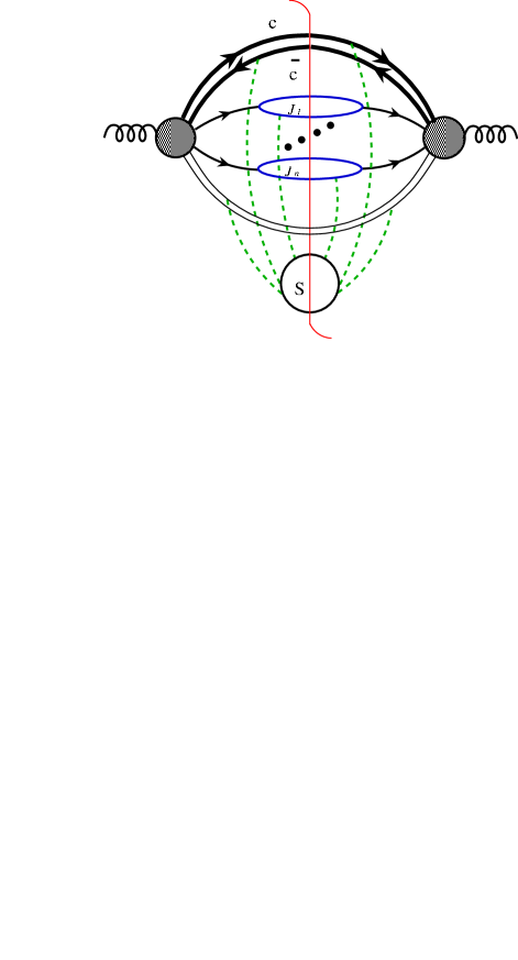
Figure 3: Physical pictures for heavy quarkonium production.

As noted in the discussion of Sec. 2.4, the physical pictures for fragmentation are similar to those for the hadronic final state interactions in leptonic annihilation. The process begins with a short-distance subdiagram, represented by a shaded circle in Fig. 3. In this case, short-distance refers to virtualities at the order of $m_{H}$. Lightlike jets, $J_{j}$, develop from energetic ($E\sim m_{H}$) “semihard” quarks, antiquarks or gluons, which emerge from the hard scattering. These jets may be connected by a diagram consisting entirely of soft quanta, $S$, to each other, and to the Wilson line that is part of the construction of the fragmentation function. In the case at hand, the heavy quark pair also emerges from the hard scattering, and soft quanta may connect to the jets and/or the Wilson line. To prove NRQCD factorization, Eq. (3), it will be necessary to show that all of this long-distance behavior either cancels or matches entirely to NRQCD matrix elements.

Considered abstractly, the connection to NRQCD is made by “integrating out” degrees of freedom at the mass scale $m_{H}$ in the calculation of the fragmentation function. In practice, that is in perturbation theory, the NRQCD operators ${\mathcal{O}}_{n}$ can be identified once we consistently separate long and short distance contributions. As the figure shows, a generic pinch surface in phase space involves not only a truly short distance part, but also a variety of semi-hard jets. The question we must ask is to what extent hadronization is affected by the presence of these jets. In the original discussion of NRQCD factorization given in Ref. [7], it was argued that in the inclusive sum over cuts in $H$ production, all infrared divergences due to soft exchanges between the heavy quarks and the extra jets cancel in the inclusive sum, even while we fix the final state of the quark pair to be a gauge singlet. Notice that even in the absence of semi-hard gluons, soft gluons may be exchanged with the Wilson line that is part of the definition of the fragmentation function. Indeed, this Wilson line is what remains of all exchanges of soft gluons between the heavy quarks and partons at relative momenta greater than $m_{H}$.

In the absence of the soft gluon connections between the heavy quarks and semi-hard gluons, the remaining physical pictures can be represented as in Fig. 4. In this case, all collinear and soft divergences associated with the jets, whose final states are summed over inclusively, cancel, just as in leptonic annihilation. Soft singularities may, and in general do, remain in the transition of the heavy quarks from short distances to hadronization, but such soft divergences are said to be “topologically factorized” [42], and are readily factorized from the hard scattering function by a standard expansion in relative velocity, as we now sketch.

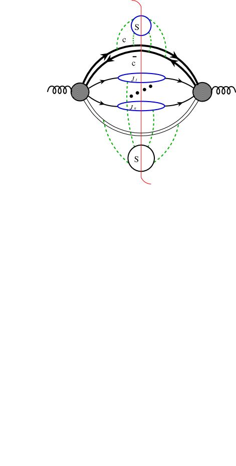
Figure 4: Topologically factored physical pictures for heavy quarkonium production.

In a topologically factorized diagram like Fig. 4, we can expand the short-distance function around vanishing relative momentum, or equivalently relative velocity $v$ of the heavy quarks. Similarly, we may decompose each diagram according to the color state (singlet or octet) of the heavy quark pair, and may also expand in the momenta of any light quanta (gluons or quark pairs) that also emerge from the short distance subdiagram. This leads precisely to an expansion in terms of local operators, creating heavy quark pairs in states $n$, labelled $c\bar{c}[n]$, where in general $[n]$ also labels the term in the expansion in relative velocity and light parton quanta, so that the corresponding operator, $\psi^{\dagger}(0){\mathcal{\kappa}}^{\prime}_{n}\chi(0)$, which always includes a quark pair, may also create light quanta. Each such operator will be accompanied by the sum of all hard subdiagrams, evaluated at zero relative velocity and at zero light parton momentum. We will refer to this sum as the hard scattering, or coefficient, function for operator $\psi^{\dagger}(0){\mathcal{\kappa}}^{\prime}_{n}\chi(0)$.

Combining the expansions from the amplitude and its complex conjugate, we derive Eq. (3), with operators that describe the creation of a heavy quark pair from the vacuum, summing over all final states that include hadron $H$. The general form of these operators [7] is

$${\mathcal{O}}^{H}_{n}(0) = \sum_{N}\ \chi^{\dagger}(0){\mathcal{\kappa}}_{n}\psi(0)\,\left|N,H\right\rangle\,\left\langle N,H\right|\,\psi^{\dagger}(0){\mathcal{\kappa}}^{\prime}_{n}\chi(0)$$ (21)

$$= \chi^{\dagger}(0){\mathcal{\kappa}}_{n}\psi(0)\,\left(a^{\dagger}_{H}a_{H}\right)\,\psi^{\dagger}(0){\mathcal{\kappa}}^{\prime}_{n}\chi(0)\,,$$

where the insertion of the creation operator $a^{\dagger}_{H}$, which is understood to act on out states to produce hadron $H$, and its conjugate enable us to sum over the complete set of out states between the creation and annihilation operators. The first form defines the sum over final states appropriate to quarkonium production, while the second form is a convenient shorthand.

The following discussion is an attempt to analyze the basic assumption that enables us to expand in $v$ in this manner. That is, we will begin with the general momentum region illustrated by Fig. 3 and explore the reduction to the simpler “topologically factorized” picture of Fig. 4, by testing the cancellation of soft exchanges between the heavy quarks and semi-hard gluons, or equivalently, the Wilson line.

3.3 Operators and gauge completion

Our first observation, already described in [17], is that matrix elements of the form (21) are not invariant under operator-valued gauge transformations. In general, the onium creation operators $a_{H}$ and $a^{\dagger}_{H}$, which act on out states, need not commute with gauge transformations carried out at the origin, even though they are themselves color singlets. As a result, it seems most natural to us to modify the operators (21) to provide a form precisely analogous to the gauge-invariant definitions of fragmentation functions in Eq. (15) above,

$${\mathcal{O}}^{H}_{n}(0)\to\chi^{\dagger}(0){\mathcal{\kappa}}_{n,c}\psi(0)\,\Phi_{l}^{(A)}{}^{\dagger}(0){}_{cb}\,\left(a^{\dagger}_{H}a_{H}\right)\,\Phi_{l}^{(A)}(0)_{ba}\,\chi^{\dagger}(0){\mathcal{\kappa}}^{\prime}_{n,a}\psi(0)\,,$$ (22)

in terms of ordered exponentials, defined as in Eq. (14). In the (complex conjugate) amplitudes, (anti)time-ordering is understood. We emphasize that such a redefinition is not required for self-consistency. If one can demonstrate NRQCD factorization in terms of operators in any specific gauge, a gauge-dependent definition of the operator matrix elements is admissible, as long as the gauge-dependence is not infrared sensitive. Indeed, this is the case for fragmentation functions, because of the cancellation of infrared divergences in final-state interactions at high $P_{T}$, as observed above. In the absence of a similar demonstration of infrared finiteness for the refactorization (3) of fragmentation functions in terms of NRQCD operators, however, it seems natural to entertain (22) as a plausible replacement. We now turn to the expansion in relative velocity, which will enable us to test our suggestion.

4 Velocity expansion

4.1 Requirements for NRQCD factorization

To study the role of soft gluon emission in heavy quarkonium production, we will analyze infrared divergences in the production amplitude for two heavy quarks, of total momentum $P$ and relative momentum, $q$:

$$P_{1}=\frac{P}{2}+q\equiv p+q\qquad P_{2}=\frac{P}{2}-q\equiv p-q\,.$$ (23)

That is, we study the process $g\to c\bar{c}[{n_{0}}]+X$ with $c\bar{c}[{n_{0}}]=c(p+q)\bar{c}(p-q)$. The lowest-order diagram for this fragmentation function is shown in Fig. 5. It consists of a single gluon splitting into the quark-anti-quark pair.

Figure 5: Lowest-order fragmentation function for $g\to c\bar{c}$. There are no interactions on the eikonal quark pair or the Wilson line that corresponds to an eikonal gluon of four-velocity $l$.

In the following, we will study infrared divergences in soft gluon corrections to this process, when the quark-antiquark pair is created as a color octet, but is restricted to a singlet in the final state. Otherwise, we sum over all perturbative final states.

To form a heavy quarkonium, of course, these quarks cannot be truly on-shell. Rather, they are off-shell by an energy of order $q^{2}/m_{c}$, characteristic of a Coulomb bound state [41]. These are nonperturbative effects, however, while coefficient functions are calculated in perturbation theory. The cancellation of divergences, and/or their matching to matrix elements in soft-gluon corrections to Fig. 5 is a necessary condition for NRQCD factorization. Any remaining divergences would be a violation of factorization. In our calculation below, we will find uncanceled divergences at NNLO for conventional operators, which, however, may be absorbed into gauge-completed NRQCD operators.

4.2 Expansion in the eikonal approximation

Because our calculation will be carried out with on-shell quarks, we can use the eikonal approximation for the coupling of soft gluons to the quarks in order to identify infrared divergences in the cross section. Equivalently, we may treat the quarks in heavy-quark effective theory to leading order in their mass. Yet another equivalent, and for us particularly convenient, approach is to replace the quarks by path-ordered exponentials, similar to Eq. (14) above, but now with time-like velocities representing the quark and antiquark.

The dimensions of the velocity in ordered exponential (14) can be shifted by a change of variables in the parameter $\lambda$. For this reason, we are free to identify the quark velocities directly with their momenta $P_{1,2}=(P/2\pm q)$. At fixed (and unequal) values of $P_{1}$ and $P_{2}$, all infrared divergences can be found by the eikonal approximation. The eikonal approximation and hence infrared divergences are completely independent of any spin projections that we may make on the state of the quark pair. As a result, soft gluon emission separates from all dynamical factors that involve the spins of the quarks, and enters as a multiplicative factor. We will come back to the limit $P_{1}=P_{2}$ below.

We can classify the eikonal infrared-sensitive factors by the color of the $c\bar{c}$ pair at creation (the origin of the ordered exponentials) and by their color in the final state. Gluon emission, of course, will mix these states. For an NRQCD-like factorization to hold, if we fix the color of the $c\bar{c}$ pair in the final state, infrared divergences either cancel or can be matched with matrix elements [7]. Finite remainders will be associated with coefficient functions, as in the NLO calculations of Refs. [35]-[40]

In summary, we will study the infrared factor associated with the creation of a $c\bar{c}$ pair in an octet configuration, and its evolution into a singlet in the final state. This infrared factor may be written in the notation of Eq. (14) as

$${\cal I}^{(8\to 1)}(P_{1},P_{2}) = \sum_{N}<0|\,\left[\Phi_{P_{2}}^{(\bar{q})}{}^{\dagger}(0)\right]_{IJ}\left[T_{d}\right]_{JK}\ \left[\Phi_{P_{1}}^{(q)}{}^{\dagger}(0)\right]_{KI}\,\Phi_{l}^{(A)}{}^{\dagger}(0)_{db}\,\left|N\right\rangle$$ (24)

$$\hskip 56.9055pt\times\left<N\right|\Phi_{l}^{(A)}(0)_{bc}\,\left[\Phi_{P_{1}}^{(q)}(0)\right]_{LM}\left[T_{c}\right]_{MN}\left[\Phi_{P_{2}}^{(\bar{q})}(0)\right]_{NL}\,|0\rangle\,,$$

where we have exhibited all color indices: those in adjoint representation by $a,\,b\dots$, and those in the fundamental representation by $I,\,J\dots$, to indicate the trace structure, which imposes a color singlet configuration in the final state.

The operator $\Phi^{(\bar{q})}$ is the ordered exponential that represents the antiquark. It has the opposite sign on the coupling compared to the quark operator, and has color matrices ordered in the reverse sense to time ordering. In the notation of the standard definition, Eq. (14), we represent this matrix ordering by $\bar{\cal P}$, and define

$$\Phi_{P_{2}}^{(\bar{q})}(0)=\bar{\cal P}\exp\left[ig\int_{0}^{\infty}d\lambda\,P_{2}\cdot A^{(q)}(P_{2}\lambda)\right]\,.$$ (25)

Here $A^{(q)}_{\nu}\equiv\sum_{a}T_{a}\,A_{\nu,\,a}$ is the matrix-valued field in the quark fundamental representation. For classical fields, $\Phi_{n}^{(\bar{q})}(0)$ is the hermitian conjugate of $\Phi_{n}^{(q)}(0)$. In Eq. (24) and below, overall time-ordering of the field operators is understood in the amplitude, and anti-time ordering in its complex conjugate. For explicit computations, we restrict the sum over final states $N$ in Eq. (24) to soft gluon emission only.

The graphical rules for the interactions of gluons with the ordered exponentials are exactly the same as the eikonal approximation, and propagators and vertices are given by

$$\frac{i}{(\beta\cdot k+i\epsilon)}\quad,\quad\pm ig_{s}T_{a}\beta^{\mu}\,,$$ (26)

with the plus for antiquarks and the minus for quarks on the vertex and with $\beta^{\mu}$ the time-like quark four-velocity. The quark and antiquark eikonal propagators are represented as heavy lines on the left-hand side of Fig. 6. In this notation, Eq. (24) describes a product of color traces in the fundamental representation. Our ability to use the same notation for velocities as for momenta is manifest since the combination of each eikonal vertex and propagator is scale-invariant. In the pair rest frame the relative velocity of the members of the pair is proportional to the ratio $q^{2}/m_{c}^{2}=4q^{2}/P^{2}$.

In the spirit of NRQCD analysis, and because it leads to some simplification, we will study corrections to Fig. 5 to order $q^{2}$, which is the first nontrivial order. At zeroth order in $q^{2}$, the quark and antiquark never separate, and all infrared divergences cancel, since there are no color multipoles to which they can couple. We can see this in Eq. (24), in which both the amplitude and complex conjugate amplitude reduce to unity in the limit $P_{1}=P_{2}\to P/2$. This is easily proved by considering the $A(x)$-field with the largest time in the amplitude. This field may come either from the quark exponential, $\Phi_{P_{1}}^{(q)}(0)$, or the antiquark exponential $\Phi_{P_{2}}^{(\bar{q})}(0)$. When $P_{1}=P_{2}$, the only difference between these two terms is the relative minus sign between the quark and antiquark vertices. Every such pair of terms cancels pairwise. An identical argument applies to the complex conjugate amplitude, and there is therefore no overall $q$ term, and $q^{2}$ can be reached only by expanding both the amplitude and its complex conjugate to order $q$ independently.

The expansion to order $q$ is straightforward, and has a nice interpretation in terms of fields. We start with the expansion for the individual ordered exponentials,

$$q^{\nu}\frac{\partial}{\partial p^{\nu}}\ \Phi_{p}^{(q)}(0) =-ig\int_{0}^{\infty}d\lambda^{\prime}\,\lambda^{\prime}\,{\cal P}\exp\left[-ig\int_{\lambda^{\prime}}^{\infty}d\lambda\;p\cdot A^{(q)}(\lambda p)\right]$$

$$\hskip 56.9055pt\times\;\left[\,p^{\mu}q^{\nu}F_{\nu\mu,a}(\lambda^{\prime}p)T_{a}\,\right]\;{\cal P}\exp\left[-ig\int_{0}^{\lambda^{\prime}}d\lambda\;p\cdot A^{(q)}(\lambda p)\right]$$

$$-q^{\nu}\frac{\partial}{\partial p^{\nu}}\ \Phi_{p}^{({\bar{q}})}(0) =-ig\int_{0}^{\infty}d\lambda^{\prime}\,\lambda^{\prime}\,T\,\Bigg{\{}\,\bar{\cal P}\exp\left[ig\int_{0}^{\lambda^{\prime}}d\lambda\;p\cdot A^{(q)}(\lambda p)\right]$$ (27)

$$\hskip 56.9055pt\times\;\left[\,p^{\mu}q^{\nu}F_{\nu\mu,a}(\lambda^{\prime}p)T_{a}\,\right]\;\bar{\cal P}\exp\left[ig\int_{\lambda^{\prime}}^{\infty}d\lambda\;p\cdot A^{(q)}(\lambda p)\right]\Bigg{\}}\,,$$

where the explicit minus sign on the left in the second expression anticipates that we will be expanding in the momentum of the anti-quark, $P_{2}=p-q$. In both of these expressions, the time-ordering is from right (earlier) to left (later), with an (opposite) identical ordering of color matrices for the (anti) quark exponential. We have inserted an explicit $T$ in the antiquark expression, to remind ourselves that the operators and color matrices have the opposite ordering in this case. The operator $F_{\mu\nu,a}$ is the gluon field strength with tensor and color indices. Note the overall factor of $\lambda^{\prime}$, which reflects the increasing separation of the quark and antiquark paths with increasing distance from the origin when $q$ is changed by a constant amount.

Figure 6: Velocity expansion. The heavy solid lines represent heavy quark propagators in the eikonal approximation.

We now apply Eq. (27) to the amplitudes in Eq. (24). Expanding $P_{1}$ and $P_{2}$ about $p\equiv P/2$ we find

$$q^{\nu}\frac{\partial}{\partial q^{\nu}}\ \left<N\right|\Phi_{l}^{(A)}(0)_{bc}\,\left[\Phi_{P_{1}}^{(q)}(0)\right]_{LM}\left[T_{c}\right]_{MN}\left[\Phi_{P_{2}}^{(\bar{q})}(0)\right]_{NL}\ \,|0\rangle\bigg{|}_{q=0} =$$ (28)

$$-ig\left<N\right|\,\Phi_{l}^{(A)}(0)_{bc}\,\left[{\cal P}\exp\left[-ig\int_{0}^{\infty}d\lambda\,p\cdot A^{({q})}(\lambda p)\right]\,\right]_{LM}\left[T_{c}\right]_{MN}$$

$$\times\,\int_{0}^{\infty}d\lambda^{\prime}\,\lambda^{\prime}\,\Bigg{\{}\,\bar{\cal P}\exp\left[ig\int_{0}^{\lambda^{\prime}}d\lambda\;p\cdot A^{(q)}(\lambda p)\right]$$

$$\times\;\left[\,p^{\mu}q^{\nu}F_{\nu\mu,a}(\lambda^{\prime}p)T_{a}\,\right]\;\bar{\cal P}\exp\left[ig\int_{\lambda^{\prime}}^{\infty}d\lambda\;p\cdot A^{(q)}(\lambda p)\right]\Bigg{\}}_{NL}\,\,|0\rangle$$

$$-ig\left<N\right|\,\Phi_{l}^{(A)}(0)_{bc}\,\int_{0}^{\infty}d\lambda^{\prime}\,\lambda^{\prime}\,\Bigg{\{}{\cal P}\exp\ \left[-ig\int_{\lambda^{\prime}}^{\infty}d\lambda\,p\cdot A^{(q)}(\lambda p)\right]$$

$$\times\;\left[\,p^{\mu}q^{\nu}F_{\nu\mu,a}(\lambda^{\prime}p)T_{a}\,\right]\;{\cal P}\exp\left[-ig\int_{0}^{\lambda^{\prime}}d\lambda\,p\cdot A^{(q)}(\lambda p)\right]\Bigg{\}}_{LM}\left[T_{c}\right]_{MN}$$

$$\times\left[\bar{\cal P}\exp\left[ig\int_{0}^{\infty}d\lambda\,p\cdot A^{(q)}(\lambda p)\right]\,\right]_{NL}\,|0\rangle\,.$$

Here again, time ordering is understood for all field operators. The lowest order of the expansions of the left- and right-hand sides of Eq. (28) are shown graphically in Fig. 6. On the right, the vertex associated with the field strength in the final form is represented by $\otimes$.

We next apply reasoning similar to that which led to the cancellation of the ordered exponentials at $q=0$. Again, consider the $A$-field with largest variable $\lambda$, assuming that there is at least one such field with $\lambda>\lambda^{\prime}$, that is, at least one field at a larger time than the field strength $p^{\mu}q^{\nu}F_{\nu\mu}$. We recognize that whenever we find such a field, there is a cancellation between the cases when that field is associated with the quark and antiquark ordered exponentials. All fields at times greater than that of the field strength cancel, and we have

$$q^{\nu}\frac{\partial}{\partial q^{\nu}}\ \left<N\right|\Phi_{l}^{(A)}(0)_{bc}\,\left[\Phi_{P_{1}}^{(q)}(0)\right]_{LM}\left[T_{c}\right]_{MN}\left[\Phi_{P_{2}}^{(\bar{q})}(0)\right]_{NL}\ \,|0\rangle\bigg{|}_{q=0} =$$

$$-ig\left<N\right|\,\Phi_{l}^{(A)}(0)_{bc}\,\int_{0}^{\infty}d\lambda^{\prime}\,\lambda^{\prime}\,\left[{\cal P}\exp\left[-ig\int_{0}^{\lambda^{\prime}}d\lambda\,p\cdot A^{({q})}(\lambda p)\right]\,\right]_{LM}\left[T_{c}\right]_{MN}$$

$$\times\,\Bigg{\{}\,\bar{\cal P}\exp\left[ig\int_{0}^{\lambda^{\prime}}d\lambda\;p\cdot A^{(q)}(\lambda p)\right]\;\left[\,p^{\mu}q^{\nu}F_{\nu\mu,a}(\lambda^{\prime}p)T_{a}\,\right]\;\Bigg{\}}_{NL}\,\,|0\rangle$$

$$-ig\left<N\right|\,\Phi_{l}^{(A)}(0)_{bc}\,\int_{0}^{\infty}d\lambda^{\prime}\,\lambda^{\prime}\,\Bigg{\{}\;\left[\,p^{\mu}q^{\nu}F_{\nu\mu,a}(\lambda^{\prime}p)T_{a}\,\right]\;{\cal P}\exp\left[-ig\int_{0}^{\lambda^{\prime}}d\lambda\,p\cdot A^{(q)}(\lambda p)\right]\Bigg{\}}_{LM}\left[T_{c}\right]_{MN}$$

$$\times\left[\bar{\cal P}\exp\left[ig\int_{0}^{\lambda^{\prime}}d\lambda\,p\cdot A^{(q)}(\lambda p)\right]\,\right]_{NL}\,|0\rangle$$

$$\hskip 14.22636pt=-2ig\left<N\right|\,\Phi_{l}^{(A)}(0)_{bc}\,\int_{0}^{\infty}d\lambda^{\prime}\,\lambda^{\prime}\,{\rm Tr}\,\Bigg{\{}\;\left[\,p^{\mu}q^{\nu}F_{\nu\mu,a}(\lambda^{\prime}p)T_{a}\,\right]$$

$$\hskip 28.45274pt\times\;{\cal P}\exp\left[-ig\int_{0}^{\lambda^{\prime}}d\lambda\,p\cdot A^{(q)}(\lambda p)\right]\;T_{c}\;\bar{\cal P}\exp\left[ig\int_{0}^{\lambda^{\prime}}d\lambda\,p\cdot A^{(q)}(\lambda p)\right]\,\Bigg{\}}\,|0\rangle\,.$$ (29)

In the last line we have used the cyclic nature of the color trace and the anti-path ordering of the antiquark exponential to show that the two terms above are equal. Next, we note that were it not for the generator $T_{c}$, we could use the same reasoning as above to show that the $A$-field of lowest $\lambda^{\prime}$ cancels between the quark and antiquark exponentials. The nonvanishing remainder, therefore, is a commutator,

$$-igA_{d}\left(\lambda_{\mathrm{m}in}p\right)\left[\,T_{d},T_{c}\,\right] = gA_{d}\left(\lambda_{\mathrm{m}in}p\right)\,f_{dce}T_{e}$$ (30)

$$= -igA_{d}\left(\lambda_{\mathrm{m}in}p\right)\,[T_{d}^{(A)}]_{ec}\,T_{e}\,,$$

$$= T_{e}\,\left(-igA^{(A)}\left(\lambda_{\mathrm{m}in}p\right)\,\right)_{ec}\,,$$

where $[T^{(A)}_{d}]_{ec}=-if_{dec}$ is a generator in the adjoint representation. In effect, the gluon field is converted from the fundamental representation to the adjoint.

At any order in $g$, this procedure may be repeated until all $A$-fields from the remaining ordered exponentials have been converted from fundamental to adjoint representation in Eq. (29). The final color trace in fundamental representation is trivial (and gives $1/2$), and we derive the relatively simple form

$$q^{\nu}\frac{\partial}{\partial q^{\nu}}\ \left<N\right|\Phi_{l}^{(A)}(0)_{bc}\,\left[\Phi_{P_{1}}^{(q)}(0)\right]_{LM}\left[T_{c}\right]_{MN}\left[\Phi_{P_{2}}^{(\bar{q})}(0)\right]_{NL}\,|0\rangle\Bigg{|}_{q=0} =$$ (31)

$$-ig\int_{0}^{\infty}d\lambda^{\prime}\,\lambda^{\prime}\,\left<N\right|\,\Phi_{l}^{(A)}(0)_{bc}\,\left[\,p^{\mu}q^{\nu}F_{\nu\mu,a}(\lambda^{\prime}p)\,\right]\Bigg{\{}\;{\cal P}\exp\left[-ig\int_{0}^{\lambda^{\prime}}d\lambda\,p\cdot A^{(A)}(\lambda\,p)\right]\Bigg{\}}_{ac}\,\,|0\rangle$$

$$=-ig\int_{0}^{\infty}d\lambda^{\prime}\,\lambda^{\prime}\,\left<N\right|\,\Phi_{l}^{(A)}(0)_{bc}\,\left[\,p^{\mu}q^{\nu}F_{\nu\mu,a}(\lambda^{\prime}p)\,\right]\Phi_{p}^{(A)}(\lambda^{\prime})_{ac}\,\,|0\rangle\,,$$

in which all fields are in adjoint representation. There is only a single ordered exponential, linking the gauge index at the origin ($c$) with the field strength at the variable point $\lambda^{\prime}$. Note that the index $c$ of $\Phi_{p}^{(A)}$ is itself linked to the final state by the auxiliary ordered exponential that we have added in the $l$ direction through gauge completion, as described above and in Ref. [17].

To derive contributions of order $v^{2}$, or equivalently $q^{2}/m_{c}^{2}=4q^{2}/P^{2}$, we will study the nonlocal matrix element

$${\cal I}_{2}(p,q) \equiv$$ (32)

$$\sum_{N}\int_{0}^{\infty}d\lambda^{\prime}\,\lambda^{\prime}\,\left<0\right|\,\Phi_{l}^{(A)}{}^{\dagger}(0)_{bc^{\prime}}\,\Phi_{p}^{(A)}(\lambda^{\prime}){}^{\dagger}_{a^{\prime}c^{\prime}}\,\left[\,p^{\mu}q^{\nu}F_{\nu\mu,a^{\prime}}(\lambda^{\prime}p)\,\right]\,\left|N\right\rangle$$

$$\times\left\langle N\right|\int_{0}^{\infty}d\lambda^{\prime}\,\lambda^{\prime}\,\Phi_{l}^{(A)}(0)_{bc}\,\left[\,p^{\mu}q^{\nu}F_{\nu\mu,a}(\lambda^{\prime}p)\,\right]\Phi_{p}^{(A)}(\lambda^{\prime})_{ac}\,\,|0\rangle\,.$$

As above, (anti-) time ordering is implicit in the (complex conjugate) amplitudes. This is the complete ${\cal O}(v^{2})$ result for ${\cal I}^{(8\to 1)}$, Eq. (24), because, as we have seen above, at order ${\cal O}(v^{0})$, the quark and anitquark eikonal lines in both the amplitude or its complex conjugate cancel completely, and thus decouple for soft radiation.

In the following, we will study the expansion of Eq. (32) to NNLO. The explicit factor of $\lambda^{\prime}$ in Eq. (31) modifies the eikonal propagators. To see this, we can formally evaluate the $\lambda^{\prime}$ integral in Eq. (31) in terms of the Fourier transform of the field strength, $\tilde{F}_{\nu\mu,a}(k)\equiv\int d^{4}xF_{\nu\mu,a}(x)\exp[-ik\cdot x]$. With this convention, momentum $k$ flows into the field strength (and hence out of the eikonal lines). For a given order in the expansion of the adjoint ordered exponential in Eq. (31), the lower limit of the $\lambda^{\prime}$ integral is some value $\lambda_{m}$, the maximum value of $\lambda$ in the ordered fields $p\cdot A^{(A)}(\lambda p)$ from $\Phi_{p}^{(A)}$. The relevant integral is then

$$-ig\int_{\lambda_{m}}^{\infty}d\lambda^{\prime}\,\lambda^{\prime}\int{d^{4}k\over(2\pi)^{4}}\,{\rm e}^{i\lambda^{\prime}(n\cdot k+i\epsilon)}\,\tilde{F}_{\nu\mu,a}(k) =$$ (33)

$$-ig\int{d^{4}k\over(2\pi)^{4}}\,{\rm e}^{i\lambda_{m}(n\cdot k+i\epsilon)}\,\tilde{F}_{\nu\mu,a}(k)\,\left[\,\lambda_{m}\,\frac{i}{n\cdot k+i\epsilon}-\frac{1}{(n\cdot k+i\epsilon)^{2}}\,\right]\,,$$

where we have integrated by parts. The second term gives a squared eikonal propagator. The first (boundary) term in brackets on the right-hand side gives the standard eikonal propagator of Eq. (26), times a factor of $\lambda_{m}$, producing a similar pattern in the next integral. The next integral will again give a squared propagator plus a boundary term, until the final $\lambda$ integral, for which the lower limit is zero and the boundary term vanishes. The result for a specific diagram is to replace the standard product of eikonal propagators by a sum of terms, in each of which one of the propagators is squared. Vertices for the operators $p\cdot A$ are unchanged. The relevant graphical notations for vertices are shown in Fig. 7. The three-point field strength vertex may be represented as

$$U^{\mu}_{F,ac}(p,q,k)=-g\,\delta_{ac}\,\left((p\cdot k)q^{\mu}-(q\cdot k)p^{\mu}\right)\,,$$ (34)

and the four-point vertex as

$$W^{\mu\nu}_{F,abc}(p,q)=ig^{2}f_{abc}\,\left(\,p^{\mu}q^{\nu}-q^{\mu}p^{\nu}\,\right)\,.$$ (35)

In both cases, $c$ represents the color factor of the field strength tensor of Eq. (31), while $a$ and/or $b$ are the color indices of the gluon(s) that couple to the field strength. Because the adjoint eikonal lines end at the field strength in (31), corresponding to the color singlet pair in the final state, the three- and four-point vertices have only two and three color indices, respectively.

(a)                                (b)                                (c)                                (d)

Figure 7: a) Eikonal vertex; (b,c) vertices for the field strength; (d) line with eikonal and field strength interactions.

As an example, corresponding to Fig. 7d, we have the expression

$$g\,P^{\mu^{\prime}}\ U^{\mu}_{F,ac}(P,q,k)\;\left[\;\frac{1}{-P\cdot k^{\prime}+i\epsilon}\,\frac{1}{(-P\cdot k+i\epsilon)^{2}}+\frac{1}{(-P\cdot k^{\prime}+i\epsilon)^{2}}\,\frac{1}{-P\cdot k+i\epsilon}\;\right]\,,$$ (36)

where we have chosen the sign of the infinitesimal imaginary part appropriate to the amplitude. To avoid clutter in and proliferation of figures, we will not introduce a graphical notation for squared propagators, but simply assume that the sum over terms is carried out in every diagram with a field strength operator at the largest time.

The three-point vertex, $U^{\mu}_{F}$ in Eq. (34) is just the momentum representation of the Maxwell term of the field strength. It thus trivially decouples from scalar-polarized gluons,

$$U^{\nu}_{F}(p,q,k)k_{\nu}=0\,.$$ (37)

This result will lead to considerable simplification in our calculations; in particular, it eliminates, on a diagram-by-diagram basis, collinear poles associated with the octet eikonal line in the $\ell$ direction. This is because in any covariant gauge, collinear divergences are associated with gluons whose polarization is proportional to their momenta in the collinear limit [20].

In the next two sections, we apply these rules to study the coupling of soft gluons to the heavy quark pair. We begin at NLO, and then generalize to NNLO.

5 Next-to-leading Order

Figs. 8a and b illustrate the origin of infrared divergences in the fragmentation function at next-to-leading order in $\alpha_{s}$ to order $v^{2}$. This infrared structure is the same as the lowest order contribution to ${\cal I}_{2}$, Eq. (32). As in Fig. 6, the sum over gluon connections to quark and antiquark on each side of the cut has been replaced by a single field-strength vertex. Because the parent gluon is off-shell by order $m_{c}$, we may contract it to a point to study soft gluon corrections. For this purpose, it is then equivalent to study the matrix elements (24) to next-to-leading order, and that is how we shall describe our calculation below. We emphasize, however, that there is a trivial mapping from the matrix elements to the fragmentation functions.

The vertical lines in Fig. 8 represent the quark-antiquark pair in the final state, and a projection onto a color singlet (implemented by a color trace) is understood, along with a sum over all connections of the gluon to the quark and antiquark. The full set of diagrams is found by completing the cut, which can be done in only one way for 8a, where the gluon must be in the final state. For Fig. 8b, on the other hand, there are two possibilities, one with a virtual gluon correction and one with a real gluon. In fact, of the two diagrams, only 8a can contribute to ${\cal I}^{(8\to 1)}$, Eq. (24). If we require a color singlet pair in the final state Fig. 8b requires interference between octet and singlet in the hard scattering functions. We consider this diagram because it follows a pattern observed in the original arguments for NRQCD factorization, given in Ref. [7], and because its square contributes to ${\cal I}^{(8\to 1)}$ at NNLO.

(a)                                            (b)

Figure 8: Representative NLO contributions to $g\to c\bar{c}$ fragmentation in eikonal approximation are found by all cuts of these diagrams. In these figures, the parent gluon is contracted to a point, represented by the dark circle, because it is off-shell by order $m_{c}$. .

Let us begin with Fig. 8a, which has a topologically-factorized form, in which the soft gluon connects only to the heavy quarks, rather than to other finite-energy final-state lines. (In this case, the only such line is the eikonal line in direction $l$.) From the perturbative rules described above, we immediately write down the following integral, which is readily evaluated in $D=4-2\varepsilon$ dimensions,

$$\Sigma^{(8a)}(P,q)~{} = ~{}16\,g^{2}\mu^{2\varepsilon}\,\int\frac{d^{D}k}{(2\pi)^{D-1}}~{}\delta(k^{2})\,[q_{\nu}(P\cdot k)-(q\cdot k)P_{\nu}]$$ (38)

$$\hskip 85.35826pt\times\ [q^{\nu}(P\cdot k)-(q\cdot k)P^{\nu}]\frac{1}{[(P\cdot k)^{2}]^{2}}$$

$$= {16\over 3}\,{\alpha_{s}\over\pi}\,{\vec{q}\,{}^{2}\over P^{2}}\,{1\over-\varepsilon}+\dots\,.$$

Here we have suppressed color factors, including the factor of 1/2 from the color trace mentioned above Eq. (31). The infrared pole in this result is familiar from NLO calculations of fragmentation [35, 36, 37], in which it is matched to the relevant NRQCD matrix element.

We now turn to the cuts of Fig. 8b, which contribute only to color interference terms. These diagrams, in which the gluon connects the quark-antiquark pair with the eikonal line, are not topologically factorized. Based on the arguments of [7], we expect these to cancel, and they do. This was verified explicitly in Ref. [38] for the case of color octet pairs in the final state. It will be instructive, however, to see how this happens in our velocity-expanded form to linear order in $q$ with a color singlet final state, because the cancelation found here will be relevant to NNLO.

We consider first the cut diagram with a virtual gluon loop in the amplitude. For our purposes, the overall normalization of the diagram is arbitrary, and we write

$$\Sigma^{(8b)}_{\rm virtual}=g^{2}\int\frac{d^{D}k}{(2\pi)^{D}}\,N(P,k,q,\ell)\,{1\over(P\cdot k+i\epsilon)^{2}}\;{1\over k^{2}+i\epsilon}\ {1\over-\ell\cdot k+i\epsilon}\,,$$ (39)

with numerator factor

$$N(P,k,q,\ell) = 2\,\left[q\cdot\ell\,(P\cdot k)-P\cdot\ell\,(q\cdot k)\right]$$ (40)

$$= \sqrt{2}\;P_{0}\;\ell^{-}\,\left[\sqrt{2}k^{+}q_{3}+q_{\perp}\cdot k_{\perp}\right]\,.$$

In this diagram, as in subsequent loop integrals, we will integrate first the minus loop momentum, by closing contours in the lower half-plane and picking up the relevant poles. Certain regularities and cancellations are conveniently represented in this manner, reducing the number of diagrams that must be computed explicitly. The result is shown in Fig.  9.

(a)                                   (b)                                   (c)

Figure 9: a,b) Poles resulting from closing the minus loop integral in cut diagrams corresponding to Fig. 8b. c) Corresponding representation of real gluon emission.

The double pole from the quark pair octet eikonal denominator, $(P\cdot k+i\epsilon)^{2}$, is always in the $k^{-}$ lower half-plane, while the pole of the exchanged gluon is in the lower half-plane only when $k^{+}$ flows in the direction indicated in the figure. Closing in the lower half-plane, and neglecting the term odd in $k_{\perp}$ we find only a terms proportional to $q_{3}$,

$$\Sigma^{(8b)}_{\rm virtual,1} = i\,4\,\frac{q_{3}}{P_{0}}\ \frac{g^{2}}{(2\pi)^{D-1}}\,\int d^{D-2}k_{\perp}\int_{-\infty}^{\infty}dk^{+}\;\Bigg{\{}\,{d\over dk^{-}}\left({1\over k^{2}+i\epsilon}\right)\Bigg{|}_{k^{-}=-k^{+}}$$

$$\hskip 156.49014pt+\theta(k^{+})\,\frac{1}{2k^{+}}\,{1\over(k^{+}{}+k_{\perp}^{2}/2k^{+})^{2}}\,\Bigg{\}}$$

$$=i\,4\,\frac{q_{3}}{P_{0}}\frac{g^{2}}{(2\pi)^{D-1}}\,\int d^{D-2}k_{\perp}\left\{\int_{-\infty}^{\infty}dk^{+}\;{-2k^{+}\over(2k^{+}{}^{2}+k_{\perp}^{2})^{2}}\;+\int_{0}^{\infty}{dk^{+}\over 2k^{+}}{1\over(k^{+}+k_{\perp}^{2}/2k^{+})^{2}}\,\right\}\,.$$

These two terms correspond to the diagrams in Fig. 9a and b, where the straight line through the eikonal or gluon line indicates the $k^{-}$ pole chosen. Both of these terms are logarithmically divergent by power-counting in the soft limit. As in the case above, however, they are collinear finite. In fact, the first term on the right-hand side is odd in $k^{+}$ and vanishes after symmetric integration. The pole at $k^{+}=0$, which would correspond to an on-shell intermediate state, has vanishing residue at order $q$.

In the second term of the right-hand side of Eq. (LABEL:nlopoleterms), the exchanged gluon is on-shell with positive plus momentum flowing from the heavy quark pair to the eikonal lines. Its contribution to the cross section, as illustrated in Fig. 9b, is real, and it is straightforward to verify that it cancels the corresponding diagram for real gluon emission, illustrated by Fig. 9c, which has a standard flow of gluon momentum ($k^{+}>0$) in the cut diagram. We will use the notation shown in these figures to help organize our NNLO computations below.

At the level of NLO, we have found that one-loop corrections indeed follow the expected pattern: they cancel except when topologically-factorized, and are thus consistent with matching to conventional NRQCD matrix elements. The presence of the octet Wilson line in our gauge-completed matrix elements does not change this pattern at NLO, as observed in Ref. [38]

Before going on to the details of the NNLO calculations, we make a comment on gauge independence. As defined, the factorized fragmentation functions are gauge invariant, since the eikonal and the pair creation operators $\Phi^{(A)}_{\ell}\psi^{\dagger}{\cal K}_{n}\chi$ of Eq. (22) are contracted to form a color singlet vertex. Also, as we have seen, because of Eq. (37), there are immediate cancellations of many gauge terms like $k^{\mu}k^{\nu}/(k^{2})^{2}$ for a gluon of momentum $k$, because of the field strength vertices that appear when we expand in the relative velocity of the quark pair. We can, of course, decouple the eikonal gauge line entirely, by choosing an $\ell\cdot A=0$ gauge. The gauge invariance of the matrix elements assure that the result would be the same. For our purposes, however, Feynman gauge is most convenient.

6 The Fragmentation Function at NNLO

In this section we study in detail the infrared behavior of the gauge-completed gluon fragmentation function at NNLO. Specifically, we will study non-topologically factorized diagrams at order $\alpha_{s}^{2}$ in Eq. (24). We will find uncanceled infrared divergences for this set of diagrams, corresponding to ${\cal O}(v^{2})$ contributions to the fragmentation functions. We emphasize that the same infrared poles (proportional to $\alpha_{s}^{2}/(-\varepsilon)$) appear in cross sections, associated with soft gluon exchanges between the quark pair and a recoiling gluon. For this reason, the gauge-completion of matrix elements is necessary for factorization. At the same time, we will observe that the infrared pole is independent of the direction of the vector $\ell^{\mu}$. This shows that the gauge-completed fragmentation function is universal to NNLO. The same fragmentation function will match infrared poles for the quark pair recoiling against a gluon in any frame, or indeed (as we shall see), for any set of recoiling jets at this order of soft gluon exchange. We are not yet able to show, however, that this redefinition is universal at all orders in soft gluon exchange.

6.1 The diagrams

The soft-gluon diagrams that we will evaluate are shown in Fig. 10. Here, we compute only those contributions that correspond to the transition of a color octet pair to color singlet in both amplitude and complex conjugate. For NRQCD factorization to hold, all infrared divergences should either cancel or factorize into octet matrix elements.

We will discuss the diagrams of Fig. 10 one at a time. In evaluating each diagram, $k_{1}$ is defined as the momentum of the gluon that attaches to the quark pair at the left-most vertex, and it is always chosen to flow left to right in the diagrams. We label the momentum of the remaining gluon line attached to the quark pair as $k_{2}$, choosing it to flow upward to the pair in each case. As observed in Sec. 5, the structure of the field strength vertex automatically eliminates collinear poles associated with soft gluons parallel to the $\ell$ direction.

For the purposes of this section, momenta associated with the quark eikonal lines, $P$, $p=P/2$ and $q$, will all be scaled by the quark mass, $m_{c}$. In the quarkonium rest frame, then, we have $P=(2,\vec{0})$, $p=(1,\vec{0})$ and $q=(0,\vec{v}/2)$.

(I)                                              (II)                                              (III)

(IV)                                              (V)                                              (VI)

Figure 10: Diagrams I - VI discussed in the text. We sum over all cuts of these diagrams that can produce a color singlet quark pair. At the hard vertex, the pair is created in an octet state.

6.2 Summary of results

In the remainder of this section, we have given the calculations that confirm our claims above in substantial detail. Since this discussion is of necessity rather detailed, it may be useful to summarize our results at the outset. Each of the diagrams in Fig. 10 contributes to the NNLO infrared factor in three separate quantities: first, the inclusive cross section for the production of a color-singlet charm pair of total momentum $P$ to order $q^{2}$ in their relative momentum, through the fragmentation of an off-shell gluon; second, the fragmentation function for a gluon to the same color-singlet pair; and third, the gauge-completed production matrix element Eq. (22) for the production of the color-singlet pair from a local color-octet combination of quark and antiquark operators. The matching of the cross section with the fragmentation function was shown in Sec. 2, and the matching of the fragmentation function (15) with the production matrix element (22) in Sec. 3. Notice, however, that these diagrams do not appear in the conventional production matrix element (21). Since all other diagrams are held in common between the two matrix elements (22) and (21), we can confidently conclude that the modification of the matrix element is necessary for matching at NNLO, at least in Feynman gauge. Indeed, because the two sets of diagrams are actually the same in a light-cone $\ell\cdot A=0$ gauge, this is a quick way to see that the matrix elements without the $\ell$ eikonal lines are not gauge invariant.

In the following subsections, we identify the diagrams by the numbers in Fig. 10. In view of the above, we recognize that each of the quantities: cross section, gluon fragmentation function, and production matrix element is proportional to the sum of these diagrams, multiplied by infrared-safe factors. There is no question that for individual final states, these diagrams are infrared sensitive. The question that we address in this calculation is whether, when all the final states of all the diagrams are combined, the infrared poles remain. As indicated above, the answer is yes.

Discussing the diagrams one-by-one, the actual results (in covariant gauge) are rather simple to summarize. The infrared poles in dimensional regularization for diagrams I, II, IV, V and VI all cancel. Only diagram III provides a noncancelling pole, given by

$$2{\rm Re}III=-\alpha_{s}^{2}~{}\frac{1}{3\varepsilon}~{}\frac{{\vec{v}}{\,}^{2}}{4}\,,$$ (42)

with $\vec{v}$ the relative velocity. Multiplied by the appropriate color factors, this pole will appear in the calculation of all of the three quantities just discussed. Eq. (42) is the basic result of our calculation. Because it is nonzero, the gauge-completion of NRQCD matrix elements appears to be necessary to extend this formalism to production processes at NNLO. Conventional matrix elements simply will not match the infrared poles that are encountered in cross sections and fragmentation functions at this order.

Having said this much, the reader who wishes to avoid, or delay, the details of the NNLO calulation may skip to the final subsection of this section, where we discuss how the applicability of this result to cross secctions involving the production of the pair with arbitrary numbers of hard jets, and to the conclusions, for a brief recapitulation.

6.3 Ladder-like diagrams

Diagrams I and II have a ladder and crossed-ladder structure. We discuss the calculation of infrared poles in II in some detail; diagram I has a very similar structure. We will show that the single IR pole of diagram II has an imaginary residule.

The cuts of diagram II, that is the contributions from various final states, are shown in Fig. 11a. We begin with diagram IIA, in which a single gluon appears the final state. IIA is the complex conjugate of IIC, while IIB is real. Thus, at the order to which we work, we need consider only the real parts of each diagram.

After dropping terms that are linear in $k_{i\perp}$, $i=1,2$, the integral becomes

$$IIA = \frac{-16\,i\,g^{4}}{(2\pi)^{2D-1}}\;\int^{\Lambda}d^{D}k_{1}\int^{\infty}d^{D}k_{2}\ \delta_{+}(k_{1}^{2})\;{1\over k_{2}^{2}-i\epsilon}$$ (43)

$${[\,(P\cdot\ell)(q\cdot k_{1})-(q\cdot\ell)(P\cdot k_{1})\,]\;[\,(P\cdot\ell)(q\cdot k_{2})-(q\cdot\ell)(P\cdot k_{2})\,]\over(P\cdot k_{1})^{2}\,(P\cdot k_{2}-i\epsilon)^{2}(-\ell\cdot k_{2}-i\epsilon)\,(\ell\cdot(k_{1}-k_{2})-i\epsilon)}$$

$$= {16\,i\,g^{4}q_{3}^{2}\over(2\pi)^{2D-1}}\int^{\Lambda}d^{D}k_{1}\int^{\infty}d^{D}k_{2}\ \delta_{+}(k_{1}^{2})\;{1\over k_{2}^{2}-i\epsilon}$$

$$\hskip 14.22636pt\times{k_{1}^{+}\over\left(k_{1}^{-}+k_{1}^{+}\right)^{2}\,\left(k_{2}^{-}+k_{2}^{+}-i\epsilon\right)^{2}\,\left(-k_{2}^{+}+k_{1}^{+}-i\epsilon\right)}\,.$$

The first expression gives IIA in terms of $P=(2,\vec{0})$, normalized as in the perturbative expansion of Eq. (32), but suppressing color factors. In particular, as in the NLO case, we divide by $(1/2)^{2}$ to compensate for the traces in quark representation. Here and below, $\Lambda\sim m_{c}$ is an ultraviolet cut-off for real soft gluon radiation.

Again as in the one-loop examples, we do the minus integrals first, closing the $k_{2}^{-}$ contour in the upper half-plane. This gives two terms, one from the quark-pair eikonal, another from the gluon propagator,

$$IIA=IIA^{(k_{2}^{0})}+IIA^{(k_{2}^{2})}\,,$$ (44)

represented in Fig. 11b. Again as in the one-loop example, we readily verify that the gluon pole term, combined with the corresponding gluon pole of $IIC$, cancels the entire contribution of diagram $IIB$, where both gluons appear in the final state. For the remaining contribution we find after the minus integrations

$$IIA^{(k_{2}^{0})} = {16g^{4}q_{3}^{2}\over(2\pi)^{2(D-1)}}\int d^{D-2}k_{1\perp}d^{D-2}k_{2\perp}\ \int dk_{2}^{+}{k_{2}^{+}\over(2k_{2}^{+}{}^{2}+k_{2\perp}^{2})^{2}}$$ (45)

$$\hskip 56.9055pt\times\int_{0}^{\Lambda}dk_{1}^{+}\;{4\,k_{1}^{+}{}^{2}\over(2k_{1}^{+}{}^{2}+k_{1\perp}^{2})^{2}(k_{2}^{+}-k_{1}^{+}+i\epsilon)}\,.$$

In this expression it is clear that we may extend the $k_{1\perp}$ upper limit to infinity without changing the infrared behavior of the integrtal. Then, performing both transverse integrals, and changing variables to $x\equiv\sqrt{2}\,k_{1}^{+}$ and $y=k_{2}^{+}/k_{1}^{+}$, we find

$$IIA^{(k_{2}^{0})} = 4\left(\frac{\alpha_{s}}{\pi}\right)^{2}\,(4\pi)^{2\varepsilon}\,\Gamma^{2}(1+\varepsilon)\,q_{3}^{2}$$ (46)

$$\hskip 14.22636pt\times\int_{0}^{\sqrt{2}\Lambda}dx\,{1\over x^{1+4\varepsilon}}\ \int_{-\infty}^{\infty}dy\,{y\over(y{}^{2})^{1+\varepsilon}\,(y-1+i\epsilon)}\,.$$

This integral is infrared regularized for $\varepsilon<0$, that is in more than four dimensions. The pole is found from the identity

$${1\over x^{1+N\varepsilon}}={1\over-N\varepsilon}\delta(x)+\left[{1\over x}\right]_{+}+{\cal O}(\varepsilon)\,,$$ (47)

with a residue that is given by the $\varepsilon=0$ limit of the remaining expression. The $y$ integral has no pole, because for $\varepsilon<0$, the poles from $y\to 0^{+}$ and $y\to 0^{-}$ cancel. The $y$ integral at $\varepsilon=0$ is then found to be

$${\rm lim}_{\varepsilon\to 0}\ \int_{-\infty}^{\infty}dy\,{y\over(y{}^{2})^{1+\varepsilon}\,(y-1+i\epsilon)}=-i\pi\,.$$ (48)

We conclude that although $IIA^{(k_{2}^{0})}$, and hence the complete diagram $II$, is infrared divergent, its divergence is imaginary, and does not contribute to the fragmentation function, which is real. Essentially identical considerations apply to the uncrossed ladder diagram, $I$.

(IIA)                                      (IIB)                                      (IIC)

(a)

(b)

Figure 11: (a) Cuts of diagram II; (b) $k_{2}^{-}$ poles of Fig. 2a.

6.4 Diagrams with three gluons on the quark pair eikonal

The diagrams with three gluons connected to the quark lines, are IV, V and VI of Fig. 10. We first consider diagram IV, which involves the commutator term of the field strength. Diagram V and VI both have an additional eikonal vertex at which a gluon couples to the quark pair in an octet color state.

6.4.1 Diagram IV

(IVA)                                      (IVB)

Figure 12: Cuts of diagram IV.

The relevant cuts of diagram IV are shown in Fig. 12. As in the case of the ladder diagrams in the previous subsection, diagram IVB, which is real, cancels against the $(k_{1}-k_{2})^{2}=0$ pole of IVA found by closing $k^{-}_{2}$ in the upper half-plane. We thus need only evaluate the real part of IVA from the double pole at $P\cdot k_{2}=2k_{2}^{0}=0$. The imaginary part, of course, cancels against the complex conjugate diagram.

In the same normalization as above, the numerator momentum factor for diagram IV is independent of $k_{2}$, and is given by (after dropping terms linear in $k_{1\perp}$),

$$n_{IV} = \left(P\cdot k_{1}q^{\mu}-q\cdot k_{1}P^{\mu}\right)\,\left(q_{\mu}P_{\nu}-P_{\mu}q_{\nu}\right)\,l^{\nu}$$ (49)

$$= 4[-q_{3}^{2}k_{1}^{+}-(1/2)q_{\perp}^{2}\,\left(k_{1}^{+}+k_{1}^{-}\right)]\,,$$

and the full contribution of diagram IV is given by the real part of

$$IVA+IVB = IVA^{(k_{2}^{0})}$$

$$= -32\left({\alpha_{s}\over\pi}\right)^{2}\,{1\over(4\pi^{2})^{1-2\varepsilon}}\,\int_{0}^{\Lambda}{dk_{1}^{+}\over 2k_{1}^{+}}\,\int_{-\infty}^{\infty}dk_{2}^{+}\int d^{D-2}k_{1\perp}\,\int d^{D-2}k_{2\perp}$$

$$\hskip 14.22636pt\times{-q_{3}^{2}k_{1}^{+}-(1/2)q_{\perp}^{2}\,\left(k_{1}^{+}+k_{1\perp}^{2}/2k_{1}^{+}\right)\over\left(k_{1}^{+}+k_{1\perp}^{2}/2k_{1}^{+}\right)^{2}\,\left[-2(k_{2}^{+}-k_{1}^{+})(k_{2}^{+}+k_{1\perp}^{2}/(2k_{1}^{+}))-(k_{2\perp}-k_{1\perp})^{2}-i\epsilon\right]^{2}}\,.$$

As in the previous diagrams, we change variables to $y=k^{+}_{2}/k_{1}^{+}$. In addition, we rescale the transverse integrals as $\kappa_{i}\equiv k_{i\perp}/(\sqrt{2}k_{1}^{+})$. The $\kappa_{i}$ integrals are finite, but we find that an explicit infrared pole appears from the limit $k_{1}^{+}\rightarrow 0$. After the $\kappa_{2}$ integral, the diagram becomes

$$IVA^{(k_{2}^{0})} = 4\left({\alpha_{s}\over\pi}\right)^{2}\,2^{2\varepsilon}\pi^{3\varepsilon-1}\,\Gamma(1+\varepsilon)\;\int_{0}^{\Lambda}{dk_{1}^{+}\over k_{1}^{+}{}^{1+4\varepsilon}}\;\int d^{2(1-\varepsilon)}\kappa_{1}$$ (51)

$$\hskip 14.22636pt\times\left({q_{3}^{2}\over[1+\kappa_{1}^{2}]^{2}}+{q_{T}^{2}\over 2[1+\kappa_{1}^{2}]}\right)\;\int_{-\infty}^{\infty}{dy\over\left[-\kappa_{1}^{2}-y(1-\kappa_{1}^{2})+y^{2}+i\epsilon\right]^{1+\varepsilon}}\,.$$

The $y$ integral is readily carried out (after changing variables to $y^{\prime}=y-(1/2)(1-\kappa_{1}^{2})$), and we verify that the residue of the infrared single pole in $\varepsilon$ is imaginary. The real contribution of diagram IV to the fragmentation function is then infrared finite.

6.4.2 Diagram V

As for diagram IV, we will find the infrared pole of the real part of VA and VB, given in Fig. 13, and once again the latter, with two gluons in the final state, cancels against the $(k_{1}-k_{2})^{2}$ pole in the former, when the $k_{2}^{-}$ contour is closed in the upper half-plane.

(VA)                                      (VB)

Figure 13: Cuts of diagram V.

The Feynman rules for the field strength vertex lead to a sum of terms (in this case two) in which each of the denominators on the octet ordered exponential in Eq. (31) is squared, just as in Eq. (36). Thus, diagram VA has two terms. The momentum numerator factor, which depends only on $k_{1}$ is the same for both. We choose to route the $k_{1}$ momentum across the gluon to the $\ell$-eikonal line on the bottom of the diagram, so that the right-most quark pair eikonal carries momentum $k_{2}$ to the right, and the exchanged gluon $k_{2}-k_{1}$ up. The VA integral is then given by

$$VA = {i2^{5/2}g^{4}\over(2\pi)^{2D-1}}\int^{\Lambda}d^{D}k_{1}\int^{\infty}d^{D}k_{2}\ \delta_{+}(k_{1}^{2})\;{1\over(k_{2}-k_{1})^{2}-i\epsilon}$$ (52)

$$\times{n_{VA}(k_{1},k_{2})\over k_{1}^{+}-k_{2}^{+}-i\epsilon}\;\left[\,{1\over\left(k_{1}^{-}+k_{1}^{+}\right)^{4}(k_{2}^{+}+k_{2}^{-}-i\epsilon)}+{1\over\left(k_{1}^{-}+k_{1}^{+}\right)^{3}(k_{2}^{+}+k_{2}^{-}-i\epsilon)^{2}}\,\right]\,,$$

which exhibits the squaring of poles to the right of the field strength vertex in the diagram. The momentum numerator $n_{VA}$ is

$$n_{VA} = \left(P\cdot k_{1}q^{\mu}-q\cdot k_{1}P^{\mu}\right)\,\left(P\cdot k_{1}q_{\mu}-q\cdot k_{1}P_{\mu}\right)\,(P\cdot\ell/2)$$ (53)

$$= \sqrt{2}\,\left(\,-4q_{3}^{2}k_{1}^{+}k_{1}^{-}-q_{\perp}^{2}\,\left(k_{1}^{+}+k_{1}^{-}\right)^{2}+2(q_{\perp}\cdot k_{1\perp})^{2}\,\right)\,.$$

After performing the $k_{i}^{-}$ integrals of VA and VB, and noting the cancellation of the exchange gluon pole, we are left with the contributions of the $k_{2}^{0}$ pole

$$V^{(k_{2}^{0})} = \left({\alpha_{s}\over\pi}\right)^{2}\,{8\over(4\pi^{2})^{1-2\varepsilon}}\,\int_{0}{dk_{1}^{+}\over 2k_{1}^{+}}\,\int_{-\infty}^{\infty}dk_{2}^{+}\int d^{D-2}k_{1\perp}\,\int d^{D-2}k_{2\perp}\ {1\over(k_{1}++k_{1\perp}^{2}/2k_{1}^{+})^{3}}$$

$$\hskip 14.22636pt\times{\left[-2q_{3}^{2}k_{\perp}^{2}-q_{\perp}^{2}\,\left(k_{1}^{+}+k_{1\perp}^{2}/2k_{1}^{+}\right)^{2}-2(q_{\perp}\cdot k_{1\perp})^{2}\,\right]\over\left(2(k_{2}^{+}-k_{1}^{+}-i\epsilon)(-k_{2}^{+}-k_{1\perp}^{2}/2k_{1}^{+})-(k_{2\perp}-k_{1\perp})^{2}-i\epsilon\right)}$$

$$\times\left[{1\over(k_{1}^{+}-k_{2}^{+}-i\epsilon)\,(k_{1}^{+}+k_{1\perp}^{2}/2k_{1}^{+})}+{2\over\left(2(k_{2}^{+}-k_{1}^{+})(-k_{2}^{+}-k_{1\perp}^{2}/2k_{1}^{+})-(k_{2\perp}-k_{1\perp})^{2}-i\epsilon\right)}\,\right]\,.$$

We rescale $k_{2}^{+}$ and both of the transverse momenta as $y=k_{2}^{+}/k_{1}^{+}$ and $\kappa_{i}=k_{i\perp}/\sqrt{2}k_{1}^{+}$, which again isolates an overall infrared divergence at the lower limit of the $k_{1}^{+}$ integration. The result can be expressed as

$$V^{(k_{2}^{0})} = 8\left({\alpha_{s}\over\pi}\right)^{2}\,{2^{-2\varepsilon}\over(4\pi)^{1-2\varepsilon}}\,\int_{0}{dk_{1}^{+}\over k_{1}^{+}{}^{1+4\varepsilon}}\,\int d^{2-2\varepsilon}\kappa_{1}\;{4q_{3}^{2}\kappa_{1}^{2}+q_{\perp}^{2}\,\left(1+\kappa_{1}^{2}\right)-4(q_{\perp}\cdot\kappa_{1})^{2}\over(1+\kappa_{1}^{2})^{3}}\;J_{V}(\kappa_{1})$$

where the function $J_{V}$ is defined by

$$J_{V}(\kappa_{1}) = -\,\int_{-\infty}^{\infty}dy\int d^{2-2\varepsilon}\kappa_{2}\;\bigg{[}{1\over(1+\kappa_{1}^{2})\,(1-y-i\epsilon)\,\left((y-1)(y+\kappa_{1}^{2})+(\kappa_{2}-\kappa_{1})^{2}+i\epsilon\right)}$$ (56)

$$\hskip 28.45274pt-{1\over\left[(y-1)(y+\kappa_{1}^{2})+(\kappa_{2}-\kappa_{1})^{2}+i\epsilon\right]^{2}}\,\bigg{]}\,.$$

Performing the $\kappa_{2}$ integral we find

$$J_{V}(\kappa_{1}) = -\pi^{1-\varepsilon}\Gamma(1+\varepsilon)\,\int_{-\infty}^{\infty}dy\;\bigg{[}{1\over\varepsilon}\,{1\over(1+\kappa_{1}^{2})\,(1-y-i\epsilon)\,\left(y^{2}+y(\kappa_{1}^{2}-1)-\kappa_{1}^{2}+i\epsilon\right)^{\varepsilon}}$$ (57)

$$\hskip 28.45274pt-\,{1\over\left(y^{2}+y(\kappa_{1}^{2}-1)-\kappa_{1}^{2}+i\epsilon\right)^{1+\varepsilon}}\,\bigg{]}\,.$$

The $1/\varepsilon$ pole in the first term in square brackets comes from the term in which the squared denominator on the quark eikonal is outside the loop, and this pole is of ultraviolet origin. The corresponding $k_{2}$ virtual loop integral, as in the one-loop example of Fig. 8b, Eq. (39), is infrared finite, and hence may be absorbed into a coefficient function in the NRQCD expansion. At the same time, the remaining, $k_{1}$, integral of this term is analogous to the $k$ integral in Fig. 8a, Eq. (38), and its infrared divergence is topologically factorized in the NRQCD expansion. Next, comparing the second term in brackets to Eq. (51), we see that it is the same as the $y$ integrand in that case, and when combined with the $k_{1}^{+}$ integral in Eq. (LABEL:Vkoneplus) gives a purely imaginary infrared pole. In summary, the infrared sensitivity of diagram V is fully consistent with the NRQCD expansion.

6.4.3 Diagram VI

Diagram VI, with cuts shown in Fig. 14, is treated in a similar way to the previous two diagrams with three gluons connected to the eikonal quark pair line. In this case the $k_{1}$ line is again connected to the left-most (field strength) vertex, while we route momentum $k_{2}-k_{1}$ from the gluon eikonal ($\ell$) to the other field strength vertex. Once again the pole from the $k_{2}-k_{1}$ line of diagram VIA cancels the two-gluon final state, diagram VIB.

(VIA)                                      (VIB)

Figure 14: Cuts of diagram VI.

The corresponding integral for VIA is

$$VIA = {i2^{5/2}g^{4}\over(2\pi)^{2D-1}}\int^{\Lambda}d^{D}k_{1}\int^{\infty}d^{D}k_{2}\ \delta_{+}(k_{1}^{2})\;{1\over(k_{2}-k_{1})^{2}-i\epsilon}\;{1\over(k_{1}^{+}+k_{1}^{-})^{2}}$$ (58)

$$\hskip 14.22636pt\times{n_{VIA}(k_{1},k_{2})\over k_{1}^{+}-k_{2}^{+}-i\epsilon}\;\bigg{[}\,{1\over\left(k_{2}^{+}-k_{1}^{+}+k_{2}^{-}-k_{1}^{-}-i\epsilon\right)^{2}(k_{2}^{+}+k_{2}^{-}+i\epsilon)}$$

$$\hskip 99.58464pt+{1\over\left(k_{2}^{+}-k_{1}^{+}+k_{2}^{-}-k_{1}^{-}-i\epsilon\right)(k_{2}^{+}+k_{2}^{-}+i\epsilon)^{2}}\,\bigg{]}$$

$$= -\,{i2^{5/2}g^{4}\over(2\pi)^{2D-1}}\int^{\Lambda}d^{D}k_{1}\int^{\infty}d^{D}k_{2}\ \delta_{+}(k_{1}^{2})\;{1\over(k_{2}-k_{1})^{2}-i\epsilon}\;{1\over(k_{1}^{+}+k_{1}^{-})^{2}}$$

$$\hskip 14.22636pt\times{n_{VIA}(k_{1},k_{2})\over k_{1}^{+}-k_{2}^{+}-i\epsilon}\;\frac{d}{dk_{2}^{+}}\,\bigg{[}\,{1\over\left(k_{2}^{+}-k_{1}^{+}+k_{2}^{-}-k_{1}^{-}-i\epsilon\right)(k_{2}^{+}+k_{2}^{-}+i\epsilon)}\,\bigg{]}\,.$$

The first equality exhibits the squaring of poles to the right of the field strength vertex in the diagram. In the second, we note that the term in square brackets is a derivative with respect to $k_{2}^{+}$, and that the expression is simplified by an integration by parts in that variable.

The momentum numerator factor is

$$n_{VIA} = \left(P\cdot k_{1}q^{\mu}-q\cdot k_{1}P^{\mu}\right)\,(P_{\mu}/2)\,\left(P\cdot(k_{1}-k_{2})q^{\nu}-q\cdot(k_{1}-k_{2})P^{\nu}\right)\,\ell_{\nu}$$ (59)

$$= 2\sqrt{2}q_{3}^{2}\,(k_{1}^{+}-k_{1}^{-})\,(k_{1}^{+}-k_{2}^{+})+\dots\,,$$

where the terms linear in the $k_{i\perp}$ will not contribute, and are omitted in the second line.

In the second form of Eq. (58), the $k_{2}^{-}$ integral has three simple poles. After the $k_{2}^{-}$ and $k_{1}^{-}$ integrals, using the cancelation of the exchange gluon pole, we have

$$VI = VIA+VIB$$

$$= -32\left({\alpha_{s}\over\pi}\right)^{2}\,{1\over(4\pi^{2})^{1-2\varepsilon}}\,\int_{0}{dk_{1}^{+}\over 2k_{1}^{+}}\,\int_{-\infty}^{\infty}dk_{2}^{+}\int d^{D-2}k_{1\perp}\,\int d^{D-2}k_{2\perp}$$

$$\hskip 14.22636pt\times{q_{3}^{2}\,(k_{1}^{+}-k_{1\perp}^{2}/2k_{1}^{+})\over(k_{1}^{+}+k_{1\perp}^{2}/2k_{1}^{+})^{3}}$$

$$\times\left[{k_{1}^{+}-k_{2}^{+}\over\left(-2(k_{2}^{+}-k_{1}^{+})^{2}-(k_{2\perp}-k_{1\perp})^{2}\right)^{2}}+{k_{2}^{+}+k_{1\perp}^{2}/2k_{1}^{+}\over\left(-2(k_{2}^{+}-k_{1}^{+})(k_{2}^{+}+k_{1\perp}^{2}/2k_{1}^{+})-(k_{2\perp}-k_{1\perp})^{2}-i\epsilon\right)^{2}}\,\right]\,.$$

Carrying out our by-now standard rescalings and performing the $\kappa_{2}$ transverse integration, we find

$$VI = -4\left({\alpha_{s}\over\pi}\right)^{2}\,q_{3}^{2}\,(2\pi)^{2\varepsilon}\pi^{\varepsilon-1}\,\int_{0}{dk_{1}^{+}\over k_{1}^{+}{}^{1+4\varepsilon}}\,\int d^{n-2}\kappa_{1}\,{1-\kappa_{1}^{2}\over(1+\kappa_{1}^{2})^{3}}$$ (61)

$$\hskip 14.22636pt\times\int_{-\infty}^{\infty}dy\;(1-y)\left[\,{1\over(2(y-1)^{2}-i\epsilon)^{1+\varepsilon}}-{1\over(2(y-1)(y+\kappa_{1}^{2})-i\epsilon)^{1+\varepsilon}}\,\right]\,.$$

The two $y$ integrals both give finite and purely imaginary contributions at $\varepsilon=0$, so that once again the sum of contributions to the fragmentation function from the cuts of diagram VI is infrared finite. We have now shown that of the six classes of diagrams generated from Fig. 10, all but diagram III are consistent with standard NRQCD factorization. We now turn to this diagram, which is the most complex to compute.

6.5 Three-gluon rescattering contribution

Diagram III is distinguished by its three-gluon coupling. It connects a subdiagram analogous to Fig. 8a, Eq. (38), which was infrared divergent but topologically factorized, with the eikonal line $\ell$. It describes a process in which the soft gluon that transforms the color octet pair to a color singlet pair rescatters on the adjoint eikonal to lowest order by exchanging a gluon. We recall that the gluon eikonal represents the influence of the remainder of the high-$p_{T}$ process. We are thus testing the possible dynamical influence of this process on the soft hadronization itself. We shall find that it is a nontrivial influence, with a noncancelling infrared divergence. Nevertheless, the residue of the infrared poles will be rotationally invariant, and hence consistent with an NRQCD factorization in terms of our modified matrix elements.

Before doing any integrals, diagram IIIA is of the form

$$IIIA(q)~{}=~{}-16i\,g^{4}\mu^{4\varepsilon}\,\int\frac{d^{D}k_{1}}{(2\pi)^{D}}\frac{d^{D}k_{2}}{(2\pi)^{D}}~{}2\pi~{}\delta(k_{1}^{2})$$

$$\hskip 113.81102pt\times\;n_{III}(k_{1},k_{2})\ \frac{1}{[P\cdot k_{1}+i\epsilon]^{2}~{}[P\cdot k_{2}-i\epsilon]^{2}}$$

$$\hskip 113.81102pt\times\frac{1}{[k_{2}^{2}-i\epsilon]~{}[(k_{2}-k_{1})^{2}-i\epsilon]~{}[l\cdot(k_{1}-k_{2})-i\epsilon]}\,,$$ (62)

with a numerator factor $n_{III}$ that we shall define below. As usual, we choose the rest frame of heavy quarkonium, $P^{\mu}~{}=~{}(2,0,0,0)$, and we will perform the $k_{2}^{-}$ integral by closing the contour in the upper half-plane.

The basic pattern for diagram III in Fig. 10 is similar to those above: the two-gluon cut in Fig. 15, IIIA, cancels the pole in $k_{2}^{-}$ from the exchanged gluon in IIIB that is attached to the octet eikonal line $\ell$. As for diagrams V and VI, we choose the momentum of this gluon as $k_{1}-k_{2}$, flowing down. There are two additional poles in diagram IIIA when we close the $k_{2}^{-}$ integral in the upper half-plane, as shown in Fig. 16. After the cancellation with IIIB, only the contributions from poles (b) and (c) remain.

(IIIA)                                      (IIIB)

Figure 15: IIIA and IIIB.

(a)                                      (b)                                      (c)

Figure 16: IIIA poles.

6.5.1 The numerator and the $k_{2}^{2}$ pole

The numerator factor $n_{III}$ is

$$n_{III} = \left(P\cdot k_{1}q^{\mu}-q\cdot k_{1}P^{\mu}\right)\,\left(P\cdot k_{2}q^{\nu}-q\cdot k_{2}P^{\nu}\right)$$

$$\hskip 56.9055pt\times\;\ell^{\sigma}\,\left[\,g_{\mu\nu}(-k_{1}-k_{2})_{\sigma}+g_{\sigma\mu}(2k_{1}-k_{2})_{\nu}+g_{\nu\sigma}(2k_{2}-k_{1})_{\mu}\,\right]$$

$$= 2\,[-2(k_{1}^{+}+k_{2}^{+})(q^{2}k_{10}k_{20}-(q\cdot k_{1}k_{20}+q\cdot k_{2}k_{10})q_{0}+q\cdot k_{1}q\cdot k_{2})$$

$$\hskip 56.9055pt+4(l\cdot qk_{20}-q\cdot k_{2}l^{0})(q\cdot k_{2}k_{10}-q\cdot k_{1}k_{20})$$

$$\hskip 85.35826pt+4(l\cdot qk_{10}-q\cdot k_{1}l^{0})(q\cdot k_{1}k_{20}-q\cdot k_{2}k_{10})]$$

This is a fairly complex expression, but is clearly symmetric in $k_{1}$ and $k_{2}$.

When we take the contribution of the $k_{2}^{2}$ pole, Fig. 16b, we find

$$IIIA^{(k_{2}^{2})}(q)~{} = \frac{4}{(4\pi^{2})^{1-2\varepsilon}}~{}\left(\frac{\alpha_{s}}{\pi}\right)^{2}\mu^{4\varepsilon}\,\int_{0}\frac{dk_{1}^{+}}{2k_{1}^{+}}\,\int_{0}\frac{dk_{2}^{+}}{2k_{2}^{+}}\,\int d^{D-2}k_{1\perp}\,\int d^{D-2}k_{2\perp}$$ (64)

$$\times{n_{III}(k_{1},k_{2})_{k_{1}^{2}=k_{2}^{2}=0}\over(2(k_{2}^{+}-k_{1}^{+})\left(k_{2\perp}^{2}/2k_{2}^{+}-k_{1\perp}^{2}/2k_{1}^{+})^{2}-(k_{1\perp}-k_{2\perp})^{2}-i\epsilon\right)}\,$$

$${1\over\left[k_{2}^{+}+k_{2\perp}^{2}/2k_{2}^{+}\right]^{2}\,\left[k_{1}^{+}+k_{1\perp}^{2}/2k_{1}^{+}\right]^{2}}\,{1\over k_{1}^{+}-k_{2}^{+}-i\epsilon}\,.$$

This is an antisymmetric expression in $k_{1}$ and $k_{2}$, except for the imaginary contribution at $k_{1}^{+}=k_{2}^{+}$. As a result, once again all infrared poles in $IIIA^{(k_{2}^{2})}$ are imaginary and do not contribute to the fragmentation function.

6.5.2 The $k_{2}^{0}=0$ double pole

We are left with the evaluation of the pole of diagram 16c, the double eikonal pole at $k_{2}^{0}=0$ as the only potential source of infrared singularities in the fragmentation function that are not topologically factorized in the usual sense. As we have anticipated, we will find an infrared pole in dimensional regularization. Since the calculation is a substantial one, we will give most of the details. To make it a bit more manageable, we first set $q_{\perp}$ =0 in the numerator (LABEL:nnlopt3), and extend the result to nonzero transverse momentum in the appendix.

At zero $q_{\perp}$, the momentum numerator factor (LABEL:nnlopt3) simplifies to

$$n_{III}(q_{3},q_{\perp}=0)=2q_{3}^{2}[2(k_{1}^{+}+k_{2}^{+})(k_{1}^{+}k_{2}^{-}+k_{2}^{+}k_{1}^{-})~{}+~{}4(k_{2}^{+}-k_{1}^{+})(k_{1}^{+}k_{2}^{-}-k_{1}^{-}k_{2}^{+})]\,.$$ (65)

We are now ready to pick up the pole in $k_{2}^{-}$ corresponding to the diagram of Fig. 16c, with the result

$$IIIA^{(k_{2}^{0})}(q)~{}=~{}\frac{4\,q_{3}^{2}}{(4\pi^{2})^{1-2\varepsilon}}~{}\left(\frac{\alpha_{s}}{\pi}\right)^{2}\mu^{4\varepsilon}\,\int d^{D-2}k_{1\perp}~{}\int_{0}^{\Lambda}\frac{dk_{1}^{+}}{k_{1}^{+}}\int d^{D-2}k_{2\perp}~{}\int_{-\infty}^{\infty}dk_{2}^{+}$$

$$\hskip 56.9055pt\times\;\frac{1}{k_{1}^{+}-k_{2}^{+}-i\epsilon}~{}\frac{1}{[k_{1}^{+}+\frac{{k_{1\perp}}^{2}}{2k_{1}^{+}}]^{2}}$$

$$\times\;\frac{d}{dk_{2}^{-}}\,\left[\frac{2(k_{1}^{+}+k_{2}^{+})(k_{1}^{+}k_{2}^{-}+k_{2}^{+}\frac{{k_{1\perp}}^{2}}{2k_{1}^{+}})~{}+~{}4(k_{2}^{+}-k_{1}^{+})(k_{1}^{+}k_{2}^{-}-\frac{{k_{1\perp}}^{2}}{2k_{1}^{+}}k_{2}^{+})]}{[2(k_{2}^{+}-k_{1}^{+})(k_{2}^{-}-\frac{{k_{1\perp}}^{2}}{2k_{1}^{+}})-(k_{1\perp}-k_{2\perp})^{2}-i\epsilon]~{}[2k_{2}^{+}k_{2}^{-}-{k_{2\perp}}^{2}-i\epsilon]}\right]\Bigg{|}_{k_{2}^{-}=-k_{2}^{+}}\,.$$

As above we work in $D=4-2\varepsilon$ dimensions, and we rescale the transverse and $k_{2}^{+}$ momenta as

$$\kappa_{1}=\frac{k_{1\perp}}{\sqrt{2}k_{1}^{+}}\,,\qquad\kappa_{2}=\frac{k_{2\perp}}{\sqrt{2}k_{2}^{+}}\,,\qquad y=\frac{k_{2}^{+}}{k_{1}^{+}}\,,$$ (67)

which again isolates the infrared pole in the $k_{1}^{+}$ integral,

$$IIIA^{(k_{2}^{0})}(q_{3})=\frac{2^{4-2\varepsilon}q_{3}^{2}}{(4\pi^{2})^{1-2\varepsilon}}~{}\left(\frac{\alpha_{s}}{\pi}\right)^{2}\mu^{4\varepsilon}\,\int_{0}\frac{dk_{1}^{+}}{{k_{1}^{+}}^{1+4\varepsilon}}$$

$$\hskip 85.35826pt\times\int_{-\infty}^{\infty}dy~{}\int d^{2-2\varepsilon}\kappa_{1}~{}\frac{1}{(1+\kappa_{1}^{2})^{2}}~{}\int d^{2-2\varepsilon}\kappa_{2}~{}\frac{1}{1-y-i\epsilon}$$

$$\hskip 142.26378pt\times\Bigg{[}\,\frac{1-3y}{2[y^{2}+\kappa_{2}^{2}]~{}[(1-y)(y+\kappa_{1}^{2})-(\kappa_{1}-\kappa_{2})^{2}-i\epsilon]}$$

$$\hskip 142.26378pt-\;\frac{y(y-1)\,[\,y(3+\kappa_{1}^{2})-(1+3\kappa_{1}^{2})\,]}{2[y^{2}+\kappa_{2}^{2}]~{}[(1-y)(y+\kappa_{1}^{2})-(\kappa_{1}-\kappa_{2})^{2}-i\epsilon]^{2}}$$

$$\hskip 142.26378pt+\;\frac{y^{2}\,[\,y(3+\kappa_{1}^{2})-(1+3\kappa_{1}^{2})\,]}{2[y^{2}+\kappa_{2}^{2}]^{2}\,[(1-y)(y+\kappa_{1}^{2})-(\kappa_{1}-\kappa_{2})^{2}-i\epsilon]}\;\Bigg{]}\,.$$ (68)

To do the $\kappa_{2}$ integration we introduce a Feynman parametrization,

$$\int d^{2-2\varepsilon}\kappa_{2}~{}~{}\frac{1}{[y^{2}+\kappa_{2}^{2}]^{a}~{}[(1-y)(y+\kappa_{1}^{2})-(\kappa_{1}-\kappa_{2})^{2}-i\epsilon]^{b}}$$

$$\hskip 5.69054pt=\frac{\Gamma(a+b)}{\Gamma(a)~{}\Gamma(b)}\ \int_{0}^{1}~{}dx~{}x^{b-1}~{}(1-x)^{a-1}~{}(-1)^{b}~{}$$

$$\hskip 28.45274pt\times\int d^{2-2\varepsilon}\kappa_{2}~{}\frac{1}{[\kappa_{2}^{2}-2x\kappa_{2}\cdot\kappa_{1}+x\kappa_{1}^{2}+x(y^{2}+y(\kappa_{1}^{2}-1)-\kappa_{1}^{2})+(1-x)y^{2}+i\epsilon]^{a+b}}$$

$$\hskip 5.69054pt=(-1)^{b}\pi^{1-\varepsilon}~{}\frac{\Gamma(a+b-1+\varepsilon)}{\Gamma(a)~{}\Gamma(b)}$$

$$\hskip 28.45274pt\times\int_{0}^{1}~{}dx~{}x^{b-1}~{}(1-x)^{a-1}~{}\frac{1}{[y^{2}+xy(\kappa_{1}^{2}-1)-x^{2}\kappa_{1}^{2}+i\epsilon]^{a+b-1+\varepsilon}}\,.$$

After the $\kappa_{2}$ integration we get

$$IIIA^{(k_{2}^{0})}(q_{3})~{}=~{}2^{2+2\varepsilon}\pi^{3\varepsilon-1}\,q_{3}^{2}\,\left(\frac{\alpha_{s}}{\pi}\right)^{2}\mu^{4\varepsilon}\,\int_{0}\frac{dk_{1}^{+}}{{k_{1}^{+}}^{1+4\varepsilon}}~{}\int_{-\infty}^{\infty}dy~{}\int d^{2-2\varepsilon}\kappa_{1}~{}\frac{1}{(1+\kappa_{1}^{2})^{2}}~{}\frac{1}{1-y-i\epsilon}$$

$$\hskip 113.81102pt\times\;\int_{0}^{1}dx~{}\Bigg{[}\,-\,\frac{1}{2}~{}\Gamma(1+\varepsilon)~{}\frac{1-3y}{[y^{2}+xy(\kappa_{1}^{2}-1)-x^{2}\kappa_{1}^{2}+i\epsilon]^{1+\varepsilon}}$$

$$\hskip 156.49014pt-\frac{1}{2}~{}\Gamma(2+\varepsilon)~{}x~{}\frac{y(y-1)\,[\,(y-1)(\kappa_{1}^{2}+3)+2(1-\kappa_{1}^{2})\,]}{[y^{2}+xy(\kappa_{1}^{2}-1)-x^{2}\kappa_{1}^{2}+i\epsilon]^{2+\varepsilon}}$$

$$\hskip 156.49014pt-\frac{1}{2}~{}\Gamma(2+\varepsilon)~{}(1-x)~{}\frac{y^{2}\,[\,(y-1)(\kappa_{1}^{2}+3)+2(1-\kappa_{1}^{2})\,]}{[y^{2}+xy(\kappa_{1}^{2}-1)-x^{2}\kappa_{1}^{2}+i\epsilon]^{2+\varepsilon}}\,\Bigg{]}\,.$$

(70)

We represent the above equation as

$$IIIA^{(k_{2}^{0})}(q_{3})~{} = ~{}2^{2+2\varepsilon}\pi^{3\varepsilon-1}\,q_{3}^{2}~{}\left(\frac{\alpha_{s}}{\pi}\right)^{2}\mu^{4\varepsilon}\,\int\frac{dk_{1}^{+}}{{k_{1}^{+}}^{1+4\varepsilon}}$$ (71)

$$\hskip 56.9055pt\times\;\int d^{2-2\varepsilon}\kappa_{1}~{}\frac{1}{[1+\kappa_{1}^{2}]^{2}}~{}[I^{(1)}(\kappa_{1})~{}+~{}I^{(2)}(\kappa_{1})]\,,$$

where $I^{(1)}(\kappa_{1})$ organizes a set of terms terms in which the pole at $y=1$ has been cancelled by the numerator, and $I^{(2)}(\kappa_{1})$ summarizes a set in which the factor $\frac{1}{1-y}$ remains. To effect this separation, we rewrite $1-3y=3(1-y)-2$ in the first term in brackets of Eq. (70) and to combine the second and third terms we use $-x(1-y)y+(1-x)y^{2}=y(y-x)$. After these manipulations, we have

$$I^{(1)}(\kappa_{1})=~{}\int_{-\infty}^{\infty}dy~{}\int_{0}^{1}dx~{}\Bigg{[}\,-\,\frac{3}{2}~{}\Gamma(1+\varepsilon)~{}\frac{1}{[\,(y+x(\kappa_{1}^{2}-1)/2)^{2}-x^{2}(\kappa_{1}^{2}+1)^{2}/4+i\epsilon\,]^{1+\varepsilon}}$$

$$~{}+\frac{1}{2}~{}\Gamma(2+\varepsilon)~{}\frac{y(y-x)(\kappa_{1}^{2}+3)}{[\,(y+x(\kappa_{1}^{2}-1)/2)^{2}-x^{2}(\kappa_{1}^{2}+1)^{2}/4+i\epsilon\,]^{2+\varepsilon}}\,\Bigg{]}\,,$$ (72)

where we have completed the squares in the denominators. For the $1/(1-y)$ terms we have

$$I^{(2)}(\kappa_{1})=~{}\int_{-\infty}^{\infty}\frac{dy}{1-y-i\epsilon}~{}\int_{0}^{1}dx~{}\Bigg{[}\,\Gamma(1+\varepsilon)~{}\frac{1}{[\,(y+x(\kappa_{1}^{2}-1)/2)^{2}-x^{2}(\kappa_{1}^{2}+1)^{2}/4+i\epsilon\,]^{1+\varepsilon}}$$

$$~{}-~{}\Gamma(2+\varepsilon)~{}\frac{y(y-x)(1-\kappa_{1}^{2})}{[\,(y+x(\kappa_{1}^{2}-1)/2)^{2}-x^{2}(\kappa_{1}^{2}+1)^{2}/4+i\epsilon\,]^{2+\varepsilon}}\,\Bigg{]}\,.$$ (73)

The $y$ integral for $I^{(1)}$, Eq. (72), is straightforward. We change variables to $y^{\prime}=y+x(\kappa_{1}^{2}-1)/2$ and note that in the numerator $y(y-x)=y^{\prime 2}+x^{2}(\kappa_{1}^{4}-1)-y^{\prime}x\kappa_{1}^{2}$, where the last term vanishes because it is odd in $y^{\prime}$. In this way, we find

$$I^{(1)}(\kappa_{1}) = \frac{\sqrt{\pi}}{2}~{}\int_{0}^{1}dx~{}\ \Bigg{\{}\,~{}[-3~{}+(1+\varepsilon)~{}(\kappa_{1}^{2}+3)]~{}\Gamma(1/2+\varepsilon)~{}\frac{1}{[-x^{2}(\kappa_{1}^{2}+1)^{2}/4+i\epsilon]^{1/2+\varepsilon}}$$ (74)

$$~{}+2\kappa_{1}^{2}~{}(\kappa_{1}^{2}+3)~{}\Gamma(3/2+\varepsilon)~{}(x^{2}(\kappa_{1}^{2}+1)/4)\ \frac{1}{[-x^{2}(\kappa_{1}^{2}+1)^{2}/4+i\epsilon]^{3/2+\varepsilon}}\,\Bigg{\}}\,.$$

The $x$ integration is now trivial, and using the expansion $(-1+i\epsilon)^{-\varepsilon}~{}=~{}e^{-i\pi\varepsilon}~{}\sim(1-i\pi\varepsilon)$, we isolate the imaginary pole in $I^{(1)}$, and a corresponding finite real part,

$$I^{(1)}(\kappa_{1})=~{}-i\pi~{}\frac{1}{\varepsilon}~{}(1-i\pi\varepsilon)~{}\left[\,\frac{\kappa_{1}^{2}}{(1+\kappa_{1}^{2})^{2}}\,\right]~{}+~{}\dots\,.$$ (75)

The real term in this expression, when substituted into Eq. (71), gives a real, single pole, contribution to the fragmentation function from the $k_{1}^{+}$ integral. This is the generic mechanism we are after.

The complete result at $q_{\perp}=0$, of course, requires $I^{(2)}(\kappa_{1})$, which is a bit more complicated, because of the extra denominator $1/(1-y-i\epsilon)$. We give the detailed calculation of $I^{(2)}$ in Sec. A.1 of the appendix, where we show that

$$I^{(2)}(\kappa_{1})=~{}i\pi~{}\frac{1}{\varepsilon}~{}(1-i\pi\varepsilon)~{}\left[\,\frac{2\kappa_{1}^{2}}{(1+\kappa_{1}^{2})^{2}}\,\right]~{}+~{}\dots\,.$$ (76)

Substituting Eqs. (75) and (76) in Eq. (71) we find that the remaining, $\kappa_{1}$, integration is convergent because $\kappa_{1}$ of order unity corresponds to $k_{1\perp}$ of order $k_{1}^{+}$. Thus, the transverse momentum integration of the real gluon converges at a scale far below the fixed quark mass, and is effectively independent of the phase space cut-off. Performing the $\kappa_{1}$ integral, and adding the contribution from the complex conjugate of the diagram, we find for the leading, real $\frac{1}{\varepsilon}$ divergent term,

$$2\,{\rm Re}\,IIIA^{(k_{2}^{0}\,{\rm pole})}(q_{3})~{}=~{}-\,\alpha_{s}^{2}~{}\frac{1}{3\varepsilon}~{}q_{3}^{2}\qquad(q_{\perp}=0)\,.$$ (77)

The leading imaginary double pole, of course, cancels in the full fragmentation function.

We evaluate the corresponding $q_{\perp}$-dependent pole in the appendix. We note that all $q_{3}\,\times\,q_{\perp}$ interference terms vanish because they are linear in the $k_{i\perp}$ integrations. Combining Eq. (77) for $q_{\perp}=0$ with the result Eq. (105) from the appendix for the $q_{\perp}^{2}$ term, we obtain a rotationally invariant result

$$2\,{\rm Re}\,IIIA^{(k_{2}^{0}\,{\rm pole})}(q)~{}=~{}-\alpha_{s}^{2}~{}\frac{1}{3\varepsilon}~{}{\vec{q}}^{2}~{}=~{}-\alpha_{s}^{2}~{}\frac{1}{3\varepsilon}~{}\frac{{\vec{v}}{\,}^{2}}{4}\,.$$ (78)

This is the full result for diagram III and hence, as discussed in Sec. 6.2 above, for the entire NNLO infrared pole term in the cross section and fragmentation function, matched by the gauge-completed production matrix elements at the same order.

6.6 Rotational invariance and universality

The significance of rotational invariance is that the infrared pole is independent of the relative orientation of the pair’s relative velocity $\vec{v}$ and the gluon eikonal direction $l$. The complete result shows first, that the gauge invariant redefinition of the NRQCD matrix element is necessary, but also shows that once this is done, the factorized form is consistent with universality of the factorization.

As we have emphasized above, the same reasoning applies to cross sections in which the pair recoils against a gluon jet. In fact, the matching of cross sections with our matrix elements is even more general, as a result of the rotational invariance of Eq. (78). This follows from the nature of the gluon rescattering diagrams that give this result, in which two soft gluons attach to the pair, leaving only a single soft gluon to attach to the other jet. At the same time, the exchange of soft gluons at NNLO between the heavy quarkonium palr and each hard jet in the final state will give the same pole factor, given by Eq. (78), up to the effect of color.

Because the momentum factors are the same for the pole found by coupling the soft gluons to each final-state jet, we easily show that the complete color factor turns out to be independent of the number and directions of the jets, and of the color representations of their parent partons. We outline the proof as it applies to leptonic annihilation cross sections, where all jets are in the final state. The result follows from gauge invariance.

Recalling the discussion of Sec. 2, we suppose that we are at a leading region of phase space where there is an arbitrary number of jets, of momenta $p_{j}$, $j=1\dots n$. At any leading region, in the absence of soft gluon exchange, the cross section factorizes into a product of jet subdiagrams $J_{j}(p_{j}){}_{b_{j},a_{j}}$, contracted in color indices $a_{j}$ and $b_{j}$ with a hard scattering function $h_{a_{0},a_{j}}$ in the amplitude, and a corresponding function in the complex conjugate amplitude. In addition to the final-state jets, the short-distance function $h$ is also contracted with the parent parton (gluon above) of the heavy quark pair, though color index $a_{0}$. Concentrating just on the amplitude, the fragmentation function is thus proportional to the combination

$${\cal M}_{b_{n}\dots b_{1},a_{0}}=\sum_{a_{1}\dots a_{n}}\,\left[\;\prod_{j=1}^{n}\,J_{j}(p_{j}){}_{b_{j},a_{j}}\;\right]\;h_{a_{0},a_{1}\dots a_{n}}\,.$$ (79)

We suppress the function associated with the jet in which the pair appears.

We now consider the effect of adding soft gluons at NNLO in this leading region, and we again discuss the case when the quark-antiquark pair is an octet at short distances and a singlet in the final state. This requires that two gluons attach to the pair. Recalling the factorization property of jet-soft interactions derived in Sec. 2, the infrared behavior of each set of diagrams where soft gluons couple to jet $j$ can be replaced by diagrams in which the soft gluons attach to an eikonal line in the direction of $p_{j}$. Once again only soft-gluon diagrams like III in Fig. 10, with a three-gluon coupling, can give rise to a real infrared pole in the cross section. In the set of such diagrams, the single exchanged gluon attaches to the $n$ jets one at a time.

We denote the color index of the exchanged gluon by $e$, and the flavor of the parent parton of jet $j$ by $f_{j}$. At fixed values of the pair relative velocity $\vec{v}=2\vec{q}$, the effect of this insertion is to multiply $\cal M$ of Eq. (79) by the same pole term $IIIA^{(k_{0},pole)}(q)$, Eq. (78), that we have determined above for the fragmentation function at NNLO. This factor is independent of the jet to which the exchanged gluon attaches.

The effect of the exchanged gluon’s color, of course, differs from jet to jet, but is still quite simple after it has been factorized. The short-distance color tensor is multiplied by the matrix through which the soft gluon couples to the eikonal line in the $p_{j}$ direction, that is the color generator $T^{(f_{j})}$. In summary, the structure of the NNLO pole term in the cross section is

$${\cal M}^{(NNLO)}_{b_{n}\dots b_{1},a_{0}}(q) = IIIA^{(k_{0},pole)}(q)\ \times\ \sum_{l=1}^{n}\,\sum_{a_{1}\dots\dots a_{n}}\,\left[\;\prod_{j=1}^{n}\,J_{j}(p_{j}){}_{b_{j},a_{j}}\;\right]$$ (80)

$$\hskip 99.58464pt\times\;\sum_{a^{\prime}_{l}}\,h_{a_{0},a_{1}\dots a^{\prime}_{l}\dots a_{n}}\,[T^{(f_{l})}_{e}]_{a^{\prime}_{l},a_{l}}\,.$$

We now observe that multiplication by the color generator for a given external line of the short-distance function $h$ is equivalent to an infinitesimal color rotation of the corresponding external line. The sum of color rotations on all its external lines vanishes by the gauge invariance of the theory. The sum of color rotations on all the final-state jets, therefore, is the negative of a color rotation on the parent gluon of the pair,

$$\sum_{l=1}^{n}\,\sum_{a^{\prime}_{l}}\,h_{a_{0},a_{1}\dots a^{\prime}_{l}\dots a_{n}}\,[T^{(f_{l})}_{e}]_{a^{\prime}_{l},a_{l}}=-\sum_{a^{\prime}_{0}}\,h_{a^{\prime}_{0},a_{1}\dots a_{n}}\,[T^{(f_{0})}_{e}]_{a^{\prime}_{0},a_{0}}\,.$$ (81)

The sum of the color factors associated with attaching a single soft gluon to all recoiling jets is therefore independent of the number and/or flavor of the final-state jets. The same argument can be applied to the color factors of the fragmentation function, with the same result. The gauge-completed matrix element is therefore universal up to NNLO, for arbitrary numbers of hard jets in the final state.

7 Conclusions

We have investigated the proposal of NRQCD factorization in production processes at large transverse momentumm ($p_{T}$), and have demonstrated that factorization holds to NNLO in production from an octet pair, after a redefinition of the nonperturbative matrix elements in the effective theory. We have seen, in fact, that this matrix element is universal at NNLO for high-$p_{T}$ quarkonium production with arbitrary final states. Many questions remain, however, and it is unclear to us whether the pattern we have found, uncanceled infrared divergences that can be absorbed into universal gauge-completed matrix elements, will survive at higher orders. On the other hand, the very nontrivial organization of the NNLO infrared divergences into a single power of ${\vec{q}}{\,}^{2}$ is encouraging.

So far our analysis has involved infrared structure associated only with electric dipole couplings, at momentum scales that are characteristically of order $mv$. Such a higher-order analysis will also require study of the lower momentum scale characteristic of binding energies $mv^{2}$, which, as we have observed above do not enter into our NNLO octet-to-singlet calculations [43]. Finally, our study of fragmentation at large $p_{T}$ strongly suggests that the low-$p_{T}$ cross sections for quarkonium production deserves a fresh look [44].

In summary, the calculations and reasoning presented in this paper have, we believe, demonstrated that further investigation is crucial to provide a theoretical grounding for the analysis of the production of heavy quarkonia.

Acknowledgements

This work was supported in part by the National Science Foundation, grants PHY-0071027, PHY-0098527, PHY-0354776 and PHY-0345822, and by the Department of Energy, grant DE-FG02-87ER40371. We thank Geoff Bodwin for useful exchanges and for emphasizing the importance of this topic, and Yu-Qi Chen for helpful discussions.

Appendix A Appendix

The appendix provides more details on the evaluation of the infrared pole in diagram IIIA. The integrals presented here are all reasonably straightforward, and are complex only because of the rather large numbers of terms. Nevertheless, because they can be performed “by hand”, we feel an interested reader who wishes to reconstruct the calculation in detail may find the following relatively extensive presentation useful.

A.1 The integral $I^{(2)}$ of diagram $IIIA$ with $q_{\perp}=0$

We continue here with the detailed evaluation of the real $\alpha_{s}^{2}\,\varepsilon^{0}$ contribution from the function $I^{(2)}(\kappa_{1})$ of Eq. (73). Compared to the case considered above, $I^{(1)}(\kappa_{1})$, $I^{(2)}(\kappa_{1})$ differs primarily by having an extra $1/(1-y)$ denominator, which requires an additional Feynman parameterization.

To simplify the $y$ integral, we eliminate the explicit $y^{2}$ numerator factor by using the identity $y^{2}-yx=[\,y^{\prime 2}-x^{2}(\kappa_{1}^{2}+1)^{2}/4\,]-x(y-x)\kappa_{1}^{2}$, where the term in brackets cancels a power in the denominator and where, as above, $y^{\prime}=y+x(\kappa_{1}^{2}-1)/2$. This gives the slightly simpler form

$$I^{(2)}(\kappa_{1})=\int_{0}^{1}dx\;\int_{-\infty}^{\infty}\frac{dy}{1-y-i\epsilon}$$

$$\hskip 14.22636pt\times\;\Bigg{[}\,(\,\Gamma(1+\varepsilon)-(1-\kappa_{1}^{2})\Gamma(2+\varepsilon)\,)\frac{1}{[\,(y+x(\kappa_{1}^{2}-1)/2)^{2}-x^{2}(\kappa_{1}^{2}+1)^{2}/4+i\epsilon\,]^{1+\varepsilon}}$$

$$\hskip 42.67912pt+\Gamma(2+\varepsilon)~{}\frac{x(y-x)\kappa_{1}^{2}(1-\kappa_{1}^{2})}{[\,(y+x(\kappa_{1}^{2}-1)/2)^{2}-x^{2}(\kappa_{1}^{2}+1)^{2}/4+i\epsilon\,]^{2+\varepsilon}}\,\Bigg{]}$$

$$\hskip 28.45274pt=(\,\Gamma(1+\varepsilon)-(1-\kappa_{1}^{2})\Gamma(2+\varepsilon)\,)l^{(2)}(\kappa_{1})+\Gamma(2+\varepsilon)~{}\kappa_{1}^{2}(1-\kappa_{1}^{2})\;j^{(2)}(\kappa_{1})\,,$$ (82)

where the second equality serves to define $l^{(2)}(\kappa_{1})$ and $j^{(2)}(\kappa_{1})$. Consider the first $y$ integral of Eq. (82),

$$l^{(2)}~{}=~{}\int_{-\infty}^{\infty}\frac{dy}{1-y-i\epsilon}~{}\int_{0}^{1}dx~{}\frac{1}{[(y+x(\kappa_{1}^{2}-1)/2)^{2}-x^{2}(\kappa_{1}^{2}+1)^{2}/4+i\epsilon]^{1+\varepsilon}}.$$ (83)

Introducing an additional Feynman parameter, $x^{\prime}$, and expanding the square of the second denominator we get

$$l^{(2)}~{}=~{}-\frac{\Gamma(2+\varepsilon)}{\Gamma(1+\varepsilon)}~{}\int_{0}^{1}dx~{}\int_{0}^{1}dx^{\prime}\,x^{\prime}{}^{\epsilon}$$

$$\qquad\times\int_{-\infty}^{\infty}~{}dy~{}\frac{1}{[\,x^{\prime}[y^{2}+xy(\kappa_{1}^{2}-1)-x^{2}\kappa_{1}^{2}]~{}+~{}(1-x^{\prime})(y-1)~{}+~{}i\epsilon\,]^{2+\varepsilon}}.$$ (84)

The $y$ integration is now easily performed, and gives

$$l^{(2)}~{}=~{}-\frac{\Gamma(3/2+\varepsilon)}{\Gamma(1+\varepsilon)}~{}\sqrt{\pi}\,(-1+i\epsilon)^{-3/2-\varepsilon}\int_{0}^{1}dx~{}\int_{0}^{1}\frac{dx^{\prime}}{{{x^{\prime}}}^{1/2-\varepsilon}}~{}$$

$$\hskip 56.9055pt\times\frac{1}{[x^{\prime}x^{2}(\kappa_{1}^{2}+1)^{2}/4+(1-x^{\prime})[x(\kappa_{1}^{2}-1)/2+1]+\frac{(1-x^{\prime})^{2}}{4x^{\prime}}]^{3/2+\varepsilon}}\,.$$ (85)

To isolate the infrared pole of this expression, it is useful to change variables to $u=x^{2}$ and $v^{\prime}=(1-x^{\prime})/u$. Also using $(-1+i\epsilon)={\rm e}^{i\pi}$, we have

$$l^{(2)}~{}=~{}-\frac{\Gamma(3/2+\varepsilon)}{2\Gamma(1+\varepsilon)}~{}\sqrt{\pi}~{}e^{-i\pi(3/2+\varepsilon)}~{}\int_{0}^{1}\frac{du}{u^{1+\varepsilon}}~{}\int_{0}^{1/u}\frac{dv^{\prime}}{{{(1-uv^{\prime})}}^{1/2-\varepsilon}}$$

$$\hskip 42.67912pt\times\,\frac{1}{[(1-uv^{\prime})(\kappa_{1}^{2}+1)^{2}/4+v^{\prime}[\sqrt{u}(\kappa_{1}^{2}-1)/2+1]+\frac{u{v^{\prime}}^{2}}{4(1-uv^{\prime})}]^{3/2+\varepsilon}}\,.$$ (86)

The $u$ and $v^{\prime}$ integrals in (86) are finite for $\varepsilon<0$, characteristic of an infrared pole. The $1/\varepsilon$ pole comes from $u\to 0$, and is isolated using (47). Its residue is purely imaginary. There is a corresponding real contribution to $I^{(2)}$ at $\varepsilon=0$, however, found from the expansion of the exponential. The $v^{\prime}$ integral is trivial at $\varepsilon=0$ and $u=0$, and we find

$$l^{(2)}~{}=~{}i\pi~{}\frac{1}{\varepsilon}~{}(1-i\pi\varepsilon)~{}\frac{1}{(1+\kappa_{1}^{2})}+{\cal O}(i\epsilon^{0})\,.$$ (87)

This term will contribute at the level of $\alpha_{s}^{2}/\varepsilon$ in the fragmentation function after the integrals over $\kappa_{1}$ and $k_{1}^{+}$.

An identical procedure can be used to evaluate the second term, $j^{(2)}(\kappa_{1})$ in Eq. (82),

$$j^{(2)} = \frac{\Gamma(5/2+\varepsilon)}{2\Gamma(2+\varepsilon)}\,\sqrt{\pi}~{}e^{-i\pi(5/2+\varepsilon)}~{}\int_{0}^{1}\frac{du}{u^{1+\epsilon}}\;\int_{0}^{1/u}dv^{\prime}\,{(1-uv^{\prime})}^{1/2-\varepsilon}$$

$$\hskip 28.45274pt\times~{}\frac{(\kappa_{1}^{2}+1)/2+\sqrt{u}\,v^{\prime}/[2(1-uv^{\prime})]}{[(1-uv^{\prime})(\kappa_{1}^{2}+1)^{2}/4+v^{\prime}[\sqrt{u}(\kappa_{1}^{2}-1)/2+1]+\frac{u{v^{\prime}}^{2}}{4(1-uv^{\prime})}]^{5/2+\varepsilon}}\,,$$

with the same denominator as in Eq. (86). The relevant singular behavior of this expression is

$$j^{(2)}~{}=~{}\frac{\Gamma(5/2+\varepsilon)}{4\Gamma(2+\varepsilon)}\,\sqrt{\pi}~{}e^{-i\pi(5/2+\varepsilon)}~{}\int_{0}^{1}\frac{du}{u^{1+\varepsilon}}~{}\int_{0}^{\infty}dv^{\prime}\frac{1+\kappa_{1}^{2}}{[(\kappa_{1}^{2}+1)^{2}/4+v^{\prime}]^{5/2+\varepsilon}}\,.$$

Isolating the imaginary pole and the accompanying real finite part in the same way as for $l^{(2)}$, we get

$$j^{(2)}~{}=~{}i\pi\frac{1}{\varepsilon}~{}(1-i\pi\varepsilon)~{}\frac{1}{(1+\kappa_{1}^{2})^{2}}\ +\ {\mathcal{O}}(i\epsilon^{0})\,.$$ (90)

Finally, substituting the results for $l^{(2)}$ and $j^{(2)}$ into Eq. (82) we find

$$I^{(2)}(\kappa_{1})=~{}i\pi~{}\frac{1}{\varepsilon}~{}(1-i\pi\varepsilon)~{}\frac{2\kappa_{1}^{2}}{(1+\kappa_{1}^{2})^{2}}+\dots\,,$$ (91)

which is the result quoted in Eq. (76).

A.2 Transverse momenta for $q$ in diagram $IIIA$

When $q_{3}$ =0 the numerator for diagram III is

$$n_{III}(q_{3}=0,q_{\perp}) = 2\left[q_{\perp}^{2}(k_{1}^{+}+k_{2}^{+})(k_{1}^{+}+k_{1}^{-})(k_{2}^{+}+k_{2}^{-})-2(q_{\perp}\cdot k_{1\perp})^{2}(k_{2}^{+}+k_{2}^{-})\right.$$ (92)

$$\hskip 28.45274pt\left.-2(q_{\perp}\cdot k_{2\perp})^{2}(k_{1}^{+}+k_{1}^{-})+2(q_{\perp}\cdot k_{1\perp})(q_{\perp}\cdot k_{2\perp})(k_{1}^{-}+k_{2}^{-})\right]\,.$$

Diagram $IIIA^{(k_{2}^{0})}$ with $q_{3}=0$ is given by

$$IIIA^{(k_{2}^{0})}(q_{\perp})~{}=~{}\frac{4}{(4\pi)^{1-2\varepsilon}}~{}\left(\frac{\alpha_{s}}{\pi}\right)^{2}\mu^{4\varepsilon}\;\int_{0}^{\Lambda}\frac{dk_{1}^{+}}{2k_{1}^{+}}\;\int d^{D-2}k_{1\perp}\;\int dk_{2}^{+}\;\int d^{D-2}k_{2\perp}$$

$$\hskip 56.9055pt\times\frac{1}{k_{1}^{+}-k_{2}^{+}-i\epsilon}\;\frac{1}{[\,k_{1}^{+}+\frac{{k_{1\perp}}^{2}}{2k_{1}^{+}}\,]^{2}}$$

$$~{}\times\,\left[\frac{d}{dk_{2}^{-}}\;\left[\frac{n_{III}(q_{3}=0,q_{\perp})}{[\,2(k_{2}^{+}-k_{1}^{+})(k_{2}^{-}-\frac{{k_{1\perp}}^{2}}{2k_{1}^{+}})-(k_{2\perp}-k_{1\perp})^{2}-i\epsilon\,]\;[\,2k_{2}^{+}k_{2}^{-}-{k_{2\perp}}^{2}-i\epsilon\,]}\right]\right]_{k_{2}^{-}=-k_{2}^{+}}\,.$$

(93)

Defining as above the scaled variables, $\kappa_{1}=\frac{k_{1\perp}}{\sqrt{2}k_{1}^{+}}$, $\kappa_{2}=\frac{k_{2\perp}}{\sqrt{2}k_{2}^{+}}$ and $y=\frac{k_{2}^{+}}{k_{1}^{+}}$, this integral becomes

$$IIIA^{(k_{2}^{0})}(q_{\perp}) = -\;4\frac{(2\mu^{2})^{2\epsilon}}{(\pi^{2})^{1-2\varepsilon}}~{}\left(\frac{\alpha_{s}}{\pi}\right)^{2}\,\int\frac{dk_{1}^{+}}{{k_{1}^{+}}^{1+4\epsilon}}~{}\int d^{2-2\varepsilon}\kappa_{1}~{}\frac{1}{(1+\kappa_{1}^{2})^{2}}~{}~{}\int dy~{}\frac{1}{1-y-i\epsilon}$$

$$\times\int d^{2-2\varepsilon}\kappa_{2}\;[\frac{1}{4}~{}\frac{(1+y)(1+\kappa_{1}^{2})q_{\perp}^{2}-4(q_{\perp}\cdot\kappa_{1})^{2}+4(q_{\perp}\cdot\kappa_{1})(q_{\perp}\cdot\kappa_{2})}{[y^{2}+\kappa_{2}^{2}+i\epsilon]~{}[(1-y)(y+\kappa_{1}^{2})-(\kappa_{1}-\kappa_{2})^{2}-i\epsilon]}$$

$$\hskip 14.22636pt+~{}y~{}\frac{-(1+\kappa_{1}^{2})(q_{\perp}\cdot\kappa_{2})^{2}+(q_{\perp}\cdot\kappa_{1})(q_{\perp}\cdot\kappa_{2})~{}(\kappa_{1}^{2}-y)}{[y^{2}+\kappa_{2}^{2}+i\epsilon]^{2}~{}[(1-y)(y+\kappa_{1}^{2})-(\kappa_{1}-\kappa_{2})^{2}-i\epsilon]}$$

$$\hskip 14.22636pt+~{}(1-y)~{}\frac{-(1+\kappa_{1}^{2})(q_{\perp}\cdot\kappa_{2})^{2}+(q_{\perp}\cdot\kappa_{1})(q_{\perp}\cdot\kappa_{2})~{}(\kappa_{1}^{2}-y)}{[y^{2}+\kappa_{2}^{2}+i\epsilon]~{}[(1-y)(y+\kappa_{1}^{2})-(\kappa_{1}-\kappa_{2})^{2}-i\epsilon]^{2}}]\,,$$

which is analogous to Eq. (68) for the $q_{3}^{2}$ terms in the numerator.

To perform $\kappa_{2}$ integration we can again introduce a Feynman parameter $x$ as in (LABEL:xparameter). The change of variables $\kappa_{2}^{\prime}=\kappa_{2}-x\kappa_{1}$ completes the square in the denominator, and the integral results in the rather lengthy expression

$$IIIA^{(k_{2}^{0})}(q_{\perp})~{} = -\;4\,~{}\left(\frac{\alpha_{s}}{\pi}\right)^{2}\frac{2^{2\epsilon}\mu^{4\varepsilon}}{\pi^{1-3\epsilon}}\,\int\frac{dk_{1}^{+}}{{k_{1}^{+}}^{1+4\varepsilon}}~{}\int d^{2-2\varepsilon}\kappa_{1}\frac{1}{(1+\kappa_{1}^{2})^{2}}\int_{0}^{1}dx~{}$$

$$\times\int_{-\infty}^{\infty}dy\;\Bigg{\{}\,x\,\Bigg{[}\,-\frac{\Gamma(1+\varepsilon)}{2}\;\frac{(1+\kappa_{1}^{2})q_{\perp}^{2}}{[y^{2}+xy(\kappa_{1}^{2}-1)-x^{2}\kappa_{1}^{2}+i\epsilon]^{1+\varepsilon}}\,$$

$$\hskip 71.13188pt+\;\Gamma(2+\varepsilon)~{}\frac{-(q_{\perp}\cdot\kappa_{1})^{2}[x^{2}(1+\kappa_{1}^{2})-x(\kappa_{1}^{2}-y)]}{[y^{2}+xy(\kappa_{1}^{2}-1)-x^{2}\kappa_{1}^{2}+i\epsilon]^{2+\varepsilon}}\ \Bigg{]}$$

$$+\,\frac{1}{1-y-i\epsilon}\,\Bigg{[}\,\frac{\Gamma(1+\varepsilon)}{4}~{}\frac{(1+y)(1+\kappa_{1}^{2})q_{\perp}^{2}-4(1-x)(q_{\perp}\cdot\kappa_{1})^{2}}{[y^{2}+xy(\kappa_{1}^{2}-1)-x^{2}\kappa_{1}^{2}+i\epsilon]^{1+\varepsilon}}$$

$$+y(1-x)\bigg{(}\,-\,\frac{\Gamma(1+\varepsilon)}{2}\;\frac{(1+\kappa_{1}^{2})q_{\perp}^{2}}{[y^{2}+xy(\kappa_{1}^{2}-1)-x^{2}\kappa_{1}^{2}+i\epsilon\,]^{1+\varepsilon}}$$

$$\hskip 28.45274pt+\;\Gamma(2+\varepsilon)~{}\frac{-(q_{\perp}\cdot\kappa_{1})^{2}[x^{2}(1+\kappa_{1}^{2})-x(\kappa_{1}^{2}-y)]}{[y^{2}+xy(\kappa_{1}^{2}-1)-x^{2}\kappa_{1}^{2}+i\epsilon]^{2+\varepsilon}}\ \bigg{)}\;\Bigg{]}\ \Bigg{\}}$$

$$\equiv 4\,\frac{1}{\pi^{1-3\varepsilon}}~{}\left(\frac{\alpha_{s}}{\pi}\right)^{2}2^{2\epsilon}\mu^{4\varepsilon}\,\int\frac{dk_{1}^{+}}{{k_{1}^{+}}^{1+4\varepsilon}}~{}\int d^{2-2\varepsilon}\kappa_{1}\frac{1}{(1+\kappa_{1}^{2})^{2}}~{}[I^{(3)}(\kappa_{1})~{}+~{}I^{(4)}(\kappa_{1})]\,,$$

where in the second relation, we define $I^{(3)}(\kappa_{1})$ to include the terms without the $1/(1-y)$ denominator, and $I^{(4)}$ to include the remaining terms, all with this denominator. The infrared poles of $I^{(3)}(\kappa_{1})$ are identified in the same way as those of the corresponding $q_{3}^{2}$ integral, $I^{(1)}(\kappa_{1})$, Eq. (72), while those of $I^{(4)}(\kappa_{1})$ are found in the same way as for $I^{(2)}(\kappa_{1})$, Eq. (73).

For $I^{(3)}$ the $y$ integration is elementary, and we find

$$I^{(3)}(\kappa_{1}) = \sqrt{\pi}~{}\int_{0}^{1}dx~{}x\Big{[}\,\frac{\Gamma(1/2+\varepsilon)}{2}\;\frac{(1+\kappa_{1}^{2})q_{\perp}^{2}}{[-x^{2}(1+\kappa_{1}^{2})^{2}+i\epsilon]^{1/2+\varepsilon}}$$

$$\hskip 28.45274pt-\;\Gamma(3/2+\varepsilon)~{}\frac{-(q_{\perp}\cdot\kappa_{1})^{2}~{}[x^{2}(1+\kappa_{1}^{2})-x\kappa_{1}^{2}-x^{2}(\kappa_{1}^{2}-1)/2]}{[-x^{2}(1+\kappa_{1}^{2})^{2}+i\epsilon]^{3/2+\varepsilon}}\,\Big{]}\,.$$

The overall infrared pole in this expression is easily identified as arising from the limit $x\to 0$. It comes entirely from the the middle term in the numerator of the second fraction,

$$I^{(3)}(\kappa_{1})~{}=~{}2\pi i\ \frac{(q_{\perp}\cdot\kappa_{1})^{2}\,\kappa_{1}^{2}}{(1+\kappa_{1}^{2})^{3}}~{}\frac{(1-i\pi\varepsilon)}{\varepsilon}\,.$$ (97)

Once again the pole is purely imaginary with, however, an associated finite real part. Finite corrections are all imaginary.

To evaluate $I^{(4)}(\kappa_{1})$ we again introduce a Feynman parameter $x^{\prime}$, which enables us to do the $\kappa_{2}$ integral just as for $I^{(2)}$ in Sec. A.1, giving

$$I^{(4)}(K_{1})~{}=-\int_{0}^{1}dx~{}\int_{0}^{1}~{}dx^{\prime}{x^{\prime}}^{\varepsilon}\;\int_{-\infty}^{\infty}~{}dy$$

$$\times\Bigg{[}\,\frac{\Gamma(2+\varepsilon)}{4}~{}\frac{(1+\kappa_{1}^{2})q_{\perp}^{2}-4(1-x)(q_{\perp}\cdot\kappa_{1})^{2}}{[\,x^{\prime}[y^{2}+xy(\kappa_{1}^{2}-1)-x^{2}\kappa_{1}^{2}]~{}+~{}(1-x^{\prime})(y-1)~{}+~{}i\epsilon\,]^{2+\varepsilon}}$$

$$~{}+\frac{1}{4}\,y(2x-1)~{}\Gamma(2+\varepsilon)\frac{(1+\kappa_{1}^{2})q_{\perp}^{2}}{[\,x^{\prime}[y^{2}+xy(\kappa_{1}^{2}-1)-x^{2}\kappa_{1}^{2}]~{}+~{}(1-x^{\prime})(y-1)~{}+~{}i\epsilon\,]^{2+\varepsilon}}$$

$$~{}-y(1-x)xx^{\prime}\,\Gamma(3+\varepsilon)~{}\frac{(q_{\perp}\cdot\kappa_{1})^{2}[x(1+\kappa_{1}^{2})-\kappa_{1}^{2}]}{[\,x^{\prime}[y^{2}+xy(\kappa_{1}^{2}-1)-x^{2}\kappa_{1}^{2}]~{}+~{}(1-x^{\prime})(y-1)~{}+~{}i\epsilon\,]^{3+\varepsilon}}$$

$$~{}-y^{2}(1-x)xx^{\prime}\Gamma(3+\varepsilon)~{}\frac{(q_{\perp}\cdot\kappa_{1})^{2}}{[\,x^{\prime}[y^{2}+xy(\kappa_{1}^{2}-1)-x^{2}\kappa_{1}^{2}]~{}+~{}(1-x^{\prime})(y-1)~{}+~{}i\epsilon\,]^{3+\varepsilon}}\,\Bigg{]}\,.$$

(98)

These integrals are precisely of the form of those in $I^{(2)}$, but to limit the rather large number of terms, we introduce the $y$-independent quantities

$$P~{}=~{}\frac{1}{2}\,\left[x(\kappa_{1}^{2}-1)~{}+~{}(1-x^{\prime})/x^{\prime}\,\right]$$

$$M^{2}~{}=~{}x^{2}\kappa_{1}^{2}~{}+~{}(1-x^{\prime})/x^{\prime}\,.$$ (99)

In this notation, the denominators of Eq. (98) are

$$x^{\prime}[y^{2}+xy(\kappa_{1}^{2}-1)-x^{2}\kappa_{1}^{2}]~{}+~{}(1-x^{\prime})(y-1)=x^{\prime}(y^{2}+2Py-M^{2})\,.$$ (100)

After the $y$ integral, $I^{(4)}(\kappa_{1})$ can be written as a sum of five terms,

$$I^{(4)}(\kappa_{1})~{}=-\sqrt{\pi}\,ie^{-i\pi\varepsilon}\,\int_{0}^{1}dx~{}\int_{0}^{1}dx^{\prime}~{}$$

$$\times\Bigg{[}\,\frac{\Gamma(3/2+\varepsilon)}{4}\;\frac{(1+\kappa_{1}^{2})q_{\perp}^{2}}{{x^{\prime}}^{2}[P^{2}+M^{2}]^{3/2+\varepsilon}}$$

$$\hskip 28.45274pt-\frac{\Gamma(3/2+\varepsilon)}{4}\,(2x-1)\,P~{}\frac{(1+\kappa_{1}^{2})q_{\perp}^{2}}{{x^{\prime}}^{2}[P^{2}+M^{2}]^{3/2+\varepsilon}}$$

$$\hskip 28.45274pt-\Gamma(3/2+\varepsilon)\,(1-x)\,\frac{(q_{\perp}\cdot\kappa_{1})^{2}}{{x^{\prime}}^{2}[P^{2}+M^{2}]^{3/2+\varepsilon}}$$

$$\hskip 28.45274pt-\Gamma(5/2+\varepsilon)\,x(1-x)\,P~{}\frac{(q_{\perp}\cdot\kappa_{1})^{2}(x-(1-x)\kappa_{1}^{2})}{{x^{\prime}}^{2}[P^{2}+M^{2}]^{5/2+\varepsilon}}$$

$$\hskip 28.45274pt-\frac{\Gamma(3/2+\varepsilon)}{2}\,x(1-x)\,\frac{(q_{\perp}\cdot\kappa_{1})^{2}(M^{2}-2P^{2}+\varepsilon M^{2})}{{x^{\prime}}^{2}[P^{2}+M^{2}]^{5/2+\varepsilon}}\,\Bigg{]}$$

$$\equiv-\sqrt{\pi}\,ie^{-i\pi\varepsilon}\,\Gamma(3/2+\varepsilon)\,[\,i^{(1)}(\kappa_{1})~{}+~{}i^{(2)}(\kappa_{1})~{}+~{}i^{(3)}(\kappa_{1})~{}+~{}i^{(4)}(\kappa_{1})~{}+~{}i^{(5)}(\kappa_{1})\,]\,,$$

(101)

where the final line is the notation we will use for the five terms, taken in order, with $i^{(1)}$ the first, and $i^{(5)}$ the last.

The infrared pole of each of the $i^{(i)}$ can be found by the straightforward, if slightly tedious, application of the following steps: 1) re-express $P$ and $M^{2}$ in terms of $x$, $x^{\prime}$ and $\kappa_{1}^{2}$ using (99), 2) change variables as above to $u~{}=~{}x^{2}$ and $v^{\prime}~{}=~{}(1-x^{\prime})/u$, 3) identify the residue of the singular $u^{-1-\varepsilon}$ behavior, where it is present. In fact, of the five terms, only $i^{(1)}$, $i^{(3)}$ and $i^{(4)}$ are singular at $\varepsilon=0$. Their poles are determined from

$$~{}i^{(1)}(\kappa_{1})~{}=~{}\frac{(1+\kappa_{1}^{2})q_{\perp}^{2}}{8}~{}\int_{0}^{1}~{}\frac{du}{u^{1+\varepsilon}}~{}\int_{0}^{\infty}~{}dv^{\prime}~{}~{}\frac{1}{[v^{\prime}~{}+~{}(1+\kappa_{1}^{2})^{2}/4]^{3/2}}\,,$$ (102)

$$~{}i^{(3)}(\kappa_{1})~{}=~{}-\,\frac{(q_{\perp}\cdot\kappa_{1})^{2}}{2}~{}\int_{0}^{1}~{}\frac{du}{u^{1+\varepsilon}}~{}\int_{0}^{\infty}~{}dv^{\prime}~{}~{}\frac{1}{[v^{\prime}~{}+~{}(1+\kappa_{1}^{2})^{2}/4]^{3/2}}.$$ (103)

$$~{}i^{(4)}(\kappa_{1})~{}=~{}\frac{3(q_{\perp}\cdot\kappa_{1})^{2}}{8}~{}\kappa_{1}^{2}~{}(\kappa_{1}^{2}-1)~{}\int_{0}^{1}~{}\frac{du}{u^{1+\varepsilon}}~{}\int_{0}^{\infty}~{}dv^{\prime}~{}~{}\frac{1}{[v^{\prime}~{}+~{}(1+\kappa_{1}^{2})^{2}/4]^{5/2}}\,.$$ (104)

The remaining two terms behave as $u^{-1/2}$ for $u\to 0$ and are hence of order $\varepsilon^{0}$ and imaginary.

The contributions of the poles in Eqs. (102)-(104) are also purely imaginary because of the overall factor of $-i\pi$ in (101), and will enter the fragmentation function as an imaginary double pole, which therefore cancel. Correspondingly, all real terms of order $\varepsilon^{0}$ from the $u$, $v^{\prime}$ and $\kappa_{1}$ integrals contribute only at the level of an imaginary single pole. A real single pole in the final result can only result from a relative factor $-i\varepsilon$, which is found as above from the expansion of ${\rm e}^{-i\pi\varepsilon}$.

The final result for $IIIA^{(k_{0})}(q_{\perp})$, defined by Eq. (93) and (92), is therefore found from: 4) isolating the finite real part from the expansion of the overall factor of $e^{-i\pi\varepsilon}$ in (101), 5) performing the remaining $\kappa_{1}$ integration at $\varepsilon=0$, and finally 6) replacing the final $k_{1}^{+}$ integral by $1/(-4\varepsilon)$, according to Eq. (47). In this way, we obtain

$$2\,{\rm Re}\,IIIA^{(k_{2}^{0}\,{\rm pole})}(q_{\perp})~{}=~{}-\,\alpha_{s}^{2}~{}\frac{1}{3\varepsilon}~{}q_{\perp}^{2}\qquad(q_{3}=0)\,,$$ (105)

matching Eq. (77) for the $q_{3}^{2}$ term. There are no terms linear in $q_{3}$ and $q_{\perp}$, and the complete result is thus rotationally invariant.

References

• [1] A. De Rujula, in 50 years of Yang-Mills theory*, ed. G. ’t Hooft (World Scientific, Singapore, 2004) p. 401, hep-ph/0404215.
• [2] E. Braaten and T.C. Yuan, Phys. Rev. Lett. 71, 1673 (1993); Phys. Rev. D50, 3176 (1994); E. Braaten, K. Cheung and T. C. Yuan, Phys. Rev. D48, 4230 (1993); Y.Q. Chen, Phys. Rev. D48, 5181 (1993); T.C. Yuan, Phys. Rev. D50, 5664 (1994); E. Braaten, M.A. Doncheski, S. Fleming and M. Mangano, Phys. Lett. B333, 548 (1994); D.P. Roy and K. Sridhar, Phys. Lett. B339, 141 (1994); M. Cacciari and M. Greco, Phys. Rev. Lett. 73, 1586 (1994).
• [3] A.H. Mueller, Phys. Rev. D18, 3705 (1978).
• [4] J.C. Collins and G. Sterman, Nucl. Phys. B185, 172 (1981).
• [5] J.C. Collins, D.E. Soper and G. Sterman, in Perturbative quantum chromodynamics, ed. A.H. Mueller (World Scientific, Singapore, 1989), p. 1; hep-ph/0409313.
• [6] J.C. Collins, D.E. Soper and G. Sterman, Nucl. Phys. B261, 104 (1985); B308, 833 (1988);
G.T. Bodwin, Phys. Rev. D31, 2616 (1985) Erratum ibid. D34, 3932 (1986).
• [7] G.T. Bodwin, E. Braaten and G.P. Lepage, Phys. Rev. D51, 1125 (1995), Erratum ibid. D55, 5853 (1997) hep-ph/9407339.
• [8] E. Braaten, S. Fleming and T.C. Yuan, Ann. Rev. Nucl. Part. Sci. 46, 197 (1996) hep-ph/9602374.
• [9] N. Brambilla et al. (Quarkonium Working Group) hep-ph/0412158, and references therein.
• [10] E. Braaten and S. Fleming, Phys. Rev. Lett. 74, 3327 (1995); E. Braaten, S. Fleming and T. C. Yuan, Ann. Rev. Nucl. Part. Sci. 46, 197 (1996); P. L. Cho and A. K. Leibovich, Phys. Rev. D53, 6203 (1996); Phys. Rev. D53, 150 (1996); E. Braaten, S. Fleming and A. K. Leibovich, Phys. Rev. D63, 094006 (2001).
• [11] E. Braaten, B. A. Kniehl and J. Lee, Phys. Rev. D62, 094005 (2000); E. Braaten and J. Lee, Phys. Rev. D63, 071501 (2001); M. Beneke and M. Kramer, Phys. Rev. D55, 5269 (1997); A. K. Leibovich, Phys. Rev. D56, 4412 (1997).
• [12] M. Cacciari and M. Kramer, Phys. Rev. Lett. 76, 4128 (1996); M. Beneke, M. Kramer and M. Vanttinen, Phys. Rev. D57, 4258 (1998); J. Amundson, S. Fleming and I. Maksymyk, Phys. Rev. D56, 5844 (1997); R. M. Goodbole, D. P. Roy and K. Sridhar, Phys. Lett. B373, 328 (1996); B. A. Kniehl and G. Kramer, Phys. Rev. D56, 5820 (1997).
• [13] C. G. Boyd, A. K. Leibovich and I. Z. Rothstein, Phys. Rev. D59, 054016 (1999); M. Klasen, B. A. Kniehl, L. N. Mihaila and M. Steinhauser, Phys. Rev. Lett. 89, 032001 (2002).
• [14] G. C. Nayak, M.X. Liu and F. Cooper, Phys. Rev. D68, 034003 (2003); F. Cooper, M.X. Liu and G. C. Nayak, Phys. Rev. Lett. 93, 171801 (2004); M. Klasen, B. A. Kniehl, L. N. Mihaila and M. Steinhauser, Phys. Rev. D68, 034017 (2003),
• [15] M. Beneke and I. Z. Rothstein, Phys. Rev. D54, 2005 (1996) [Erratum-ibid. D54, 7082] (1996)]; W. K. Tang and M. Vanttinen, Phys. Rev. D54, 4349 (1996); S. Gupta and K. Sridhar, Phys. Rev. D54, 5545 (1996).
• [16] M. Kramer, Prog. Part. Nucl. Phys. 47, 141 (2001) hep-ph/0106120;
G.T. Bodwin, at 2nd International Conference on Flavor Physics (ICFP 2003), Seoul, Korea, 6-11 Oct 2003, hep-ph/0312173.
• [17] G.C. Nayak, J.-W. Qiu and G. Sterman, Phys. Lett. B 613, 45 (2005) hep-ph/0501235.
• [18] A. Czarnecki and K. Melnikov, Phys. Rev. Lett. 80, 2531 (1998) hep-ph/9712222.
• [19] M. Beneke, A. Signer and V.A. Smirnov, Phys. Rev. Lett. 80, 2535 (1998) hep-ph/9712302.
• [20] G. Sterman, Phys. Rev. D17, 2773 (1978), ibid. 2789 (1978).
• [21] G. Sterman, An introduction to quantum field theory (Cambridge Univ. Press, Cambridge, 1993), chap. 13.
• [22] S. Coleman and R.E. Norton, Nuovo Cim. 38, 438 (1965).
• [23] R.J. Eden, P.V. Landshoff, D.I. Olive and J.C. Polkinghorne, The analytic S-matrix (Cambridge Univ. Press, Cambridge, 1966), chap. 2.
• [24] J.M.F. Labastida and G. Sterman, Nucl. Phys. B254, 425 (1985); J.W. Qiu and G. Sterman, Nucl. Phys. B353, 137, (1991).
• [25] J.C. Collins and D.E. Soper, Nucl. Phys. B193, 381 (1981).
• [26] C.W. Bauer, D. Pirjol and I.W. Stewart, Phys. Rev. D65, 054022 (2002) hep-ph/0109045.
• [27] C.W. Bauer, D. Pirjol and I.W. Stewart, Phys. Rev. D66, 054005 (2002) hep-ph/0205289.
• [28] R. Basu, A.J. Ramalho and G. Sterman, Nucl. Phys. B244, 221 (1984).
• [29] G.T. Bodwin, S.J. Brodsky and G.P. Lepage, Phys. Rev. Lett. 47, 1799 (1981).
• [30] S.B. Libby and G. Sterman, Phys. Rev. D18, 3252 (1978).
• [31] J.C.Collins, L. Frankfurt and M. Strikman, Phys. Lett. B307, 161 (1993) hep-ph/9212212; E.L.Berger, J.C. Collins, D.E. Soper and G. Sterman, Nucl. Phys. B286, 704 (1987).
• [32] C.W. Bauer, D. Pirjol and I.W. Stewart, Phys. Rev. D68, 034021 (2003) hep-ph/0303156.
• [33] J.C. Collins and D.E. Soper, Nucl. Phys. B194, 445 (1982).
• [34] J.C. Collins and W.-K. Tung, in proceedings of the 23rd International Conference on High-Energy Physics, Berkeley, CA, 16-23 July 1986, Nucl. Phys. B278, 934 (1986); J.C. Collins Phys. Rev. D58, 0940021 (1998) hep-ph/9806259.
• [35] J.P. Ma. Phys. Lett. B332, 398 (1994) hep-ph/940124; Nucl. Phys. B447, 405 (1995) hep-ph/9503346.
• [36] E. Braaten and Y.-Q. Chen, Phys. Rev. D55, 7152 (1997) hep-ph/9701242.
• [37] A. Petrelli, M. Cacciari, M. Greco, F. Maltoni and M.L. Mangano, Nucl. Phys. B514, 245 (1998) hep-ph/9707223.
• [38] J. P. Ma and Z. G. Si, arXiv:hep-ph/0506078.
• [39] E. Braaten and J. Lee, Nucl. Phys. B586, 427 (2000) hep-ph/0004228.
• [40] J. Lee, Phys. Rev. D71, 094007 (2005) hep-ph/0504285.
• [41] M. E. Luke, A. V. Manohar and I. Z. Rothstein, Phys. Rev. D 61, 074025 (2000) [arXiv:hep-ph/9910209].
• [42] E. Braaten, lectures at the Third International Workshop on Particle Physics Phenomenology, Taipei, November 1996, hep-ph/9702225.
• [43] N. Brambilla, A. Pineda (CERN), J. Soto and A. Vairo, Nucl. Phys. B566, 275 (2000) hep-ph/9907240.
• [44] V.A. Khoze, A.D. Martin, M.G. Ryskin and W.J. Stirling, Eur. Phys. J. C39, 163 (2005) hep-ph/041002.