Abstract

In the context of the supersymmetrized seesaw mechanism embedded in the Minimal Supersymmetric Standard Model (MSSM), complex neutrino Yukawa couplings can induce Electric Dipole Moments (EDMs) for the charged leptons, providing an additional route to seesaw parameters. However, the complex neutrino Yukawa matrix is not the only possible source of CP violation. Even in the framework of Constrained MSSM (CMSSM), there are additional sources, usually attributed to the phases of the trilinear soft supersymmetry breaking couplings and the mu-term, which contribute not only to the electron EDM but also to the EDMs of neutron and heavy nuclei. In this work, by combining bounds on various EDMs, we analyze how the sources of CP violation can be discriminated by the present and planned EDM experiments.

1 Introduction

The atmospheric and solar neutrino data [1] as well as the KamLAND [2] and K2K [3] results provide strong evidence for nonzero neutrino mass. On the other hand, from kinematical studies [4] and cosmological observations [5], the neutrinos are known to be much lighter than the other fermions. There are several models that generate tiny yet nonzero masses for neutrinos (see, $e.g.$ [6]) among which the seesaw mechanism [7] is arguably the most popular one. This mechanism introduces three Standard Model (SM) singlet neutrinos with masses, $M_{N}$, which lie far above the electroweak scale. It has been shown that for $M_{i}>10^{9}$ GeV, decays of the right-handed neutrinos in the early Universe can explain the baryon asymmetry of the universe [8]. In addition to this, $M_{N}$ lies at intermediate scales which are already marked by other phenomena including supersymmetry breaking scale, gauge coupling unification scale and the Peccei-Quinn scale. This rough convergence of scales of seemingly distinct phenomena might be related to their common or correlated origin dictated by first principles stemming, possibly, from superstrings. For probing physics at ultra high energies which are obviously beyond the reach of any man-made accelerator in foreseeable future, it is necessary to analyze and determine the effects of right-handed neutrinos on the low-energy observables.

The Minimal Supersymmetric Standard Model (MSSM), a direct supersymmetrization of the SM using a minimal number of extra fields, solves the gauge hierarchy problem; moreover, it provides a natural candidate for cold dark matter in the universe. For explaining the neutrino data within the seesaw scheme, the MSSM spectrum should be enlarged by right-handed neutrino supermultiplets. The resulting model, which we hereafter call MSSM-RN, is described by the superpotential

$$W=Y_{\ell}^{ij}\epsilon_{\alpha\beta}H_{d}^{\alpha}E_{i}L_{j}^{\beta}-Y_{\nu}^{ij}\epsilon_{\alpha\beta}H_{u}^{\alpha}N_{i}L_{j}^{\beta}+\frac{1}{2}M_{ij}N_{i}N_{j}-\mu\epsilon_{\alpha\beta}H_{d}^{\alpha}H_{u}^{\beta},$$ (1)

whose quark sector, not shown here, is the same as in the MSSM. Here $\alpha,\beta$ are SU(2) indices, $i,j$ are generation indices, $L_{j\beta}$ consist of lepton doublets $(\nu_{jL},\ell^{-}_{jL})_{\beta}$, and $E_{i}$ contain left-handed anti-leptons $\ell^{+}_{iL}$. The superfields $N_{i}$ contain anti right-handed neutrinos. Without loss of generality, one can rotate and rephase the fields to make Yukawa couplings of charged leptons ($Y_{\ell}$) as well as the mass matrix of the right-handed neutrinos ($M_{ij}$) real diagonal. In the calculations below, we will use this basis.

In general, the soft supersymmetry-breaking terms (the mass-squared matrices and trilinear couplings of the sfermions) can possess flavor-changing entries which facilitate a number of flavor-changing neutral current processes in the hadron and lepton sectors. The existing experimental data thus put stringent bounds on flavor-changing entries of the soft terms. For instance, flavor-changing entries of the soft terms in the lepton sector can result in sizeable $\mu\to e\gamma$, $\tau\to e\gamma$ and $\tau\to\mu\gamma$. This motivates us to go to the mSUGRA [9] or constrained MSSM framework where soft terms of a given type unify at the scale of gauge coupling unification. In other words, at the GUT scale, we take

$${\cal L}_{soft} = -m_{0}^{2}(\tilde{L}_{i}^{\dagger}\tilde{L}_{i}+\tilde{E}_{i}^{\dagger}\tilde{E}_{i}+\tilde{N}_{i}^{\dagger}\tilde{N}_{i}+H_{d}^{\dagger}H_{d}+H_{u}^{\dagger}H_{u})$$ (2)

$$- \frac{1}{2}m_{1/2}(\tilde{B}\tilde{B}+\tilde{W}\tilde{W}+\tilde{g}\tilde{g}+{\rm H.c.})$$ (3)

$$- (\frac{1}{2}\epsilon_{\alpha\beta}b_{H}\mu H_{d}^{\alpha}H_{u}^{\beta}+{\rm H.c.})-(A_{\ell}^{ij}\epsilon_{\alpha\beta}H_{d}^{\alpha}\tilde{E}_{i}\tilde{L}_{j}^{\beta}-A_{\nu}^{ij}\epsilon_{\alpha\beta}H_{u}^{\alpha}\tilde{N}_{i}\tilde{L}_{j}^{\beta}+{\rm H.c.})$$ (4)

$$- (\frac{1}{2}B_{\nu}M_{i}\tilde{N}^{i}\tilde{N}^{i}+{\rm H.c.}).$$ (5)

Here $A_{\ell}=a_{0}Y_{\ell}$ and $A_{\nu}=a_{0}Y_{\nu}$. The last term is the lepton number violating neutrino bilinear soft term which is called the neutrino $B$-term.

As first has been shown in [10], at lower scales, the Lepton Flavor Violating (LFV) Yukawa coupling $Y_{\nu}$ will induce LFV contributions to the soft masses of the left-handed sleptons. Consequently, the strong bounds on LFV rare decays can be translated into bounds on the seesaw parameters. In Sec. 4, we will discuss these bounds in detail. If we assume that the soft terms are of the form (5) and $Y_{\nu}$ is the only source of LFV then mass-squares of left-handed sleptons can be considered as another source of information on the seesaw parameters. It is shown in Ref. [11] that, by knowing all the entries of the mass matrices of neutrinos and left-handed sleptons (both their norms and phases), we can extract all the seesaw parameters. However, such a possibility at the moment does not seem to be achievable. As a result, one has to resort to finding new sources of information on the seesaw parameters.

In general, the neutrino Yukawa coupling, $Y_{\nu}$, can possess CP–odd phases, and thus induces electric dipole moments (EDM) for charged leptons [12, 13]. It has already been suggested to extract seesaw parameters from the electron EDM, $d_{e}$ [14]. However, for deriving any information from $d_{e}$ we must be aware of other sources of CP violation that can give a significant contribution to $d_{e}$. In the model we are using, there are three extra sources of CP violation in the leptonic sector: the physical phases of the $\mu$ parameter, the universal trilinear coupling $a_{0}$ and the neutrino $B$-term. As first has been shown in [16], the phase of the neutrino $B$-term can induce a contribution to $d_{e}$. In this paper, for simplicity, we will set $B_{\nu}=0$. The phases of $a_{0}$ and $\mu$ can result in comparable electric dipole moments for the electron, neutron and mercury. More precisely, they induce $d_{e}\sim(m_{e}/m_{d})d_{d}\sim(m_{e}/m_{u})d_{u}\sim e(m_{e}/m_{d})\tilde{d}_{d}\sim e(m_{e}/m_{u})\tilde{d}_{u}$, where $\tilde{d}_{u}$ and $\tilde{d}_{d}$ respectively are the chromo electric dipole moments (CEDM) of up and down quarks which contribute to the EDMs of mercury ($d_{Hg}$) and deuteron ($d_{D}$). In principle, the phases of $a_{0}$ and $\mu$ can induce $d_{D}$ which may be detectable in future searches [17]. On the other hand, as shown in the appendix, the quark EDMs and CEDMs induced by the phases of $Y_{\nu}$ are too small to be detectable in near future. Therefore, if complex $Y_{\nu}$ is the only source of CP violation, we expect $d_{D}$ to be too small to be detectable in the near future ($d_{D}$ is measured with ionized deuteron which is depleted from electrons). Based on these observations we raise the following question: Considering the limited accuracy of the experiments, is it possible to discern the source of the CP violation? The present paper addresses this very question.

This paper is organized as follows. In Sec. 2, we show that there is a “novel” contribution to $d_{\ell}$ which is proportional to $m_{1/2}$, and it results from the renormalization group running of the trilinear couplings. As will be demonstrated in the text, the new contribution can dominate over those previously discussed in the literature. In Sec. 3, we first review the experimental bounds on the EDMs. We then review how observable EDMs of neutron and different nuclei are related to the EDMs and CEDMs of the quarks. In Sec. 4, we represent our numerical results and analyze the prospects of identifying the source of CP violation. Conclusions are given in Sec. 5.

2 Contribution of $Y_{\nu}$ to EDMs

In this section, we review the effects of complex $Y_{\nu}$ on the charged lepton EDMs which has been previously calculated in the literature. We also discuss a new effect which has been so far overlooked. In the end, we point out an unexpected suppression that occurs when we insert realistic values for the mSUGRA parameters. Throughout this section we will assume that complex $Y_{\nu}$ is the only source of CP-violation.

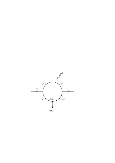
Figure 1: A contribution to the charged lepton dipole moments.

As it is shown in [13], inserting LFV radiative corrections to $A_{\ell}$ and $m_{\tilde{L}}^{2}$ in the diagram shown in Fig. (1), we obtain a contribution to the EDM of the corresponding charged lepton. By inserting one-loop lepton flavor violating corrections to $A_{\ell}$ and $m_{\tilde{L}}^{2}$, we obtain

$$\vec{d}_{i}^{\ (1)} = (-e)\eta_{d_{e}}m_{\ell i}{2\alpha\over(4\pi)^{5}}\sum_{a}\sum_{k,j,m}\left({V_{1a}\over c_{w}}\right)\left({V_{1a}\over c_{w}}+{V_{2a}\over s_{w}}\right){a_{0}m_{a}\over|m_{a}|^{6}}g({m^{2}_{\tilde{L}}\over m_{a}^{2}},{m^{2}_{\tilde{E}}\over m_{a}^{2}})$$ (6)

$$\cdot {\rm Im}[(Y_{\nu}^{ki})^{*}Y_{\nu}^{kj}(Y_{\nu}^{mj})^{*}Y_{\nu}^{mi}]\cdot(-2m_{0}^{2}{\rm Log}{M_{GUT}^{2}\over M_{k}^{2}})\vec{S},$$ (7)

where $\vec{S}$ is the spin of the lepton, $V$ is the mixing matrix of the neutralinos, $m_{a}$ are the masses of the neutralinos and

$$g(x_{L},x_{E}) = {1\over 2(x_{E}-x_{L})^{2}}\left({1-x_{L}^{2}+2x_{L}{\rm Log}x_{L}\over(1-x_{L})^{3}}-{1-x_{E}^{2}+2x_{E}{\rm Log}x_{E}\over(1-x_{E})^{3}}\right)$$ (8)

$$+ {1\over 2(x_{E}-x_{L})}\left({5-4x_{L}-x_{L}^{2}+2(1+2x_{L}){\rm Log}x_{L}\over(1-x_{L})^{4}}\right).$$ (9)

The main contribution to the diagram shown in Fig. (1) comes from the momenta around the supersymmetry breaking scale ($M_{susy}$); as a result we have to insert the values of $\Delta A_{\ell}$ and $\Delta m_{\tilde{L}}^{2}$ at $M_{susy}$ by taking into account the effects of running of the effective operators from the scale that the right-handed neutrinos decouple down to $M_{susy}$. It can be shown that the LFV corrections to the slepton masses remain unchanged between the two scales. However, lowering energy from the right-handed neutrino scale down to $M_{susy}$, $\Delta A_{\ell}$ changes significantly. Here, the main effect comes from the gauge interaction and we can practically neglect the effects of $Y_{\ell}$ on the running. The factor $\eta_{d_{e}}\simeq 1.5$ in Eq. (7) takes care of the running of $\Delta A_{\ell}$.

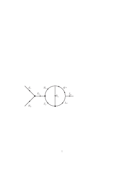
Figure 2: The two-loop correction to $A_{\ell}$ given by $m_{1/2}$. Vertices marked with circles are Yukawa vertices and the rest are gauge vertices. $F_{L_{i}}$ is the auxiliary field associated with $L_{i}$.

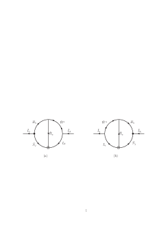
Figure 3: The two-loop corrections to $m_{\tilde{L}}$ given by $m_{1/2}$. Vertices marked with $\otimes$ and circles are Yukawa vertices and $A$-terms, respectively. The rest are gauge vertices.

Now, let us discuss the running of the relevant parameters from the GUT scale down to the right-handed neutrino scale. Let us take $M_{GUT}=2\times 10^{16}$ GeV and $M_{N}\sim Y_{\nu}^{2}\langle H_{u}\rangle^{2}/m_{\nu}$. For $Y_{\nu}\sim 1$ and $m_{\nu}\sim 0.1$ eV, we find $M_{N}\sim 10^{14}$ GeV so we expect that the running of parameters from the GUT scale down to the right-handed neutrino mass scale to be suppressed by ${\rm Log}(M_{N}^{2}/M_{GUT}^{2})/(16\pi^{2})\sim 0.1$. Thus, we can practically neglect the running of the gauge and Yukawa couplings as well as the gaugino and right-handed neutrino masses in this range. But there is a subtlety to be noted here. Although the dominant terms of both $\Delta A_{\ell}$ and $\Delta m_{\tilde{L}}^{2}$ are enhanced by a large log factor ${\rm Log}{M_{GUT}^{2}\over M_{k}^{2}}$, the effect in Eq. (7), which is given by ${\rm Im}(\Delta A_{\ell}\Delta m_{\tilde{L}}^{2})$, contains only one factor of ${\rm Log}{M_{GUT}^{2}\over M_{k}^{2}}$. This is because the leading-log parts of $\Delta A_{\ell}$ and $\Delta m_{\tilde{L}}^{2}$ have the same flavor structure $\sum_{k}(Y_{\nu}^{ki})^{*}{\rm Log}(M_{GUT}^{2}/M_{k}^{2})Y_{\nu}^{kj}$, and thus, ${\rm Im}\left[(\Delta A_{\ell})_{leading-log}(\Delta m_{\tilde{L}}^{2})_{leading-log}\right]=0$ and the dominant contribution to ${\rm Im}[\Delta A_{\ell}\Delta m_{\tilde{L}}^{2}]$ comes from ${\rm Im}\left[(\Delta A_{\ell})_{leading-log}(\Delta m_{\tilde{L}}^{2})_{finite}\right]$ and ${\rm Im}\left[(\Delta A_{\ell})_{finite}(\Delta m_{\tilde{L}}^{2})_{leading-log}\right]$ which contain only one large log factor. If there is a two-loop contribution to the $A_{\ell}$ term or mass matrix of the left-handed sleptons $\left[(\Delta A_{\ell})_{2-loop}\right.$ or $\left.(\Delta m_{\tilde{L}}^{2})_{2-loop}\right]$ with two large-log factors, ${\rm Im}[\Delta A_{\ell}^{2-loop}(\Delta m_{\tilde{L}}^{2})^{1-loop}_{L-L})]$ and ${\rm Im}[(\Delta A_{\ell})^{1{\rm-}loop}_{L-L}(\Delta m_{\tilde{L}}^{2})^{2-loop})]$ (here $L-L$ indices denote leading-log contributions) can be comparable to ${\rm Im}\left[(\Delta A_{\ell})_{L-L}^{1-loop}(\Delta m_{\tilde{L}}^{2})_{finite}^{1-loop}\right].$ Consequently, inserting the 2-loop correction to $A_{\ell}$ and 1-loop correction to $\Delta m_{\tilde{L}}^{2}$ (or vice-versa) in the diagram shown in Fig (1), we get an effect comparable to (or dominant over) Eq. (7). The diagrams shown in Figs. (2) and (3) give the dominant two-loop corrections to ($\Delta A_{\ell}$) and ($\Delta m_{\tilde{L}}^{2}$), respectively. The leading-log parts of the diagrams are

$$(\Delta A_{\ell})_{ik}=\frac{3}{2}m_{1/2}\frac{g^{2}}{(4\pi)^{4}}\sum_{j}Y_{\ell}^{i}(Y_{\nu}^{ji})^{*}Y_{\nu}^{jk}\left({\rm Log}\frac{M_{GUT}^{2}}{M_{j}^{2}}\right)^{2}$$ (10)

and

$$(\Delta m_{\tilde{L}}^{2})_{ik}=3m_{1/2}a_{0}\frac{g^{2}}{(4\pi)^{4}}\sum_{j}(Y_{\nu}^{ji})^{*}Y_{\nu}^{jk}\left({\rm Log}\frac{M_{GUT}^{2}}{M_{j}^{2}}\right)^{2}.$$ (11)

Inserting these diagrams in the diagram shown in Fig (1) we arrive at the following result

$$\vec{d}_{i}^{\ (2)} = (-e)\eta_{d_{e}}m_{\ell i}{-2\alpha\over(4\pi)^{7}}\frac{3g^{2}}{2}\sum_{a}\sum_{k,j,m}\left({V_{1a}\over c_{w}}\right)\left({V_{1a}\over c_{w}}+{V_{2a}\over s_{w}}\right){m_{1/2}m_{a}\over|m_{a}|^{6}}g({m^{2}_{\tilde{L}}\over m_{a}^{2}},{m^{2}_{\tilde{E}}\over m_{a}^{2}})$$ (12)

$$\cdot {\rm Im}[(Y_{\nu}^{ki})^{*}Y_{\nu}^{kj}(Y_{\nu}^{mj})^{*}Y_{\nu}^{mi}]\cdot(3m_{0}^{2}-a_{0}^{2})\left({\rm Log}{M_{GUT}^{2}\over M_{k}^{2}}\right)^{2}{\rm Log}{M_{GUT}^{2}\over M_{m}^{2}}\vec{S}.$$ (13)

This effect had been overlooked in the literature.

Finally, as discussed in [13], in large $\tan\beta$ domain the dominant contribution takes the following form:

$$\vec{d}_{i}^{\ (3)} = e{8\alpha\over(4\pi)^{7}}\sum_{a}\left({V_{1a}\over c_{w}}\right)\left({V_{1a}\over c_{w}}+{V_{2a}\over s_{w}}\right){\mu m_{\ell i}m_{a}\over|m_{a}|^{8}v^{2}}{\tan\beta\over\cos^{2}\beta}(9m_{0}^{4}+9a_{0}^{2}m_{0}^{2}+2a_{0}^{4})h(\frac{m_{\tilde{L}}^{2}}{m_{a}^{2}},\frac{m_{\tilde{E}}^{2}}{m_{a}^{2}})$$ (14)

$$\cdot \sum_{kjm}{\rm Im}[(Y_{\nu}^{ki})^{*}Y_{\nu}^{kj}m_{\ell j}^{2}(Y_{\nu}^{mj})^{*}Y_{\nu}^{mi}]\left({\rm Log}\frac{M_{GUT}^{2}}{M_{k}^{2}}\right)^{2}{\rm Log}{M_{GUT}^{2}\over M_{m}^{2}}\vec{S},$$ (15)

where

$$h(x_{L},x_{E}) = -{1\over(x_{E}-x_{L})^{3}}\left({1-x_{L}^{2}+2x_{L}{\rm Log}x_{L}\over(1-x_{L})^{3}}-{1-x_{E}^{2}+2x_{E}{\rm Log}x_{E}\over(1-x_{E})^{3}}\right)$$ (16)

$$- {1\over 2(x_{E}-x_{L})^{2}}\left({5-4x_{L}-x_{L}^{2}+2(1+2x_{L}){\rm Log}x_{L}\over(1-x_{L})^{4}}\right.$$ (18)

$$\left.+{5-4x_{E}-x_{E}^{2}+2(1+2x_{E}){\rm Log}x_{E}\over(1-x_{E})^{4}}\right).$$

Note that one should insert the value of $\mu$ at the supersymmetry breaking scale in Eq. (15).

To evaluate the order of magnitude of the EDMs, at first sight it seems that we can simply set all the supersymmetric parameters to some common scale $m_{susy}$ and take the values of the functions $f$ and $h$ in Eqs. (7,13,15) to be numbers of order 1. However, this is not a valid simplification because the functions $f$ and $h$ rapidly decrease when their arguments fall below unity. In the mSUGRA model we expect the mass of the lightest neutralino to be smaller than that of sfermions. As a result, we expect $h$ and $g$ to be smaller than one. In section 4, we will see that this effect gives rise to a suppression by two to three orders of magnitude.

3 Effects of the phases of $\mu$ and $a_{0}$ on EDMs

In this section, we first review the current bounds on $d_{e}$, $d_{\mu}$, $d_{D}$, $d_{Hg}$ and $d_{n}$ and the prospects of improving them. We then review how we can write them in terms of Im$(\mu)$ and Im$(a_{0})$.

• Electron EDM $d_{e}$: The present bound on the EDM of electron is

  $$d_{e}<1.7\times 10^{-27}\ \ e~{}{\rm cm}\,\ \ \mbox{at}\,\ \ 95~{}\%\ {\rm CL}\ \cite[cite]{[\@@bibref{}{pdg}{}{}]}$$ (19)

  DeMille and his Yale group are running an experiment that uses the PbO molecules to probe $d_{e}$. Within three years they can reach a sensitivity of $10^{-29}$ e cm [19] and hopefully down to a sensitivity of $10^{-31}$ e cm within five years. There are proposals [20] for probing $d_{e}$ down to $10^{-35}$ e cm level. In sum there is a very good prospect of measuring $d_{e}$ in future [21].

• Neutron EDM $d_{n}$: The present bound on $d_{n}$ [22] is

  $$d_{n}<6.3\times 10^{-26}e~{}cm\ \ {\rm at}\ \ 90\%\ \ {\rm C.L.}$$ (20)

  This bound will be improved considerably by LANSCE [23] which will be able to probe $d_{n}$ down to $4\times 10^{-28}$ e cm.

• Muon EDM, $d_{\mu}$: The present bound on $d_{\mu}$ [18] is

  $$d_{\mu}<7\times 10^{-19}~{}e~{}cm.$$ (21)

  There are proposals to measure $d_{\mu}$ down to $10^{-24}$ e cm [24]. Using the storage ring of a neutrino factory, measurement of $d_{\mu}$ down to $5\times 10^{-26}$ will become a possibility [25].

• Mercury EDM $d_{Hg}$: The present bound on $d_{Hg}$ is

  $$|d_{Hg}|<2.1\times 10^{-28}e~{}cm$$ (22)

  which can be improved by a factor of four [26].

• Deuteron EDM $d_{D}$: The present bound on $d_{D}$ is very weak; however, there are proposals [17] to probe $d_{D}$ down to

  $$|d_{D}|<(1-3)\times 10^{-27}~{}e~{}cm.$$ (23)

Different sources of CP-violation affect the EDMs listed above differently. As a result, in principle by combining the information on these observables, we can discriminate between different sources of CP-violation. However to perform such an analysis we must be able to express the EDMs in terms of Im$[a_{0}]$, Im$[\mu]$ and Im$[Y_{\nu}]$. In the previous section, we reviewed the effects of complex $Y_{\nu}$ on $d_{e}$. The effects of complex $a_{0}$ and $\mu$ on $d_{e}$ are also well understood. However, writing $d_{n}$, $d_{Hg}$ and $d_{D}$ in terms of the sources of CP-violation is more complicated. To do so, we first have to express $d_{n}$, $d_{Hg}$ and $d_{D}$ in terms of the EDMs and CEDMs of light quarks (namely, $d_{u}$, $d_{d}$, $d_{s}$, $\tilde{d}_{u}$, $\tilde{d}_{d}$ and $\tilde{d}_{s}$) and then calculate the quark EDMs and CEDMs in terms of Im$[a_{0}]$, Im$[\mu]$ and Im$[Y_{\nu}]$. The quark EDMs and CEDMs in terms of Im$[a_{0}]$ and Im$[\mu]$ have already been calculated in the literature. In this paper we have used the results of Ref. [27]. As we discussed in the appendix, the effects of Im$[Y_{\nu}]$ on the quark EDMs and CEDMs are negligible. Unfortunately, the first step (expressing $d_{n}$, $d_{Hg}$ and $d_{D}$ in terms of the quark EDMs and CEDMs) is quite challenging. Let us consider them one by one.

• $d_{n}(d_{q},\tilde{d}_{q})$:
  Despite of the rich literature on $d_{n}$ in terms of the quark EDMs and CEDMs, the results are quite model dependent. For example, the SU(3) chiral model [28] and QCD sum rules [29] predict different contributions from $\tilde{d}_{u}$ and $\tilde{d}_{d}$ to $d_{n}$. Considering these discrepancies in the literature, in this paper we do not use bounds on $d_{n}$ in our analysis. As it is shown in [30], information on $d_{n}$ can help to refute the “cancelation” scenario. We will come back to this point later.

• $d_{Hg}(d_{q},\tilde{d}_{q})$:
  There is an extensive literature on $d_{Hg}$ [31]. In this paper, following Ref. [32], we will interpret the bound on $d_{Hg}$ as

  $$|\tilde{d}_{d}-\tilde{d}_{u}|<2\times 10^{-26}~{}{\rm cm}.$$ (24)

  As shown in the recent paper [33], the EDM of electrons in the mercury atom can give a non-negligible contribution to $d_{Hg}$. As a result, improvements on the bound on $d_{Hg}$ will not be very helpful for us to discriminate between different sources of CP-violation; i. e., $d_{Hg}$ also obtains a correction from complex $Y_{\nu}$ through $d_{e}$.

• $d_{D}(d_{q},\tilde{d}_{q})$:
  Searches for $d_{D}$ can serve as an ideal probe for the existence of sources of CP-violation other than complex $Y_{\nu}$ because $i)$ there is a good prospect of improving the bound on $d_{D}$ [17]; $ii)$ an ionized deuteron does not contain any electrons and hence we expect only a negligible and undetectable contribution from $Y_{\nu}$ to $d_{D}$.

  To calculate $d_{D}$ in terms of quark EDMs and CEDMs, two techniques have been suggested in the literature: $i)$ QCD sum rules [34] and $ii)$ SU(3) chiral theory [28]. Within the error bars, the two models agree on the contribution from $\tilde{d}_{d}-\tilde{d}_{u}$ which is the dominant one. However, the results of the two models on the sub-dominant contributions are not compatible. Apart from this discrepancy, there is a large uncertainty in the contribution of the dominant term:

  $$d_{D}(d_{q},\tilde{d}_{q})\simeq-e(\tilde{d}_{u}-\tilde{d}_{d})\,5^{+11}_{-3}\ .$$ (25)

  In this paper we take “the best fit” for our analysis.

4 Numerical analysis

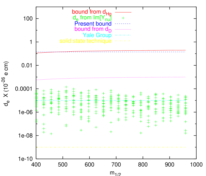
Figure 8: The same as fig. 7 for $a_{0}=1000$ GeV, $\tan\beta=20$ and sgn($\mu)=+$.

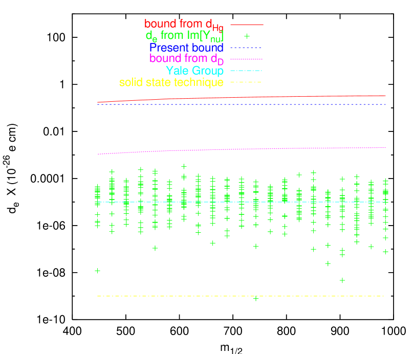
Figure 9: Electric dipole moment of the electron for $a_{0}=2000$ GeV, $\tan\beta=20$ and sgn($\mu)=+$. To draw the red solid and purple dotted lines, we have assumed that Im[$\mu$] is the only source of CP-violation and have taken $\tilde{d}_{d}-\tilde{d}_{u}$ equal to $2\times 10^{-26}$ cm and $2\times 10^{-28}$ cm, respectively to derive Im[$\mu$]. To produce the dots, we have assumed that complex $Y_{\nu}$ is the only source of CP-violation and have randomly produced $Y_{\nu}$ compatible with the data. The blue dashed line is the present bound on $d_{e}$ [18] and dot-dashed lines show the values of $d_{e}$ that can be probed in the future [19, 20]

In this section, we first describe how we produce the random seesaw parameters compatible with the data. We then describe the figs. (4-9) and, in the end, discuss what can be inferred from the future data considering different possible situations one by one.

In figures (4-9), the dots marked with ”+” represent $d_{e}$ resulting from complex $Y_{\nu}$. To extract random $Y_{\nu}$ and $M_{N}$ compatible with data, we have followed the recipe described in [35] and solved the following two equations

$$\eta_{m_{\nu}}Y_{\nu}^{T}{1\over M}Y_{\nu}(v^{2}\sin^{2}\beta)/2=U\cdot\Phi\cdot M_{\nu}^{Diag}\cdot\Phi\cdot U^{T}$$ (26)

and

$$h\equiv Y_{\nu}^{\dagger}{\rm Log}{M_{GUT}\over M}Y_{\nu}=\left[\matrix{a&0&d\cr 0&b&0\cr d^{*}&0&c}\right],$$ (27)

where $v=247$ GeV, $M$ is the mass matrix of the right-handed neutrinos, $U$ is the mixing matrix of neutrinos with $s_{13}=0$ and $\Phi$ is $diag[1,e^{i\phi_{1}},e^{i\phi_{2}}]$ with random values of $\phi_{1}$ and $\phi_{2}$ in the range $(0,2\pi)$. Finally, $M_{\nu}^{Diag}=diag[m_{1},\sqrt{m_{1}^{2}+\Delta m_{21}^{2}},\sqrt{m_{1}^{2}+\Delta m_{31}^{2}}]$ where $m_{1}$ picks up random values between 0 and 0.5 eV in a linear scale. The upper limit on $m_{1}$ is what has been found in [36] by taking the dark energy equation of state a free (but constant) parameter. In the above equation, $\eta_{m_{\nu}}$ takes care of the running of the neutrino mass matrix from $M$ to $M_{susy}$. Since the deviation of $\eta_{m_{\nu}}$ from unity is small [37], we have set $\eta_{m_{\nu}}=1$.

In order to satisfy the strong bounds on $\mbox{Br}(\mu\to e\gamma$) [18] and $\mbox{Br}(\tau\to\mu\gamma)$ [39], the matrix $h$, defined in Eq. (27), is taken to have this specific pattern with zero $e\mu$ and $\mu\tau$ elements. Actually these branching ratios put bounds on $(\Delta m_{\tilde{L}}^{2})_{e\mu}$ and $(\Delta m_{\tilde{L}}^{2})_{\mu\tau}$ rather than on $h_{e\mu}$ and $h_{\mu\tau}$. Notice that only the dominant term of $\Delta m_{\tilde{L}}^{2}$ is proportional to $h$. There is also a subdominant “finite” contribution to $\Delta m_{\tilde{L}}^{2}$ which is about 10% of the dominant effect and is not proportional to the matrix $h$ [13]. As we saw in section 2, this finite part plays a crucial role in giving rise to EDMs because the dominant leading-log part cancels out. Nonetheless, for extracting the seesaw parameters, 20% accuracy is enough and we can neglect the subdominant part and take $\Delta m_{\tilde{L}}^{2}$ proportional to the matrix $h$. In Eq. (27), $a$, $b$, $c$ are real numbers which take random values between 0 and 5. On the other hand, $|d|$ takes random values between 0 and the upper bound from $\mbox{Br}(\tau\to e\gamma)$ [40]. To calculate the upper bound on $|d|$, we have used the formulae derived in Ref. [41]. The phase of $d$ takes random values between 0 and 2$\pi$. With the above bounds on the random variables, the Yukawa couplings can be relatively large, giving rise to

$${\rm Im}\left[Y_{\nu}^{\dagger}{\rm Log}^{2}{M_{GUT}^{2}\over M_{N}^{2}}Y_{\nu}Y_{\nu}^{\dagger}{\rm Log}{M_{GUT}^{2}\over M_{N}^{2}}Y_{\nu}\right]_{ee}\sim{\rm few}\times 10$$ (28)

and

$${\rm Im}\left[Y_{\nu}^{\dagger}{\rm Log}{M_{GUT}^{2}\over M_{N}^{2}}Y_{\nu}Y_{\nu}^{\dagger}Y_{\nu}\right]_{ee}\sim{\rm few}\times 0.1.$$ (29)

As we discussed in the end of Sec. 2, because of the presence of the rapidly changing functions $g(x_{L},x_{R})$ and $h(x_{L},x_{R})$ in Eqs. (7, 13, 15), the value of $d_{e}$ strongly depends on the values of the supersymmetric parameters. To perform this analysis we have taken various values of $\tan\beta$ and $a_{0}$ and calculated the spectrum of the supersymmetric parameters along the $m_{1/2}-m_{0}$ strips parameterized in Ref. [42]. Notice that Ref. [42] has already removed the parameter range for which color or charge condensation takes place.

In the figures, we have also drawn the present bound on $d_{e}$ [18] as well as the limits which can be probed in the future. The present bound is shown by a dashed dark blue line and lies several orders of magnitude above the $d_{e}$ from phases of $Y_{\nu}$. After five years of data-taking, the Yale group can probe $d_{e}$ down to $10^{-31}$ e cm [19] which is shown with a dot-dashed cyan line in the figures. As it is demonstrated in the figures, only for large values of $a_{0}$ the effect of complex $Y_{\nu}$ on $d_{e}$ can be probed by the Yale group and for most of the parameter space the effect remains beyond the reach of this experiment.

There are proposals [20] to use solid state techniques to probe $d_{e}$ down to $10^{-35}$ e cm (shown with dot-dashed yellow line in the figure). In this case, as it can be deduced from the figure, we will have a great chance of being sensitive to the effects of the phases of $Y_{\nu}$ on $d_{e}$. However, unfortunately, the feasibility and time scale of the solid state technique is still uncertain.

Although for intermediate values of $\tan\beta$, the effect of the phases of $Y_{\nu}$ on $d_{e}$ is very low ($<10^{-30}$ e cm ), its effect can still be much higher than the four-loop effect on $d_{e}$ in the SM (the effect of the CP-violating phase of the CKM matrix) which is estimated to be $\sim 10^{-38}$ e cm [15].

In figs. (4-6) as well as in fig. 9, $d_{e}$ resulting from Im[$\mu$] is also depicted. The red solid lines in these figures show $d_{e}$ from Im[$\mu$] assuming that the corresponding $d_{Hg}$ saturates the present bound [26]. As it is well-known, there are uncertainties both in the value of $m_{d}$ [18] and in the interpretation of $d_{Hg}$ in terms of more fundamental parameters $\tilde{d}_{u}$, $\tilde{d}_{d}$ and $\tilde{d}_{s}$. To draw this curve we have assumed $m_{d}=5$ MeV and $\tilde{d}_{u}-\tilde{d}_{d}<2\times 10^{-26}$ e cm . As it is shown in the figure this bound is weaker than even the present direct bound on $d_{e}$. The purple dotted lines in figs. (4, 5, 6, 9), represent $d_{e}$ induced by values of Im$[\mu]$ that give rise to $\tilde{d}_{u}-\tilde{d}_{d}=2\times 10^{-28}$ cm (corresponding to $d_{D}=10^{-27}$ e cm and $d_{D}=5e(\tilde{d}_{d}-\tilde{d}_{u})$). Notice that these curves lie well below the direct bound on $d_{e}$ but the Yale group will be able to probe even smaller values of $d_{e}$. Similarly in figs. (7,8), $d_{e}$ resulting from Im[$a_{0}$] is depicted.

The following comments are in order:

1) The combination of the seesaw parameters that enter the formula for $d_{e}$ resulting from Im$[\Delta m_{\tilde{E}}^{2}m_{\ell}^{2}\Delta m_{\tilde{L}}^{2}]$ [see Eq. (15)] is

$${\rm Im}\left[Y_{\nu}^{\dagger}{\rm Ln}^{2}{M_{GUT}^{2}\over M^{2}}Y_{\nu}m_{\ell}^{2}Y_{\nu}^{\dagger}{\rm Ln}{M_{GUT}^{2}\over M^{2}}Y_{\nu}\right]_{ee}\simeq m_{\tau}^{2}{\rm Im}\left[\left(Y_{\nu}^{\dagger}{\rm Ln}^{2}{M_{GUT}^{2}\over M^{2}}Y_{\nu}\right)_{e\tau}\left(Y_{\nu}^{\dagger}{\rm Ln}{M_{GUT}^{2}\over M^{2}}Y_{\nu}\right)_{\tau e}\right]$$ (30)

where $M$ is the mass matrix of the right-handed neutrinos. In contrast to this, the “new” effect given in Eq. (13) is proportional to

$${\rm Im}\left[Y_{\nu}^{\dagger}{\rm Ln}^{2}{M_{GUT}^{2}\over M_{N}^{2}}Y_{\nu}Y_{\nu}^{\dagger}{\rm Ln}{M_{GUT}^{2}\over M_{N}^{2}}Y_{\nu}\right]_{ee}.$$

For the specific pattern of the $h$ matrix shown in Eq. (27) (with zero $e\mu$ element) this effect is also given by

$${\rm Im}\left[\left(Y_{\nu}^{\dagger}{\rm Ln}^{2}{M_{GUT}^{2}\over M_{N}^{2}}Y_{\nu}\right)_{e\tau}\left(Y_{\nu}^{\dagger}{\rm Ln}{M_{GUT}^{2}\over M_{N}^{2}}Y_{\nu}\right)_{\tau e}\right].$$ (31)

In other words, the two effects are proportional to each other.

For the values of supersymmetric parameters chosen in Fig. (4) (that is, sgn($\mu$)=+, $\tan\beta=10$, $a_{0}=0$), the ”new” effect is dominant and is $-5$ times the effect previously discussed in the literature. However, for $a_{0}=1000$ GeV and 2000 GeV (Figs. 7,8 and 9) the dominant contribution is the one given by Eq. (15).

2) In the figures, the bounds from $d_{Hg}$ and $d_{D}$ appear almost as horizontal lines. This results from the fact that for the $m_{0}-m_{1/2}$ strips that we analyze, $m_{0}$ is almost proportional to $m_{1/2}$. Using dimensional analysis we can write

$$\tilde{d}_{u}-\tilde{d}_{d}\simeq k_{1}{{\rm Im}[\mu]\ \ {\rm or\ \ Im}[a_{0}]\over m_{1/2}^{3}}\ \ \ \ \ \ d_{e}\simeq k_{2}{{\rm Im}[\mu]\ \ {\rm or\ \ Im}[a_{0}]\over m_{1/2}^{3}}$$

where $k_{1}$ and $k_{2}$ are given by the relevant fermion masses and are independent of $m_{1/2}$. As a result, for a given value of $\tilde{d}_{u}-\tilde{d}_{d}$, Im[$\mu$] (or Im[$a_{0}$]) itself is proportional to $m_{1/2}^{3}$ so $d_{e}$ will not vary with $m_{1/2}$.

3) As discussed in Ref. [43], at two-loop level, the imaginary $a_{0}$ can induce an imaginary correction to the Wino mass, giving rise to another contribution to the EDMs. In our analysis, we have taken this effect into account but it seems to be subdominant.

In the following, we will discuss what can be inferred about the sources of CP-violation from $d_{e}$ and $d_{D}$ if their values (or the bounds on them) turn out to be in certain ranges.

According to the Figs. (4-6), for $a_{0}=0$, any signal found by the Yale group implies that there are sources of CP-violation other than the phases of the Yukawa couplings. However, for larger values of $a_{0}$, the effect of $Y_{\nu}$ on the EDMs can be observed by the Yale group within five years. According to Figs. (7-9), for $a_{0}\mathop{}_{\textstyle\sim}^{\textstyle>}1000$ GeV EDMs originating from complex $Y_{\nu}$ can be large enough to be observed by the Yale group. Therefore, if after five years the Yale group reports a null result, we can derive bounds on certain combinations of seesaw parameters and $a_{0}$. At least it will be possible to discriminate between low and high $a_{0}$ values. If after five years the Yale group reports a null result, we can derive bounds on the seesaw parameters. However, if the Yale group finds that $10^{-31}~{}e~{}{\rm cm}<d_{e}<10^{-29}$ e cm we will not be able to determine whether $d_{e}$ originates from complex $Y_{\nu}$ or from more familiar sources such as complex $a_{0}$ or $\mu$. To be able to make such a distinction, values of $d_{D}$ down to $10^{-28}-10^{-29}$ e cm have to be probed which, at the moment, does not seem to be achievable.

If future searches for $d_{D}$ find $d_{D}>10^{-27}$ e cm but the Yale group finds $d_{e}<2\times 10^{-29}$ e cm (this can be tested within only 3 years of data taking by the Yale group [19]), we might conclude that the source of CP-violation is something other than pure Im$[\mu]$ or Im$[a_{0}]$; e.g., QCD $\theta$-term which can give a significant contribution to $d_{D}$ but only a negligible contribution to $d_{e}$. Another possibility is that there is a cancelation between the contributions of Im$[\mu]$ and Im$[a_{0}]$ to $d_{e}$. The information on $d_{n}$ would then help us to resolve this ambiguity provided that the theoretical uncertainties in calculation of $d_{n}$ as well as $d_{D}$ are sufficiently reduced.

On the other hand, if the Yale group detects $d_{e}>2\times 10^{-29}$ e cm, we will expect that $d_{D}>10^{-27}$ e cm which will be a strong motivation for building a deuteron storage ring and searching for $d_{D}$. If such a detector finds a null result, within this framework the explanation will be quite non-trivial requiring some fine-tuned cancelation between different contributions.

According to these figures, in the foreseeable future, we will not be able to extract any information on the seesaw parameters from EDMs, because even if we develop techniques to probe $d_{e}$ as small as $10^{-35}\,{\rm e-cm}$, we will not be able to subtract (or dismiss) the effect coming from Im$[\mu]$ and Im$[a_{0}]$ unless we are able to probe $\tilde{d}_{u}-\tilde{d}_{d}$ at least 5 orders of magnitude below its present bound which seems impractical. Remember that this is under the optimistic assumptions that the mass of the lightest neutrino, $m_{1}$, and $\mbox{Br}(\tau\to e\gamma)$ are close to their upper bounds and there is no cancelation between different contributions to the EDMs.

If, in the future, we realize that $m_{1}$ and $\mbox{Br}(\tau\to e\gamma)$ are indeed close to the present upper bounds on them and $a_{0}=0$ ($a_{0}=1000\ {\rm GeV}$) but find $d_{e}<10^{-35}$e cm ($d_{e}<10^{-34}$ e cm ), we will be able to draw bounds on the phases of $Y_{\nu}$ which along with the information on the phases of the Dirac and Majorana phases of the neutrino mass matrix and the CP-violating phase of the left-handed slepton mass matrix may have some implication for leptogenesis. This is however quite an unlikely situation.

Let us now discuss the $d_{\mu}$. As we saw in Sec. 2, the phases of $Y_{\nu}$ manifest themselves in the $d_{\mu}$ through Im$[\Delta A_{\ell}\Delta m_{\tilde{L}}^{2}]_{\mu\mu}$ and Im$[\Delta m_{\tilde{E}}^{2}m_{\ell}^{2}\Delta m_{\tilde{L}}^{2}]_{\mu\mu}$. If $a_{0}$ is a real number, the matrix $A_{\ell}$ remains Hermitian [13]. That is the radiative corrections due to $Y_{\nu}$ cannot induce nonzero Im$[\Delta A_{\ell}]_{ii}$. So, we can write

$${\rm Im}[\Delta A_{\ell}\Delta m_{\tilde{L}}^{2}]_{\mu\mu}={\rm Im}[(\Delta A_{\ell})_{\mu e}(\Delta m_{\tilde{L}}^{2})_{e\mu}]+{\rm Im}[(\Delta A_{\ell})_{\mu\tau}(\Delta m_{\tilde{L}}^{2})_{\tau\mu}]$$

and

$${\rm Im}[\Delta m_{\tilde{E}}^{2}m_{\ell}^{2}\Delta m_{\tilde{L}}^{2}]_{\mu\mu}={\rm Im}[(\Delta m_{\tilde{E}}^{2})_{\mu e}m_{e}^{2}(\Delta m_{\tilde{L}}^{2})_{e\mu}]+{\rm Im}[(\Delta m_{\tilde{E}}^{2})_{\mu\tau}m_{\tau}^{2}(\Delta m_{\tilde{L}}^{2})_{\tau\mu}].$$

The strong bounds on $\mbox{Br}(\mu\to e\gamma$) [18] and $\mbox{Br}(\tau\to\mu\gamma$) [39] can be translated into bounds on $(\Delta m_{\tilde{L}}^{2})_{e\mu}$ and $(\Delta m_{\tilde{L}}^{2})_{\tau\mu}$ as well as the corresponding elements of $\Delta A_{\ell}$. As a result, in the framework that imaginary $Y_{\nu}$ is the only source of CP-violation, we expect

$$d_{\mu}\sim d_{e}\frac{m_{\mu}}{m_{e}}{(\Delta m_{\tilde{L}}^{2})_{\tau\mu}\over(\Delta m_{\tilde{L}}^{2})_{\tau e}}<10^{-31}~{}e~{}{\rm cm},$$

which will not be observable even if the muon storage ring of a nu-factory is built [25]. On the other hand, imaginary $a_{0}$ and $\mu$ induce $d_{\mu}\sim d_{e}m_{\mu}/m_{e}$ and allow $d_{e}$ to be as large as the experimental upper bound on it. In this case, we may have a chance of observing $d_{\mu}$. Observing $d_{\mu}\gg m_{\mu}d_{e}/m_{e}$ will indicate that this simplified version of the MSSM is not valid.

5 Summary and conclusions

In this work we have studied EDMs of particles in the context of supersymmetric seesaw mechanism. We have examined various contributions to electron EDM induced by the CP–odd phases in the neutrino Yukawa matrix. Our analysis takes into account various contributions available in the literature as well as a new one, proportional to the gaugino masses, which is presented in Eq. (13).

In our discussions we have first produced random complex neutrino Yukawa couplings consistent with the bounds from LFV rare decays and then calculated the electron EDM they induce along post-WMAP $m_{0}-m_{1/2}$ strips for given values of $\tan\beta$ and $a_{0}$ [42]. We have found that, for small values of $a_{0}$, the new contribution (13) can be dominant over the other contributions from $Y_{\nu}$ that had already been studied in the literature.

It turns out that for a realistic mass spectrum of supersymmetric particles, there is an extra suppression factor of $10^{-2}-10^{-3}$ with which we would not encounter if all the supersymmetric masses were taken to be equal to each other. In figs. 4-9, the values of $d_{e}$ corresponding to different random complex $Y_{\nu}$ textures are represented by dots. For small values of $\tan\beta$ ($\tan\beta<10$) and $a_{0}$ ($a_{0}<1000$ GeV), $d_{e}$ induced by $Y_{\nu}$ is beyond the reach of the ongoing experiments [19]. Such values of $d_{e}$ can however be probed by the proposed solid state based experiments [20]. For larger values of $\tan\beta$ and/or $a_{0}$, the Yale group may be able to detect the effects of complex $Y_{\nu}$ on $d_{e}$. As it is demonstrated in Figs. 8 and 9, for $\tan\beta=20$ and $a_{0}=1000-2000$ GeV, a large fraction of parameter space yields $d_{e}$ detectable by the Yale group. However, even in this case we will not be able to extract information on the seesaw parameters from $d_{e}$ because the source of CP-violation might be $a_{0}$ and/or $\mu$ rather than $Y_{\nu}$. If the future searches for $d_{D}$ [34] find out that $d_{D}>10^{-27}$ e cm then we will conclude that there is a source of CP-violation other than complex $Y_{\nu}$. However, to prove that the dominant contribution to $d_{e}$ detected by the Yale group comes from complex $Y_{\nu}$– hence to be able to extract information on the seesaw parameters from it– we should show that $d_{D}<10^{-28}-10^{-29}$ e cm which is beyond the reach of even the current proposals. Notice that for the purpose of discriminating between complex $Y_{\nu}$ and $a_{0}/\mu$ as sources of CP-violation, searching for $d_{Hg}$ is not very helpful because mercury atom contains electron and hence $d_{Hg}$ obtains a contribution from complex $Y_{\nu}$. That is while ionized deuteron used for measuring $d_{D}$ does not contain any electron and the contribution of complex $Y_{\nu}$ to it is negligible. To obtain information from $d_{n}$, the theoretical uncertainties first have to be resolved.

In this paper, we have also shown that for the neutrino Yukawa couplings satisfying the current bounds from the LFV rare decays, the electric dipole moment of muon induced by $Y_{\nu}$ is negligible and cannot be detected in the foreseeable future. Detecting a sizeable $d_{\mu}$ will indicate that there are sources of CP-violation beyond the complex $Y_{\nu}$.

6 Appendix

Since $d_{D}$ is dominantly given by $\tilde{d}_{d}-\tilde{d}_{u}$, in this section, we concentrate on evaluating $\tilde{d}_{q}$. One can repeat a similar discussion for $d_{q}$.

In Sec. 2, we saw that integrating out $N_{i}$, the effects of CP-violating phases appear in the left-right mixing of sleptons which can be evaluated to $m_{\ell}m_{susy}F(Y_{\nu},{\rm Log}[M_{GUT}^{2}/M^{2}])/(16\pi^{2})^{2}$ or for large $\tan\beta$, to $m_{\ell}m_{susy}\tan\beta(m_{\tau}^{2}\tan^{2}\beta/v^{2})F^{\prime}(Y_{\nu},{\rm Log}[M_{GUT}^{2}/M^{2}])/(16\pi^{2})^{2}$. For random $Y_{\nu}$ consistent with observed $m_{\nu}$ and bounds on the branching ratios of LFV rare decay, the functions $F$ and $F^{\prime}$ take values smaller than 0.1. Since quarks do not directly couple to the leptonic sector, the CP-violation in the leptonic sector should be transferred to the quark sector through one-loop (or higher loop) effective operators made of Higgs and gauge bosons or their superpartners. To construct such an effective operator one more factor of $Y_{\ell}$ is needed to compensate for the left-right mixing mentioned above. Considering the fact that $Y_{\tau}\gg Y_{\mu},Y_{e}$, the main contribution to the effective operator comes from the diagrams with $\tau$ and $\tilde{\tau}$ propagating in them. So the CP-odd effective potential will be given by

$$m_{susy}^{n}m_{\tau}^{2}\tan\beta F(Y_{\nu},{\rm Log}[M_{GUT}^{2}/M^{2}])/(16\pi^{2})^{3}$$

or for large $\tan\beta$,

$$m_{susy}^{n}m_{\tau}^{2}\tan^{2}\beta(m_{\tau}^{2}\tan^{2}\beta/v^{2})F^{\prime}(Y_{\nu},{\rm Log}[M_{GUT}^{2}/M^{2}])/(16\pi^{2})^{3}.$$

In these formula, the power of $m_{susy}$, $n$, is determined by the dimension of the specific operator under consideration.

To evaluate $\tilde{d}_{q}$, we have to insert the CP-odd effective operator in another one-loop diagram. Since CEDMs mix left- and right-handed, the latter diagram should involve a factor of $Y_{q}$. So, we can write

$$\tilde{d}_{q}\sim{Y_{q}g^{2}g_{s}\over 16\pi^{2}}{m_{\tau}^{2}\tan\beta F(Y_{\nu},{\rm Log}[M_{GUT}^{2}/M^{2}])\over(16\pi^{2})^{3}m_{susy}^{3}}$$

and for large $\tan\beta$,

$$\tilde{d}_{q}\sim{Y_{q}g^{2}g_{s}\over 16\pi^{2}}{m_{\tau}^{2}\tan^{2}\beta(m_{\tau}^{2}\tan^{2}\beta/v^{2})F^{\prime}(Y_{\nu},{\rm Log}[M_{GUT}^{2}/M^{2}])\over(16\pi^{2})^{3}m_{susy}^{3}}.$$

As a result, we expect $\tilde{d}_{d}<10^{-30}$ cm which cannot be observed even if the recent proposal [17] is implemented. We expect $\tilde{d}_{u}$ to be even smaller because $Y_{u}/Y_{d}=m_{u}/m_{d}\cot\beta\ll 1$. Notice that although $\tilde{d}_{q}$ is suppressed by a factor of $m_{\tau}^{2}\tan^{2}\beta/(16\pi^{2}m_{susy}^{2})$, $e\tilde{d}_{d}$ can be comparable to $d_{e}$. This originates from two facts: $Y_{d}/Y_{e}\sim 10$ and in the case of $d_{e}$, as we discussed in Sec. 2, there is an extra suppression given by the functions $g(x_{L},x_{E})$ and $h(x_{L},x_{E})$. If we do precise two-loop calculation of $\tilde{d}_{d}$ for a realistic SUSY spectrum, we may encounter similar suppression. As the above analysis show we do not expect an observable effect due to $Y_{\nu}$ in future searches for $d_{D}$ and $d_{Hg}$ so it seems there is not a strong motivation for performing such a complicated two-loop calculation.

7 Acknowledgements

The research of D.D. was partially supported by GEBIP grant of the Turkish Academy of Sciences and by project 104T503 of Scientific and Technical Research Council of Turkey. The authors are grateful to J. Ellis and M. Peskin for the encouragement and useful discussions. Y. F. would like to thank A. Ritz for fruitful discussions. The authors also appreciate M. M. Sheikh-Jabbari for careful reading of the manuscript, and for useful comments.

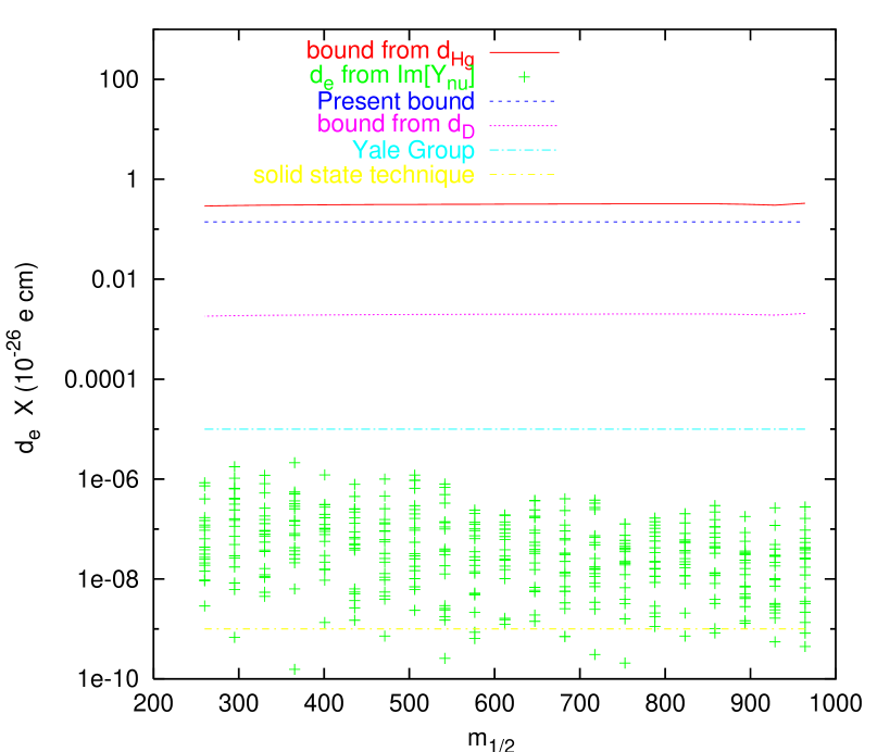
Figure 4: Electric dipole moment of the electron for $a_{0}=0$, $\tan\beta=10$ and sgn($\mu)=+$. To draw the red solid and purple dotted lines, we have assumed that Im[$\mu$] is the only source of CP-violation and have taken $\tilde{d}_{d}-\tilde{d}_{u}$ equal to $2\times 10^{-26}$ cm and $2\times 10^{-28}$ cm, respectively to derive Im[$\mu$]. To produce the dots, we have assumed that complex $Y_{\nu}$ is the only source of CP-violation and have randomly produced $Y_{\nu}$ compatible with the data. The blue dashed line is the present bound on $d_{e}$ [18] and dot-dashed lines show the values of $d_{e}$ that can be probed in the future [19, 20]

Figure 5: The same as fig. 4 for $a_{0}=0$, $\tan\beta=20$ and sgn($\mu)=+$.

Figure 6: The same as fig. 4 for $a_{0}=0$, $\tan\beta=20$ and sgn($\mu)=-$.

Figure 7: Electric dipole moment of the electron for $a_{0}=1000$ GeV, $\tan\beta=10$ and sgn($\mu)=+$. To draw the red solid and purple dotted lines, we have assumed that Im[$a_{0}$] is the only source of CP-violation and have taken $\tilde{d}_{d}-\tilde{d}_{u}$ equal to $2\times 10^{-26}$ cm and $2\times 10^{-28}$ cm, respectively to derive Im[$a_{0}$]. To produce the dots, we have assumed that complex $Y_{\nu}$ is the only source of CP-violation and have randomly produced $Y_{\nu}$ compatible with the data. The blue dashed line is the present bound on $d_{e}$ [18] and dot-dashed lines show the values of $d_{e}$ that can be probed in the future [19, 20]

References

- [1] see e.g., M. B. Smy et al. [Super-Kamiokande Collaboration], Phys. Rev. D 69 (2004) 011104 [arXiv:hep-ex/0309011]; S. N. Ahmed et al. [SNO Collaboration], Phys. Rev. Lett. 92 (2004) 181301 [arXiv:nucl-ex/0309004]; S. Moriyama [Super-Kamiokande Collaboration], Nucl. Phys. Proc. Suppl. 145 (2005) 112.
- [2] T. Araki et al. [KamLAND Collaboration], Phys. Rev. Lett. 94 (2005) 081801 [arXiv:hep-ex/0406035]; http://www.awa.tohoku.ac.jp/KamLAND.
- [3] http://superk.physics.sunysb.edu/k2k/
- [4] J. Bonn et al., Nucl. Phys. Proc. Suppl. 91 (2001) 273.
- [5] U. Seljak et al., arXiv:astro-ph/0407372; M. Tegmark et al. [SDSS Collaboration], Astrophys. J. 606 (2004) 702 [arXiv:astro-ph/0310725]; U. Seljak et al., Phys. Rev. D 71 (2005) 043511 [arXiv:astro-ph/0406594]; V. Barger, D. Marfatia and A. Tregre, Phys. Lett. B 595 (2004) 55 [arXiv:hep-ph/0312065].
- [6] A. Y. Smirnov, arXiv:hep-ph/0411194.
- [7] M. Gell-Mann, P. Ramond and R. Slansky, Print-80-0576 (CERN) (See also P. Ramond, arXiv:hep-ph/9809459); T. Yanagida, In Proceedings of the Workshop on the Baryon Number of the Universe and Unified Theories, Tsukuba, Japan, 13-14 Feb 1979; S. L. Glashow, HUTP-79-A059 Based on lectures given at Cargese Summer Inst., Cargese, France, Jul 9-29, 1979; R. N. Mohapatra and G. Senjanovic, Phys. Rev. Lett. 44 (1980) 912.
- [8] M. Fukugita and T. Yanagida, Phys. Lett. B 174 (1986) 45.
- [9] P. Nath, R. Arnowitt and A. H. Chamseddine, NUB-2613 Lectures given at Summer Workshop on Particle Physics, Trieste, Italy, Jun 20 - Jul 29, 1983.
- [10] F. Borzumati and A. Masiero, Phys. Rev. Lett. 57 (1986) 961.
- [11] S. Davidson and A. Ibarra, JHEP 0109 (2001) 013 [arXiv:hep-ph/0104076].
- [12] J. Hisano, D. Nomura and T. Yanagida, Phys. Lett. B 437 (1998) 351 [arXiv:hep-ph/9711348]; A. Romanino and A. Strumia, Nucl. Phys. B 622 (2002) 73 [arXiv:hep-ph/0108275]; J. R. Ellis, J. Hisano, M. Raidal and Y. Shimizu, Phys. Lett. B 528 (2002) 86 [arXiv:hep-ph/0111324]; I. Masina, Nucl. Phys. B 671 (2003) 432 [arXiv:hep-ph/0304299].
- [13] Y. Farzan and M. E. Peskin, Phys. Rev. D 70 (2004) 095001 [arXiv:hep-ph/0405214].
- [14] B. Dutta and R. N. Mohapatra, Phys. Rev. D 68 (2003) 113008 [arXiv:hep-ph/0307163]; I. Masina and C. A. Savoy, Phys. Rev. D 71 (2005) 093003 [arXiv:hep-ph/0501166].
- [15] M. E. Pospelov and I. B. Khriplovich, Sov. J. Nucl. Phys. 53 (1991) 638 [Yad. Fiz. 53 (1991) 1030].
- [16] Y. Farzan, Phys. Rev. D 69 (2004) 073009 [arXiv:hep-ph/0310055].
- [17] Y. K. Semertzidis et al. [EDM Collaboration], AIP Conf. Proc. 698 (2004) 200 [arXiv:hep-ex/0308063].
- [18] S. Eidelman et al., Phys. Lett B592 (2004) 1.
- [19] D. Kawall et al., electron in AIP Conf. Proc. 698 (2004) 192.
- [20] S. K. Lamoreaux, arXiv:nucl-ex/0109014.
- [21] J. J. Hudson et al., Phys. Rev. Lett. 89 (2002) 023003; Y. K. Semertzidis, hep-ex/0401016.
- [22] P. G. Harris et al., Phys. Rev. Lett. 82 (1999) 904.
- [23] http://p25ext.lanl.gov/edm/edm.html
- [24] Y. K. Semertzidis et al., arXiv:hep-ph/0012087.
- [25] J. Aysto et al., arXiv:hep-ph/0109217.
- [26] M. V. Romalis, W. C. Griffith and E. N. Fortson, Phys. Rev. Lett. 86 (2001) 2505 [arXiv:hep-ex/0012001].
- [27] T. Ibrahim and P. Nath, Phys. Rev. D 57 (1998) 478 [Erratum-ibid. D 58 (1998 ERRAT,D60,079903.1999 ERRAT,D60,119901.1999) 019901] [arXiv:hep-ph/9708456].
- [28] J. Hisano and Y. Shimizu, Phys. Rev. D 70 (2004) 093001 [arXiv:hep-ph/0406091].
- [29] M. Pospelov and A. Ritz, Phys. Rev. D 63 (2001) 073015 [arXiv:hep-ph/0010037].
- [30] T. Falk, K. A. Olive, M. Pospelov and R. Roiban, Nucl. Phys. B 560 (1999) 3 [arXiv:hep-ph/9904393].
- [31] J. Hisano, M. Kakizaki, M. Nagai and Y. Shimizu, Phys. Lett. B 604 (2004) 216 [arXiv:hep-ph/0407169]; T. Falk, K. A. Olive, M. Pospelov and R. Roiban, Nucl. Phys. B 560 (1999) 3 [arXiv:hep-ph/9904393].
- [32] M. Pospelov, Phys. Lett. B 530 (2002) 123 [arXiv:hep-ph/0109044].
- [33] M. Pospelov and A. Ritz, arXiv:hep-ph/0504231.
- [34] O. Lebedev, K. A. Olive, M. Pospelov and A. Ritz, Phys. Rev. D 70 (2004) 016003 [arXiv:hep-ph/0402023].
- [35] J. R. Ellis, J. Hisano, M. Raidal and Y. Shimizu, Phys. Rev. D 66 (2002) 115013 [arXiv:hep-ph/0206110].
- [36] S. Hannestad, arXiv:astro-ph/0505551.
- [37] S. Antusch, J. Kersten, M. Lindner and M. Ratz, Nucl. Phys. B 674 (2003) 401 [arXiv:hep-ph/0305273].
- [38] O. Lebedev, K. A. Olive, M. Pospelov and A. Ritz, Phys. Rev. D 70 (2004) 016003 [arXiv:hep-ph/0402023].
- [39] B. Aubert et al. [BABAR Collaboration], arXiv:hep-ex/0502032.
- [40] K. Hayasaka et al., Phys. Lett. B 613 (2005) 20 [arXiv:hep-ex/0501068].
- [41] T. Fukuyama, T. Kikuchi and N. Okada, Phys. Rev. D 68, 033012 (2003) [arXiv:hep-ph/0304190]; S. T. Petcov, S. Profumo, Y. Takanishi and C. E. Yaguna, Nucl. Phys. B 676 (2004) 453 [arXiv:hep-ph/0306195];
- [42] L. S. Stark, P. Hafliger, A. Biland and F. Pauss, arXiv:hep-ph/0502197.
- [43] K. A. Olive, M. Pospelov, A. Ritz and Y. Santoso, arXiv:hep-ph/0506106.