Loop corrections to the form factors in $B\to\pi l\nu$ decay

G.G. Kirilin

Budker Institute of Nuclear Physics SB RAS

630090 Novosibirsk, Russia

In this paper we study the semileptonic decay $B\to\pi l\nu$ and in particular the factorizable contribution to symmetry breaking corrections to the form factors at large recoil. This contribution is a convolution of the coefficient function, which can be calculated in perturbation theory, and of the nonperturbative light-cone distribution amplitudes of the mesons. The coefficient function, in turn, can also be represented as convolution of the hard Wilson coefficient and of the jet function. Loop corrections to the hard Wilson coefficient and jet function are calculated. We use the method of expanding by regions to calculate these corrections. The results obtained coincide with the ones calculated in the framework of the soft-collinear effective theory (SCET). Factorization of soft and collinear singularities into the light-cone distribution amplitudes is demonstrated at one-loop level explicitly. It is also demonstrated that the contribution of the so-called soft-messenger modes vanishes; this fact is of critical importance to the factorization approach to this decay.

PACS: 12.39.St, 14.65.Fy

1 Introduction

Recent advances in experimental investigation of heavy meson decays demand detailed theoretical analysis of these decays. Of prime importance are $B$-meson decays into light particles: pseudoscalar or vector mesons, photons and light lepton pairs, because the amplitudes of these decays are proportional to the non-diagonal elements of the CKM matrix.

Recently, consistent factorization approach has been developed for heavy-to-light transitions; it includes so-called soft-collinear effective theory (SCET) [1], [2]. This theory describes form factors of heavy-to-light transitions in the kinematical region with the energy of one or several light final state particles comparable with the $B$-meson mass. A typical example is the semileptonic decay $B\to\pi l\nu$. In first order in $G_{F}$ the amplitude of the decay is proportional to the matrix element of the vector current between $B$ and $\pi$ mesons. The matrix element can be written in terms of two form factors:

$$A^{\mu}=\left\langle\pi(q)\right|\bar{q}\gamma^{\mu}Q\left|B(p)\right\rangle\\ =f_{+}(t)\,\left(p^{\mu}+q^{\mu}-\frac{M_{B}^{2}-m_{\pi}^{2}}{t}\,(p-q)^{\mu}\right)+f_{0}(t)\,\frac{M_{B}^{2}-m_{\pi}^{2}}{t}(p-q)^{\mu}\,,$$ (1)

where $t=(p-q)^{2}$. Since $m_{\pi}\ll M_{b}$, we neglect the pion mass below.

Let us consider a frame where the momenta of the initial and final mesons take the form:

$$p=M_{B}\leavevmode\nobreak\ v=M_{B}\leavevmode\nobreak\ (1,0,0,0),\quad q=E\leavevmode\nobreak\ n=E(1,0,0,-1),$$ (2)

where $E$ is the energy of the pion. It is convenient to introduce one more light-cone vector:

$$n_{+}=(1,0,0,1),\quad v=\frac{n}{2}+\frac{n_{+}}{2}.$$ (3)

In this frame the amplitude (1) can be represented as follows:

$$A^{\mu}=\frac{M_{B}}{2}\left(f_{0}+f_{+}\leavevmode\nobreak\ z\right)\leavevmode\nobreak\ n^{\mu}+\frac{M_{B}}{2\leavevmode\nobreak\ \bar{z}}\left(f_{0}-f_{+}\leavevmode\nobreak\ z\right)\,n_{+}^{\mu}\,,$$ (4)

where $z=2E/M_{B},\bar{z}=1-z$. On the other hand, the matrix element can be written as

$$\left\langle\pi(q)\right|\bar{q}\gamma^{\mu}Q\left|B(p)\right\rangle=\frac{n^{\mu}}{2}\leavevmode\nobreak\ \left\langle\pi(q)\right|\bar{q}\,\not\!n_{+}\,Q\left|B(p)\right\rangle+\frac{n_{+}^{\mu}}{2}\,\left\langle\pi(q)\right|\bar{q}\,\not\!n\,Q\left|B(p)\right\rangle\,.$$ (5)

The kinematical region we are interested in is $z\sim 1$, i.e., the energy of the pion is of the order of the mass of the heavy meson $M_{B}\gg\Lambda_{\mathrm{QCD}}$. If hadronization occurs in such a way that the light quark produced in the decay of the heavy quark inside the $B$-meson has a virtuality of order $\Lambda_{\mathrm{QCD}}^{2}$ but this quark carries sufficiently large part of the pion energy, then this quark may be thought to be asymptotically free so that $\bar{q}\!\not\!\!n\approx 0$. In this case the last term in (5) vanishes. Comparing with (4) yields

$$zf_{+}(t)=f_{0}(t).$$ (6)

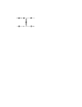
Expression (6) is known as the symmetry of the form factors at large recoil [3]. Apparently, a hard radiative correction, that affects the light quark, breaks this symmetry. In [4] possible ways of violating the symmetry were considered, namely, the radiative corrections to the ”non-factorizable” Feynman mechanism (Fig. 1a) and the hard spectator-scattering mechanism (Fig. 1b). The contribution of the latter factorizes into the product of the light-cone distribution amplitudes (LCDAs) of the mesons and the coefficient function. The difference of the form factors can be written [5], [6]

$$f_{0}-zf_{+}\,=\frac{\bar{z}}{M_{B}}\,\left\langle\pi\right|\bar{q}\not\!\!n\,Q\left|B\right\rangle=\mathcal{C}(E)\,\xi_{\pi}(E)+\int_{0}^{\infty}d\omega\,\Phi_{+}(\omega)\int_{0}^{1}du\,\phi_{\pi}(u)\,T(E,\omega,u),$$ (7)

where $\xi_{\pi}(E)$ is the universal nonperturbative form factor that corresponds to the Feynman mechanism, $\Phi^{+}(\omega),\,\phi_{\pi}(u)$ are the light-cone distribution amplitudes of the initial and final mesons. The form factors can be also represented in the form of Eq.7 [7], [6] but in this case the Wilson coefficient $\mathcal{C}(E)$ begins with $1$ instead of $\alpha_{s}$ as it does with the difference of the form factors (Fig. 1a).

(a)

(b)

Figure 1: Symmetry breaking radiative corrections

The coefficient function $T(E,\omega,u)$ is universal in the sense that it depends on initial and final states through the quantum numbers only. Consequently, this function can be calculated by considering the scattering amplitude of the partons that constitute the final and initial mesons:

$$A(E,\omega,u)=\int d^{4}xe^{i(p-q)x}\left\langle\bar{q}(-q_{2}),q(q_{1})\left|\leavevmode\nobreak\ \bar{q}(x)\not\!n\,b(x)\leavevmode\nobreak\ \right|\bar{q}(-k),b(p-k)\right\rangle\,,$$ (8)

so that the fractions of the pion’s longitudinal momentum carried by the final-state light quark and antiquark are taken to be $q_{1}\approx\bar{u}q$ and $q_{2}\approx uq$, respectively (see Fig. 3), and $k\cdot n=\omega$ (the choice of the external kinematics will be considered in detail in Section 2). The coefficient function $T(E,\omega,u)$ is the amplitude (8) averaged over the spin and color states of the initial and final mesons

$$T(E,\omega,u)=K\,\bar{A}(E,\omega,u)\,,$$ (9)

where $K$ is a normalization factor, which depends on normalizations of the light-cone distribution amplitudes. For averaging over the spin and color states we use the following projection operators:

$$q_{\beta}^{j}(-q_{2})\,\bar{q}_{\alpha}^{i}(q_{1}) \rightarrow K_{\pi}\,\delta^{ij}\not\!n_{\alpha\beta}\,,$$ (10)

$$Q_{\beta}^{j}(p-k)\,\bar{q}_{\alpha}^{i}(-k) \rightarrow K_{B}\,\delta^{ij}\left[\frac{(1+\not\!v)}{2}\frac{\not\!n\not\!n_{+}}{4}\right]_{\alpha\beta}\,,$$ (11)

where Greek letters denote Lorentz indices and Latin letters denote color ones. $K_{\pi}$ and $K_{B}$ are products of all normalization factors for the LCDAs.

Taking into account all mentioned above, one can calculate the contribution of the diagram 1b

$$A_{1b}=-\frac{g^{2}d_{\mu\nu}}{(q_{1}-k)^{2}}\,\left[\bar{q}(q_{1})\,\gamma^{\mu}\,t^{a}\frac{(\not\!q-\not\!k)}{(q-k)^{2}}\not\!n\,Q(p-k)\right]\left[\bar{q}(-k)\,\gamma^{\nu}t^{a}q(-q_{2})\right].$$ (12)

The substitution of the projectors (10) and (11) into (12) yields

$$A_{1b} \approx K_{\pi}\,K_{B}\,C_{F}\,N_{c}\,\frac{g^{2}d_{\mu\nu}}{2E^{2}u\omega}\,\mathrm{Sp}\left\{\not\!n\,\gamma^{\mu}\,\frac{\not\!n_{+}\!\not\!n}{4}\frac{(1+\not\!v)}{2}\frac{\not\!n\not\!n_{+}}{4}\leavevmode\nobreak\ \gamma^{\nu}\right\}$$ (13)

$$=-K_{\pi}\,K_{B}\,C_{F}\,N_{c}\,(D-2)\,\frac{g^{2}}{E^{2}\,\omega\,u}\,,$$ (14)

where $D$ is the dimensionality of space-time. It is convenient to define the normalization factor $K$ as

$$K^{-1}=-4\pi\,K_{\pi}\,K_{B}\,C_{F}\,N_{c}\,(D-2)\,.$$ (15)

Therefore, the tree-level coefficient function is

$$T(E,\omega,u)=\frac{\alpha_{s}}{E^{2}\,\omega\,u}\,.$$ (16)

Note that even before the calculation of the trace (13) one can see that the gluon can only have the polarization orthogonal to the $(n,n_{+})$ plane:

$$d^{\mu\nu}\to d_{\perp}^{\mu\nu}=\delta^{\mu\nu}-\frac{n^{\mu}n_{+}^{\nu}+n^{\nu}n_{+}^{\mu}}{2}\,.$$ (17)

Putting it another way, there is an exchange of a transverse gluon in the diagram 1b, and the factor $(D-2)$ in the expression (14) is the number of possible polarization states of the gluon. It is consistent with the fact that the factorizable contribution can be generated by the operators of $\mathrm{SCET_{I}}$ with $D_{\perp}$ only [5, 6, 7].

Calculation of loop corrections to the tree-level coefficient function is given in the following Sections. In contrast to SCET, we calculate QCD diagrams directly using the method of expanding by regions. We outline this method in the next Section. In Section 3 we present the general structure of the coefficient function. Results and conclusions are given in Sections 4 and 5.

2 The method of expanding by regions

In this Section we briefly review the method of expanding by regions (for further information the reader is referred to [8], [6]). Let us assume that there is a small parameter in a set of one-loop diagrams that is a ratio of kinematical invariants composed by external momenta $p_{n}$, such as $\displaystyle\left(p_{n}\cdot p_{m}\right)$. In this case the method of expanding by regions allows one to calculate the result for each diagram up to power suppressed terms with respect to the small parameter. The idea is to single out the regions containing leading logarithms from the entire integration domain in the loop momentum. That is a non-trivial step, the point is to find field degrees of freedom that are most important for the given process. Using factorization scales $\mu_{i}$ one has to divide the loop integration domain into regions so that a typical loop momentum is considered to be of the order of one of the scales specified by external kinematics. After expansion of the integrands in every given region it is necessary to regularize the integrands in covariant way so that the integral should be convergent not only in the respective region but in the entire integration domain. Usually dimensional regularization is sufficient. The last step is the integration over the full loop momentum space. Thus the scales of the bounds of the regions $\mu_{i}$ will occur in the form of $\displaystyle\ln\mu_{i}/\mu_{j}$ and/or $\displaystyle\ln\mu_{i}/\left(p_{n}\cdot p_{m}\right)$ (In addition, there are poles in $\epsilon=(4-D)/2$ in the dimensional regularization). All the intermediate scales $\mu_{i}$, by means of which separation into the regions has been performed, cancel out in the sum of the contributions of all the regions. Therefore, one can omit the contributions that contain only logarithms of the ratio of the intermediate scales $\mu_{i}$ from the outset. It corresponds to omitting scaleless integrals in the dimensional regularization.

To calculate loop corrections to the difference of the form factors, we choose the external kinematic in such a way so as to regularize infrared singularities by one or another external momentum squared (see Fig. 3).

Figure 2: Choice of kinematics

Figure 3: One-loop example

For this purpose, we take the rest frame of the $B$-meson (2), (3) so that $p^{2}=m_{b}^{2}\approx M_{B}^{2}$. From the physical point of view it is clear that all components of the light spectator are of order $\Lambda_{\mathrm{QCD}}$ but, for the sake of convenience, we choose the momentum $k^{\mu}$ to be in the $(n,n_{+})$ plane:

$$k^{\mu} =\omega\leavevmode\nobreak\ \frac{n_{+}^{\mu}}{2}-\frac{\mid k^{2}\mid}{\omega}\leavevmode\nobreak\ \frac{n^{\mu}}{2}.$$ (18)

The momenta of the pion constituents (the quark and antiquark) are taken to be

$$q_{1} =\bar{u}\leavevmode\nobreak\ E\leavevmode\nobreak\ n^{\mu}+q_{\perp}\,,$$ (19)

$$q_{2} =u\leavevmode\nobreak\ E\leavevmode\nobreak\ n^{\mu}-q_{\perp}\,,$$ (20)

where $u$ and $\bar{u}$ are the fractions of the pion momentum such that $u,\bar{u}>0$, $u+\bar{u}=1$, and the vector $q_{\perp}$ is orthogonal to the $(n,n_{+})$ plane. The small parameter needed for the expansion is $\lambda^{2}=\Lambda_{\mathrm{QCD}}/m_{b}\ll 1$. The hierarchy of the external kinematical parameters is stated to be $E\sim m_{b}\gg\omega\sim\sqrt{-k^{2}}\sim\sqrt{q^{2}_{\perp}}\sim\lambda^{2}m_{b}$.

With this choice of kinematics logarithmic contributions are generated by five regions. The corresponding kinematical parameters and momentum scaling are presented in Table 1. All dimensional quantities are given in units of $m_{b}$.

	Scale	$l=\left(l\cdot n,\leavevmode\nobreak\ l_{\perp},\leavevmode\nobreak\ l\cdot n_{+}\right)$
hard	$m_{b}^{2}\sim 1$	$(1,1,1)$
hard-collinear	$2q\cdot k=2E\omega\sim\lambda^{2}$	$(\lambda^{2},\lambda,1)$
collinear	$\left|q_{i}^{2}\right|=\mathbf{q}_{\perp}^{2}\sim\lambda^{4}$	$(\lambda^{4},\lambda^{2},1)$
soft	$\left|k^{2}\right|\sim\lambda^{4}$	$(\lambda^{2},\lambda^{2},\lambda^{2})$
soft-collinear	$\mathbf{q}_{\perp}^{2}\leavevmode\nobreak\ \left|k^{2}\right|/(2E\omega)\sim\lambda^{6}$	$(\lambda^{4},\lambda^{3},\lambda^{2})$

Table 1:

In order to demonstrate the method of expansion by regions we consider the diagram shown in Figure 3. All the results of loop corrections will be normalized to the tree-level amplitude (14). The integration measure is defined by

$$[dl]=\left(\frac{\mu^{2}e^{\gamma_{E}}}{4\pi}\right)^{\epsilon}\frac{d^{D}l}{(2\pi)^{D}}\,,\qquad D=4-2\epsilon\,.$$ (21)

The heavy quark does not participate in the scattering in this diagram, therefore, there is no contribution of the hard region. The contribution of the other regions are the following:

Hard collinear region.

$$A^{hc}_{\ref{example}}=\frac{\alpha_{s}}{4\pi}\left(C_{F}-\frac{C_{A}}{2}\right)\left(\frac{\mu^{2}}{2E\omega}\right)^{\epsilon}\left[\frac{1}{\epsilon^{2}}\frac{\Gamma^{2}(1-\epsilon)}{\Gamma(1-2\epsilon)}-\frac{1}{\epsilon}\left(\frac{\ln u}{\bar{u}}+2\ln\bar{u}\right)+\frac{\ln^{2}u}{2\,\bar{u}}+\ln^{2}\bar{u}\right].$$ (22)

The first collinear region. In this region the gluon with momentum $l_{2}$ (see. Fig. 3) is collinear and the gluon with momentum $l_{1}$ is hard-collinear. The contribution of this region is

$$A^{c}_{\ref{example}}=\frac{\alpha_{s}}{4\pi}\left(C_{F}-\frac{C_{A}}{2}\right)\left(\frac{\mu^{2}}{\mathbf{q}_{\perp}^{2}}\right)^{\epsilon}\left[-\frac{1}{\epsilon^{2}}\frac{\Gamma^{2}(1-\epsilon)}{\Gamma(1-2\epsilon)}+\frac{\ln u}{\epsilon\leavevmode\nobreak\ \bar{u}}+\frac{1}{\bar{u}}\leavevmode\nobreak\ \left(\mathrm{Li}_{2}\left(-\frac{\bar{u}}{u}\right)-\mathrm{Li}_{2}(\bar{u})\right)\right].$$ (23)

The second collinear region. In this region the gluon with momentum $l_{1}$ (see. Fig. 3) is collinear and the gluon with momentum $l_{2}$ is hard-collinear. The contribution of this region takes the form

$$A^{c}_{\ref{example}}=\frac{\alpha_{s}}{4\pi}\left(C_{F}-\frac{C_{A}}{2}\right)\left(\frac{\mu^{2}}{\mathbf{q}_{\perp}^{2}}\right)^{\epsilon}\left[\frac{\ln\bar{u}}{\epsilon}-\mathrm{Li}_{2}(u)+\mathrm{Li}_{2}\left(-\frac{u}{\bar{u}}\right)\right].$$ (24)

Soft region.

$$A^{s}_{\ref{example}}=\frac{\alpha_{s}}{4\pi}\left(C_{F}-\frac{C_{A}}{2}\right)\left(\frac{\mu^{2}}{\left|k^{2}\right|}\right)^{\epsilon}\left[-\frac{\Gamma^{2}(1-\epsilon)}{\epsilon^{2}\leavevmode\nobreak\ \Gamma(1-2\epsilon)}\right].$$ (25)

Soft-collinear region.

$$A^{sc}_{\ref{example}}=\frac{\alpha_{s}}{4\pi}\left(C_{F}-\frac{C_{A}}{2}\right)\left(\frac{\mu^{2}2E\omega}{\left|k^{2}\right|\mathbf{q}_{\perp}^{2}}\right)^{\epsilon}\left[\frac{\Gamma(1-\epsilon)\leavevmode\nobreak\ \Gamma(1+\epsilon)}{\epsilon^{2}}\leavevmode\nobreak\ +\leavevmode\nobreak\ \frac{\ln\bar{u}}{\epsilon}+\frac{\ln^{2}\bar{u}}{2}\right].$$ (26)

The sum. Adding up all the contributions yields

$$A_{\ref{example}}=\frac{\alpha_{s}}{4\pi}\left(C_{F}-\frac{C_{A}}{2}\right)\left[\ln\frac{2E\omega}{\left|k^{2}\right|}\ln\frac{2E\bar{u}\leavevmode\nobreak\ \omega}{\mathbf{q}_{\perp}^{2}}+\left(2\ln\bar{u}+\frac{\ln u}{\bar{u}}\right)\leavevmode\nobreak\ \ln\frac{2E\bar{u}\leavevmode\nobreak\ \omega}{\mathbf{q}_{\perp}^{2}}\right.\\ \left.-2\leavevmode\nobreak\ \mathrm{Li}_{2}(u)-\frac{2}{\bar{u}}\leavevmode\nobreak\ \mathrm{Li}_{2}(\bar{u})-\ln^{2}\bar{u}+\frac{\pi^{2}}{3}\right].$$ (27)

Since the diagram is ultraviolet and infrared convergent, the logarithms of the factorization scale $\mu$ as well as the singularities in $\epsilon$ cancel in the sum of all the contributions.

As it will be demonstrated below at one-loop level, the regions with $l^{2}\sim\Lambda_{\mathrm{QCD}}^{2}$ factorize from the hard and hard-collinear regions into the light-cone distribution amplitudes of the mesons (see also [6]). Our analysis is in many ways similar to the analysis performed in [9] for the form factors that parametrize the amplitude of the radiative decay $B\to V\gamma$.

As shown in [6], the contributions of the hard and hard-collinear regions are also factorized. Corresponding logarithms $\ln m_{b}/\mu$ and $\ln 2E\omega/\mu^{2}$ can be summed up into a hard Wilson coefficient and a so-called jet function. Some heuristic considerations of this factorization are presented in the following Section.

3 Structure of the coefficient function

Figure 4: Structure of the coefficient function

Figure 5: Two loop example

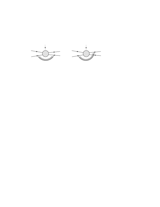
It is evident that the largest hard physical scale of the transition $B\to\pi$ is the heavy quark mass $m_{b}\sim M_{B}$. Therefore, the contribution of the hard region is somehow or other associated with the heavy quark decay. However, the hard-collinear scale $2E\omega$ implies participation of the light spectator with the momentum $k^{\mu}\sim\Lambda_{\mathrm{QCD}}$ in the process. Consequently, there are two subprocesses: the hard decay of the heavy quark into two partons that have $v$ and $\bar{v}$ fractions of the collinear momentum $q$, and semihard scattering of these partons by the soft spectator with the pion in final state (see Figure 5). To illustrate the general idea we consider an example of a radiative correction to the diagram Fig. 3. Namely, consider the two-loop correction shown in Figure 5 where the dash lines contour the subprocesses involved. In the case when the momentum $l_{1}$ is hard and $l_{2}$ is hard-collinear it is easy to calculate the contribution of this diagram sequentially in three steps: the first step is integration over the hard momentum $l_{1}$. In this step the virtualities of the quark and gluon produced in the heavy quark decay can be neglected, i.e., the momenta of the partons can be considered to be collinear to $n$:

$$\left(q-l_{2}\right)^{\mu}\sim\left(l_{2}-k\right)^{\mu}\sim(\lambda^{2},\lambda,1)\Rightarrow\left\{\begin{array}[c]{c}\left(l_{2}-k\right)^{\mu}\approx v\leavevmode\nobreak\ q^{\mu}\\ \left(q-l_{2}\right)^{\mu}\approx\bar{v}\leavevmode\nobreak\ q^{\mu}\end{array}\right.\,,$$ (30)

where $v=l_{2}\cdot n_{+}/(2E)$ is a dimensionless Sudakov parameter and $\bar{v}=1-v$. This part contains logarithms of the hard scale $\ln m_{b}/\mu$, we call it hard Wilson coefficient $C$ (hard coefficient function)

$$C\left(v,\ln\frac{m_{b}}{\mu},\frac{E}{m_{b}},\alpha_{s}\right)=\left\langle g(vq),q(\bar{v}q)\left|\leavevmode\nobreak\ \bar{q}\not\!n\,b\leavevmode\nobreak\ \right|b(p-k)\right\rangle\,,$$ (31)

averaging over the spin and color states is performed in the same way as for the amplitude (9). The second step is integration with respect to the components of the momentum $l_{2}$ except $v$, i.e., over the components that do not appear in the hard loop. This part, the so-called jet function, contains the logarithms of the semihard scale $\ln 2E\omega/\mu^{2}$:

$$J\left(u,v,\ln\frac{2E\omega}{\mu^{2}},\alpha_{s}\right)=E^{2}\,\left\langle\bar{q}(-q_{2}),q(q_{1})|\,g(vq),q(\bar{v}q),\bar{q}(-k)\right\rangle\,.$$ (32)

The last step is a convolution of the hard Wilson coefficient and the function with respect to the Sudakov parameter $v$, this convolution is convergent, i.e., it does not produce ”big” logarithms:

$$T(u,\omega,\mu,m_{b},E)=\frac{1}{E^{2}}\int_{0}^{1}dv\leavevmode\nobreak\ C\left(v,\ln\frac{m_{b}}{\mu},\frac{E}{m_{b}},\alpha_{s}\right)\leavevmode\nobreak\ J\left(u,v,\ln\frac{2E\omega}{\mu^{2}},\alpha_{s}\right)\,.$$ (33)

In terms of effective theory the first step of our consideration corresponds to the matching of the vector current in full QCD onto the set of three-body operators of $\mathrm{SCET}_{\mathrm{I}}$ (integrating out of hard modes), the second step corresponds to matching of the operators of the intermediate effective theory $\mathrm{SCET}_{\mathrm{I}}$ onto four-quark operators of $\mathrm{SCET}_{\mathrm{II}}$.

This simple partonic picture is only valid in the physical light-cone gauge $A\cdot n_{+}=0$ because in this gauge only one transverse gluon connects $C$ to $J$ but in the Feynman gauge it is accompanied by longitudinal collinear gluons. To be more specific, in the light-cone gauge the hard-collinear gluon produced in the heavy quark decay has a polarization that is approximately transverse to the $(n,n_{+})$ plane (see Eq.17)

$$d_{\mu\nu}(l_{2}-k)=\delta^{\mu\nu}-\frac{(l_{2}-k)^{\mu}\leavevmode\nobreak\ n_{+}^{\nu}+(l_{2}-k)^{\nu}\leavevmode\nobreak\ n_{+}^{\mu}}{2\leavevmode\nobreak\ (l_{2}-k)\cdot n_{+}-i0}\approx d_{\perp}^{\mu\nu}\,.$$ (34)

It is consistent with the fact that in this gauge the intermediate operator of $\mathrm{SCET}_{\mathrm{I}}$ has the form (here we use notation of [6]):

$$O_{1}^{1}(s_{1},s_{2})=\bar{\xi}_{C}(s_{1})\not\!\!A_{\perp}(s_{2})\,h_{v}(0)\,.$$ (35)

As can be seen from the consideration of the diagram 1b, the tree-level hard Wilson coefficient and the jet-function are

$$C\left(v,\ln\frac{m_{b}}{\mu},\frac{E}{m_{b}},\alpha_{s}\right)=1\,,\qquad J\left(u,v,\ln\frac{2E\omega}{\mu^{2}},\alpha_{s}\right)=\frac{\alpha_{s}}{u\,\omega}\,\delta(u-v)\,.$$ (36)

The loop corrections to them are presented in the following Sections.

4 Loop corrections

Following are the contributions of the five regions. The contributions of each diagram in all the regions except for the hard-collinear one are presented in the Feynman gauge. The expressions for the hard-collinear region are given in the light-cone gauge. As noted above, the loop corrections are normalized to the tree-level amplitude (14).

One further comment is in order. We use the ”naive dimensional regularization” (NDR) scheme that corresponds to omitting $\gamma_{5}$ in the projection operators (10) and (11). It can easily be shown that this scheme (using the projection operators (10) and (11) and calculation of a trace in dimensional regularization, i.e., without recourse to the Fierz transformations) is identical to the scheme with the basis of the evanescent operators chosen in [10].

4.1 Hard region

(a)

(b)

(c)

(d)

(e)

(f)

Figure 6: Loop correction to the hard coefficent function

We start the discussion of loops with the hard region. As stated earlier, it is necessary to consider the diagrams of the heavy quark decay into the collinear quark and transverse gluon (see Fig. 6). The contribution of each diagram is the following:

$$C\left(u,z,\ln\frac{m_{b}}{\mu},\alpha_{s}\right)=1+\frac{\alpha_{s}}{4\pi}\>\delta C\left(u,z,\ln\frac{m_{b}}{\mu}\right)\,,$$ (37)

$$\delta C_{a} = \,\left(C_{F}-\frac{C_{A}}{2}\right)\,\left[-\left(2\ln^{2}\frac{z\,m_{b}}{\mu}+\frac{\pi^{2}}{12}+\frac{2z}{\bar{z}}\ln z+2\,\mathrm{Li}_{2}\left(\bar{z}\right)\right)\right.$$ (38)

$$-\frac{2}{u}\,\left(2\,\ln\bar{u}\,\left(\ln\,\frac{m_{b}}{\mu}+\ln z-1\right)+\ln^{2}\bar{u}+\mathrm{Li}_{2}\left(1-\bar{u}\,z\right)-\mathrm{Li}_{2}\left(\bar{z}\right)\right)$$

$$\left.+\frac{1}{u}\,\left(\frac{\ln z}{\bar{z}}-\frac{\ln\,\bar{u}z}{(1-\bar{u}\,z)}+\ln\bar{u}\right)\right],$$

$$\delta C_{b} = \,\left(-\frac{C_{A}}{2}\right)\,\left[2\ln^{2}\frac{zm_{b}}{\mu}+\frac{\pi^{2}}{12}+\frac{2\,z\,\ln z}{\bar{z}}+2\,\mathrm{Li}_{2}\left(\bar{z}\right)\right.$$ (39)

$$\left.-\frac{1}{\bar{u}}\,\left(\frac{\ln z}{\bar{z}}-\frac{\ln\,uz}{(1-u\,z)}-3\,\ln u\right)\right],$$

$$\delta C_{c} = \,C_{F}\,\left[-2\,\ln\frac{m_{b}}{\mu}-\frac{1+\bar{z}}{\bar{z}}\,\ln z+1\right]$$ (40)

$$\delta C_{d} = \,\left(C_{F}-\frac{C_{A}}{2}\right)\,\left[-\frac{1}{\bar{u}}\,\left(\frac{\ln z}{\bar{z}}-\frac{\ln\,uz}{(1-u\,z)}+\ln u\right)\right.$$ (41)

$$\left.-\frac{1}{u}\,\left(\frac{\ln z}{\bar{z}}-\frac{\ln\,\bar{u}z}{(1-\bar{u}\,z)}+\ln\bar{u}\right)\right],$$

$$\delta C_{e} = \,C_{F}\,\left[\frac{z}{\bar{z}\,(1-u\,z)}+\frac{1}{\bar{u}}\,\left(\frac{\ln z}{\bar{z}^{2}}-\frac{\ln\,uz}{(1-uz)^{2}}\right)+\frac{\ln u}{\bar{u}}\right],$$ (42)

$$\delta C_{f} = \,C_{F}\,\left[3\,\ln\frac{m_{b}}{\mu}-2\right].$$ (43)

Note that the expressions (38–43) are finite in the limits $u\rightarrow 0$ and $u\rightarrow 1$, it confirms the fact that no logarithms of $m_{b}/\mu$ or $2E\omega/\mu^{2}$ are generated by the convolution of the hard Wilson coefficient and jet function. The final result of the hard Wilson coefficient takes the form

$$\delta C = \,\left(C_{F}-\frac{C_{A}}{2}\right)\,\left[-\frac{2}{u}\,\left(2\,\ln\bar{u}\,\left(\ln\,\frac{m_{b}}{\mu}+\ln z-1\right)+\ln^{2}\bar{u}+\mathrm{Li}_{2}\left(1-\bar{u}\,z\right)-\mathrm{Li}_{2}\left(\bar{z}\right)\right)\right.$$ (44)

$$\left.-\frac{2}{\bar{u}}\,\left(\frac{\ln z}{\bar{z}}-\frac{\ln u\,z}{(1-u\,z)}-\ln u\right)\right]$$

$$+\,C_{F}\,\left(-2\ln^{2}\frac{z\,m_{b}}{\mu}-\frac{\pi^{2}}{12}+\ln\frac{m_{b}}{\mu}+\frac{2+z}{\bar{z}}\,\ln z-2\,\mathrm{Li}_{2}\left(\bar{z}\right)-1+\frac{z}{\bar{z}\,(1-u\,z)}\right.$$

$$\left.+\frac{1}{\bar{u}}\,\left(\frac{\ln z}{\bar{z}^{2}}-\frac{\ln u\,z}{(1-u\,z)^{2}}+\frac{\ln z}{\bar{z}}-\frac{\ln u\,z}{(1-u\,z)}-2\,\ln u\right)\right).$$

As already mentioned, this result is a special case of the Wilson coefficient of the QCD vector current matched onto the corresponding three-body $\mathrm{SCET}_{\mathrm{I}}$ operator. Our result coincides with the result calculated in [7] and the corresponding combination of matching coefficients calculated in [11] where an operator basis different from [7] is used.

4.2 Hard-collinear region

Figure 7:

To calculate the contributions to the jet function, it is necessary to consider all diagrams of the scattering of the hard-collinear quark and gluon by the soft spectator.

In the diagram depicted in Fig. 7 we label the external lines by (1), (2), (4), (5) and the internal propagators by (3) and (6). The contributions to the corrections to the jet function can be generated by diagrams in which a gluon is attached to two labelled lines. We denote the contribution of each diagram by the letter $J$ with $\{ij\}$ subscript where $i$ and $j$ are the numbers of positions in Figure 7.

As emphasized above, loop corrections to the jet function have to be calculated in the light-cone gauge. In this gauge the contributions of the diagrams $\{4j\}$, where the gluon is radiated by the heavy quark, vanishes. The reason is that the heavy quark can radiate longitudinally polarized collinear gluons only; the contribution of these gluons is excluded by the condition $A\cdot n_{+}=0$. Diagrams $\{11\}$, $\{22\}$, $\{55\}$ do not contribute also because they do not contain the hard-collinear scale. Nonzero contributions are given by the following diagrams:

$$J_{\{15\}} =\left(C_{F}-\frac{C_{A}}{2}\right)\,\delta(v-u)\left(-\ln^{2}\frac{2E\omega}{\mu^{2}}+(3-2\,\ln u)\ln\frac{2E\omega}{\mu^{2}}\right.$$

$$\qquad\left.+3\,\ln u-{\ln}^{2}{u}-8+\frac{{\pi}^{2}}{6}\right),$$ (45)

$$J_{\{66\}} =C_{A}\,\delta(v-u)\left(2\ln^{2}\frac{2E\omega}{\mu^{2}}-\left(\frac{11}{3}-4\,\ln u\right)\ln\frac{2E\omega}{\mu^{2}}-\frac{11\,\ln u}{3}\right.$$

$$\qquad\left.+2\,{\ln}^{2}{u}+\frac{67}{9}-\frac{{\pi}^{2}}{3}\right)+T_{F}\,n_{f}\delta(v-u)\left(\frac{4}{3}\,\ln\frac{2E\omega}{\mu^{2}}+\frac{4}{3}\,\ln u-\frac{20}{9}\right),$$ (46)

$$J_{\{16\}} =\frac{C_{A}}{2}\,\delta(v-u)\left(-3\ln^{2}\frac{2E\omega}{\mu^{2}}+\left(3-6\,\ln u\right)\ln\frac{2E\omega}{\mu^{2}}\right.$$

$$\qquad\left.+3\,\ln u-3\,{\ln}^{2}{u}-6+\frac{{\pi}^{2}}{2}\right)\,,$$ (47)

$$J_{\{33\}} =2C_{F}\leavevmode\nobreak\ \bar{v}\,\left(\ln\frac{2E\omega}{\mu^{2}}+\ln(v\,\bar{v})+1\right)\,,$$ (48)

$$J_{\{23\}} =2\leavevmode\nobreak\ \left(C_{F}-\frac{C_{A}}{2}\right)\,\left(\theta(v-\bar{u})\leavevmode\nobreak\ \left(\,\frac{\,\bar{v}\leavevmode\nobreak\ \left(v-\bar{u}\right)}{v\,u}\left(\ln\frac{2E\omega}{\mu^{2}}+\ln(\bar{v})\right)\,\right.\right.$$

$$\left.+\,\frac{\left(v-\bar{u}\right)}{\bar{u}}\ln v-\frac{\,\left(v-\bar{u}\right)^{2}}{v\,u\,\bar{u}}\ \ln\left(1-\frac{\bar{v}}{u}\right)\,+\frac{\bar{v}}{v\,u}\right)$$

$$\left.+\,\theta(\bar{u}-v)\leavevmode\nobreak\ \frac{\bar{u}-v}{\bar{u}}\,\left(\frac{1}{\epsilon}-\ln v\bar{v}\right)\,\right)\,.$$ (49)

$$J_{\{25\}}+J_{\{26\}}+J_{\{12\}}=\left(C_{F}-\frac{C_{A}}{2}\right)$$

$$\times\,2\,\left[\frac{\theta(v-u)}{v-u}\,\left(\ln\frac{2E\omega}{\mu^{2}}+\ln(v-u)\right)+\frac{\theta(u-v)}{u-v}\,\left(\ln\frac{2E\omega}{\mu^{2}}+\ln(u-v)\right)\,\right]_{+}$$

$$+\left(C_{F}-\frac{C_{A}}{2}\right)\,\delta(v-u)\,2\,\left(\ln^{2}\frac{2E\omega}{\mu^{2}}+\ln(u\bar{u})\,\ln\frac{2E\omega}{\mu^{2}}+\frac{{\ln}^{2}{\bar{u}}}{2}+\frac{{\ln}^{2}{u}}{2}+\frac{{\pi}^{2}}{6}\right)$$

$$+C_{F}\,\theta(u-v)\,\frac{2\bar{v}}{\bar{u}\,u}\,\left(\ln\frac{2E\omega}{\mu^{2}}+\ln\left(\frac{v\,\left(u-v\right)}{u}\right)-\frac{\bar{u}}{\bar{v}}\right)$$

$$-\left(C_{F}-\frac{C_{A}}{2}\right)\,\frac{2\,\theta(u-v)}{u}\left(\frac{\bar{u}-v}{\bar{u}}\ln\frac{2E\omega}{\mu^{2}}-\frac{u}{u-v}\ln\frac{v}{u}+\frac{\left(\bar{u}-v\right)}{\bar{u}}\,\ln\frac{v\,\left(u-v\right)}{u}-1\right)$$

$$+\left({C_{F}-}\frac{{C_{A}}}{2}\right)\,\frac{2\,\theta(v-u)}{v}\left(-\ln\frac{2E\omega}{\mu^{2}}+\frac{u}{v-u}\ln\frac{\bar{v}}{\bar{u}}-\ln(v-u)+\frac{\bar{v}}{\bar{u}}\right)\,$$

$$+\left({C_{F}-}\frac{C_{A}}{2}\right)\,\frac{2\,\left(\bar{u}-v\right)}{\bar{u}}\,\,\left(\ln\frac{2E\omega}{\mu^{2}}+\ln v\bar{v}\right)\,$$

$$-{C_{F}\,}\frac{2\,\bar{v}\,}{\bar{u}}\left(\ln\frac{2E\omega}{\mu^{2}}+\ln v\bar{v}-\frac{\bar{u}}{\bar{v}}\right)-2\,{C_{F}}\,\frac{\,\theta(v-u)}{v}\,.$$ (50)

As in the case of the hard coefficient function, the corrections to the jet function are finite in the $u\to 0$ limit. It in particular means that the corresponding convolution integral with pion light-cone distribution amplitude is convergent. The final result for the jet functions has the form:

$$J\left(u,v,\ln\frac{2E\omega}{\mu^{2}},\alpha_{s}(\mu)\right)=\frac{\alpha_{s}}{u\,\omega}\left(\delta(u-v)\right.\\ \left.+\frac{\alpha_{s}}{4\pi}\leavevmode\nobreak\ \left(C_{F}\leavevmode\nobreak\ \ln^{2}\frac{2E\omega}{\mu^{2}}\leavevmode\nobreak\ \delta(u-v)+j_{1}(u,v)\leavevmode\nobreak\ \ln\frac{2E\omega}{\mu^{2}}+j_{2}(u,v)\right)\right)\,,$$ (51)

where functions $j_{1}(u,v)$ $j_{2}(u,v)$ are defined by

$$j_{1}(u,v) =\delta(v-u)\leavevmode\nobreak\ \left(-\frac{C_{A}}{2}\leavevmode\nobreak\ \left(\frac{13}{3}-2\ln u\right)+\left(C_{F}-\frac{C_{A}}{2}\right)\leavevmode\nobreak\ \left(3+2\ln\bar{u}\right)+\frac{4}{3}\,T_{F}\,n_{f}\right)$$

$$-\left(\frac{{C_{A}}}{2}-{C_{F}}\right)\leavevmode\nobreak\ 2\,\left[\frac{\theta(v-u)}{v-u}\,+\frac{\theta(u-v)}{u-v}\right]_{+}$$

$$+\left(C_{F}-\frac{C_{A}}{2}\right)\,\frac{2\leavevmode\nobreak\ \left(v-\bar{u}\right)}{\bar{u}}\left(\theta(v-\bar{u})\leavevmode\nobreak\ \frac{\bar{v}\leavevmode\nobreak\ \bar{u}}{v\,u}+\,\theta(\bar{u}-v)\leavevmode\nobreak\ \,\right)$$

$$-\left(C_{F}-\frac{C_{A}}{2}\right)\,\,2\left(\leavevmode\nobreak\ \theta(u-v)\leavevmode\nobreak\ \frac{\bar{u}-v}{u\bar{u}}+\theta(v-u)\leavevmode\nobreak\ \frac{1\,}{v}-\frac{\bar{u}-v}{\bar{u}}\,\right)$$

$$+{C_{F}\leavevmode\nobreak\ 2}\left(-\frac{u\,\bar{v}\,}{\bar{u}}+\leavevmode\nobreak\ \theta(u-v)\,\frac{\bar{v}}{\bar{u}\,u}\,\,\right)\,,$$ (52)

$$j_{2}(u,v) =\delta(v-u)\left(\frac{C_{A}}{2}\left(\frac{80}{9}-\frac{\pi^{2}}{6}-\frac{13}{3}\ln u+\ln^{2}u\right)-T_{F}\,n_{f}\left(\frac{20}{9}-\frac{4}{3}\,\ln u\right)\right.$$

$$\left.+\left(C_{F}-\frac{C_{A}}{2}\right)\left(-8+\frac{\pi^{2}}{2}+\ln^{2}\bar{u}+3\ln u\right)\right)$$

$$+\left({C_{F}}-\frac{{C_{A}}}{2}\right)\leavevmode\nobreak\ 2\,\left[\frac{\theta(v-u)}{v-u}\,\ln(v-u)+\frac{\theta(u-v)}{u-v}\,\ln(u-v)\,\right]_{+}$$

$$-2\,{C_{F}}\leavevmode\nobreak\ \left(\frac{\,\theta(v-u)}{v}+\frac{\theta(u-v)}{u}\right)$$

$$+\left(C_{F}-\frac{C_{A}}{2}\right)\,\,\theta(u-v)\leavevmode\nobreak\ \frac{2}{u}\left(\frac{v}{u-v}\ln\frac{v}{u}-\ln\left(u-v\right)+1\right)$$

$$+\left({C_{F}-}\frac{{C_{A}}}{2}\right)\leavevmode\nobreak\ \theta(v-u)\leavevmode\nobreak\ \frac{2\,}{v}\left(\frac{u}{v-u}\ln\frac{\bar{v}}{\bar{u}}-\ln(v-u)+\frac{\bar{v}}{\bar{u}}\right)\,$$

$$+\left(C_{F}-\frac{C_{A}}{2}\right)\,\frac{2}{vu}\leavevmode\nobreak\ \theta(v-\bar{u})\leavevmode\nobreak\ \left(\bar{v}-\frac{\,\left(v-\bar{u}\right)^{2}}{\bar{u}}\ \ln\frac{\bar{v}\leavevmode\nobreak\ \left(u-\bar{v}\right)}{u}\right)\,\,$$

$$+{C_{F}\leavevmode\nobreak\ 2}\left(1+{\bar{v}}-\frac{{\bar{v}}u\,}{\bar{u}}\ln v\bar{v}\right)+2\leavevmode\nobreak\ \frac{\theta(u-v)}{u\bar{u}}\ln\frac{v\,\left(u-v\right)}{u}\left(C_{F}\leavevmode\nobreak\ -\frac{C_{A}}{2}\,\,v\right)\,.$$ (53)

The result obtained is in complete agreement with the result calculated in [7] (In our notations the corresponding correction is $-j_{\|}(\bar{u},\bar{v})$, where $j_{\|}$ is the function derived in [7])

4.3 Collinear region

Figure 8:

Figure 9:

Figure 10:

In this Section we consider factorization of the collinear singularities, i.e., the singularities associated with the radiation of a collinear gluon (momentum scaling is $(\lambda^{4},\lambda^{2},1))$. Such singularities have an origin in the singularity of a collinear quark propagator when a gluon is radiated in the direction of the quark. These singularities can be regularized by introduction of the soft transverse momentum (see (19), (20)). The logarithms that result are $\ln\mu^{2}/\mathbf{q}^{2}_{\perp}$, where $\mu$ is a factorization scale. As we shall see later, all collinear divergencies correspond to the renormalization of the pion LCDA. Thus, these singularities are cancelled by the substraction of the loop corrections corresponding to renormalization of the LCDA from the total loop corrections:

$$\Delta f =\Phi^{+}(\omega)\otimes T_{0}(\omega,u^{\prime})\otimes\delta\phi_{\pi}(u^{\prime})$$ (54)

$$\delta\phi_{\pi}(u^{\prime},\mu) =\frac{g^{2}}{(4\pi)^{2}}\,C_{F}\,\ln\frac{\mu^{2}}{\mathbf{q}_{\perp}^{2}}\>V^{(1)}_{\pi}(u^{\prime},u)\otimes\phi_{\pi}(u,\mu)\,,$$ (55)

where $V^{(1)}_{\pi}(u^{\prime},u)$ is ERBL kernel [12], [13],

$$\left\langle\pi(q)\left|\,\bar{q}_{\alpha}(sn_{+})W\left(sn_{+},0\right)q_{\beta}(0)\right|0\right\rangle=\frac{if_{\pi}}{4}\left(n_{+}\cdot q\right)\leavevmode\nobreak\ \left[\frac{\not\!n}{2}\gamma_{5}\right]_{\beta\alpha}\int_{0}^{1}du\,e^{ius\left(n_{+}\cdot q\right)}\phi_{\pi}(u)\,.$$ (56)

The contribution of each diagram for both the collinear and soft regions is denoted by

$$\Delta f=-K_{\pi}\,K_{B}\,C_{F}\,N_{c}\,(D-2)\,\frac{g^{2}}{E^{2}}\int_{0}^{1}\frac{du}{u}\int_{0}^{\infty}\frac{d\omega}{\omega}\,\Phi_{+}(\omega)A_{\{ij\}}(\omega,u)\phi_{\pi}(u)\,,$$ (57)

where $i$ and $j$ are the numbers of positions in the Figure 7 for the collinear gluon emission and absorbtion (see also definitions for the tree-level amplitude (14)).

First of all, we consider the contributions of the diagrams where the light antiquark radiates the collinear gluon, i.e., the $\{1i\}$ diagrams. Using the following notation for the amplitudes $A_{\{1i\}}$

$$A_{\{1i\}}=2i\,g^{2}\int[dl]\,\frac{\tilde{A}_{\{1i\}}}{\left(l^{2}+i0\right)\left((q_{1}-l)^{2}+i0\right)}\,,$$ (58)

we find the following integrands

$$\tilde{A}_{\{15\}} =\left(C_{F}-\frac{C_{A}}{2}\right)\left(-1+\frac{u}{\beta}\right), \tilde{A}_{\{16\}} =-\frac{C_{A}}{2}\,,$$ (59)

$$\tilde{A}_{\{14\}} =\left(C_{F}-\frac{C_{A}}{2}\right)\left(-\frac{u}{\beta}+\frac{u}{\beta-1}\right), \tilde{A}_{\{13\}} =\left(C_{F}-\frac{C_{A}}{2}\right)\left(-\frac{u}{\beta-1}\right)\,,$$ (60)

where $\beta=(l\cdot n_{+})/2E$ is a dimensionless Sudakov parameter. The corresponding corrections to the pion LCDA is depicted in Figure 10. The dash line denotes the Wilson line $W\left(sn_{+},0\right)$ which is connecting the quark fields in the LCDA. The sum of the contributions of the {1i} diagrams is cancelled by the correction convoluted with the tree-level coefficient function $1/u$:

$$\int_{0}^{1}\frac{du}{u}\,\phi_{\pi}(u)\sum_{i}A_{\{1i\}}(u)\rightarrow\int_{0}^{1}\frac{du^{\prime}}{u^{\prime}}\int_{0}^{1}du\leavevmode\nobreak\ V_{\ref{f_LA1}}(u^{\prime},u)\leavevmode\nobreak\ \phi_{\pi}(u)$$ (61)

$$=-2ig^{2}C_{F}\int_{0}^{1}\frac{du^{\prime}}{u^{\prime}}\int_{0}^{1}\phi_{\pi}(u)\leavevmode\nobreak\ du\int[dl]\leavevmode\nobreak\ \frac{\leavevmode\nobreak\ \beta-u}{\left((l-q_{1})^{2}+i0\right)\left(l^{2}+i0\right)}\leavevmode\nobreak\ \frac{\delta(u^{\prime}-u)-\delta\left(u^{\prime}-(u-\beta)\right)}{\beta+i0}$$

$$=-2ig^{2}\int_{0}^{1}\frac{\phi_{\pi}(u)}{u}\leavevmode\nobreak\ du\int[dl]\leavevmode\nobreak\ \frac{C_{F}}{\left((l-q_{1})^{2}+i0\right)\left(l^{2}+i0\right)}\,.$$ (62)

The collinear singularities corresponding to the radiation of the collinear gluon by the light quark (the {2i} diagrams) can be considered in a similar manner:

$$A_{\{2i\}}=2i\,g^{2}\int[dl]\,\frac{\tilde{A}_{\{2i\}}}{\left(l^{2}+i0\right)\left((q_{2}-l)^{2}+i0\right)}\,,$$ (63)

$$\tilde{A}_{\{25\}} =\left(C_{F}-\frac{C_{A}}{2}\right)\left(\frac{\beta-\bar{u}}{\beta}-\frac{\beta-\bar{u}}{\beta+u}\right), \tilde{A}_{(26)} =-\frac{C_{A}}{2}\left(\frac{\beta-\bar{u}}{\beta+u}\right),$$ (64)

$$\tilde{A}_{\{24\}} =\left(C_{F}-\frac{C_{A}}{2}\right)\left(-\frac{\beta-\bar{u}}{\beta}+\frac{\beta-\bar{u}}{\beta-1}\right), \tilde{A}_{\{23\}} =\left(C_{F}-\frac{C_{A}}{2}\right)\left(-\frac{\beta-\bar{u}}{\beta-1}\right).$$ (65)

The sum of the contributions of these diagrams is cancelled by the correction depicted in Figure 10.

$$\int_{0}^{1}\frac{du}{u}\,\phi_{\pi}(u)\sum_{i}A_{\{2i\}}(u)\rightarrow\int_{0}^{1}\frac{du^{\prime}}{u^{\prime}}\int_{0}^{1}du\leavevmode\nobreak\ V_{\ref{f_LA2}}(u^{\prime},u)\leavevmode\nobreak\ \phi_{\pi}(u)$$ (66)

$$=2ig^{2}C_{F}\int_{0}^{1}\frac{du^{\prime}}{u^{\prime}}\int_{0}^{1}\phi(u)\leavevmode\nobreak\ du\int[dl]\leavevmode\nobreak\ \frac{\leavevmode\nobreak\ (\bar{u}-\beta)}{\left((l-q_{2})^{2}+i0\right)\left(l^{2}+i0\right)}\leavevmode\nobreak\ \frac{\left(\delta(u^{\prime}-u)-\delta\left(u^{\prime}-(u+\beta)\right)\right)}{\beta+i0}$$

$$=2ig^{2}\int_{0}^{1}\frac{\phi(u)}{u}\leavevmode\nobreak\ du\int[dl]\leavevmode\nobreak\ \frac{C_{F}}{\left((l-q_{2})^{2}+i0\right)\left(l^{2}+i0\right)}\leavevmode\nobreak\ \frac{\bar{u}-\beta}{u+\beta}\,.$$ (67)

The diagram {12} with the collinear gluon exchange between the quark and antiquark

$$A_{\{12\}}=-2ig^{2}\,C_{F}\,\int[dl]\frac{\left(\mathbf{l}_{\perp}-\mathbf{q}_{\perp}\right)^{2}}{\left(l^{2}+i0\right)\left((q_{1}-l)^{2}+i0\right)\left((q_{2}+l)^{2}+i0\right)}\frac{u}{\beta-u+i0}$$ (68)

is cancelled by the corresponding diagram Fig. 10. The self-energy diagrams $\{11\}$ and $\{22\}$ are trivially cancelled by the renormalization of the quark fields in the pion light-cone distribution amplitude.

4.4 Soft region

Figure 11:

Figure 12:

Figure 13:

Below is a consideration of the singularities associated with the soft region $l\sim(\lambda^{2},\lambda^{2},\lambda^{2})$. This region occurs in the diagrams with a gluon radiated by the slow-moving heavy quark or by the soft spectator. Assuming $p^{2}=m_{b}^{2}$, the singularities arise as logarithms $\ln\mu^{2}/\left|k^{2}\right|$. These ”big” logarithms are absorbed by the renormalization of the $B$-meson light-cone distribution amplitude:

$$\Delta f =\delta\Phi^{+}(\omega^{\prime})\otimes T_{0}(\omega^{\prime},u)\otimes\phi_{\pi}(u)$$ (69)

$$\delta\Phi^{+}(\omega^{\prime},\mu) =\frac{g^{2}}{(4\pi)^{2}}\,C_{F}\,\left(\Gamma^{(1)}\,\ln^{2}\frac{\mu^{2}}{\left|k^{2}\right|}\,\Phi^{+}(\omega^{\prime},\mu)+\ln\frac{\mu^{2}}{\left|k^{2}\right|}\,U^{(1)}(\omega^{\prime},\omega)\otimes\Phi^{+}(\omega,\mu)\right)\,,$$ (70)

where $\Gamma^{(1)}$ and $U^{(1)}(\omega^{\prime},\omega)$ are the functions contained in the kernel of the evolution equation [14], [15] of the corresponding B-meson light-cone distribution amplitude $\Phi^{+}(\omega)$ [16], [4]

$$\left\langle 0\left|\bar{q}_{\alpha}(sn)\leavevmode\nobreak\ W(sn,0)\leavevmode\nobreak\ h_{v\beta}(0)\right|\bar{B}(p)\right\rangle\\ =-\frac{if_{B}M_{B}}{4}\int_{0}^{\infty}d\omega\,e^{-i\omega s}\left(\frac{1+\not\!v}{2}\left[\left(n\cdot v\right)\not\!n_{+}\,\Phi_{+}(\omega)+\left(n_{+}\cdot v\right)\not\!n\,\Phi_{-}(\omega)\right]\gamma_{5}\right)_{\beta\alpha}\,.$$ (71)

First of all we consider the diagrams with a gluon radiated by the heavy quark. As in the case of the collinear region, we introduce the following notation:

$$A_{\{4i\}}=2i\,g^{2}\int[dl]\frac{m_{b}\leavevmode\nobreak\ \tilde{A}_{\{4i\}}}{\left(l^{2}+i0\right)\left((p-k-l)^{2}-m_{b}^{2}\right)}\,.$$ (72)

The integrands of the {4i} diagrams are as follows:

$$\tilde{A}_{\{42\}}=\left(C_{F}-\frac{C_{A}}{2}\right)\frac{1}{\alpha}\,,\quad\tilde{A}_{\{41\}}=\left(C_{F}-\frac{C_{A}}{2}\right)\left(\frac{1}{\alpha+\omega}-\frac{1}{\alpha}\right)\,,\quad\tilde{A}_{\{46\}}=\frac{C_{A}}{2}\frac{1}{\alpha+\omega}\,,$$ (73)

where $\alpha=(l\cdot n)$. Being convoluted with the tree-level coefficient function $1/\omega$ , the contribution to the LCDA’s renormalization (Fig.13) with gluon radiation by the heavy quark cancels the sum of the contributions of the {4i} diagrams

$$\int_{0}^{\infty}\frac{d\omega}{\omega}\,\Phi_{+}(\omega)\sum_{i}A_{\{4i\}}(\omega)\rightarrow\int_{0}^{\infty}\frac{d\omega^{\prime}}{\omega^{\prime}}\int_{0}^{\infty}d\omega\,V_{\ref{f_LB1}}(\omega^{\prime},\omega)\,\Phi_{+}(\omega)$$ (74)

$$=-ig^{2}C_{F}\int_{0}^{\infty}\frac{d\omega^{\prime}}{\omega^{\prime}}\int_{0}^{\infty}d\omega\int[dl]\,\frac{1}{\left((l+k)\cdot v-i0\right)\left(l^{2}+i0\right)}\,\frac{\delta(\omega^{\prime}-\omega)-\delta(\omega^{\prime}-\omega-\alpha)}{\alpha-i0}\,\Phi_{+}(\omega)$$

$$=-ig^{2}\int_{0}^{\infty}\frac{d\omega}{\omega}\,\Phi_{+}(\omega)\int[dl]\,\frac{C_{F}}{\left((l+k)\cdot v-i0\right)\left(l^{2}+i0\right)}\,\frac{1}{\omega+\alpha}\,.$$ (75)

The contributions of the diagrams with the gluon radiation by the soft spectator can be considered in a similar way

$$A_{\{5i\}}=-2i\,g^{2}\int[dl]\frac{\tilde{A}_{\{5i\}}}{\left((l-k)^{2}+i0\right)\left(l^{2}+i0\right)}\,,$$ (76)

$$\tilde{A}_{\{51\}}=\left(C_{F}-\frac{C_{A}}{2}\right)\frac{\alpha-\omega}{\alpha}\,,\quad\tilde{A}_{\{52\}}=\left(C_{F}-\frac{C_{A}}{2}\right)\frac{\omega}{\alpha}\,,\quad\tilde{A}_{\{56\}}=\frac{C_{A}}{2}\,.$$ (77)

The sum of the contributions is cancelled by the contribution to the LCDA’s renormalization (Fig. 13) with radiation of a gluon by the soft spectator

$$\int_{0}^{\infty}\frac{d\omega}{\omega}\,\Phi_{+}(\omega)\sum_{i}A_{\{5i\}}(\omega)\rightarrow\int_{0}^{\infty}\frac{d\omega^{\prime}}{\omega^{\prime}}\int_{0}^{\infty}d\omega\leavevmode\nobreak\ V_{\ref{f_LB2}}(\omega^{\prime},\omega)\leavevmode\nobreak\ \Phi_{+}(\omega)$$ (78)

$$=-2ig^{2}C_{F}\int_{0}^{\infty}\frac{d\omega^{\prime}}{\omega^{\prime}}\int_{0}^{\infty}d\omega\int[dl]\,\frac{(\alpha-\omega)}{\left((l-k)^{2}+i0\right)\left(l^{2}+i0\right)}\,\frac{\delta(\omega^{\prime}-\omega)-\delta(\omega^{\prime}-(\omega-\alpha))}{\alpha-i0}\,\Phi_{+}(\omega)$$

$$=-2ig^{2}\int_{0}^{\infty}\frac{d\omega}{\omega}\,\Phi_{+}(\omega)\int[dl]\,\frac{C_{F}}{\left((l-k)^{2}+i0\right)\left(l^{2}+i0\right)}\,.$$ (79)

The situation with the diagrams $\{44\}$ and $\{55\}$ is similar to the one in the collinear region, these diagrams correspond to the renormalization of the quark field in the light-cone distribution amplitude of the $B$-meson. The soft region of the diagram $\{45\}$ is power suppressed; it exactly corresponds to the absence of the contribution to the evolution kernel from the diagram Fig. 13.

4.5 Soft-collinear

In this Section we consider the contribution of the soft-collinear region, i.e., the region where the momentum of a gluon has its’ components $\displaystyle l=\left((l\cdot n),l_{\perp},(l\cdot n_{+})\right)$ that are of order $(\lambda^{4},\lambda^{3},\lambda^{2})$.

According to the idea of the method of expanding by regions, for the difference of the form factors to be independent on the intermediate factorization scale, it is necessary to sum the contributions of all the regions, the soft-collinear region included. However, the contribution of this region does not correspond to the summation of the leading logarithms for any of the objects in the expression (7), therefore, it has to be cancelled in the sum of the diagrams by itself. This cancellation corresponds to the idea that, in the framework of the effective theory, after integration out of the hard and hard-collinear modes the soft and collinear degrees of freedom should be decoupled from one another. At this specified condition, a matrix element, containing the soft and collinear modes, can be factorized into matrix elements of ”soft” and of ”collinear” operators separately. This is of critical importance for a derivation of a factorization formula of type (7). We show the cancellation of soft-collinear region contributions for pion final state, though it is liable to brake down in general case [17].

Figure 14:

The cancellation of the contribution of the soft-collinear region occurs in line with the idea of color transparency [18], which is underlying the factorization approach to exclusive processes: the final state hadron produced by hard scattering is a color singlet state. Thus, there is a rather weak (dipole) interaction with gluons, the wavelength of which is larger than the size of the hadron. Therefore, it is hoped that there is a cancellation of the soft logarithmic singularities of the radiative corrections between graphs in which the soft gluon couples to a parton in the initial state and different constituents of the final state (see Fig. 14). Whereas the remaining infrared singularities factorize into the LCDAs of each hadron separately.

To calculate loop corrections it is convenient to introduce the followng dimensionless variables:

$$(l\cdot n_{+})\rightarrow\frac{\left|k^{2}\right|}{\omega}\leavevmode\nobreak\ \beta,\leavevmode\nobreak\ (l\cdot n)\rightarrow\frac{\mathbf{q}_{\perp}^{2}}{2E}\leavevmode\nobreak\ \alpha,\leavevmode\nobreak\ \mathbf{l}_{\perp}^{2}\rightarrow\frac{\left|k^{2}\right|\mathbf{q}_{\perp}^{2}}{2E\omega}\leavevmode\nobreak\ \mathbf{l}_{\perp}^{2}.$$

The contribution of the diagram {25} with these variables takes the form:

$$\{25\}=i\,g^{2}\left(C_{F}-\frac{C_{A}}{2}\right)\left(\frac{\mu^{2}2E\omega}{\left|k^{2}\right|\mathbf{q}_{\perp}^{2}}\right)^{\epsilon}\int[dl]\leavevmode\nobreak\ \frac{2\bar{u}}{\left(l^{2}+i0\right)(\beta-1+i0)(\alpha\bar{u}-1+i0)}.$$ (80)

After the additional substitution $\alpha\to\alpha/\bar{u},l_{\perp}\to l_{\perp}/\bar{u}^{1/2}$ we find

$$\{25\} =i\,g^{2}\left(C_{F}-\frac{C_{A}}{2}\right)\left(\frac{\mu^{2}2E\omega}{\left|k^{2}\right|\mathbf{q}_{\perp}^{2}}\right)^{\epsilon}\int[dl]\leavevmode\nobreak\ \frac{2\bar{u}^{\epsilon}}{\left(l^{2}+i0\right)(\beta-1+i0)(\alpha-1+i0)}\,.$$ (81)

The final result of the integral is the expression (26). The similar expression for the diagram {15} is

$$\{15\}=-i\,g^{2}\left(C_{F}-\frac{C_{A}}{2}\right)\left(\frac{\mu^{2}2E\omega}{\left|k^{2}\right|\mathbf{q}_{\perp}^{2}}\right)^{\epsilon}\int[dl]\leavevmode\nobreak\ \frac{2u^{\epsilon}}{\left(l^{2}+i0\right)(\beta-1+i0)(\alpha-1+i0)}\,.$$ (82)

Contrary to our expectations, the expressions (81) and (82) are not only of opposite sign, but they also differ by the factors $u^{\epsilon}$ and $\bar{u}^{\epsilon}$. It immediately follows that in the case of the partons with $u$ and $\bar{u}$ fractions of the longitudinal momentum there is a cancellation of double Sudakov logarithms only, but not of single ones. However, the pion LCDA is symmetric with a substitution $u\leftrightarrow\bar{u}$ while the sum of the expressions (81) and (82) is antisymmetric. Therefore, being averaged over the pion light-cone distribution amplitude, the contribution of the soft-collinear region vanishes.

The diagrams {14} and {24} can be considered in a similar manner:

$$\{14\} =-i\,g^{2}\left(C_{F}-\frac{C_{A}}{2}\right)\left(\frac{\mu^{2}2E\omega}{\left|k^{2}\right|\mathbf{q}_{\perp}^{2}}\right)^{\epsilon}\int[dl]\leavevmode\nobreak\ \frac{2u\leavevmode\nobreak\ \left|k^{2}\right|}{l^{2}(1+\alpha u)\left(\left|k^{2}\right|\bar{\beta}-\omega^{2}\right)}\,,$$ (83)

$$\{24\} =i\,g^{2}\left(C_{F}-\frac{C_{A}}{2}\right)\left(\frac{\mu^{2}2E\omega}{\left|k^{2}\right|\mathbf{q}_{\perp}^{2}}\right)^{\epsilon}\int[dl]\leavevmode\nobreak\ \frac{2\bar{u}\leavevmode\nobreak\ \left|k^{2}\right|}{l^{2}(1+\alpha\bar{u})\left(\left|k^{2}\right|\bar{\beta}-\omega^{2}\right)}\,.$$ (84)

Even before the integration one can see that the sum of the expressions (83), (84) is antisymmetric with respect to the substitution $u\leftrightarrow\bar{u}$. Hence, it vanishes in the convolution with the pion light cone-distribution amplitude.

5 Conclusion

The semileptonic decay $B\to\pi l\nu$ has been discussed in this article. It is known that at a large energy of recoil to the lepton pair there is the relation of the form factors that parametrize an amplitude of this decay. This relation can be violated by the hard and semihard radiative corrections. In this paper we have studied the factorizable contribution of these corrections. In particular, loop corrections to the hard Wilson coefficient and to the jet function have been calculated. In contrast to the soft-collinear effective theory, to calculate loop corrections we have used the method of expanding by regions. The corrections obtained are in complete agreement with previous results of Beneke, Kiyo and Yang [11] and results of Hill, Becher, Lee and Neubert [7]. The factorization of the soft and collinear singularities has been shown at one-loop level. We have demonstrated the cancellation of the contribution of the soft-collinear modes by taking into account the symmetry of the pion light-cone distribution amplitude; this fact is of critical importance to the factorization approach to this decay.

Note added. After I completed this paper, the results of M. Beneke and D. Yang mentioned above have appeared in preprint [19].

I would like to thank N. Kivel for his helpful comments and discussions and M. Beneke for pointing out the dependence of the one-loop jet function on the choice of evanescent operators. The investigation was supported by the Russian Foundation for Basic Research through Grant No. 05-02-16627-a and by Institut $\mathrm{f\ddot{u}r}$ Theoretische Physik-II Ruhr-$\mathrm{Universit\ddot{a}t}$ through
Graduiertenkolleg ”Physik der Elementarteilchen an Beschleunigern und im Universum”.

References

- [1] C. W. Bauer, S. Fleming, D. Pirjol and I. W. Stewart, Phys. Rev. D 63 (2001) 114020 [hep-ph/0011336].
- [2] M. Beneke, A. P. Chapovsky, M. Diehl and T. Feldmann, Nucl. Phys. B 643 (2002) 431 [hep-ph/0206152].
- [3] J. Charles et al., Phys. Rev. D 60 (1999) 014001 [hep-ph/9812358].
- [4] M. Beneke, T. Feldmann, Nucl. Phys. B 592 (2001) 3 [hep-ph/0008255].
- [5] C. W. Bauer, D. Pirjol, I. W. Stewart, Phys. Rev. D 67 (2003) 071502 [hep-ph/0211069].
- [6] M. Beneke, T. Feldmann, Nucl. Phys. B 685 (2004) 249 [hep-ph/0311335].
- [7] R. J. Hill, T. Becher, S. J. Lee, M. Neubert, JHEP 0407 (2004) 081 [hep-ph/0404217].
-
[8]
V. A. Smirnov, E. R. Rakhmetov, Theor. Math. Phys.
120 (1999) 870 [Theor. Mat. Fiz. 120 (1999) 64]
[hep-ph/9812529].
V. A. Smirnov, Applied Asymptotic Expansions In Momenta And Masses, Springer Verlag, Berlin, Germany, 2002. - [9] S. Descotes-Genon, C. T. Sachrajda, Nucl. Phys. B 693 (2004) 103 [hep-ph/0403277].
- [10] T. Becher, R. J. Hill, [hep-ph/0408344].
- [11] M. Beneke, Y. Kiyo, D. S. Yang, Nucl. Phys. B 692 (2004) 232 [hep-ph/0402241].
- [12] A. V. Efremov and A. V. Radyuskin, Phys. Rev. D 21 (1980) 245.
- [13] G. P. Lepage and S. J. Brodsky, Phys. Rev. D 22 (1980) 2157.
- [14] S. W. Bosh, R. J. Hill, B. O. Lange and M. Neubert, Phys. Rev. D 67 (2003) 094014 [hep-ph/0301123].
- [15] B. O. Lange and M. Neubert, Phys. Rev. Lett. 91 (2003) 102001 [hep-ph/0303082].
- [16] A. G. Grozin and M. Neubert, Phys. Rev. D 55 (1997) 272 [hep-ph/9607366].
- [17] T. Becher, R. J. Hill, M. Neubert, Phys. Rev. D 69 (2004) 054017 [hep-ph/0308122].
- [18] J. D. Bjorken, Nucl. Phys. Proc. Suppl. 11 (1989) 325.
- [19] M. Beneke, D. Yang, [hep-ph/0508250].