Continuum physics
with quenched overlap fermions

Abstract

We calculate $m_{ud}\!=\!(m_{u}\!+\!m_{d})/2$, $m_{s}$, $f_{\pi}$ and $f_{K}$ in the quenched continuum limit with UV-filtered overlap fermions. We see rather small scaling violations on lattices as coarse as $a^{-1}\!\simeq\!1\,\mathrm{GeV}$ and conjecture that similar advantages would be manifest in unquenched studies.

1 Introduction

Overlap fermions [2] satisfy the Ginsparg-Wilson relation [3]

$${\gamma_{5}}D+D\hat{\gamma_{5}}=0\;,\qquad\hat{\gamma_{5}}={\gamma_{5}}(1-{1\over\rho}D)$$ (1)

which implies exact chiral symmetry at finite lattice spacing [4, 5]. While theoretically clean, calculations with overlap fermions are considered a computational challenge. In a recent investigation [6] it has been conjectured that a UV-filtered (smeared) Wilson kernel operator, as previously suggested in [7, 8, 9, 10], might substantially reduce the computational cost associated with obtaining continuum physics [11]. In [6] the focus was on technical aspects, but it is clear that the point relevant in practical applications is whether UV-filtered (“thick link”) overlap fermions would extend the scaling region to significantly coarser lattices, even if one refrains from ($\beta$-specific) tuning and sets $\rho\!=\!1$. The present note addresses this question by studying the continuum limit of the pseudoscalar masses and decay constants with quenched UV-filtered overlap quarks. No systematic comparison to plain (“thin link”) overlap fermions is made, because we could not obtain reasonable signals for plain overlap fermions with $\rho\!=\!1$ on our coarser lattices. Given the exploratory nature of the present investigation, we restrict ourselves to pseudoscalar meson correlators in the $p$-regime of Chiral Perturbation Theory (XPT) [12]. Our main results are the values of the quenched strange quark mass and $K$ decay constant in the continuum

$$m_{s}(\overline{\mathrm{MS}},2\,\mathrm{GeV})=119(10)(7)\,\mathrm{MeV}\;,\qquad f_{K}=170(10)(2)\,\mathrm{MeV}$$ (2)

as well as the quark mass and decay constant ratios

$${m_{s}\over m_{ud}}=23.3(7.1)(4.5)\;,\qquad{f_{K}/f_{\pi}}=1.17(4)(2)$$ (3)

where $m_{ud}\!=\!(m_{u}\!+\!m_{d})/2$ and no numerical input from XPT has been used. Throughout this note the first error is statistical and the second systematic, but the latter does not include any estimate of the quenching effect.

2 Technical setup

We use the Wilson gauge action. The massless overlap operator is [2]

$$D_{\mathrm{ov}}=\rho\Big{[}1+(D_{\mathrm{W}}-\rho)\big{(}(D^{\dagger}_{\mathrm{W}}-\rho)(D_{\mathrm{W}}-\rho)\big{)}^{-1/2}\Big{]}$$ (4)

with $D_{\mathrm{W}}$ the massless Wilson operator. The UV-filtered overlap is constructed by evaluating the Wilson operator on APE [13] or HYP [14, 15] smeared gauge configurations, resulting in an $O(a^{2})$ redefinition of the fermion action [16, 6]. We use 1 or 3 iterations with smearing parameters $\alpha_{\mathrm{APE}}\!=\!0.5$ or $\alpha_{\mathrm{HYP}}\!=\!(0.75,0.6,0.3)$ and the shift parameter $\rho\!=\!1$ is kept fixed. Based on (4) the massive operator is defined through

$$D_{\mathrm{ov},m}=\Big{(}1-{am\over 2\rho}\Big{)}D_{\mathrm{ov}}+m\;.$$ (5)

We set the lattice spacing with the Sommer parameter [17], i.e. we give all intermediate results in appropriate powers of $r_{0}$ to facilitate comparison with other quenched studies. Only the final result will be converted into physical units assuming a standard value for $r_{0}$. We have data at 4 different lattice spacings in matched boxes of physical volume $L^{3}\!\times\!2L$ with $L\!\simeq\!3r_{0}$. The couplings were chosen with the interpolation formula given in [18]. The details of the simulation are summarized in Tab. 1.

$N_{L}^{3}\!\times\!N_{T}$	$8^{3}\!\times\!16$	$10^{3}\!\times\!20$	$12^{3}\!\times\!24$	$16^{3}\!\times\!32$
$\beta$	5.66	5.76	5.84	6.0
$a$[fm]	0.188	0.149	0.125	0.093
#conf.	30	30	30	30

Table 1: Simulation parameters and statistics. The box volume in physical units $L^{3}\!\times\!T\!=\!(1.5\,\mathrm{fm})^{3}\!\times\!3.0\,\mathrm{fm}$ (based on $r_{0}\!=\!0.5\,\mathrm{fm}$) is kept fixed.

For each coupling and filtering level we use 4 bare quark masses. Ideally one would choose them such as to always obtain the same 4 renormalized quark masses in $r_{0}$ units (or the same 4 pseudoscalar masses), but for this one would have to know the renormalization factor $Z_{m}\!=\!Z_{S}^{-1}$ beforehand. Our values as summarized in Tab. 2 are not bad; our renormalized masses are roughly in the region ${1\over 3}m_{s}^{\mathrm{phys}}\!\ldots\!m_{s}^{\mathrm{phys}}$.

	$\;\;\;8^{3}\times 16$	$\;\;\;10^{3}\times 20$	$\;\;\;12^{3}\times 24$	$\;\;\;16^{3}\times 32$
none	0.16 … 0.4	0.16 … 0.4	0.16 … 0.4	0.08 … 0.2
1 APE	0.08 … 0.2	0.08 … 0.2	0.04 … 0.1	0.04 … 0.1
3 APE	0.04 … 0.1	0.04 … 0.1	0.03 … 0.075	0.03 … 0.075
1 HYP	0.08 … 0.2	0.08 … 0.2	0.04 … 0.1	0.04 … 0.1
3 HYP	0.04 … 0.1	0.04 … 0.1	0.03 … 0.075	0.03 … 0.075

Table 2: The 4 regularly spaced bare quark masses per coupling and filtering.

In the course of this calculation we will need both $Z_{S}\!=\!Z_{P}$ (to determine the renormalized quark masses) and $Z_{V}\!=\!Z_{A}$ (for the decay constants), where the alleged identity is specific for the massless overlap operator.

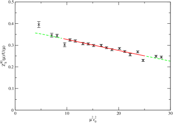
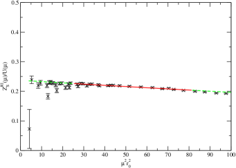
Figure 1: $Z_{S}^{\mathrm{RI-MOM}}(\mu)/U(\mu)$ on our coarsest and finest ($\beta\!=\!5.66,6.0$) lattice using the 1 HYP overlap operator with $\rho\!=\!1$. The solid line indicates a linear fit with range $3\!\leq\!\mu r_{0}\!\leq\!5$ and $5\!\leq\!\mu r_{0}\!\leq\!9$, respectively.

To compute the scalar and pseudoscalar renormalization constant we follow the non-perturbative RI-MOM procedure as defined in [19] and first applied to overlap fermions in [20, 21]. We compute both $Z_{S}(\mu)$ and $Z_{P}(\mu)$; in the latter case a $1/m$ term is used to extrapolate the result to the chiral limit. It turns out that the values obtained are in good agreement even on our coarsest lattice. We fit the scalar renormalization constant to the form

$$Z_{S}^{\mathrm{RI-MOM}}(\mu)=U(\mu)Z_{S}^{\mathrm{RGI}}+\mathrm{const}\,(a\mu)^{2}$$ (6)

where $U(\mu)$ is the 4-loop running in the RI-MOM scheme as given in [22] and the second term is introduced to account for discretization effects. In other words the scalar renormalization constant after dividing out the 4-loop perturbative running should be flat, up to discretization effects, and Fig. 1 shows that the latter are indeed non-negligible. The wiggles in the data signal rotational symmetry breaking on the lattice. We checked that within errors the slope disappears in proportion to $(a/r_{0})^{2}$. The phenomenological analysis below is based on $Z_{S}^{\mathrm{RI-MOM}}(2\,\mathrm{GeV})$, where $\mu\!=\!2\,\mathrm{GeV}$ is realized through $\mu r_{0}\!=\!5.06773$. The systematic error is estimated by varying the fit range, by including additional $1/p^{2}$ terms into the fit, and by comparing to the $Z_{P}^{\mathrm{RI-MOM}}(2\,\mathrm{GeV})$ data. A summary of our results, after conversion to $(\overline{\mathrm{MS}},2\,\mathrm{GeV})$ conventions, is presented in Tab. 3. Choosing a fixed $\rho\!>\!1$ would delay the breakdown of the unfiltered version – see [6] for details. Note that the $Z_{S}$ factors of all UV-filtered operators are much closer to $1$, even when compared to the unfiltered overlap operator with tuned $\rho$ [20, 23, 24]. This suggests that one should be able to compute renormalization constants perturbatively, as was done in [10] in a slightly different setup.

	$\beta=5.66$	$\beta=5.76$	$\beta=5.84$	$\beta=6.0$
none	ill-def.	ill-def.	6.14(15)(38)	2.54(6)(12)
1 APE	3.05(7)(34)	1.79(4)(6)	1.60(3)(8)	1.26(3)(8)
3 APE	2.05(7)(43)	1.35(4)(8)	1.25(2)(8)	1.04(2)(7)
1 HYP	1.71(4)(24)	1.24(3)(6)	1.23(2)(6)	1.03(2)(7)
3 HYP	1.57(6)(25)	1.16(3)(5)	1.10(2)(7)	0.98(2)(6)

Table 3: Renormalization constant $Z_{S}^{\overline{\mathrm{MS}}}(2\,\mathrm{GeV})$ for Wilson glue and $\rho\!=\!1$. The main effect of filtering is to bring it much closer to its tree-level value 1.

The second ingredient is the axial-vector renormalization constant $Z_{A}$. Here we use the values given in [6] (coming from a PCAC renormalization condition), complemented by a $\beta\!=\!5.76$ column included in [25]. It turns out that the values in this column are in fair agreement with the prediction by the Padé curve given in [6], which is another indication that for the filtered overlap operator lattice perturbation theory might work rather well.

3 Physical results

To extract meson masses and decay constants we compute the correlators

$$C_{\Gamma_{1},\Gamma_{2}}(t)=\sum_{\mathbf{x}}\langle\bar{\psi}_{1}(0)\Gamma_{1}\hat{\psi}_{2}(0)\bar{\psi}_{2}(\mathbf{x},t)\Gamma_{2}\hat{\psi}_{1}(\mathbf{x},t)\rangle$$ (7)

where

$$\hat{\psi}={1+{\gamma_{5}}\hat{{\gamma_{5}}}\over 2}\psi$$ (8)

denotes the “chirally rotated” quark field [5]. Specifically, we consider

$$\langle SS\rangle(t)=C_{1,1}(t)\;,\quad\langle PP\rangle(t)=C_{{\gamma_{5}},{\gamma_{5}}}(t)\;,\quad\langle A_{0}A_{0}\rangle(t)=C_{{\gamma_{5}}\gamma_{0},{\gamma_{5}}\gamma_{0}}(t)$$ (9)

and we extract the mass and decay constant of the pseudoscalar meson from fits to the $\langle A_{0}A_{0}\rangle$ and $\langle PP\rangle\!-\!\langle SS\rangle$ [26] channels. We do not consider $\langle PP\rangle$, since it is known to be contaminated by zero mode contributions [21, 27].

Generically, we see plateaus in the effective mass from about $N_{T}/4$ on, with the exception of the unfiltered operator, where the plateau sets in later and is less pronounced. Our central values stem from a fit to the $\langle A_{0}A_{0}\rangle$ correlator in the range $5N_{T}/16\!\leq\!t\!\leq\!11N_{T}/16$. The theoretical error is dominated by the comparison to $\langle PP\rangle\!-\!\langle SS\rangle$. Including only variations of the fit range (and below the error on $Z_{S}$), it would be much smaller.

In Fig. 2 the pseudoscalar meson mass squared is plotted versus the bare quark mass. Using regularly spaced quark masses, each $m_{1}\!+\!m_{2}$ combination is realized in several ways and the pertinent $M_{P}$ are in excellent agreement. In other words, isospin breaking effects are completely negligible. Therefore we fit the quark mass dependence of the pseudoscalar meson mass with the resummed quenched XPT expression [28]

$$M_{P}^{2}=A\,(m_{1}\!+\!m_{2})^{1/(1+\delta)}+B\,(m_{1}\!+\!m_{2})^{2}$$ (10)

which is strictly true only for degenerate masses. Our $\delta$ fluctuates wildly and is thus trivially consistent with 0.2 [28].

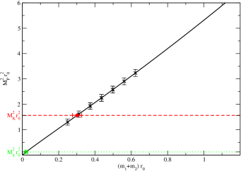
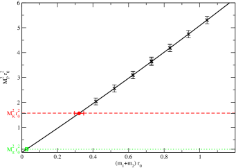
Figure 2: $M_{P}r_{0}$ versus the bare quark mass $(m_{1}\!+\!m_{2})r_{0}$ on our coarsest and finest ($\beta\!=\!5.66,6.0)$ lattice for the 1 HYP operator. The masses come from a fit to the $\langle A_{0}A_{0}\rangle$ correlator in the range $5N_{T}/16\!\leq\!t\!\leq\!11N_{T}/16$. The solid curve represents a fit to the functional form (10) and the horizontal lines indicate the physical $M_{\pi}r_{0}$ and $M_{K}r_{0}$ values. The latter are used to read off the fitted $2m_{ud}r_{0}$ and $(m_{s}\!+\!m_{ud})r_{0}$, respectively.

The next step requires some experimental input. Since we do not see any isospin breaking effects and electromagnetic corrections are of the order of 1%, while our statistical errors turn out to be roughly 10%, we decided to use the charged meson masses as input. Sticking to the identification $r_{0}\!=\!0.5\,\mathrm{fm}$ we use $M_{K}r_{0}\!=\!493.7\,\mathrm{MeV}\!\cdot 0.5\,\mathrm{fm}\!=\!1.251$ and $M_{\pi}r_{0}\!=\!139.6\,\mathrm{MeV}\!\cdot 0.5\,\mathrm{fm}\!=\!0.3537$ as input. This gives the bare $(m_{1}\!+\!m_{2})r_{0}$ values indicated by a horizontal error bar in Fig. 2. Multiplying the bare masses with the $Z_{m}\!=\!Z_{S}^{-1}$ obtained earlier, we extract the renormalized quark masses. Our results for $m_{s}\!+\!m_{ud}$ and $2m_{ud}$ are reported in Tabs. 5 and 5, respectively.

	$\beta=5.66$	$\beta=5.76$	$\beta=5.84$	$\beta=6.0$
none	ill-def.	ill-def.	0.219(34)(181)	0.378(36)(28)
1 APE	0.244(34)(45)	0.366(40)(50)	0.260(33)(19)	0.329(27)(31)
3 APE	0.260(21)(47)	0.311(32)(43)	0.223(32)(20)	0.312(26)(26)
1 HYP	0.301(25)(39)	0.336(35)(67)	0.240(28)(23)	0.321(26)(28)
3 HYP	0.281(20)(40)	0.321(31)(24)	0.247(31)(21)	0.321(26)(22)

Table 4: $(m_{s}\!+\!m_{ud})r_{0}$ in $(\overline{\mathrm{MS}},2\,\mathrm{GeV})$ conventions. For the $\rho\!=\!1$ thin link action at $\beta\!=\!5.66,5.76$ no $Z_{m}\!=\!Z_{S}^{-1}$ is available (cf. Tab. 3).

	$\beta=5.66$	$\beta=5.76$	$\beta=5.84$	$\beta=6.0$
none	ill-def.	ill-def.	0.006(05)(08)	0.027(09)(03)
1 APE	0.006(07)(09)	0.017(12)(13)	0.007(08)(04)	0.027(07)(04)
3 APE	0.012(05)(17)	0.014(10)(18)	0.007(07)(01)	0.023(06)(03)
1 HYP	0.021(07)(05)	0.021(08)(09)	0.011(07)(02)	0.026(07)(04)
3 HYP	0.014(08)(05)	0.028(12)(09)	0.009(06)(05)	0.022(05)(03)

Table 5: $2m_{ud}r_{0}$ in $(\overline{\mathrm{MS}},2\,\mathrm{GeV})$ conventions. For the $\rho\!=\!1$ thin link action at $\beta\!=\!5.66,5.76$ no $Z_{m}\!=\!Z_{S}^{-1}$ is available (cf. Tab. 3).

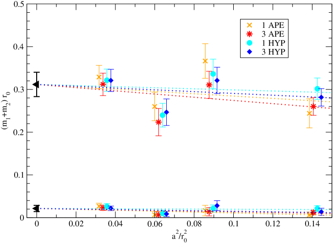
Figure 3: Renormalized $(\overline{\mathrm{MS}},2\,\mathrm{GeV})$ masses $(m_{s}\!+\!m_{ud})r_{0}$ and $2m_{ud}r_{0}$ versus $(a/r_{0})^{2}$. Errors are statistical, the 4 filterings are correlated (same configs.).

To finally push to the continuum we perform a combined fit (including all couplings and smearing levels) with a common continuum value and individual $O(a^{2})$ terms. We do this for the quantities $(m_{s}\!+\!m_{ud})r_{0}$, $2m_{ud}r_{0}$ (as shown in Fig. 3) as well as for $m_{s}r_{0}$ and $m_{s}/m_{ud}$. Our final result is

$$m_{s}(\overline{\mathrm{MS}},2\,\mathrm{GeV})r_{0}=0.301(25)(7)$$ (11)

in the continuum [$\chi^{2}\!/\mathrm{d.o.f.}\!=\!2.1$] which, upon using $r_{0}\!=\!0.5\,\mathrm{fm}$, leads to the result given in (2). For the ratio $m_{s}/m_{ud}$ we find the value quoted in (3) [$\chi^{2}\!/\mathrm{d.o.f.}\!=\!0.32$]. In either case the generic comment on statistical and systematic errors, as stated above, applies. Evidently, any result involving $m_{ud}$ benefits from our choice to use (10) at finite lattice spacing, since it restricts the curve in Fig. 2 to go through zero. The absence of curvature in our data is the reason why this ratio is in rather good agreement with the XPT result $m_{s}/m_{ud}\!=\!24.4(1.5)$ [29], in spite of the limitations mentioned and in spite of the latter value referring to a different theory (full QCD).

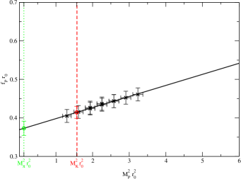
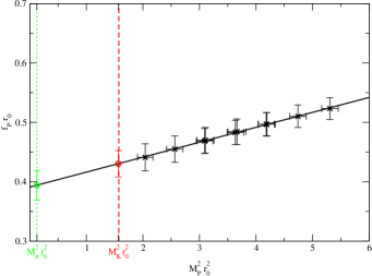
Figure 4: Pseudoscalar decay constant $f_{P}r_{0}$ versus $(M_{P}r_{0})^{2}$ on our coarsest and finest $(\beta=5.66,6.0)$ lattice for the 1 HYP overlap operator. $M_{P}$ and $f_{P}$ are obtained from a fit to the $\langle A_{0}A_{0}\rangle$ correlator in the region $T=\{5N_{T}/16,\ldots,11N_{T}/16\}$. The solid curve is a linear fit, the dotted vertical lines indicate the physical $M_{\pi}r_{0}$ and $M_{K}r_{0}$, respectively.

The pseudoscalar decay constant $f_{P}$ is extracted from the $\langle A_{0}A_{0}\rangle$ correlator. Generically, we see plateaus for the effective decay constant from about $N_{T}/4$ on, again with the exception of the unfiltered operator where they are less pronounced. We use the $Z_{A}$ values discussed earlier. Our central values stem from the interval $5N_{T}/16\!\leq\!t\!\leq\!11N_{T}/16$ and the error estimate comes from comparing to the $\langle PP\rangle\!-\!\langle SS\rangle$ channel, from varying the fit range and from the error on $Z_{A}$.

	$\beta=5.66$	$\beta=5.76$	$\beta=5.84$	$\beta=6.0$
none	ill-def.	ill-def.	0.575(39)(163)	0.422(19)(10)
1 APE	0.412(23)(69)	0.391(21)(10)	0.463(31)(35)	0.430(22)(26)
3 APE	0.426(18)(54)	0.398(20)(06)	0.449(33)(33)	0.433(22)(31)
1 HYP	0.414(15)(40)	0.398(21)(03)	0.446(32)(22)	0.430(22)(27)
3 HYP	0.400(15)(49)	0.378(16)(08)	0.419(28)(26)	0.430(22)(35)

Table 6: $f_{K}r_{0}$ on all lattices used in the continuum extrapolation and the unfiltered. With the $\rho\!=\!1$ thin link action at $\beta\!=\!5.66,5.76$ there is no signal.

	$\beta=5.66$	$\beta=5.76$	$\beta=5.84$	$\beta=6.0$
none	ill-def.	ill-def.	0.541(48)(211)	0.387(23)(19)
1 APE	0.367(37)(161)	0.356(24)(22)	0.438(45)(81)	0.393(25)(36)
3 APE	0.398(36)(133)	0.358(24)(28)	0.415(47)(66)	0.397(26)(42)
1 HYP	0.373(18)(69)	0.365(24)(14)	0.412(42)(33)	0.394(25)(36)
3 HYP	0.386(26)(118)	0.334(18)(07)	0.386(39)(55)	0.396(25)(45)

Table 7: $f_{\pi}r_{0}$ on all lattices used in the continuum extrapolation and the unfiltered. With the $\rho\!=\!1$ thin link action at $\beta\!=\!5.66,5.76$ there is no signal.

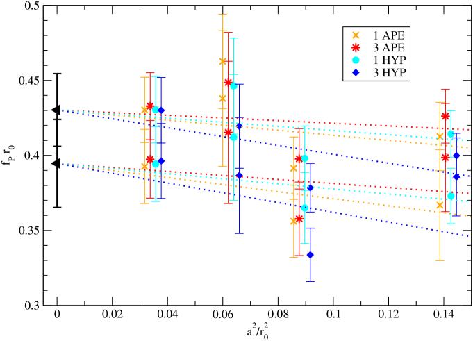
Figure 5: Pseudoscalar decay constants $f_{\pi}r_{0}$ and $f_{K}r_{0}$ versus $(a/r_{0})^{2}$. Errors are statistical, the 4 filterings are correlated (same configs.).

In Fig. 4 $f_{P}$ is plotted versus the meson mass squared. We see a strictly linear behavior at all couplings, with the lattice spacing having only mild effects on intercept and slope. Since (quenched) XPT predicts a linear dependence on $M_{P}^{2}$ at lowest order and (quenched) chiral logs enter at 1-loop level only, we decided to stick to the leading order and do a linear fit. The intercept with $(M_{K}r_{0})^{2}\!=\!1.251^{2}$ and $(M_{\pi}r_{0})^{2}\!=\!0.3537^{2}$ defines the $f_{K}r_{0}$ and $f_{\pi}r_{0}$ at finite lattice spacing reported in Tabs. 7 and 7, respectively.

To extrapolate to the continuum, the same recipe is used as before. A combined fit to all filtering levels with a common continuum limit and individual $O(a^{2})$ terms is shown in Fig. 5 for $f_{K}$ and $f_{\pi}$. We obtain

$$f_{K}r_{0}=0.430(24)(5)$$ (12)

in the continuum [$\chi^{2}\!/\mathrm{d.o.f.}\!=\!0.96$] which, via $r_{0}\!=\!0.5\,\mathrm{fm}$, yields (2). Applying the same strategy to $f_{K}/f_{\pi}$ we find the value quoted in (3) [$\chi^{2}\!/\mathrm{d.o.f.}\!=\!0.52$]. Given the large errors it is not so surprising that both $f_{K}$ and $f_{K}/f_{\pi}$ are in reasonable agreement with the experimental $f^{\mathrm{exp}}_{K}=159.8(1.5)\,\mathrm{MeV}$ and $f_{K}^{\mathrm{exp}}/f_{\pi}^{\mathrm{exp}}=1.223(12)$, respectively [30]. Especially in the latter case, higher precision would likely reveal a genuine quenching error [31].

4 Conclusion

We have presented an exploratory scaling study with UV-filtered overlap quarks, concentrating on the quenched continuum limit of the light quark masses and the $\pi$ and $K$ decay constants. The focus is not so much on the numerical values obtained; the point is that a nice scaling behavior has been observed down to lattices as coarse as $a^{-1}\!\simeq\!1\,\mathrm{GeV}$. As anticipated in [6] the details of the filtering recipe play a minor role and therefore we conjecture that with analytic gauge link smearing techniques [32] these properties will carry over to dynamical overlap calculations (cf. [33, 34, 35]).

For the time being let us mention that the simulations were done on a few of todays standard PCs (3 GHz Pentium 4), using an equivalent of $\sim\!120$ days on one such PC for the 1 APE operator (including all couplings) and of $\sim\!60$ days for any of the other filtered operators. With a complete scaling study based on overlap valence quarks requiring less than 1 PC year one is tempted to ask whether for some phenomenological questions the overlap might actually represent the cheapest approach to obtain a continuum result.

Acknowledgments: This work is based on an earlier collaboration with Urs Wenger that lead to [6]. S.D. was supported by the Swiss NSF.

References

- [1]
- [2] H. Neuberger, Phys. Lett. B 417, 141 (1998) [hep-lat/9707022].
- [3] P.H. Ginsparg and K.G. Wilson, Phys. Rev. D 25, 2649 (1982).
- [4] P. Hasenfratz, V. Laliena and F. Niedermayer, Phys. Lett. B 427, 125 (1998) [hep-lat/9801021].
- [5] M. Lüscher, Phys. Lett. B 428, 342 (1998) [hep-lat/9802011].
- [6] S. Dürr, C. Hoelbling and U. Wenger, hep-lat/0506027.
- [7] W. Bietenholz, hep-lat/0007017.
- [8] T.G. Kovács, hep-lat/0111021.
- [9] T.G. Kovács, Phys. Rev. D 67, 094501 (2003) [hep-lat/0209125].
- [10] T. DeGrand, Phys. Rev. D 67, 014507 (2003) [hep-lat/0210028].
- [11] S.J. Dong, F.X. Lee, K.F. Liu and J.B. Zhang, Phys. Rev. Lett. 85, 5051 (2000) [hep-lat/0006004].
- [12] J. Gasser and H. Leutwyler, Annals Phys. 158, 142 (1984).
- [13] M. Albanese et al. [APE Collab.], Phys. Lett. B 192, 163 (1987).
- [14] A. Hasenfratz and F. Knechtli, Phys. Rev. D 64, 034504 (2001) [hep-lat/0103029].
- [15] A. Hasenfratz, R. Hoffmann and F. Knechtli, Nucl. Phys. Proc. Suppl. 106, 418 (2002) [hep-lat/0110168].
- [16] S. Dürr, C. Hoelbling and U. Wenger, Phys. Rev. D 70, 094502 (2004) [hep-lat/0406027].
- [17] R. Sommer, Nucl. Phys. B 411, 839 (1994) [hep-lat/9310022].
- [18] M. Guagnelli, R. Sommer and H. Wittig [ALPHA Collab.], Nucl. Phys. B 535, 389 (1998) [hep-lat/9806005].
- [19] G. Martinelli, C. Pittori, C.T. Sachrajda, M. Testa and A. Vladikas, Nucl. Phys. B 445, 81 (1995) [hep-lat/9411010].
- [20] L. Giusti, C. Hoelbling and C. Rebbi, Nucl. Phys. Proc. Suppl. 106, 739 (2002) [hep-lat/0110184].
- [21] L. Giusti, C. Hoelbling and C. Rebbi, Phys. Rev. D 64, 114508 (2001), Erratum-ibid. D 65, 079903 (2002) [hep-lat/0108007].
- [22] K.G. Chetyrkin and A. Retey, Nucl. Phys. B 583, 3 (2000) [hep-ph/9910332].
- [23] P. Hernandez, K. Jansen, L. Lellouch and H. Wittig, JHEP 0107, 018 (2001) [hep-lat/0106011].
- [24] J. Wennekers and H. Wittig, hep-lat/0507026.
- [25] S. Dürr, C. Hoelbling and U. Wenger, hep-lat/0509111.
- [26] T. Blum et al., Phys. Rev. D 69 (2004) 074502 [hep-lat/0007038].
- [27] C. Gattringer et al. [BGR Collab.], Nucl. Phys. B 677, 3 (2004) [hep-lat/0307013].
- [28] S.R. Sharpe, Phys. Rev. D 46, 3146 (1992) [hep-lat/9205020].
- [29] J. Gasser and H. Leutwyler, Phys. Rept. 87, 77 (1982).
- [30] K. Hagiwara et al. [PDG Collab.], Phys. Rev. D 66, 010001 (2002).
- [31] S. Aoki et al. [CP-PACS Collaboration], Phys. Rev. D 67, 034503 (2003) [hep-lat/0206009].
- [32] C. Morningstar and M.J. Peardon, Phys. Rev. D 69, 054501 (2004) [hep-lat/0311018].
- [33] T. DeGrand and S. Schaefer, Phys. Rev. D 71, 034507 (2005) [hep-lat/0412005].
- [34] T. DeGrand and S. Schaefer, hep-lat/0506021.
- [35] Y. Aoki, Z. Fodor, S.D. Katz and K.K. Szabo, proceedings of Lattice 2005 and paper in preparation.