Balance of baryon number
in the quark coalescence model

Abstract

The charge and baryon balance functions are studied in the coalescence hadronization mechanism of quark-gluon plasma. Assuming that in the plasma phase the $q\bar{q}$ pairs form uncorrelated clusters whose decay is also uncorrelated, one can understand the observed small width of the charge balance function in the Gaussian approximation. The coalescence model predicts even smaller width of the baryon-antibaryon balance function: $\sigma_{B\bar{B}}/\sigma_{+-}=\sqrt{2/3}$.

1. Introduction

It was recently argued [1] that the constituent quark coalescence model [2] can explain the small pseudo-rapidity width of the charge balance function [3, 4] observed in central collisions of heavy ions at RHIC [5], as compared to that measured in pp collisions [3]. The charge (or baryon number) balance function measures the relative distance between produced positive and negative charges. Encouraged by the success of this simple argument, in the present paper we apply the same idea to the balance function measuring the baryon-antibaryon compensation.

Our aim is to discuss correlations between produced hadrons, and thus the quark coalescence model must be generalized to consider possible preexistent correlations inside the system. In a state rich in quark-antiquark pairs arising from initial (charge and flavor neutral) gluon fragmentation we can supplement the standard formulation of the model by the hypothesis that -before hadronization- the QGP forms charge- and flavor-neutral $q\bar{q}$-clusters, which seems natural in a gluon-dominated plasma. In the final, pre-hadronization stage the clusters dissociate, quarks and antiquarks coalesce into observed hadrons while gluons required to balance color charge form additional neutral quark clusters (and again gluons) and the process is repeated till hadronization is completed.

For this reason we can assume for the purpose of evaluating the balance correlation that at the last stage before hadronization the plasma consists of isotropic $q\bar{q}$ clusters which are charge-, flavor- and (though natural, here important) baryon number- neutral. In the coalescence model a charged meson is formed from two such $q\bar{q}$ clusters. The charged bosons final state balance function is thus reduced by a factor $1/\sqrt{2}$ with respect to the width of source distributions, since as is well known, the width of the distribution of the average of any two independent variables ($q$, $\bar{q}$ in different $q\bar{q}$) is reduced by the factor $1/\sqrt{2}$ with respect to the width of their own distributions. This was the argument in Ref. [1].

Here we observe that since baryons are formed from three constituent quarks, we expect in this case a reduction by a factor $1/\sqrt{3}$, and thus an even further reduction (by the factor $\sqrt{2/3}$ beyond charge balance narrowing) of the width of the baryon balance function. A particularly interesting case is the balance function of neutral strange baryons ($\Lambda(sud)$) since the coalescence formation requires here under any possible microscopic mechanism the participation of three independent ($s\bar{s},\,u\bar{u},\,d\bar{d}$) neutral quark clusters.

The confirmation of this prediction by the future data could be considered as an important indication that the coalescence model is the dominant mechanism in the hadronization of the quark-gluon plasma. The coalescence model is the key ingredient required to describe the relative yields of hadrons within the statistical hadronization approach [6]: the probability of production of a hadron is by assumption a product of probabilities of finding the constituent quarks of the hadron considered.

With this formulation all consequences of the coalescence model concerning single particle distributions are of course unchanged. In particular, the spectacular successes of the model in description of single particle spectra [2, 7] and flow parameters [8] in the central collisions of heavy ions remain valid. Thus our extension is a natural attempt to make the coalescence model more complete.

To proceed, we need to define some properties of the neutral clusters. To keep the discussion as simple as possible, we shall assume that (i) a cluster decays isotropically in its rest frame, and (ii) momenta of the decay products are uncorrelated. These two properties are sufficient to derive most of our conclusions. To keep the problem as simple as possible, we shall also assume that the clusters themselves are uncorrelated, as would be expected if these arise from gluons.

Using this scenario, we give predictions for the (pseudo)rapidity width of the charge and baryon balance functions, including corrections due to the finite acceptance region. In the next section 2. Balance functions we introduce the notation. The analysis of the charge balance function given in [1] is shortly summarized in section 3. Estimate of the baryon balance function is given in section 4. Our conclusions are listed in the last section.

2. Balance functions

In this paper we shall only discuss the neutral systems, u.e. the systems with vanishing total charge and baryon number. In this case the balance function of the “charges” denoted by $+$ and $-$ is expressed in terms of the single- $N$ and double- $D$ particle functions [4, 9] as follows:

$$B(\Delta_{2}|\Delta_{1}) = \frac{D(+,\Delta_{2}|-,\Delta_{1})-D(+,\Delta_{2}|+,\Delta_{1})}{N_{+}(\Delta_{1})}+$$ (1)

$$+ \frac{D(-,\Delta_{2}|+,\Delta_{1})-D(-,\Delta_{2}|-,\Delta_{1})}{N_{-}(\Delta_{1})}.\l{9}$$

Here

$$D(i,\Delta_{2}|j,\Delta_{1})=\int_{\Delta_{2}}dy_{2}\int_{\Delta_{1}}dy_{1}\frac{d^{2}n_{ij}}{dy_{1}dy_{2}}\l{7}$$ (2)

$$N_{i}(\Delta)=\int_{\Delta}\frac{dN_{i}}{dy}dy\l{7a}$$ (3)

where $dn_{i}/dy$ and $dn^{2}_{ij}/dy_{1}dy_{2}$ are the corresponding particle densities.

The measurement of the electric charge balance function performed by the STAR collaboration requires both particles to be in a finite rapidity acceptance interval $-\Delta\leq y_{1},y_{2}\leq\Delta$ while the difference $\delta$ of (pseudo)rapidities is kept fixed. This suggests a change of variables:

$$y_{1}-y_{2}\equiv\delta;\qquad{y_{1}+y_{2}\over 2}\equiv z.\l{ix}$$ (4)

With this notation, the integration in Eq. (LABEL:7) must be restricted to $\delta$ being fixed, while $z$ must be kept inside the interval $-\bar{\Delta}\leq z\leq\bar{\Delta}$ where

$$\bar{\Delta}=\Delta-{|\delta|\over 2}.\l{ixa}$$ (5)

We shall use this prescription also for the baryon number which is of interest in this paper.

Thus the balance function we discuss is defined as

$$B_{s}(\delta;\Delta) = \frac{\int_{-\bar{\Delta}}^{-\bar{\Delta}}dz\left[d^{2}n_{+-}/dzd\delta-d^{2}n_{++}/dzd\delta\right]}{\int_{-\Delta}^{+\Delta}dy_{+}dn_{+}/dy_{+}}+$$ (6)

$$+ \frac{\int_{-\bar{\Delta}}^{-\bar{\Delta}}dz\left[d^{2}n_{-+}/dzd\delta-d^{2}n_{--}/dzd\delta\right]}{\int_{-\Delta}^{+\Delta}dy_{-}dn_{-}/dy_{-}}\l{i5}$$

where $\pm$ refers here to the baryon number.

3. Balance function in the coalescence model

We first consider the production of charged pions [1]. In formation of such a pair, the dominant process is that involving one $U$-cluster and one $D$-cluster:

$$(u\bar{u})+(d\bar{d})\;\rightarrow\;(u\bar{d})+(\bar{u}d).\l{m1}$$ (7)

The corresponding two particle momentum distribution is:

$$\rho(p_{+},p_{-}) = \int dP_{1}dP_{2}\rho_{c}(P_{1})\rho_{c}(P_{2})\int dp_{u_{1}}d\bar{p}_{u_{1}}dp_{d_{2}}d\bar{p}_{d_{2}}$$ (8)

$$f(P_{1},p_{u_{1}})f(P_{1},\bar{p}_{u_{1}})f(P_{2},p_{d_{2}})f(P_{2},\bar{p}_{d_{2}})$$

$$\delta[p_{+}-(p_{u_{1}}+\bar{p}_{d_{2}})/2]\delta[p_{-}-(\bar{p}_{u_{1}}+p_{d_{2}})/2]$$

$$G_{m}(p_{u_{1}}-\bar{p}_{d_{2}})G_{m}(p_{d_{1}}-\bar{p}_{u_{2}})\l{m2}$$

where $\rho_{c}(P)$ is the distribution of clusters, $f(P,p)$ the cluster dissociation probability, that is the probability of finding a quark of momentum $p$ in the cluster of momentum $P$, and $G(p-\bar{p})$ is the probability of coalescence, i.e. that a quark-antiquark pair forms a hadron. The momenta of quarks are denoted by $p$, those of antiquarks by $\bar{p}$.

Since one pair of clusters cannot produce two mesons of the same charge, only $\rho(p_{+},p_{-})$ given by (LABEL:m2) contributes to the balance function. In the following we shall only consider rapidity and pseudo-rapidity distributions. To simplify the technicalities we take all functions in (LABEL:m2) in the Gaussian form:

$$\rho_{c}(Y)=\frac{N}{A\sqrt{\pi}}e^{-Y^{2}/A^{2}}\;;\;\;f(Y,y)=\frac{1}{c\sqrt{\pi}}e^{-(Y-y)^{2}/c^{2}}\;;\;\;\l{m3}$$ (9)

where $N$ is the total number of clusters. It turns out that the balance function does not depend on the shape of $G(u)$.

Introducing (LABEL:m3) into (LABEL:m2) allows to perform all integrations. The result, substituted in (LABEL:i5), gives

$$B_{m}(\delta;\Delta)=\frac{1}{c\sqrt{\pi}}e^{-\delta^{2}/c^{2}}\frac{\rm erf[2\bar{\Delta}/\sqrt{2A^{2}+c^{2}}]}{\rm erf[2\Delta/\sqrt{2A^{2}+2c^{2}}]}\l{m4}$$ (10)

One sees that in the limit of large acceptance ($\Delta\rightarrow\infty$) the width of the balance function is determined by the same parameter $c$ which describes the cluster dissociation width. The effect of finite acceptance, $\Delta$, is seen as the ratio of the two error functions. Note that in the Gaussian distribution model the balance function is entirely independent of the coalescence probability distribution $G(u)$.

4. Baryon balance function

The dominant process in the production of baryon-antibaryon pairs involves three clusters:

$$(q\bar{q})+(q\bar{q})+(q\bar{q})\;\rightarrow\;(qqq)+(\bar{q}\bar{q}\bar{q})\l{b1}$$ (11)

Consequently, the distribution of the $B\bar{B}$ pair is:

$$\rho(p,\bar{p}) = \int dP_{1}dP_{2}dP_{3}\rho_{c}(P_{1})\rho_{c}(P_{2})\rho_{c}(P_{3})\int dp_{1}dp_{2}dp_{3}d\bar{p}_{1}d\bar{p}_{2}d\bar{p}_{3}$$ (12)

$$f(P_{1},p_{1})f(P_{2},p_{2})f(P_{3},p_{3})f(P_{1},\bar{p}_{1})f(P_{2},\bar{p}_{2})f(P_{3},\bar{p}_{3})$$

$$\delta[p-(p_{1}+p_{2}+p_{3})/3]\delta[\bar{p}-(\bar{p}_{1}+\bar{p}_{2}+\bar{p}_{3})/3]$$

$$G_{B}(p_{1}-p_{2},p_{2}-p_{3},p_{3}-p_{1})G_{B}(\bar{p}_{1}-\bar{p}_{2},\bar{p}_{2}-\bar{p}_{3},\bar{p}_{3}-\bar{p}_{1}).\qquad\l{b2}$$

Introducing Eq. (LABEL:m3) into Eq. (LABEL:b2), performing the integrations and putting the result into Eq. (LABEL:i5), one obtains:

$$B_{B}(\delta;\Delta)=\frac{\sqrt{3}}{c\sqrt{2\pi}}\,e^{-3\delta^{2}/(2c^{2})}\,\frac{\rm erf[\sqrt{6}\,\bar{\Delta}/\sqrt{2A^{2}+c^{2}}]}{\rm erf[\sqrt{3}\Delta/\sqrt{A^{2}+c^{2}}]}\,.\l{b3}$$ (13)

One sees that in the limit of large acceptance the width of baryon balance function is again determined by the parameter $c$ but it is by the factor $\sqrt{2/3}$ smaller than that for obtained for the charged pion balance functions given by Eq. (LABEL:m4). The corrections due to finite acceptance are also given by ratio of two error functions but their arguments are multiplied by $\sqrt{3/2}$, as compared to those in Eq. (LABEL:m4). Therefore they are slightly less important than in the pion case.

It is natural to expect that the $(q\bar{q})$ cluster dissociation probability is isotropic. As discussed in [1], this puts a strong constraint on the parameter $c$ responsible for the cluster decay distribution. Indeed, the isotropic decay implies that the decay distribution in pseudo-rapidity is

$$\rho(\eta)\approx\frac{1}{2(\cosh\eta)^{2}}\,,\l{i10}$$ (14)

corresponding to the (pseudo)rapidity distribution of statistically produced (massless) particles. The width of this distribution is $\langle|\eta|\rangle\equiv\int d\eta|\eta|\rho(\eta)=\log 2\approx 0.69$. In order to approximate the distribution (LABEL:i10) by a Gaussian of the same width we must use:

$$c=\sqrt{\pi}\log 2\approx 1.23\,.\l{n1}$$ (15)

Although Eq. (LABEL:n1) refers to pseudo-rapidity distribution, we shall take this value of $c$ to describe as well the rapidity distribution in cluster decay. As shown in [1], this value is compatible with the STAR data [5], provided that the finite acceptance corrections are included ($A=3.5$ was assumed). These corrections are important: they reduce the width from $0.69$ to $0.55$, compatible with data.

The comparison of the results for charge and baryon balance functions is shown in Fig. 1 where the expected widths, calculated from Eq. (LABEL:m4) and Eq. (LABEL:b3) with $c$ given by Eq. (LABEL:n1) and $\Delta=1.3$, are plotted as function of the cluster distribution width $A$, to show (in)sensitivity with regard to the cluster distribution. Also in Fig. 1 the ratio of the charge (m: meson) and baryon balance function widths is shown.

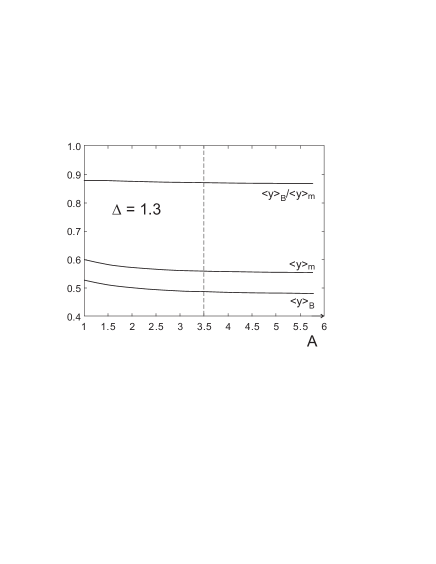
Figure 1: Widths of balance functions versus the width $A$ of the pre-hadronization cluster rapidity distribution.

As discussed in Ref. [1], $\langle|y|\rangle$ for pions agrees reasonably well with the STAR data in a rather broad range of $A$. One also sees that the ratio of baryon and pion widths is predicted to be $.87$ and is insensitive to $A$. This value is larger than $\sqrt{(}2/3)\approx.82$, expected for large rapidity acceptance.

In Fig. 2 the same quantities are plotted versus $\Delta$, the size of the acceptance region for $A=3.5$. One sees that the widths change rather rapidly when $\Delta$ varies from 1 up to 3. Starting from $\Delta=4$ the effect of acceptance practically disappears.

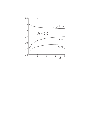
Figure 2: Widths of balance functions versus the acceptance $\Delta$. Vertical dashed line indicates the STAR acceptance.

5. Comments and conclusions

Several comments are in order.

(i) We have ignored the transverse motion of the clusters (the distribution (LABEL:i10) is only valid for clusters with vanishing transverse momentum). The effect of transverse motion is expected to reduce the decay width in rapidity [10]. This effect was discussed in Ref. [1] and shown to be small for transverse velocities up to 0.4 . It may be interesting, however, to investigate -both theoretically and experimentally- the balance functions at larger transverse momenta. Such studies may provide additional information about the properties of the transverse flow.

(ii) We have also ignored the difference between rapidity and pseudo-rapidity. Therefore, our predictions of the balance function width in rapidity could be somewhat overestimated. The width ratio between baryons and pions is, however, much less sensitive to this effect and thus remains a much more solid prediction.

(iii) The correlations in cluster decay were neglected. As shown in [1], introducing correlations may change somewhat the width of the balance functions. This may be an interesting point for future research.

(iv) As we were using Gaussian approximation, we cannot discuss seriously the shape of the balance function. Although the present data are consistent with Gaussian shapes, it would be interesting to investigate the problem more thoroughly when better data become available.

(v) We have only considered the dominant processes leading to meson and baryon formation. The corrections from sub-dominant ones give, generally, contributions to balance functions which are much broader than those described in the present paper.

(vi) The effect of resonance decay was entirely neglected. This serious problem seems, however, beyond reach of our approach. In this context, it should be emphasized that the argument presented in this paper applies to any kind of baryon-antibaryon pairs. Thus we feel that measurements of (multi)strange baryons may be particularly interesting, because -due to their large mass- they are less sensitive to corrections related to resonance decays and transverse motion.

In conclusion, we have calculated the width of the charge and baryon number balance functions in the coalescence model generalized to include possibility of correlations between constituent quarks and antiquarks in the form of charge- and flavor- neutral, isotropically dissociating clusters. The existing data on charge balance functions are explained. The width of the baryon balance function at large acceptance is predicted to be smaller by nearly a factor $\sqrt{2/3}$. Finite acceptance corrections were estimated. We believe that future measurements of the baryon balance functions may provide an interesting test of the quark coalescence hadronization model.

References

- [1] A.Bialas, Phys. Lett. B579 (2004) 31.
- [2] T.S.Biro, P.Levai and J.Zimanyi, Phys. Lett. B347 (1995) 6; J.Zimanyi, P.Levai and T.S.Biro Heavy Ion Phys. 17 (2003) 205 and references quoted there; J.Pisut, N.Pisutova, Acta Phys. Pol. B28 (1997) 2817; R.Lietava and J. Pisut, Eur. Phys. J. C5 (1998) 135. For a recent review, see W.Ochs, Acta Phys. Pol. B36 (2005) 761.
- [3] See, e.g., D.Drijard et al., Nucl.Phys. B155 (1979) 269; Nucl. Phys. B166 (1980) 233.
- [4] S.A.Bass, P.Danielewicz and S.Pratt, Phys. Rev. Lett. 85 (2000) 2689; S.Pratt,Nucl. Phys. A698 (2002) 531c; Nucl.Phys. A715 (2003) 389c.
- [5] STAR coll., J.Adams et al., Phys. Rev. Lett. 90 (2003) 172301.
- [6] J. Rafelski, Phys. Lett. B262, 333 (1991); G. Torrieri, W. Broniowski, W. Florkowski, J. Letessier and J. Rafelski, Comp. Phys. Com. 167, 229 (2005), and references therein.
- [7] See, e.g., A.Bialas, Phys. Lett. B442 (1998) 449; J.Zimanyi et al., Phys. Lett. B472 (2000) 243; J.Zimanyi, P.Levai and T.S.Biro, J.Phys. G28 (2002) 1561; J.Phys. G31 (2005) 551.
- [8] S.A.Voloshin, Nucl.Phys. A715 (2003) 379; D.Molnar and S.A.Voloshin, Phys. Rev. Lett. 91 (2003) 092301; S.A.Volishin, Acta Phys. Pol. B36 (2005) 551.
- [9] S.Jeon and S.Pratt, Phys. Rev. C65 (2002) 044902; T.Trainor, hep-ph/0301122; S.Jeon and V.Koch, hep-ph/0304012.
- [10] K.Zalewski, Acta Phys. Pol. B9 (1978) 87.