Distinguishing Between Hierarchical and Lop-sided SO(10) Models.

Abstract

A comparative study of two predictive SO(10) models , namely the BPW model (proposed by Babu, Pati and Wilczek) and the AB model (proposed by Albright and Barr) is done based on their predictions regarding CP and flavor violations. There is a significant difference in the structure of the fermion mass-matrices in the two models (which are hierarchical for the BPW case and lop-sided for the AB model) which gives rise to different CP and flavor violating effects. We include both SM and SUSY contributions to these processes. Assuming flavor universality of SUSY breaking parameters at a messenger scale $M^{*}\buildrel>\over{{}_{\sim}}M_{GUT}$, it has been shown that renormalization group based post-GUT physics gives rise to large CP and flavor violations. While these effects were calculated for the BPW model recently, this is the first time (to our knowledge) that post-GUT contributions have been included for the AB model. The values of $\Delta m_{K},\epsilon_{K},\Delta m_{B_{d}}$ and $S(B_{d}\to J/\psi K_{S})$ are found, in both models, to be close to SM predictions, in good agreement with data. Both models predict that $S(B_{d}\to\phi K_{S})$ should lie in the range +0.65–0.74, close to the SM prediction and that the EDM of the neutron $\approx(few\times 10^{-26})$e-cm, which should be observed in upcoming experiments. The lepton sector brings out marked differences between the two models. It is found that $Br(\mu\to e\gamma)$ in the AB model is generically much larger than that in the BPW model, being consistent with the experimental limit only with a rather heavy SUSY spectrum with $(m_{o},~{}m_{1/2})\sim(1000,~{}1000)$ GeV. The BPW model, on the other hand, is consistent with the SUSY spectrum being as light as $(m_{o},~{}m_{1/2})\sim(600,~{}300)$ GeV. Another distinction arises in the prediction for the EDM of the electron. In the AB model $d_{e}$ should lie in the range $10^{-27}-10^{-28}$e-cm, and should be observed by forthcoming experiments. The BPW model gives $d_{e}$ to be typically 100 times lower than that in the AB case. Thus the two models can be distinguished based on their predictions regarding CP and flavor violating processes, and can be tested in future experiments.

1 Introduction

Grand unified theories [1, 2, 3] have found much success in explaining (a) the quantum numbers of the members in a family, (b) quantization of electric charge and (c) the meeting of the gauge couplings at a scale $\sim 2\times 10^{16}$ GeV in the context of supersymmetry [4, 5]. In particular, it has been argued [6] that the features of (d) neutrino oscillations [7, 8], (e) the likely need for baryogenesis via leptogenesis [9, 10], and (f) the success of certain mass relations like $m_{b}\approx m_{\tau}$ and $m(\nu_{\tau})_{\rm Dirac}\approx m_{t}$ at the unification scale, suggest that the effective symmetry near the string/GUT scale in 4D should possess the symmetry SU(4)-color [2]. Thus, it should be either SO(10) [11] or minimally G(224) = $SU(2)_{L}\times SU(2)_{R}\times SU(4)^{c}$ [2]. (For a detailed review of the advantages and successes of G(224)/SO(10) symmetry, see e.g. [6].)

In recent years, several models based on supersymmetric SO(10) GUT have emerged [12]. Two promising candidates have been proposed which have much similarity in their Higgs structure and yet important differences in the pattern of fermion mass-matrices. One is by Albright and Barr (AB)[13] and the other by Babu, Pati and Wilczek (BPW) [14]. Both models use low-dimensional Higgs multiplets (like $45_{H},16_{H},\overline{16_{H}}$ and $10_{H}$) to break SO(10) and generate fermion masses (see remarks later) as opposed to large-dimensional ones (like $126,\overline{126},210$ and possibly 120). Both of these models work extremely well in making predictions regarding the masses of quarks and leptons, the CKM elements and neutrino masses and their mixings in good accord with observations. Nevertheless there is a significant difference between these two models in the structure of their fermion mass matrices. In the BPW-model, the elements of the fermion mass-matrices (constrained by a U(1)-flavor symmetry [15, 6, 16]) are consistently family-hierarchical with “33”$\gg$“23”$\sim$“32”$\gg$“22”$\gg$“12”$\sim$“21”$\gg$“11” etc. By contrast, in the AB-model, the fermion mass-matrices are lopsided with “23”$\sim$“33” in the down quark mass-matrix and “32”$\sim$“33” in the charged lepton matrix. (The exact structure of the fermion mass-matrices will be presented in Sec. 2.) This difference in the structure of the mass matrices leads to two characteristically different explanations for the largeness of the $\nu_{\mu}-\nu_{\tau}$ oscillation angle in the two models. For the BPW model, both charged lepton and neutrino sectors give moderately large contributions to this mixing which, as they show, naturally add to give a nearly maximal $\sin^{2}2\theta_{\nu_{\mu}-\nu_{\tau}}$, while simultaneously giving small $V_{cb}$ as desired. The largeness of $\theta_{\nu_{\mu}-\nu_{\tau}}$, together with the smallness of $V_{cb}$ (in the BPW model) turns out in fact to be a consequence of (a) the group theory of SO(10)/G(224) in the context of the minimal Higgs system, and (b) the hierarchical pattern of the mass-matrices. For the lopsided AB model, on the other hand, the large (maximal) $\nu_{\mu}-\nu_{\tau}$ oscillation angle comes almost entirely from the charged lepton sector which has a “32” element comparable to the “33”.

The original work of Babu, Pati and Wilczek, treated the entries in the mass matrices to be real for simplicity, thereby ignoring CP non-conservation. It was successfully extended to include CP violation by allowing for phases in the mass matrices by Babu, Pati and the author in Ref. [16].

The purpose of this paper is to do a comparative study between certain testable predictions of the AB model versus those of the BPW model allowing for the extension of the latter as in Ref. [16]. We find that while both models give similar predictions regarding fermion masses and mixings, they can be sharply distinguished by lepton flavor violation, especially by the rate of $\mu\to e\gamma$ and the edm of the electron.

We work in a scenario as in Refs. [16] and [17], in which flavor-universal soft SUSY breaking is transmitted to the sparticles at a messenger-scale M^∗, with M${}_{GUT}<$ M${}^{*}\leq$ M_string as in a mSUGRA model [18]. Following the general analysis in Ref. [19] it was pointed out in Refs. [16] and [17] that in a SUSY-GUT model with a high messenger scale as above, post-GUT physics involving RG running from M${}^{*}\to$ M_GUT leads to dominant flavor and CP violating effects. In the literature, however, post-GUT contribution has invariably been omitted, except for Refs. [16] and [17], where it has been included only for the BPW model. Lepton flavor violation in the AB model has been studied so far by many authors by including the contribution arising only through the RH neutrinos [20], without, however, the inclusion of post-GUT contributions. I therefore make a comparative study of the BPW and the AB models by including the contributions arising from both post-GUT physics, as well as those from the RH neutrinos through RG running below the GUT scale. For the sake of comparison and completeness, we will include the results obtained in Refs. [16] and [17] which deal with CP and flavor violation in the BPW model.

To calculate the branching ratio of lepton flavor violating processes we include contributions from three different sources: (i) the sfermion mass-insertions, $\hat{\delta}^{ij}_{LL,RR}$, arising from renormalization group (RG) running from M^∗ to M${}_{GUT}\sim 2\times 10^{16}$ GeV, (ii) the mass-insertions $(\delta^{ij}_{LL})^{RHN}$ arising from RG running from M_GUT to the right handed neutrino mass scales M${}_{R_{i}}$, and (iii) the chirality-flipping mass-insertions $\delta^{ij}_{LR,RL}$ arising from $A-$terms that are induced solely through RG running from M^∗ to M_GUT involving SO(10) or G(224) gauginos in the loop.

It was found in Ref. [17], that for the BPW-model, contributions to the rate of $\mu\to e\gamma$ from sources (i) and (iii) associated with post-GUT physics, were typically much larger than that from source (ii) associated with the RH neutrinos. For the AB-model, we find that the RH neutrino contribution is strongly enhanced compared to that in the BPW model; as a result all the three contributions to the amplitude of $\mu\to e\gamma$ are comparable. Including all three contributions, we find that for most of the SUSY parameter space, the branching ratio for $\mu\to e\gamma$ calculated in the AB-model is much larger than that in the BPW model and is in fact excluded by the experimental upper bound unless $(m_{o},\ m_{1/2})\buildrel>\over{{}_{\sim}}$ 1 TeV. Thus one main result of this paper is that, with all three sources of lepton flavor violation included, the process $\mu\to e\gamma$ can provide a clear distinction between the BPW and the AB models. We also examine CP violation as well as flavor violation in the quark sector, including that reflected by electric dipole moments, in the AB model, and compare it with the corresponding results for the BPW-model, obtained in [16].

In the following section the patterns of the fermion mass matrices for the BPW and the AB models are presented.

2 A brief description of the BPW and the AB models

The Babu-Pati-Wilczek (BPW) model

The Dirac mass matrices of the sectors $u,d,l$ and $\nu$ proposed in Ref. [14] in the context of SO(10) or G(224)-symmetry have the following structure:

$$\begin{array}[]{cc}M_{u}=\left[\begin{array}[]{ccc}0&\epsilon^{\prime}&0\\ -\epsilon^{\prime}&\zeta_{22}^{u}&\sigma+\epsilon\\ 0&\sigma-\epsilon&1\end{array}\right]{\cal M}_{u}^{0};&M_{d}=\left[\begin{array}[]{ccc}0&\eta^{\prime}+\epsilon^{\prime}&0\\ \eta^{\prime}-\epsilon^{\prime}&\zeta_{22}^{d}&\eta+\epsilon\\ 0&\eta-\epsilon&1\end{array}\right]{\cal M}_{d}^{0}\\ &\\ M_{\nu}^{D}=\left[\begin{array}[]{ccc}0&-3\epsilon^{\prime}&0\\ 3\epsilon^{\prime}&\zeta_{22}^{u}&\sigma-3\epsilon\\ 0&\sigma+3\epsilon&1\end{array}\right]{\cal M}_{u}^{0};&M_{l}=\left[\begin{array}[]{ccc}0&\eta^{\prime}-3\epsilon^{\prime}&0\\ \eta^{\prime}+3\epsilon^{\prime}&\zeta_{22}^{d}&\eta-3\epsilon\\ 0&\eta+3\epsilon&1\end{array}\right]{\cal M}_{d}^{0}\\ \end{array}$$ (16)

These matrices are defined in the gauge basis and are multiplied by $\bar{\Psi}_{L}$ on left and $\Psi_{R}$ on right. For instance, the row and column indices of $M_{u}$ are given by $(\bar{u}_{L},\bar{c}_{L},\bar{t}_{L})$ and $(u_{R},c_{R},t_{R})$ respectively. These matrices have a hierarchical structure which can be attributed to a presumed U(1)-flavor symmetry (see e.g. [6, 16]), so that in magnitudes 1 $\gg\sigma\sim\eta\sim\epsilon\gg\zeta_{22}^{u}\sim\zeta_{22}^{d}\gg\eta^{\prime}>\epsilon^{\prime}$. Following the constraints of SO(10) and the U(1)-flavor symmetry, such a pattern of mass-matrices can be obtained using a minimal Higgs system consisting of $\mathbf{45_{H}},\mathbf{16_{H}},\overline{\mathbf{16}}_{\mathbf{H}},\mathbf{10_{H}}$ and a singlet S of SO(10), which lead to effective couplings of the form [6, 16]:

$${\cal L}_{\rm Yuk} = h_{33}{\bf 16}_{3}{\bf 16}_{3}{\bf 10}_{H}+[h_{23}{\bf 16}_{2}{\bf 16}_{3}{\bf 10}_{H}(S/M)$$ (17)

$$+ a_{23}{\bf 16}_{2}{\bf 16}_{3}{\bf 10}_{H}({\bf 45}_{H}/M^{\prime})(S/M)^{p}+g_{23}{\bf 16}_{2}{\bf 16}_{3}{\bf 16}_{H}^{d}({\bf 16}_{H}/M^{\prime\prime})(S/M)^{q}]$$

$$+ \left[h_{22}{\bf 16}_{2}{\bf 16}_{2}{\bf 10}_{H}(S/M)^{2}+g_{22}{\bf 16}_{2}{\bf 16}_{2}{\bf 16}_{H}^{d}({\bf 16}_{H}/M^{\prime\prime})(S/M)^{q+1}\right]$$

$$+ \left[g_{12}{\bf 16}_{1}{\bf 16}_{2}{\bf 16}_{H}^{d}({\bf 16}_{H}/M^{\prime\prime})(S/M)^{q+2}+a_{12}{\bf 16}_{1}{\bf 16}_{2}{\bf 10}_{H}({\bf 45}_{H}/M^{\prime})(S/M)^{p+2}\right]~{}.$$

The powers of ($S/M$) are determined by flavor-charge assignments (see Refs. [6] and [16]). The mass scales $M^{\prime}$, $M^{\prime\prime}$ and $M$ are of order $M_{\rm string}$ or (possibly) of order $M_{GUT}$[21]. Depending on whether $M^{\prime}(M^{\prime\prime})\sim M_{\rm GUT}$ or $M_{\rm string}$ (see [21]), the exponent $p(q)$ is either one or zero [22]. The VEVs of $\langle{\bf 45}_{H}\rangle$ (which is along $B-L$), $\langle{\bf 16}_{H}\rangle=\langle{\bf\overline{16}}_{H}\rangle$ (along $\langle\tilde{\nu}_{RH}\rangle$) and $\langle S\rangle$ are of the GUT-scale, while those of $\langle{\bf 10}_{H}\rangle$ and $\langle{\bf 16}_{H}^{d}\rangle$ are of the electroweak scale [14, 23]. The combination $\mathbf{10_{H}}.\mathbf{45_{H}}$ effectively acts like a $\mathbf{120}$ which is antisymmetric in family space and is along $B-L$. The hierarchical pattern is determined by the suppression of the couplings by appropriate powers of $M_{GUT}$/($M$, $M^{\prime}orM^{\prime\prime}$). The entry “1” in the matrices arises from the dominant $\mathbf{16_{3}16_{3}10_{\rm H}}$ term. The entries $\epsilon$ and $\epsilon^{\prime}$ arising from the $\mathbf{16_{i}16_{j}10_{\rm H}}45_{\rm H}$ terms, are proportional to $B-L$ and are antisymmetric in family space. Thus ($\epsilon,\epsilon^{\prime}$)$\to-3(\epsilon,\epsilon^{\prime})$ as $q\to l$. The parameter $\sigma$ comes from the $\mathbf{16_{2}16_{3}10_{\rm H}}$ term and contributes equally to the up and down sectors, whereas $\hat{\eta}\equiv\eta-\sigma$, arising from $\mathbf{16_{2}16_{3}16_{\rm H}^{\rm d}16_{\rm H}}$ operator, contributes only to the down and charged lepton sectors. Similarly, $\zeta_{22}^{u}$ arises from the $\mathbf{16_{2}16_{2}10_{\rm H}}$ term while $\zeta_{22}^{d}$ gets contributions from both $\mathbf{16_{2}16_{2}10_{\rm H}}$ and $\mathbf{16_{2}16_{2}16_{\rm H}^{\rm d}16_{\rm H}}$ operators. Finally, $\eta^{\prime}$, which is present only in the down and charged lepton sectors, gets a contribution from $\mathbf{16_{1}16_{2}16_{\rm H}^{\rm d}16_{\rm H}}$ terms in the Yukawa Lagrangian (see Eq. (17)).

The right-handed neutrino masses arise from the effective couplings of the form [24]:

$$\mathcal{L}_{\mathrm{Maj}}=f_{ij}\mathbf{16}_{i}\mathbf{16}_{j}\overline{\mathbf{16}}_{H}\overline{\mathbf{16}}_{H}/M$$ (18)

where the $f_{ij}$’s include appropriate powers of $\langle S\rangle/M$. The hierarchical form of the Majorana mass-matrix for the RH neutrinos is [14]:

$$M_{R}^{\nu}=\left[\begin{array}[]{ccc}x&0&z\\ 0&0&y\\ z&y&1\end{array}\right]M_{R}$$ (22)

Following flavor charge assignments (see [6]), we have $1\gg y\gg z\gg x$. We expect $M_{st}\buildrel<\over{{}_{\sim}}M\buildrel<\over{{}_{\sim}}M_{Pl}$ where $M_{st}\approx 4\times 10^{17}$ GeV and thus $M\approx 10^{18}$ GeV (1/2–2). The magnitude of M_R can now be estimated by putting $f_{33}\approx 1,~{}\langle\overline{\mathbf{16}}_{H}\rangle\approx 2\times 10^{16}$ GeV and $M\approx(1/2-2)\ 10^{18}$ GeV [14, 6]. This yields: $M_{R}=f_{33}\langle\overline{\mathbf{16}}_{H}\rangle^{2}/M\approx(4\times 10^{14}\mbox{ GeV})(1/2\mbox{--}2)$.

Thus the Majorana masses of the RH neutrinos are given by[6, 14]:

$$M_{3} \approx M_{R}\approx 4\times 10^{14}\mbox{ GeV (1/2-2)},$$

$$M_{2} \approx |y^{2}|M_{3}\approx\mbox{$10^{12}$ GeV(1/2-2)},$$ (23)

$$M_{1} \approx |x-z^{2}|M_{3}\sim(1/4\mbox{-}2)10^{-4}M_{3}$$

$$\sim 4\times 10^{10}\mbox{\ GeV}(1/8-4).$$

Note that both the RH neutrinos as well as the light neutrinos have hierarchical masses.

In the BPW model of Ref. [14], the parameters $\sigma,\eta,\epsilon\ etc.$ were chosen to be real. Setting $\zeta_{22}^{d}=\zeta_{22}^{u}=0$, and with $m_{t}^{\rm phys}=174$ GeV, $m_{c}(m_{c})=1.37$ GeV, $m_{s}(1\mbox{ GeV})=110-116$ MeV, $m_{u}(1\mbox{ GeV})=6$ MeV, and the observed masses of $e$, $\mu$, and $\tau$ as inputs, for this CP conserving case the following fit for the parameters was obtained in Ref. [14]:

$$\begin{array}[]{l}\ \sigma\approx 0.110,\quad\eta\approx 0.151,\quad\epsilon\approx-0.095,\quad|\eta^{\prime}|\approx 4.4\times 10^{-3},\\ \begin{array}[]{l}\epsilon^{\prime}\approx 2\times 10^{-4},\quad{\cal M}_{u}^{0}\approx m_{t}(M_{X})\approx 100\mbox{ GeV},\quad{\cal M}^{0}_{d}\approx m_{\tau}(M_{X})\approx 1.1\mbox{ GeV}.\end{array}\end{array}$$ (27)

These output parameters remain stable to within 10% corresponding to small variations ($\buildrel<\over{{}_{\sim}}10$%) in the input parameters of $m_{t}$, $m_{c}$, $m_{s}$, and $m_{u}$. These in turn lead to the following predictions for the quarks and light neutrinos [14], [6]:

$$\begin{array}[]{l}m_{b}(m_{b})\approx(4.7\mbox{--}4.9)\mbox{\ GeV},\\ \sqrt{\Delta m_{23}^{2}}\approx m(\nu_{3})\approx\mbox{(1/24 eV)(1/2--2)},\\ \begin{array}[]{lcl}V_{cb}&\approx&\left|\sqrt{\frac{m_{s}}{m_{b}}\left|\frac{\eta+\epsilon}{\eta-\epsilon}\right|}-\sqrt{\frac{m_{c}}{m_{t}}\left|\frac{\sigma+\epsilon}{\sigma-\epsilon}\right|}\right|\\ &\approx&0.044,\end{array}\\ \left\{\begin{array}[]{lcl}\theta^{\mathrm{osc}}_{\nu_{\mu}\nu_{\tau}}&\approx&\left|\sqrt{\frac{m_{\mu}}{m_{\tau}}}\left|\frac{\eta-3\epsilon}{\eta+3\epsilon}\right|^{1/2}+\sqrt{\frac{m_{\nu_{2}}}{m_{\nu_{3}}}}\right|\\ &\approx&|0.437+(0.378\pm 0.03)|{\mbox{ (for $\frac{m(\nu_{2})}{m(\nu_{3})}\approx 1/6$),}}\\ \lx@intercol\mbox{Thus, }\sin^{2}2\theta^{\mathrm{osc}}_{\nu_{\mu}\nu_{\tau}}\approx 0.993,\hfil\lx@intercol\end{array}\right.\\ V_{us}\approx\left|\sqrt{\frac{m_{d}}{m_{s}}}-\sqrt{\frac{m_{u}}{m_{c}}}\right|\approx 0.20,\\ \left|\frac{V_{ub}}{V_{cb}}\right|\approx\sqrt{\frac{m_{u}}{m_{c}}}\approx 0.07,\\ m_{d}(\mbox{1 GeV})\approx\mbox{8 MeV}.\end{array}$$ (40)

To allow for CP violation, this framework can be extended to include phases for the parameters in Ref. [16]. Remarkably enough, it was found that there exists a class of fits within the SO(10)/G(224) framework, which correctly describes not only (a) fermion masses, (b) CKM mixings and (c) neutrino oscillations [14, 6], but also (d) the observed CP and flavor violations in the K and B systems (see Ref. [16] for the predictions in this regard). A representative of this class of fits (to be called fit A) is given by [16]:

$$\begin{array}[]{l}\ \ \sigma=0.109-0.012i,\quad\eta=0.122-0.0464i,\quad\epsilon=-0.103,\quad\eta^{\prime}=2.4\times 10^{-3},\\ \begin{array}[]{l}\ \epsilon^{\prime}=2.35\times 10^{-4}e^{i(69^{\circ})},\quad\zeta_{22}^{d}=9.8\times 10^{-3}e^{-i(149^{\circ})},\quad({\cal M}_{u}^{0},\ {\cal M}^{0}_{d})\approx(100,\ 1.1)\mbox{ GeV}.\end{array}\end{array}$$ (44)

In this particular fit $\zeta_{22}^{u}$ is set to zero for the sake of economy in parameters. However, allowing for $\zeta_{22}^{u}\buildrel<\over{{}_{\sim}}(1/3)(\zeta_{22}^{d})$ would still yield the desired results. Because of the success of this class of fits in describing correctly all four features (a), (b), (c) and (d) mentioned above - which is a non-trivial feature by itself - we will use fit A as a representative to obtain the sfermion mass-insertion parameters $\hat{\delta}^{ij}_{LL,RR}$, $(\delta^{ij}_{LL})^{RHN}$ and $\delta^{ij}_{LR,RL}$ in the lepton sector and thereby the predictions of the BPW model and its enxtension (Ref. [16]) for lepton flavor violation.

The fermion mass matrices $M_{u}$, $M_{d}$ and $M_{l}$ are diagonalized at the GUT scale $\approx 2\times 10^{16}$ GeV by bi-unitary transformations:

$$M_{u,d,l}^{diag}\ =\ X_{L}^{(u,d,l)\dagger}M_{u,d,l}X_{R}^{(u,d,l)}$$ (45)

The approximate analytic expressions for the matrices $X^{d}_{L,R}$ can be found in [16]. The corresponding expressions for $X^{l}_{L,R}$ can be obtained by letting ($\epsilon,\epsilon^{\prime}$)$\to-3(\epsilon,\epsilon^{\prime}$). For our calculations, the mass-matrices have been diagonalized numerically.

The Albright-Barr Model

The Dirac mass matrices of the u, d, l and $\nu$ sectors are given by [13]:

$$\begin{array}[]{cc}M_{u}=\left[\begin{array}[]{ccc}\tilde{\eta}&0&0\\ 0&0&\tilde{\epsilon}/3\\ 0&-\tilde{\epsilon}/3&1\end{array}\right]{\cal M}_{U};&M_{d}=\left[\begin{array}[]{ccc}0&\tilde{\delta}&\tilde{\delta^{\prime}}e^{i\phi}\\ \tilde{\delta}&0&\tilde{\sigma}+\tilde{\epsilon}/3\\ \tilde{\delta^{\prime}}e^{i\phi}&-\tilde{\epsilon}/3&1\end{array}\right]{\cal M}_{D}\\ &\\ M_{\nu}^{D}=\left[\begin{array}[]{ccc}\tilde{\eta}&0&0\\ 0&0&-\tilde{\epsilon}\\ 0&\tilde{\epsilon}&1\end{array}\right]{\cal M}_{U};&M_{l}=\left[\begin{array}[]{ccc}0&\tilde{\delta}&\tilde{\delta^{\prime}}e^{i\phi}\\ \tilde{\delta}&0&-\tilde{\epsilon}\\ \tilde{\delta^{\prime}}e^{i\phi}&\tilde{\sigma}+\tilde{\epsilon}&1\end{array}\right]{\cal M}_{D}\\ \end{array}$$ (61)

These matrices are defined with the convention that the left-handed fermions multiply them from the right, and the left handed antifermions from the left. The AB model involves a multitude of Higgs multiplets to generate fermion masses and mixings including a $\mathbf{45_{\rm H}}$, two pairs of $\mathbf{16_{\rm H}+\overline{16_{\rm H}}}$, two pairs of $\mathbf{10_{\rm H}}$ and several singlets of SO(10). The “1” entry in the mass matrices arises from the dominant $\mathbf{16_{3}16_{3}10_{H}}$ operator. The $\tilde{\epsilon}$ entry arises from operators of the form $\mathbf{16_{2}16_{3}10_{H}45_{H}}$ (as in the BPW model). Since $\langle\mathbf{45_{H}}\rangle\propto B-L$, the $\tilde{\epsilon}$ entry is antisymmetric, and brings in a factor of 1/3 in the quark sector. The $\tilde{\sigma}$ term comes from the operator $\mathbf{16_{2}16_{3}16_{H}16^{\prime}_{H}}$ by integrating out the $\mathbf{10}$s of SO(10). (Note that the two $\mathbf{16}$s of Higgs, $\mathbf{16_{H}}$ and $\mathbf{16^{\prime}_{H}}$, are distinct). The $\mathbf{16^{\prime}_{H}}$ breaks the electroweak symmetry but does not participate in the GUT scale breaking of SO(10). The resulting operator is $\mathbf{\overline{5}(16_{2})10(16_{3})\langle\overline{5}(16^{\prime}_{H})\rangle\langle 1(16_{H})\rangle}$, where the $\mathbf{\overline{5},10}$ and $\mathbf{1}\subset$ SU(5). Thus the $\tilde{\sigma}$ contributes “lopsidedly” to the l and d matrices. The entries $\tilde{\delta}$ and $\tilde{\delta}^{\prime}$ arise from the operators $\mathbf{16_{i}16_{j}16_{H}16^{\prime}_{H}}$, like the $\tilde{\sigma}$ and contribute only to the l and d matrices. Finally, $\tilde{\eta}$, which enters the u and $\nu$ Dirac mass matrices, is of order $10^{-5}$ and arises from higher dimensional operators. The Majorana mass matrix for the right-handed neutrinos in the AB model is taken to have the following form:

$$M_{R}=\left[\begin{array}[]{ccc}c^{2}\tilde{\eta}^{2}&-b\tilde{\epsilon}\tilde{\eta}&a\tilde{\eta}\\ -b\tilde{\epsilon}\tilde{\eta}&\tilde{\epsilon}^{2}&-\tilde{\epsilon}\\ a\tilde{\eta}&-\tilde{\epsilon}&1\end{array}\right]\Lambda_{R}$$ (65)

with $\Lambda_{R}=2.5\times 10^{14}$ GeV. The parameters $a$, $b$ and $c$ are of order one to give the LMA solution for neutrino oscillations. Given below is a fit to the parameters $\tilde{\sigma},\ \tilde{\epsilon},\ \tilde{\delta}\ etc.$ which gives the values of the fermion masses and the CKM elements in very good agreement with observations [25, 26]:

$$\begin{array}[]{l}\ \tilde{\sigma}=1.78,\quad\tilde{\epsilon}=0.145,\quad\tilde{\delta}=8.6\times 10^{-3},\quad\tilde{\delta}^{\prime}=7.9\times 10^{-3},\\ \begin{array}[]{l}\phi=126^{\circ},\quad\tilde{\eta}=8\times 10^{-6},\quad({\cal M}_{u},\ {\cal M}_{d})\approx(113,\ 1)\mbox{ GeV}.\end{array}\end{array}$$ (69)

In the next section, we turn to lepton flavor violation.

3 The Three Sources of Lepton Flavor Violation

As in Refs. [16] and [17], we assume that flavor-universal soft SUSY-breaking is transmitted to the SM-sector at a messenger scale M^∗, where M${}_{GUT}<$ M${}^{*}\leq$ M_string. This may naturally be realized e.g. in models of mSUGRA [18], or gaugino-mediation [27] or in a class of anomalous U(1) D-term SUSY breaking models [28, 29]. With the assumption of extreme universality as in CMSSM, supersymmetry introduces five parameters at the scale M^∗:

$m_{o},m_{1/2},A_{o},\tan\beta\ {\rm and}\ sgn(\mu).$

For most purposes, we will adopt this restricted version of SUSY breaking with the added restriction that $A_{o}$ = 0 at M^∗ [27]. However, we will not insist on strict Higgs-squark-slepton mass universality. Even though we have flavor preservation at M^∗, flavor violating scalar (mass)²–transitions arise in the model through RG running from M^∗ to the EW scale. As described below, we thereby have three sources of lepton flavor violation [16, 17].

(1) RG Running of Scalar Masses from M^∗ to M_GUT.

With family universality at the scale M^∗, all sleptons have the mass m_o at this scale and the scalar (mass)² matrices are diagonal. Due to flavor dependent Yukawa couplings, with $h_{t}=h_{b}=h_{\tau}(=h_{33})$ being the largest, RG running from M^∗ to M_GUT renders the third family lighter than the first two (see e.g. [19]) by the amount:

$$\Delta\hat{m}_{\tilde{b}_{L}}^{2}=\Delta\hat{m}_{\tilde{b}_{R}}^{2}=\Delta\hat{m}_{\tilde{\tau}_{L}}^{2}=\Delta\hat{m}_{\tilde{\tau}_{R}}^{2}\equiv\Delta\approx\bigl{(}\frac{30m_{o}^{2}}{16\pi^{2}}\bigr{)}h_{t}^{2}\ ln(M^{*}/M_{GUT})~{}.$$ (70)

The factor 30$\to$12 for the case of G(224). The slepton (mass)² matrix thus has the form $\tilde{\rm M}^{(o)}_{\tilde{l}}$ = diag(m${}_{o}^{2}$, m${}_{o}^{2}$, m${}_{o}^{2}-\Delta$). As mentioned earlier, the spin-1/2 lepton mass matrix is diagonalized at the GUT scale by the matrices X${}_{L,R}^{l}$. Applying the same transformation to the slepton (mass)² matrix (which is defined in the gauge basis), i.e. by evaluating X${}_{L}^{l\dagger}$($\tilde{\rm M}^{(o)}_{\tilde{l}}$)_LL X${}_{L}^{l}$ and similarly for L$\to$R, the transformed slepton (mass)² matrix is no longer diagonal. The presence of these off-diagonal elements (at the GUT-scale) given by:

$$(\hat{\delta}_{LL,RR}^{l})_{ij}=\left(X_{L,R}^{l\dagger}(\tilde{\rm M}^{(o)}_{\tilde{l}})X_{L,R}^{l}\right)_{ij}/m^{2}_{\tilde{l}}$$ (71)

induces flavor violating transitions $\tilde{l}_{L,R}^{i}\to\tilde{l}_{L,R}^{j}$. Here m${}_{\tilde{l}}$ denotes an average slepton mass and the hat signifies GUT-scale values. Note that while the $(mass)^{2}$-shifts given in Eq. (70) are the same for the BPW and the AB models, the mass insertions $\hat{\delta}_{LL,RR}$ would be different for the two models since the matrices $X_{L,R}^{l}$ are different. As mentioned earlier, the approximate analytic expressions for the matrices $X^{d}_{L,R}$ for the BPW-model can be found in [16]. The corresponding expressions for $X^{l}_{L,R}$ can be obtained by letting ($\epsilon,\epsilon^{\prime}$)$\to-3(\epsilon,\epsilon^{\prime}$), though we use the exact numerical results in our calculations.

(2) RG Running of the $A-$parameters from M^∗ to M_GUT.

Even if $A_{o}$ = 0 at the scale M^∗ (as we assume for concreteness, see also [27]). RG running from M^∗ to M_GUT induces $A-$parameters at M_GUT, invoving the SO(10)/G(224) gauginos; these yield chirality flipping transitions ($\tilde{l}^{i}_{L,R}\to\tilde{l}^{j}_{R,L}$). If we let $M_{{\bf 16_{H}}}\approx M_{{\bf 10_{H}}}\approx M_{{\rm GUT}}$, following the general analysis given in [19], the induced $A-$parameter-matrix for the BPW model is given by (see [17] for details):

$$(A^{l}_{LR})_{\rm BPW}=Z\ ln(\frac{M^{*}}{M_{{\rm GUT}}})(X_{L}^{l})^{\dagger}\left[\begin{array}[]{ccc}0&-285\epsilon^{\prime}+90\eta^{\prime}&0\\ 285\epsilon^{\prime}+90\eta^{\prime}&90\zeta_{22}^{d}-27\zeta_{22}^{u}&-285\epsilon+90\eta-27\sigma\\ 0&285\epsilon+90\eta-27\sigma&63\end{array}\right]X_{R}^{l}$$ (75)

where $Z=\bigl{(}\frac{1}{16\pi^{2}}\bigr{)}h_{t}g_{10}^{2}M_{\lambda}$. The coefficients ($\frac{63}{2},\frac{95}{2},\frac{90}{2}$) are the sums of the Casimirs of the SO(10) representations of the chiral superfields involved in the diagrams. For the case of G(224), we need to use the substitutions: ($\frac{63}{2},\frac{95}{2},\frac{90}{2}$)$\to$($\frac{27}{2},\frac{43}{2},\frac{42}{2}$). The X${}^{l}_{L,R}$ are defined in Eq. (71). The A-term contribution is directly proportional to the SO(10) gaugino mass $M_{\lambda}$ and thus to $m_{1/2}$. For approximate analytic expressions of X${}^{l}_{L,R}$, see Refs. [16] and [17].

For the Albright-Barr model, the induced $A-$matrix for the leptons is given by:

$$(A^{l}_{LR})_{\rm AB}=Z\ ln(\frac{M^{*}}{M_{{\rm GUT}}})(X_{L}^{l})^{\dagger}\left[\begin{array}[]{ccc}0&90\tilde{\delta}&90\tilde{\delta^{\prime}}e^{i\phi}\\ 90\tilde{\delta}&0&-95\tilde{\epsilon}\\ 90\tilde{\delta^{\prime}}e^{i\phi}&90\tilde{\sigma}+95\tilde{\epsilon}&63\end{array}\right]X_{R}^{l}$$ (79)

$(A^{l}_{LR})_{\rm AB}$ is transformed to the SUSY basis by multiplying it with the matrices that diagonalize the lepton mass matrix i.e. $X_{L,R}^{l}$ as in Eq. (75). The chirality flipping transition angles are defined as :

$$(\delta^{l}_{LR})_{ij}\ \equiv\ (A^{l}_{LR})_{ij}\ \bigl{(}\frac{v_{d}}{m_{\tilde{l}}^{2}}\bigr{)}\ =\ (A^{l}_{LR})_{ij}\ \bigl{(}\frac{v_{u}}{\tan\beta\ m_{\tilde{l}}^{2}}\bigr{)}~{}.$$ (80)

(3) RG Running of scalar masses from M_GUT to the RH neutrino mass scales:

We work in a basis in which the charged lepton Yukawa matrix Y_l and M${}_{R}^{\nu}$ are diagonal at the GUT scale. The off-diagonal elements in the Dirac neutrino mass matrix Y_N in this basis give rise to lepton flavor violating off-diagonal components in the left handed slepton mass matrix through the RG running of the scalar masses from M_GUT to the RH neutrino mass scales M${}_{R_{i}}$ [30]. The RH neutrinos decouple below M${}_{R_{i}}$. (For RGEs for MSSM with RH neutrinos see e.g. Ref. [31]). In the leading log approximation, the off-diagonal elements in the left-handed slepton (mass)²-matrix, thus arising, are given by:

$$(\delta_{LL}^{l})_{ij}^{RHN}=\frac{-(3m_{o}^{2}+A_{o}^{2})}{8\pi^{2}}\sum_{k=1}^{3}(Y_{N})_{ik}(Y_{N}^{*})_{jk}\ ln(\frac{M_{GUT}}{M_{R_{k}}})~{}.$$ (81)

The superscript RHN denotes the contribution due to the presence of the RH neutrinos. For the case of the AB-model, in the above expression, $(Y_{N})_{ik}(Y_{N}^{*})_{jk}\to(Y_{N})_{kj}(Y_{N}^{*})_{ki}$ because of the definition of the mass-matrices. The masses M${}_{R_{i}}$ of RH neutrinos are determined from Eqs. (2) and (65) for the BPW and AB models respectively. The total LL contribution, including post-GUT contribution (Eq. (71)) and the RH neutrino contribution (Eq. (81)), is thus:

$$(\delta_{LL}^{l})_{ij}^{Tot}=(\hat{\delta}_{LL}^{l})_{ij}+(\delta_{LL}^{l})_{ij}^{RHN}$$ (82)

We will see in the next section that this contribution to $\mu\to e\gamma$ is very different in the two models (noted in part in Ref. [33]) and provides a way to distinguish the two models. We find that this contribution in the AB model is a factor of $\sim 25-35$ larger in the the amplitude than that in the BPW model, and this difference arises entirely due to the structure of the mass matrices. We also find that this difference in the mass matrices, also gives rise to large differences in the edm of the electron between the two models.

We now present some results on lepton flavor violation. In the following section we will turn to CP violation, and see how the two models compare.

4 Results on Lepton Flavor Violation

The decay rates for the lepton flavor violating processes l${}_{i}\to$ l${}_{j}\gamma\ (i>j)$ are given by:

$$\Gamma(l_{i}^{+}\to l_{j}^{+}\gamma)=\frac{e^{2}m_{l_{i}}^{3}}{16\pi}\left(|A_{L}^{ji}|^{2}+|A_{R}^{ji}|^{2}\right)$$ (83)

Here $A_{L}^{ji}$ is the amplitude for $(l_{i})^{+}_{L}\rightarrow(l_{j})^{+}\gamma$ decay, while $A_{R}^{ji}=Amp((l_{i})^{+}_{R}\rightarrow(l_{j})^{+}\gamma)$. The amplitudes $A_{L,R}^{ji}$ are evaluated in the mass insertion approximation using the $(\delta_{LL}^{l})^{Tot},\ \delta_{RR}^{l}$ and $\delta_{LR,RL}^{l}$ calculated as above. The general expressions for the amplitudes $A_{L,R}^{ji}$ in one loop can be found in e.g. Refs. [31] and [34]. We include the contributions from both chargino and neutralino loops with or without the $\mu-$term.

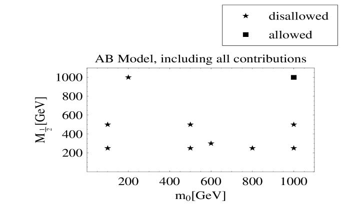
In Table 1 we give the branching ratio of the process $\mu\to e\gamma$ and the individual contributions from the sources $\hat{\delta}^{ji}_{LL},\ \delta^{ji}_{LR,RL}$ and $(\delta^{ji}_{LL})^{RHN}$ (see Eqs. (71), (80) and (81)) evaluated in the SO(10)-BPW model, with some sample choices of (m_o, m_1/2). For these calculations, to be concrete, we set ln$\left(\frac{M^{*}}{M_{GUT}}\right)$ = 1, i.e. $M^{*}\approx 3M_{GUT}$, $\tan\beta=10$, $A_{o}$( at M^∗) = 0 and $\mu>0$. In the BPW model, for concreteness, the RH neutrino masses are taken to be M${}_{R_{1}}=10^{10}$ GeV, M${}_{R_{2}}=10^{12}$ GeV and M${}_{R_{3}}=5\times 10^{14}$ GeV (see Eq. (2)). For the masses of the right-handed neutrinos in the AB model, we set M${}_{R_{1}}=7.5\times 10^{8}$ GeV, M${}_{R_{2}}=7.5\times 10^{8}$ GeV and M${}_{R_{3}}=2.6\times 10^{14}$ GeV corresponding to $a=c=4$ and $b=6$ in Eq. (65). (The results on the rate of $\mu\to e\gamma$, presented in the following table do not change very much for other ($\mathcal{O}(1)$) values of $a,\ b$ and $c$.). It should be noted that the corresponding values for the G(224)-BPW model are smaller than those for the SO(10)-BPW model approximately by a factor of 4 to 6 in the rate, provided $\ln(M^{*}/M_{GUT})$ is the same in both cases (see comments below Eqs. (70) and (75)). A pictorial representation of these results is depicted in Figs. 1 and 2.

$(m_{o},~{}m_{1/2})$(GeV)	$A_{L}^{(1)}(\hat{\delta}_{LL})$	$A_{L}^{(2)}(\delta_{LR})$	$A_{R}(\delta_{RL})$	$A_{L}^{(3)}((\delta_{LL})^{RHN})$	Br($\mu\to e\gamma$)
(100, 250) BPW	$-1.2\times 10^{-10}$	$4.5\times 10^{-13}$	$-7.2\times 10^{-11}$	$3.7\times 10^{-14}$	$1.3\times 10^{-7}$
(100, 250) AB	$-8.5\times 10^{-11}$	$1.9\times 10^{-12}$	$-6.4\times 10^{-11}$	$1.3\times 10^{-12}$	$8.0\times 10^{-8}$
(500, 250) BPW	$-1.9\times 10^{-12}$	$1.0\times 10^{-12}$	$-1.6\times 10^{-12}$	$8.5\times 10^{-14}$	$2.2\times 10^{-11}$
(500, 250) AB	$-1.4\times 10^{-12}$	$4.4\times 10^{-12}$	$-1.4\times 10^{-12}$	$2.9\times 10^{-12}$	$2.6\times 10^{-10}$
(800, 250) BPW	$-3.5\times 10^{-13}$	$6.1\times 10^{-13}$	$-2.9\times 10^{-13}$	$4.9\times 10^{-14}$	$\mathbf{1.3\times 10^{-12}}$
(800, 250) AB	$-2.6\times 10^{-13}$	$2.5\times 10^{-12}$	$-2.6\times 10^{-13}$	$1.7\times 10^{-12}$	$1.1\times 10^{-10}$
(1000, 250) BPW	$-1.5\times 10^{-13}$	$4.3\times 10^{-13}$	$-1.2\times 10^{-13}$	$3.5\times 10^{-14}$	$\mathbf{8.1\times 10^{-13}}$
(1000, 250) AB	$-1.1\times 10^{-13}$	$1.8\times 10^{-12}$	$-1.1\times 10^{-13}$	$1.2\times 10^{-12}$	$5.9\times 10^{-11}$
(600, 300) BPW	$-1.3\times 10^{-12}$	$7.2\times 10^{-13}$	$-1.1\times 10^{-12}$	$5.9\times 10^{-14}$	$\mathbf{1.1\times 10^{-11}}$
(600, 300) AB	$-9.8\times 10^{-13}$	$3.0\times 10^{-12}$	$-9.7\times 10^{-13}$	$2.0\times 10^{-12}$	$1.3\times 10^{-10}$
(100, 500) BPW	$-5.4\times 10^{-11}$	$3.5\times 10^{-14}$	$-2.8\times 10^{-11}$	$2.8\times 10^{-15}$	$2.6\times 10^{-8}$
(100, 500) AB	$-4.0\times 10^{-11}$	$1.5\times 10^{-13}$	$-2.5\times 10^{-11}$	$9.7\times 10^{-14}$	$1.6\times 10^{-8}$
(500, 500) BPW	$-4.3\times 10^{-12}$	$3.1\times 10^{-13}$	$-3.3\times 10^{-12}$	$2.5\times 10^{-14}$	$1.9\times 10^{-10}$
(500, 500) AB	$-3.2\times 10^{-12}$	$1.3\times 10^{-12}$	$-3.0\times 10^{-12}$	$8.6\times 10^{-13}$	$7.5\times 10^{-11}$
(1000, 500) BPW	$-4.8\times 10^{-13}$	$2.6\times 10^{-13}$	$-3.9\times 10^{-13}$	$2.1\times 10^{-14}$	$\mathbf{1.4\times 10^{-12}}$
(1000, 500) AB	$-3.5\times 10^{-13}$	$1.1\times 10^{-12}$	$-3.5\times 10^{-13}$	$7.3\times 10^{-13}$	$1.6\times 10^{-11}$
(200, 1000) BPW	$-1.3\times 10^{-11}$	$8.8\times 10^{-15}$	$-7.1\times 10^{-12}$	$7.2\times 10^{-16}$	$1.6\times 10^{-9}$
(200, 1000) AB	$-9.9\times 10^{-12}$	$3.7\times 10^{-14}$	$-6.4\times 10^{-12}$	$2.4\times 10^{-14}$	$1.0\times 10^{-9}$
(1000, 1000) BPW	$-1.1\times 10^{-12}$	$7.7\times 10^{-14}$	$-8.3\times 10^{-13}$	$6.3\times 10^{-15}$	$\mathbf{1.2\times 10^{-11}}$
(1000, 1000) AB	$-7.9\times 10^{-13}$	$3.2\times 10^{-13}$	$-7.4\times 10^{-13}$	$2.2\times 10^{-13}$	$\mathbf{4.7\times 10^{-12}}$

Table 1. Comparison between the AB and the BPW models of the various contributions to the amplitude and of the branching ratio for $\mu\to e\gamma$ for the case of SO(10). Each of the entries for the amplitudes should be multiplied by a common factor a_o. Imaginary parts being small are not shown. Only the cases shown in bold typeface are in accord with experimental bounds; the other ones are excluded. The first three columns denote contributions to the amplitude from post-GUT physics arising from the regime of $M^{*}\to M_{GUT}$ (see Eqs. (71)–(80)), where for concreteness we have chosen $\ln(M^{*}/M_{GUT})=1$. The fifth column denotes the contribution from the right-handed neutrinos (RHN). Note that the entries corresponding to the RHN-contribution are much larger in the AB-model than those in the BPW-model; this is precisely because the AB-model is lopsided while the BPW model is hierarchical (see text). Note that for the BPW model, the post-GUT contribution far dominates over the RHN-contribution while for the AB model they are comparable. The last column gives the branching ratio of $\mu\to e\gamma$ including contributions from all four columns. The net result is that the AB model is compatible with the empirical limit on $\mu\to e\gamma$ only for rather heavy SUSY spectrum like $(m_{o},~{}m_{1/2})\buildrel>\over{{}_{\sim}}(1000,~{}1000)$ GeV, whereas the BPW is fully compatible with lighter SUSY spectrum like $(m_{o},~{}m_{1/2})\sim(600,~{}300)$ GeV (see text) for the case of SO(10), and $(m_{o},~{}m_{1/2})\sim(400,~{}250)$ GeV for G(224). These results are depicted graphically in Figs. 1 and 2.

Before discussing the features of this table, it is worth noting some distinguishing features of the BPW and the AB models. As can be inferred from Eqs. (75) and (79), for a given $m_{o}$, the post-GUT contribution for both the BPW and the AB models increases with increasing $m_{1/2}$ primarily due to the A-term contribution. It turns out that for $m_{1/2}\buildrel>\over{{}_{\sim}}300$ GeV, this contribution becomes so large that Br($\mu\to e\gamma$) exceeds the experimental limit, unless one chooses $m_{o}\buildrel>\over{{}_{\sim}}1000$ GeV, so that the rate is suppressed due to large slepton masses. This effect applies to both models.

For the hierarchical BPW model, however, it turns out that the RHN contribution is strongly suppressed both relative to that in the lopsided AB-model; and also relative to the post-GUT contributions (see discussion below). As a result the dominant contribution for the BPW model comes only from post-GUT physics, which decreases with decreasing $m_{1/2}$ for a fixed $m_{o}$. Such a dependence on $m_{1/2}$ is not so striking, however, for the AB model because in this case, owing to the lopsided structure, the RHN contribution (which is not so sensitive to $m_{1/2}$) is rather important and is comparable to the post-GUT contribution.

Tables 1 and 2 bring out some very interesting distinctions between the two models:

(1) The experimental limit on $\mu\to e\gamma$ is given by: Br($\mu\to e\gamma)<1.2\times 10^{-11}$ [35]. This means that for the case of the AB model, with dominant contribution coming not only from post-GUT physics but also from the RHN contribution, only rather heavy SUSY spectrum, $(m_{o},\ m_{1/2})\buildrel>\over{{}_{\sim}}(1000,\ 1000)$ GeV, is allowed. The BPW-model, on the other hand, allows for relatively low $m_{1/2}$ ($\buildrel<\over{{}_{\sim}}300$ GeV), with moderate to heavy $m_{o}$, which can be as low as about 600 GeV with $m_{1/2}\leq 300$ GeV. As a result, whereas the AB model is consistent with $\mu\to e\gamma$ only for rather heavy sleptons ($\buildrel>\over{{}_{\sim}}1200$ GeV) and heavy squarks ($\buildrel>\over{{}_{\sim}}$ 2.8 TeV), the BPW model is fully compatible with much lighter slepton masses $\sim 600$ GeV, with squarks being 800 GeV to 1 TeV. These results hold for the case od SO(10). For the G(224) case the BPW model would be consistent with the experimental limit on the rate of $\mu\to e\gamma$ for even lighter SUSY spectrum including values of $(m_{o},~{}m_{1/2})\approx(400,~{}250)$ GeV, which corresponds to $m_{\tilde{q}}\sim 780$ GeV and $m_{\tilde{l}}\sim 440$ GeV.

(2) From the point of view of forthcoming experiments we also note that $\mu\to e\gamma$ for the BPW case, ought to seen with an improvement in the current limit by a factor of 10–50. For the AB case, even with a rather heavy SUSY spectrum ($(m_{o},\ m_{1/2})\buildrel>\over{{}_{\sim}}(1000,\ 1000)$ GeV), $\mu\to e\gamma$ should be seen with an improvement by a factor of only 3–5. Such experiments are being planned at the MEG experiment at PSI [32]

(3) As has been noted earlier in [33] and more recently in [17], the contribution to $A_{L}(\mu\to e\gamma)$ due to RH neutrinos in the BPW model is approximately proportional to $\eta-\sigma\approx 0.041$, which is naturally small because the entries $\eta$ and $\sigma$ are of $\mathcal{O}(1/10)$ in magnitude due to the hierarchical structure. In the AB-model on the other hand, this contribution is proportional to $\tilde{\sigma}+2\tilde{\epsilon}/3\approx 1.8$. Thus we expect that in amplitude, the RHN contribution in the BPW model is smaller by about a factor of 40 than that in the AB model. This has two consequences:

(a) First, there is a dramatic difference between the two models which becomes especially prominent if one drops the post-GUT contribution, that amounts to setting $M^{*}=M_{GUT}$. In this case the contribution to $(\mu\to e\gamma)$ comes entirely from the RHN contribution. In this case the branching ratio of $(\mu\to e\gamma)$ in the two models differs by a factor of about $(40)^{2}\sim\mathcal{O}(10^{3})$ as depicted in table 2.

$(m_{o},~{}m_{1/2})$(GeV)	Br$(\mu\to e\gamma)_{AB}^{RHN}$	Br$(\mu\to e\gamma)_{BPW}^{RHN}$
(100, 250)	$1.2\times 10^{-11}$	$9.7\times 10^{-15}$
(800, 250)	$2.1\times 10^{-11}$	$1.7\times 10^{-14}$
(600, 300)	$2.8\times 10^{-11}$	$2.5\times 10^{-14}$
(500, 500)	$5.3\times 10^{-12}$	$4.4\times 10^{-15}$
(1000, 1000)	$3.4\times 10^{-13}$	$2.8\times 10^{-16}$

Table 2. Branching ratio for $(\mu\to e\gamma)$ based only on the RHN contribution (this corresponds to setting $M^{*}=M_{GUT}$) for the AB and BPW models for different choices of $(m_{o},~{}m_{1/2})$.

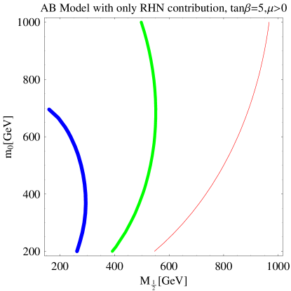
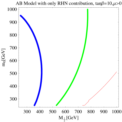
It can be seen from table 2 that with only the RHN contribution (which would be the total contribution if $M^{*}=M_{GUT}$), the AB model is consistent with the limit on $\mu\to e\gamma$ for light SUSY spectrum, e.g. for $(m_{o},~{}m_{1/2})=(100,250)$ GeV. A similar analysis for the AB model was done in Ref. [26] (including the RHN contribution only), and our results agree with those of Ref. [26]. One may expect that for the same value of $m_{1/2}$, increasing $m_{o}$ would result in decreasing the branching ratio. For example, from Eq. (81), one may expect the rate for $\mu\to e\gamma$ to be proportional to $(m_{o}^{2}/m_{\tilde{l}}^{4})^{2}\sim 1/m_{o}^{4}$. However, the associated loop function (see e.g. Ref. [34]) alters the dependence on $(m_{o},~{}m_{1/2})$ drastically; it increases with increasing $m_{o}$, for fixed $m_{1/2}$. The net result of these two effects is that for the same $m_{1/2}$, a low $m_{o}\sim 100$ GeV and a high $m_{o}\sim 1000$ GeV, give nearly the same value of the branching ratio for $\mu\to e\gamma$ with the inclusion of only the RH neutrino contribution (see Fig. 3) . This can also be seen in the results of Ref. [26] which analyzes the AB model. The RHN contribution in the case of the BPW model is extremely small because of its hierarchical structure, as explained above.

Of course, in the context of supersymmetry breaking as in mSUGRA or gaugino-mediation, we expect $M^{*}>M_{GUT}$, thus post-GUT contributions should be included at least in these cases. With the inclusion of post-GUT physics,as mentioned above, the AB model is consistent with the experimental limit on $\mu\to e\gamma$, only for very heavy SUSY spectrum with $(m_{o},\ m_{1/2})\buildrel>\over{{}_{\sim}}(1000,\ 1000)$ GeV, i.e. $m_{\tilde{l}}\buildrel>\over{{}_{\sim}}1200$ GeV and $m_{\tilde{q}}\buildrel>\over{{}_{\sim}}2.8$ TeV; whereas the BPW model is fully compatible with the empirical limit for significantly lower values of $(m_{o},\ m_{1/2})\sim(600,\ 300)$ GeV, i.e. $m_{\tilde{l}}\sim 600$ GeV and $m_{\tilde{q}}\sim 1$ TeV (see table 1).

(b) Second, it was shown in Ref. [17] that the P-odd asymmetry parameter for the process $(\mu^{+}\to e^{+}\gamma)$ defined as $\mathcal{A}(\mu^{+}\rightarrow e^{+}\gamma)=(|A_{L}|^{2}-|A_{R}|^{2})/(|A_{L}|^{2}+|A_{R}|^{2})$ (where $|A_{L}|=|A_{L}^{(1)}(\hat{\delta}_{LL})+A_{L}^{(2)}(\delta_{LR})+A_{L}^{(3)}|)$, is typically negative for the BPW model except for cases with very large $m_{1/2}$ e.g. $(m_{o},\ m_{1/2})=(1000,\ 1000)$ or $(500,\ 500)$ GeV. For the AB-case, due to the large RHN contribution, $|A_{L}|>|A_{R}|$ and therefore the P-odd asymmetry parameter ${\mathcal{A}}$ would typically be positive. Thus the determination of ${\mathcal{A}}$ in future experiments can help distinguish between the BPW and the AB models.

For the sake of completeness, we give the branching ratios of the processes $\tau\to\mu\gamma$ and $\tau\to e\gamma$ calculated in the two models in table 3.

($m_{o},\ m_{1/2}$)(GeV)	AB-model		BPW-model
	Br($\tau\to\mu\gamma$)	Br($\tau\to e\gamma$)	Br($\tau\to\mu\gamma$)	Br($\tau\to e\gamma$)
(100, 250)	$2.9\times 10^{-9}$	$3.8\times 10^{-11}$	2.6$\times 10^{-7}$	1.6$\times 10^{-9}$
(800, 250)	$1.0\times 10^{-8}$	$4.5\times 10^{-11}$	1.6$\times 10^{-9}$	6.8$\times 10^{-12}$
(600, 300)	$1.4\times 10^{-8}$	$6.4\times 10^{-11}$	2.1$\times 10^{-9}$	8.4$\times 10^{-12}$
(500, 500)	$2.4\times 10^{-9}$	$1.0\times 10^{-11}$	3.9$\times 10^{-10}$	1.8$\times 10^{-12}$
(1000, 1000)	$1.5\times 10^{-10}$	$6.5\times 10^{-13}$	2.5$\times 10^{-11}$	1.1$\times 10^{-13}$

Table 3. Branching ratios for $(\tau\to\mu\gamma)$ and $(\tau\to e\gamma)$ evaluated in the two models for the case of SO(10), for some sample choices of $(m_{o},~{}m_{1/2})$. We have set $\tan\beta=10,\ \mu>0$ and ln$\left(\frac{M^{*}}{M_{GUT}}\right)$ = 1.

From table 3 we see that the predictions for the branching ratios for $(\tau\to\mu\gamma)$ and $(\tau\to e\gamma)$ in either model are well below the current experimental limits. The process $(\tau\to\mu\gamma)$ can be probed at BABAR and BELLE or at LHC in the forthcoming experiments; $(\tau\to e\gamma)$ seems to be out of the reach of the upcoming experiments.

In the following section we turn to CP violation in the two models.

5 Results on Fermion Masses, CKM Elements and CP Violation

CP violation in the BPW model was studied in detail in Ref. [16]. We will recapitulate some of those results and do a comparative study with the AB model. For any choice of the parameters in the mass matrices ($\eta,\ \sigma,\ \epsilon$ etc. for the BPW case, and $\tilde{\sigma},\ \tilde{\epsilon}$ etc. for the AB case), one gets the SO(10)-model based values of $\rho_{W}$ and $\eta_{W}$, which generically can differ widely from the SM-based phenomenological values. We denote the former by $(\rho^{\prime}_{W})_{BPW,AB}$ and $(\eta^{\prime}_{W})_{BPW,AB}$ and the corresponding contributions from the SM-interactions (based on $\rho^{\prime}_{W}$ and $\eta^{\prime}_{W}$) by SM^′. In our calculations we include both the SM^′ contribution and the SUSY contributions involving the sfermion $(mass)^{2}$-parameters($\delta^{ij}_{LL,RR,LR})$ which are in general CP violating. These parameters are completely determined in each of the two models for a given choice of flavor preserving SUSY-parameters (i.e. $m_{o},\ m_{1/2},\ \mu$, and $\tan\beta$; we set $A_{o}$ = 0 at $M^{*}$). Using the fits given in Eqs. (44) and (69), we get the following values for the CKM elements and fermion masses using $m_{t}(m_{t})=167\ GeV$ and $m_{\tau}(m_{\tau})=1.777\ GeV$ as inputs:
BPW:

$$\begin{array}[]{l}\ \ \ \ ((V_{us},\ V_{cb},\ |V_{ub}|,\ |V_{td}|)(\leq m_{Z}))_{BPW}\approx(0.2250,\ 0.0412,\ 0.0037,\ 0.0086)\\ \begin{array}[]{l}\ \ \ (\bar{\rho}^{\prime}_{W})_{BPW}=0.150,\quad(\bar{\eta}^{\prime}_{W})_{BPW}=0.374\\ \begin{array}[]{l}\ \ (m_{b}(m_{b}),\ m_{c}(m_{c}))\approx(4.97,\ 1.32)\ GeV\\ \begin{array}[]{l}\ (m_{s}(1GeV),\ m_{\mu})\approx(101,\ 109)\ MeV\\ \begin{array}[]{l}(m_{u}^{\circ}(1GeV),\ m_{d}^{\circ}(1GeV),\ m_{e}^{\circ})\approx(10.1,\ 3.7,\ 0.13)\ MeV\end{array}\end{array}\end{array}\end{array}\end{array}$$ (93)

AB:

$$\begin{array}[]{l}\ \ \ \ ((V_{us},\ V_{cb},\ |V_{ub}|,\ |V_{td}|)(\leq m_{Z}))_{AB}\approx(0.220,\ 0.041,\ 0.0032,\ 0.0081)\\ \begin{array}[]{l}\ \ \ (\bar{\rho}^{\prime}_{W})_{AB}=0.148,\quad(\bar{\eta}^{\prime}_{W})_{AB}=0.309\\ \begin{array}[]{l}\ \ (m_{b}(m_{b}),\ m_{c}(m_{c}))\approx(4.97,\ 1.15)\ GeV\\ \begin{array}[]{l}\ (m_{s}(1GeV),\ m_{\mu})\approx(177,\ 106)\ MeV\\ \begin{array}[]{l}(m_{u}^{\circ}(1GeV),\ m_{d}^{\circ}(1GeV),\ m_{e}^{\circ})\approx(3.2,\ 8.5,\ 0.56)\ MeV\end{array}\end{array}\end{array}\end{array}\end{array}$$ (103)

The predictions of both models for the CKM elements are in good agreement with the measured values, and $(\bar{\rho}^{\prime}_{W})$ and $\bar{\eta}^{\prime}_{W})$ are close to the SM values in each case. It was remarked in Ref. [16] that for the BPW model, the masses of the light fermions (u, d and e) can be corrected by allowing for $\mathcal{O}(10^{-4}-10^{-5})$ “11” entries in the mass matrices which can arise naturally through higher dimensional operators. Such small entries will not alter the predictions for the CKM mixings. For the AB model, the masses of the bottom and strange quarks have been lowered by the gluino loop contributions from 5.12 GeV and 183 MeV to 4.97 GeV and 177 MeV respectively. Thus from Eqs. (93) and (103), we see that both models are capable of yielding the gross pattern of fermion masses and especially the CKM mixings in good accord with observations; at the same time $(\bar{\rho}^{\prime}_{W})$ and $\bar{\eta}^{\prime}_{W})$ are close to the phenomenological SM values.

We now present some results on CP violation. We include both the SM^′ and the SUSY contributions in obtaining the total contributions (denoted by “Tot”). The SUSY contribution is calculated using the squark mixing elements, $\delta^{ij}_{LL,RR,LR}$, which are completely determined in both models for any given choice of the SUSY breaking parameters $m_{o},\ m_{1/2},\ A_{o},\tan\beta$ and $sgn(\mu)$. As emphasized earlier, in our calculations, the $\delta^{ij}s$ include contributions from both post-GUT physics as well as those coming from RG running in MSSM below the GUT scale. (For details, see Ref. [16]). We set $A_{o}=0$ for concreteness, as before. Listed below in Table 4 are the results on CP and flavor violations in the $\rm{K}^{\circ}-\overline{\rm{K}^{\circ}}$ and $\rm{B_{d}}^{\circ}-\overline{\rm{B_{d}}^{\circ}}$ systems for the two models. For these calculations we set $\ln(M^{*}/M_{GUT})=1$.

$(m_{o},~{}m_{1/2})$(GeV)	$\Delta m_{K}^{s.d.}$(GeV)	$\epsilon_{K}(SM^{\prime})$	$\epsilon_{K}(Tot)$	$\Delta m_{B_{d}}$ (GeV)	$S_{\psi K_{S}}$
	Tot $\approx$ SM′			Tot $\approx$ SM′	Tot $\approx$ SM′
(300, 300) BPW	$2.9\times 10^{-15}$	$2.8\times 10^{-3}$	$2.6\times 10^{-3}$	$3.5\times 10^{-13}$	$0.73$
(300, 300) AB	$2.8\times 10^{-15}$	$2.2\times 10^{-3}$	$2.2\times 10^{-3}$	$3.1\times 10^{-13}$	$0.66$
(600, 300) BPW	$2.9\times 10^{-15}$	$2.8\times 10^{-3}$	$2.0\times 10^{-3}$	$3.6\times 10^{-13}$	$0.73$
(600, 300) AB	$2.8\times 10^{-15}$	$2.2\times 10^{-3}$	$1.4\times 10^{-3}$	$3.1\times 10^{-13}$	$0.66$
(1000, 250) BPW	$2.9\times 10^{-15}$	$2.8\times 10^{-3}$	$1.4\times 10^{-3}$	$3.6\times 10^{-13}$	$0.74$
(1000, 250) AB	$2.8\times 10^{-15}$	$2.2\times 10^{-3}$	$-4.0\times 10^{-3}$	$3.13\times 10^{-13}$	$0.656$
(1000, 500) BPW	$2.9\times 10^{-15}$	$2.83\times 10^{-3}$	$2.6\times 10^{-3}$	$3.6\times 10^{-13}$	$0.73$
(1000, 500) AB	$2.8\times 10^{-15}$	$2.2\times 10^{-3}$	$2.0\times 10^{-3}$	$3.1\times 10^{-13}$	$0.66$
(1000, 1000) BPW	$2.9\times 10^{-15}$	$2.8\times 10^{-3}$	$2.9\times 10^{-3}$	$3.5\times 10^{-13}$	$0.72$
(1000, 1000) AB	$2.8\times 10^{-15}$	$2.2\times 10^{-3}$	$2.3\times 10^{-3}$	$3.1\times 10^{-13}$	$0.66$

Table 4. CP violation in the $K^{\circ}-\overline{K^{\circ}}$ and $B_{d}-\overline{B_{d}}$ systems as predicted in the BPW and the AB models for some sample choices of $(m_{o},\ m_{1/2})$ and a generic fit of parameters (see Eq.(44) for the BPW case and Eq. (69) for the AB case). The superscript s.d. on $\Delta m_{K}$ denotes the short distance contribution. The predictions in either model are in good agreement with experimental data for most of the cases displayed above, especially given the uncertainties in the matrix elements (see text). It may be noted that values of $S(B_{d}\rightarrow J/\psi K_{S})$ as high as 0.74 in the AB model, and as low as 0.65 in the BPW model, can be achieved by varying the fit.

In obtaining the entries for the $K$-system we have used central values of the matrix element $\hat{B}_{K}$ and the loop functions $\eta_{i}$ (see Refs. [36, 37] for definitions and values) characterizing short distance QCD effects - i.e. $\hat{B}_{K}=0.86\pm 0.13,\ f_{K}=159\ MeV,\ \eta_{1}=1.38\pm 0.20$, $\eta_{2}=0.57\pm 0.01$ and $\eta_{3}=0.47\pm 0.04$. For the $B$-system we use the central values of the unquenched lattice results: $f_{B_{d}}\sqrt{\hat{B}_{B_{d}}}=215(11)(^{+0}_{-23})(15)\ MeV$ and $f_{B_{s}}\sqrt{\hat{B}_{B_{s}}}=245(10)(^{+3}_{-2})(^{+7}_{-0})\ MeV$ [38]. Note that the uncertainties in some of these hadronic parameters are in the range of 15%; thus the predictions of the two SO(10) models as well as those of the SM would be uncertain at present to the same extent.

Some points of distinctions and similarities between the two models are listed below.

(1) First note that the data point $(m_{o},\ m_{1/2})$ = (300, 300) GeV displayed above, though consistent with CP violation, gives too large a value for Br($\mu\to e\gamma$) for both BPW and AB models. All other cases shown in table 4 are consistent with the experimental limit on $\mu\to e\gamma$ for the BPW model. For the AB model on the other hand, as may be inferred from table 1, the choice $(m_{o},\ m_{1/2})$ = (1000, 1000) GeV is the only case that is consistent with the limit on $\mu\to e\gamma$ (see table 1). It is to be noted that for this case the squark masses are extremely high ($\sim 2.8$ TeV), and therefore, in the AB model, once the $\mu\to e\gamma$ constraint is satisfied, the SUSY contributions are strongly suppressed for all four entities: $\Delta m_{K},\ \epsilon_{K},\ \Delta m_{B_{d}}$ and $S(B_{d}\rightarrow J/\psi K_{S})$.

(2) For the BPW model on the other hand, there are good regions of parameter space allowed by the limit on the rate of $\mu\to e\gamma$ (e.g. $(m_{o},~{}m_{1/2})=(600,~{}300)$ GeV), which are also in accord with $\epsilon_{K}$. The SUSY contribution to $\epsilon_{K}$ for these cases is sizable ($\sim 20-30\%$) and negative, as desired.

(3) We have exhibited the case $(m_{o},\ m_{1/2})$ = (1000, 250) GeV to illustrate that this case does not work for either model as it gives too low a value for $\epsilon_{K}$ in the BPW model, and a negative value in the AB model. In this case the SUSY contribution, which is negative, is sizable because of the associated loop functions which are increasing functions of $(m_{sq}^{2}/m_{\tilde{g}}^{2})$.

(4) The predictions regarding $\Delta m_{K}$, $\Delta m_{B_{d}}$ and $S(B_{d}\rightarrow J/\psi K_{S})$ are very similar in both the models, i.e they are both close to the SM value.

(5) As noted above, there are differences between the predictions of the BPW vs. the AB models for $\epsilon_{K}$ for a given $(m_{o},\ m_{1/2})$. With uncertainties in $\hat{B}_{K}$ and the SUSY spectrum, $\epsilon_{K}$ cannot, however, be used at present to choose between the two models, but if $(m_{o},\ m_{1/2})$ get determined (e.g. following SUSY searches at the LHC) and $\hat{B}_{K}$ is more precisely known through improved lattice calculations, $\epsilon_{K}$ can indeed distinguish between the BPW and the AB models, as also between SO(10) and G(224) models (for details on this see Ref. [16]). This distinction can be sharpened especially by searches for $\mu\to e\gamma$.

(6) $B_{d}\rightarrow\phi K_{S},\ \Delta m_{B_{s}}$: Including the SM^′ and SUSY contributions to the decay $B_{d}\rightarrow\phi K_{S}$, we get the following results for the CP violating asymmetry parameter S($B_{d}\rightarrow\phi K_{S}$) in the two models:

$$\begin{array}[]{l}{\rm\bf BPW:\ \ }S(B_{d}\rightarrow\phi K_{S})\approx+0.65-0.74~{}.\\ \begin{array}[]{l}{\rm\bf\ \ AB:\ \ }S(B_{d}\rightarrow\phi K_{S})\approx+0.61-0.65~{}.\\ \end{array}\end{array}$$ (107)

The values displayed above for the AB model are calculated for the fit given in Eq. (69). For variant fits in the AB model, values as high as S($B_{d}\rightarrow\phi K_{S})\approx$ 0.7 may be obtained. The SUSY contribution to the amplitude for the decay $B_{d}\rightarrow\phi K_{S}$ in the BPW model is only of order 1%, whereas in the AB model it is nearly 5% for light SUSY spectrum ($(m_{o},\ m_{1/2})\sim(300,300)$ GeV) and about 1% for large $(m_{o},\ m_{1/2})(\sim(1000,500)$ GeV). The main point to note is that in both models S($B_{d}\rightarrow\phi K_{S}$) is positive in sign and close to the SM prediction. The current experimental values for the asymmetry parameter are $S(B_{d}\rightarrow\phi K_{S})=(+0.50\pm 0.25^{+0.07}_{-0.04})_{BaBar};(+0.06\pm 0.33\pm 0.09)_{BELLE}$ [39]. While the central values of these two measurements are very different, the errors on them are large. It will thus be extremely interesting from the viewpoint of the two frameworks presented here to see whether the true value of $S(B_{d}\rightarrow\phi K_{S})$ will turn out to be close to the SM-prediction or not.

Including SUSY contributions to $B_{s}-\overline{B_{s}}$ mixing coming from $\delta^{23}_{LL,RR,LR,RL}$ insertions we get:

$$\begin{array}[]{l}{\bf BPW:\ \ }\Delta m_{B_{s}}(Tot\approx SM^{\prime})\approx{\bf 17.3}\ ps^{-1}\bigl{(}\frac{f_{B_{s}}\sqrt{\hat{B}_{B_{s}}}}{245MeV}\bigr{)}^{2}~{}.\\ \begin{array}[]{l}{\bf\ \ AB:\ \ }\Delta m_{B_{s}}(Tot\approx SM^{\prime})\approx{\bf 16.6}\ ps^{-1}\bigl{(}\frac{f_{B_{s}}\sqrt{\hat{B}_{B_{s}}}}{245MeV}\bigr{)}^{2}~{}.\\ \end{array}\end{array}$$ (111)

Both predictions are compatible with the present lower limit on $\Delta m_{B_{s}}\buildrel>\over{{}_{\sim}}14.4ps^{-1}$ [41].

(7) Contribution of the A term to $\epsilon^{\prime}_{K}$: Direct CP violation in $K_{L}\rightarrow\pi\pi$ receives a new contribution from the chromomagnetic operator $Q^{-}_{g}=(g/16\pi^{2})(\bar{s}_{L}\sigma^{\mu\nu}t^{a}d_{R}-\bar{s}_{R}\sigma^{\mu\nu}t^{a}d_{L})G^{a}_{\mu\nu}$, which is induced by the gluino penguin diagram. This contribution is proportional to $Im[(\delta^{d}_{LR})_{21}-(\delta^{d}_{LR})_{12}^{*}]$, which is known in both models (see Eqs. (75) and (79)). Following Refs. [42] and [43], one obtains:

$$Re(\epsilon^{\prime}/\epsilon)_{\tilde{g}}\approx 91\ B_{G}\bigl{(}\frac{110~{}MeV}{m_{s}+m_{d}}\bigr{)}\bigl{(}\frac{500~{}GeV}{m_{\tilde{g}}}\bigr{)}~{}Im[(\delta^{d}_{LR})_{21}-(\delta^{d}_{LR})_{12}^{*}]$$ (112)

where $B_{G}$ is the relevant hadronic matrix element. Model-dependent considerations (allowing for $m_{K}^{2}/m_{\pi}^{2}$ corrections) indicate that $B_{G}\approx 1-4$, and that it is positive [42]. Putting in the values of $\delta^{d}_{LR})_{12,21}$ obtained in each model with ($m_{o},\ m_{1/2}$) = (a) (600, 300) GeV, and (b) (1000, 1000) GeV, we get:

$$\begin{array}[]{l}{\bf BPW:\ \ \ }Re(\epsilon^{\prime}/\epsilon)_{\tilde{g}}\approx+(3.7\times 10^{-4})(B_{G}/4)(10/\tan\beta)\quad Case\ (a)~{}.\\ \begin{array}[]{l}~{}~{}~{}~{}~{}~{}~{}~{}~{}~{}~{}~{}~{}~{}~{}~{}~{}~{}~{}~{}~{}~{}~{}~{}\approx+(4.5\times 10^{-5})(B_{G}/4)(10/\tan\beta)\quad Case\ (b)~{}.\\ \begin{array}[]{l}{\bf\ \ AB:\ \ }Re(\epsilon^{\prime}/\epsilon)_{\tilde{g}}\approx-(3.7\times 10^{-5})(B_{G}/4)(10/\tan\beta)\quad Case\ (a)~{}.\\ \begin{array}[]{l}~{}~{}~{}~{}~{}~{}~{}~{}~{}~{}~{}~{}~{}~{}~{}~{}~{}~{}~{}~{}~{}\approx+(4.5\times 10^{-6})(B_{G}/4)(10/\tan\beta)\quad Case\ (b)~{}.\\ \end{array}\end{array}\end{array}\end{array}$$ (120)

Whereas both cases (a) and (b) are consistent with the limit on $\mu\to e\gamma$ for the BPW model, only case (b) is in accord with $\mu\to e\gamma$ for the AB model. The observed value of $Re(\epsilon^{\prime}/\epsilon)_{obs}$ is given by $Re(\epsilon^{\prime}/\epsilon)_{obs}=(17\pm 2)\times 10^{-4}$ [44]. At present the theoretical status of SM contribution to $Re(\epsilon^{\prime}/\epsilon)$ is rather uncertain. For instance, the results of Ref. [45] and [46] based on quenched lattice calculations in the lowest order chiral perturbation theory suggest negative central values for $Re(\epsilon^{\prime}/\epsilon)$. (To be specific Ref. [45] yields $Re(\epsilon^{\prime}/\epsilon)_{SM}=(-4.0\pm 2.3)\times 10^{-4}$, the errors being statistical only.) On the other hand, using methods of partial quenching [47] and staggered fermions, positive values of $Re(\epsilon^{\prime}/\epsilon)$ in the range of about $(3-13)\times 10^{-4}$ are obtained in [48]. In addition, a recent non-lattice calculation based on next-to-leading order chiral perturbation theory yields $Re(\epsilon^{\prime}/\epsilon)_{SM}=(19\pm 2^{+9}_{-6}\pm 6)\times 10^{-4}$ [49]. The systematic errors in these calculations are at present hard to estimate. The point to note here is that the BPW model predicts a relatively large and positive SUSY contribution to $Re(\epsilon^{\prime}/\epsilon)$, especially for case (a), which can eventually be relevant to a full understanding of the value of $\epsilon^{\prime}_{K}$, whereas this contribution in the AB model is rather small for both cases. Better lattice calculations can hopefully reveal whether a large contribution, as in the BPW model, is required or not.

(8) EDM of the neutron and the electron: RG-induced $A$-terms of the model generate chirality-flipping sfermion mixing terms $(\delta_{LR}^{d,u,l})_{ij}$, whose magnitudes and phases are predictable in the two models (see Eq. (80)), for a given choice of the universal SUSY-parameters ($m_{o},\ m_{1/2},\ and\ \tan\beta$). These contribute to the EDM’s of the quarks and the electron by utilizing dominantly the gluino and the neutralino loops respectively. We will approximate the latter by using the bino-loop. These contributions are given by (see e.g. [50]):

$$\begin{array}[]{c}(d_{d},d_{u})_{A_{ind}}=(-\frac{2}{9},\frac{4}{9})\frac{\alpha_{s}}{\pi}\ e\ \frac{m_{\tilde{g}}}{m_{sq}^{2}}f\bigl{(}\frac{m^{2}_{\tilde{g}}}{m_{sq}^{2}}\bigr{)}Im(\delta^{d,u}_{LR})_{11}\\ \begin{array}[]{cc}(d_{e})_{A_{ind}}=-\frac{1}{4\pi}\frac{\alpha_{em}}{cos^{2}\theta_{W}}\ e\ \frac{m_{\tilde{B}}}{m_{\tilde{l}}^{2}}f\bigl{(}\frac{m^{2}_{\tilde{B}}}{m_{\tilde{l}}^{2}}\bigr{)}Im(\delta^{l}_{LR})_{11}~{}.\\ \end{array}\end{array}$$ (124)

The EDM of the neutron is given by $d_{n}=\frac{1}{3}(4d_{d}-d_{u})$. The up sector being purely real implies $d_{u}=0$ in the AB model. In table 5 we give the values of $d_{n}$ and $d_{e}$ calculated in the two models for moderate and heavy SUSY spectrum and $\tan\beta=10$.

($m_{o},\ m_{1/2}$)(GeV)	AB-model		BPW-model
	$d_{n}$ (e-cm)	$d_{e}$ (e-cm)	$d_{n}$ (e-cm)	$d_{e}$ (e-cm)
I (600, 300)	$4.0\times 10^{-26}$	$1.6\times 10^{-27}$	1.1$\times 10^{-26}$	1.1$\times 10^{-29}$
II (1000, 500)	$1.4\times 10^{-26}$	$5.9\times 10^{-28}$	3.9$\times 10^{-27}$	4.1$\times 10^{-30}$
III (1000, 1000)	$5.7\times 10^{-27}$	$1.1\times 10^{-27}$	1.7$\times 10^{-27}$	7.7$\times 10^{-30}$
Expt. upper bound	$6.3\times 10^{-26}$	$4.3\times 10^{-27}$	$6.3\times 10^{-26}$	$4.3\times 10^{-27}$

Table 5. EDMs of neutron and electron calculated in the BPW and the AB models for moderate and heavy SUSY spectrum and $\tan\beta=10$ arising only from the induced A-terms. While all cases are consistent with $\mu\to e\gamma$ for the BPW model, only case III is consistent for the AB model.

From the table above, we see that while both models predict that the EDM of the neutron should be seen within an improvement by a factor of 5–10 in the current experimental limit, their predictions regarding the EDM of the electron are quite different. While the AB model predicts that the EDM of the electron should be observed with an improvement by a factor of 5–10 in the current experimental limit, the prediction of the BPW model for the EDM of the electron is that it is 2 to 3 orders of magnitude smaller than the current upper bound. These predictions are in an extremely interesting range; while future experiments on edm of the neutron can provide support for or deny both models, those on the edm of the electron can clearly distinguish between the two models.

6 Conclusions

In this paper we did a comparative study of two realistic SO(10) models: the hierarchical Babu-Pati-Wilczek (BPW) model and the lop-sided Albright-Barr (AB) model. Both models have been shown to successfully describe fermion masses, CKM mixings and neutrino oscillations. Here we compared the two models with respect to their predictions regarding CP and flavor violations in the quark and lepton sectors. CP violation is assumed to arise primarily through phases in fermion mass matrices (see e.g. Ref. [16]). For all processes we include the SM as well as SUSY contributions. For the SUSY contributions, assuming that the SUSY messenger scale $M^{*}$ lies above $M_{GUT}$ as in a mSUGRA model, we include contributions from both post-GUT physics as well as those arising due to RG running in MSSM below the GUT scale. While this has been done before for the BPW model in Refs. [16] and [17], this is the first time that flavor and CP violations have been studied in the AB model including both post-GUT and sub-GUT physics. This inclusion brings out important distinctions between the two models.

Previous works on lepton flavor violation in the AB model [20] have included only the RHN contribution associated with sub-GUT physics. It is important to note, however, that in both models the sfermion-transition elements $\delta^{ij}_{LL,RR,LR,RL}$ and the induced A parameters get fully determined for a given choice of soft SUSY-breaking parameters ($m_{o},\ m_{1/2},\ A_{o},\ \tan\beta$ and $sgn(\mu)$) and thus both contributions are well determined. Including both contributions, we find the following similarities and distinctions between the two models.

Similarities:
$\bullet$ Both models are capable of yielding values of the Wolfenstein parameters ($\rho^{\prime}_{W},\ \eta^{\prime}_{W}$) which are close to the SM values and simultaneously the right gross pattern for fermion masses, CKM elements and neutrino oscillations. For this reason, both models give the values of $\Delta m_{K},\ \Delta m_{B_{d}}$ and $S(B_{d}\to J/\psi K_{S})$ that are close to the SM predictions and agree quite well with the data. The SUSY contribution to these processes is small ($\buildrel<\over{{}_{\sim}}3\%$).
$\bullet$ For the case of $\epsilon_{K}$, it is found that for the BPW model, the SM^′ value is larger than the observed value by about 20% for central values of $\hat{B}_{K}$ and $\eta_{i}$, but the SUSY contribution is sizable and negative, so that the net value can be in good agreement with the observed value for most of the SUSY parameter space. For the AB model, for the choice of input parameters as in Eq. (69), the SM^′ value for $\epsilon_{K}$ is close to the observed value. For most of the soft-SUSY parameter space the AB model also yields $\epsilon_{K}$ in good agreement with the observed value once one allows for uncertainties in the matrix elements (see table 4).
$\bullet$ Both models predict that $S(B_{d}\to\phi K_{S})$ should be $\approx+0.65-0.74$, close to the SM predictions.
$\bullet$ The predictions regarding $\Delta m_{B_{s}}$ are similar and compatible with the experimental limit in both models.
$\bullet$ Both models predict the EDM of the neutron to be ($few\times 10^{-26}e-cm$) which should be observed with an improvement in the current limit by a factor of 5–10.

Thus a confirmation of these predictions on the edm of the neutron and $S(B_{d}\to\phi K_{S})$, would go well with the two models, but cannot distinguish between them.

Distinctions:
$\bullet$The lepton sector brings in impressive distinction between the two models through lepton flavor violation and through the EDM of the electron as noted below.
$\bullet$ The BPW model gives BR($\mu\to e\gamma$) in the range of $10^{-11}-10^{-13}$ for slepton masses $\buildrel<\over{{}_{\sim}}500$ GeV with the restriction that $m_{1/2}\buildrel<\over{{}_{\sim}}300$ GeV (see remarks below table 1). Thus it predicts that $\mu\to e\gamma$ should be seen in upcoming experiments which will have a sensitivity of $10^{-13}-10^{-14}$[32]. The contribution to $\mu\to e\gamma$ in the AB model is generically much larger than that of the BPW model. For it to be consistent with the experimental upper bound on BR($\mu\to e\gamma$), the AB model would require a rather heavy SUSY spectrum, i.e. $(m_{o},\ m_{1/2})\buildrel>\over{{}_{\sim}}(1000,\ 1000)$ GeV, i.e. $m_{\tilde{l}}\buildrel>\over{{}_{\sim}}1200$ GeV and $m_{\tilde{q}}\buildrel>\over{{}_{\sim}}2.8$ TeV. With the constraints on $(m_{o},\ m_{1/2})$ as noted above, both models predict that $\mu\to e\gamma$ should be seen with an improvement in the current limit which needs to be a factor of 10–50 for the BPW model and a factor of 3–5 for the AB model.

$\bullet$ An interesting distinction between the AB and the BPW models arises in their predictions for the EDM of the electron. The AB model give $d_{e}$ in the range $10^{-27}-10^{-28}e\ cm$ which is only a factor of 3–10 lower than the current limit. Thus the AB model predicts that the EDM of the electron should be seen in forthcoming experiments. The BPW model on the other hand predicts a value of $d_{e}$ in the range $10^{-29}-10^{-30}e\ cm$ which is about 100–1000 times lower than the current limit.

$\bullet$ In the quark sector, another interesting distinction between the two models comes from $\epsilon^{\prime}/\epsilon$. The BPW model predicts that Re($\epsilon^{\prime}/\epsilon$)${}_{SUSY}\approx+5\times 10^{-4}(B_{G}/4)(10/\tan\beta)$. Thus the BPW model predicts that SUSY will give rise to a significant positive contribution to $\epsilon^{\prime}/\epsilon$, assuming $B_{G}$ is positive [42]. The AB model gives Re($\epsilon^{\prime}/\epsilon$)${}_{SUSY}\approx-5\times 10^{-5}(B_{G}/4)(10/\tan\beta)$. Thus it predicts that the SUSY contribution is $\sim\mathcal{O}(1/10)$ the experimental value and is negative. Since the current theoretical status of the SM contribution to Re($\epsilon^{\prime}/\epsilon$) is uncertain, the relevance of these contributions can be assessed only after the associated matrix elements are known reliably.

In conclusion, the Babu-Pati-Wilczek model and the Albright-Barr model have both been extremely successful in describing fermion masses and mixings and neutrino oscillations. In this note, including all three important sources of flavor violation (two of which have been neglected in the past), we have seen that CP and flavor violation can bring out important distinctions between the two models, especially through studies of $\mu\to e\gamma$ and the edm of the electron. It will be extremely interesting to see how these two models fare against the upcoming experiments on CP and flavor violation.

7 Acknowledgements

I would like to thank Prof. Jogesh C. Pati for guidance and helpful discussions, and Prof. Kaladi S. Babu for many useful insights and suggestions. I would also like to thank Profs. Carl H. Albright and Stephen M. Barr for taking the time to go through this manuscript and for their comments.

8 Figures

Figure 1: Regions in the $(m_{o},~{}m_{1/2})$ plane allowed and disallowed by the current experimental limit on Br($\mu\to e\gamma$)= $1.2\times 10^{-11}$ as obtained for the BPW model with $\ln(M^{*}/M_{GUT})=1$, $\tan\beta=10$ and $\mu>0$. The points allowed by the limit on Br($\mu\to e\gamma$) are marked with a box, while the points disallowed by this limit are marked with a star. The results include post-GUT and RHN contributions to the rate of $\mu\to e\gamma$. Note that a large region of parameter space is allowed.

Figure 2: Regions in the $(m_{o},~{}m_{1/2})$ plane allowed and disallowed by the current experimental limit on Br($\mu\to e\gamma$)= $1.2\times 10^{-11}$ as obtained for the AB model with $\ln(M^{*}/M_{GUT})=1$, $\tan\beta=10$ and $\mu>0$. The points allowed by the limit on Br($\mu\to e\gamma$) are marked with a box, while the points disallowed by this limit are marked with a star. The results include post-GUT and RHN contributions to the rate of $\mu\to e\gamma$. Note that, only a rather heavy SUSY spectrum with $(m_{o},~{}m_{1/2})\buildrel>\over{{}_{\sim}}(1000,~{}1000)$ GeV is allowed by the limit on $\mu\to e\gamma$. This corresponds to a squark mass of $\sim 2.8$ TeV and a slepton mass of $\sim 1200$ GeV.

Figure 3: Curves of constant Br($\mu\to e\gamma$) in the $(m_{o},~{}m_{1/2})$ plane with only the right handed neutrino contribution for the case of the AB model. The thickest (blue) line corresponds to the experimental limit of $1.2\times 10^{-11}$, the medium (green) line to Br($\mu\to e\gamma)=10^{-12}$, and the thinnest (red) one to Br($\mu\to e\gamma)=10^{-13}$. A similar analysis was carried out in Ref. [26].

References

• [1] J. C. Pati and A. Salam, Proc. 15th High energy Conference, Batavia, reported by J. D. Bjorken, Vol. 2 p 301 (1972); Phys. Rev. 8, 1240 (1973).
• [2] J.C. Pati and A. Salam, Phys. Rev. Lett. 31, 661 (1973); Phys. Rev. D10, 275 (1974).
• [3] H. Georgi and S. L. Glashow, Phys. Rev. Lett. 32, 438 (1974).
• [4] H. Georgi, H. Quinn and S. Weinberg, Phys. Rev. Lett. 33, 451 (1974).
• [5] S. Dimopoulos, S. Raby and F. Wilczek, Phys. Rev. D 24, 1681 (1981); W. Marciano and G. Senjanovic, Phys. Rev. D 25, 3092 (1982) and M. Einhorn and D. R. T. Jones, Nucl. Phys. B 196, 475 (1982). For work in recent years, see P. Langacker and M. Luo, Phys. Rev. D 44, 817 (1991); U. Amaldi, W. de Boer and H. Furtenau, Phys. Rev. Lett. B 260, 131 (1991); F. Anselmo, L. Cifarelli, A. Peterman and A. Zichichi, Nuov. Cim. A 104 1817 (1991).
• [6] J.C. Pati, “Neutrino Masses: Shedding light on Unification and Our Origin”, Talk given at the Fujihara Seminar, KEK Laboratory, Tsukuba, Japan, February 23-25, 2004, hep-ph/0407220, to appear in the proceedings.
• [7] Y. Fukuda et al. (Super-Kamiokande), Phys. Rev. Lett. 81, 1562 (1998), hep-ex/9807003; K. Nishikawa (K2K) Talk at Neutrino 2002, Munich, Germany.
• [8] Q. R. Ahmad et al (SNO), Phys. Rev. Lett. 81, 011301 (2002); B. T. Cleveland et al (Homestake), Astrophys. J. 496, 505 (1998); W. Hampel et al. (GALLEX), Phys. Lett. B447, 127, (1999); J. N. Abdurashitov et al (SAGE) (2000), astro-ph/0204245; M. Altmann eta al. (GNO), Phys. Lett. B 490, 16 (2000); S. Fukuda et al. (SuperKamiokande), Phys. Lett. B 539, 179 (2002). Disappearance of $\bar{\nu}_{e}$’s produced in earth-based reactors is established by the KamLAND data: K. Eguchi et al., hep-ex/0212021. For a recent review including analysis of works by several authors see, for example, S. Pakvasa and J. W. F. Valle, hep-ph/0301061.
• [9] M. Fukugita and T. Yanagida Phys. Lett. B174, 45 (1986); V. Kuzmin, V. Rubakov and M. Shaposhnikov, Phys. Lett BM155, 36 (1985); G. Lazarides and Q. Shafi, Phys. Lett. B 258, 305 (1991); M. A. Luty, Phys. Rev. D 45, 455 (1992); W. Buchmuller and M. Plumacher, hep-ph/9608308.
• [10] For a discussion of leptogenesis, and its success, in the model to be presented here, see J. C. Pati, Phys. Rev. D 68, 072002 (2003).
• [11] H. Georgi, in Particles and Fields, Ed. by C. Carlson (AIP, NY, 1975), p.575; H. Fritzsch and P. Minkowski, Ann. Phys. 93, 193 (1975).
• [12] See e.g. K. S. Babu and R. N. Mohapatra, Phys. Rev. Lett. 70, 2845 (1993); T. Blazek, M. Carena, S. Raby and C. Wagner, Phys. Rev. D 56, 6919 (1997); T. Blazek, S. Raby, K. Tobe, Phys. Rev. D 60, 113001 (1999), Phys. Rev. D 62, 055001 (2000); R. Dermisek and S. Raby, Phys. Rev. D 62, 015007 (2000); C. S. Aulakh, B. Bajc, A. Melfo, A. Rasin and G. Senjanovic, hep-ph/0004031; M. C. Chen and K. T. Mahanthappa, Phys. Rev. D 62, 113007 (2000); H. S. Goh, R. N. Mohapatra and S. P. Ng, Phys. Lett. B 570, 215 (2003); B. Dutta, Y. Mimura, R.N. Mohapatra, Phys. Rev. D 69, 115014 (2004); M. Bando, S. Kaneko, M. Obara and M. Tanimoto, Phys. Lett. B 580, 229 (2004), hep-ph/0405071; T. Fukuyama, A. Ilakovac, T. Kikuchi and S. Meljanac, hep-ph/0411282.
• [13] The AB model has evolved through a series of papers including C. H. Albright and S. M. Barr, Phys. Rev. D 58, 013002 (1998), C. H. Albright, K. S. Babu and S. M. Barr, Phys. Rev. Lett. 81, 1167 (1998), C. H. Albright and S. M. Barr, Phys. Lett. B 452, 287 (1999), Phys. Lett. B 461, 218 (1999).
• [14] K. S. Babu, J. C. Pati and F. Wilczek, “Fermion masses, neutrino oscillations, and proton decay in the light of SuperKamiokande” hep-ph/9812538, Nucl. Phys. B566, 33 (2000).
• [15] These have been introduced in various forms in the literature. For a sample, see e.g., C. D. Frogatt and H. B. Nielsen, Nucl. Phys. B147, 277 (1979); L. Hall and H. Murayama, Phys. Rev. Lett. 75, 3985 (1995); P. Binetruy, S. Lavignac and P. Ramond, Nucl. Phys. B477, 353 (1996). In the string theory context, see e.g., A. Faraggi, Phys. Lett. B278, 131 (1992).
• [16] K. S. Babu, J. C. Pati, P. Rastogi, “Tying in CP and flavor violations with fermion masses and neutrino oscillations”, hep-ph/0410200; Phys. Rev. D 71, 015005 (2005).
• [17] K. S. Babu, J. C. Pati, P. Rastogi, “Lepton Flavor Violation within a Realistic SO(10)/G(224) Framework”, hep-ph/0502152, to appear in Phys. Lett. B.
• [18] A. H. Chamseddine, R. Arnowitt and P. Nath, Phys. Rev. Lett. 49, 970 (1982); R. Barbieri, S. Ferrara and C. A. Savoy, Phys. Lett. B119, 343 (1982); L. J. Hall, J. Lykken and S. Weinberg, Phys. Rev. D27, 2359 (1983); L. Alvarez-Gaume, J. Polchinski and M. B. Wise, Nucl. Phys. B221, 495 (1983), N. Ohta, Prog. Theor. Phys. 70, 542, (1983).
• [19] R. Barbieri, L. J. Hall and A. Strumia, Nucl. Phys. $\bf{B445}$, 219 (1995); hep-ph/9501334.
• [20] X. J. Bi, Eur. Phys. J. C 27, 399 (2003); S. Pascoli, S.T. Petcov, C.E. Yaguna, Phys. Lett. B 564, 241 (2003); S.T. Petcov, S. Profumo, Y. Takanishi, C.E. Yaguna, Nucl. Phys. B 676, 453 (2004); See also Refs. [33] and [26].
• [21] If the effective non-renormalizable operator like ${\bf 16}_{2}{\bf 16}_{3}{\bf 10}_{H}{\bf 45}_{H}/M^{\prime}$ is induced through exchange of states with GUT-scale masses involving renormalizable couplings, $M^{\prime}$ would, however, be of order GUT-scale.
• [22] The flavor charge(s) of ${\bf 45}_{H}$(${\bf 16}_{H}$) would get determined depending upon whether $p$($q$) is one or zero (see below).
• [23] While ${\bf 16}_{H}$ has a GUT-scale VEV along the SM singlet, it can also have a VEV of EW scale along the “$\tilde{\nu}_{L}$” direction due to its mixing with ${\bf 10}_{H}^{d}$ (see Ref. [14]).
• [24] These effective non-renormalizable couplings can of course arise through exchange of (for example) ${\bf 45}$ in the string tower, involving renormalizable ${\bf 16}_{i}{\bf\bar{16}}_{H}{\bf 45}$ couplings. In this case, one would expect $M\sim M_{\rm string}$.
• [25] C. H. Albright and S. M. Barr, Phys. Rev. D 64, 073010 (2001).
• [26] E. Jankowski and D. W. Maybury, Phys. Rev. D 70, 035004 (2004).
• [27] Z. Chacko, M. A. Luty, A. E. Nelson and E. Ponton, JHEP, 0001, 003 (2000); D. E. Kaplan, G. D. Kribs amd M. Schmaltz, Phys. Rev. D62, 035010 (2000).
• [28] G. Dvali and A. Pomarol, Phys. Rev. Lett. 77, 3728 (1996); P. Binetruy and E. Dudas, Phys. Lett. B389, 503 (1996).
• [29] A. Faraggi and J.C. Pati, Nucl. Phys. $\bf{B256}$, 526 (1998); hep-ph/9712516v3.
• [30] F. Borzumati and A. Masiero, Phys. Rev. Lett. 57, 961 (1986); G. K. Leontaris, K. Tamavakis and J. D. Verdagos, Phys. Lett. B171, 412 (1986).
• [31] J. Hisano, T. Moroi, K. Tobe, M. Yamaguchi, Phys. Rev. D 53, 2442 (1996).
• [32] Web Page: http://meg.psi.ch
• [33] S. M. Barr, Phys. Lett. B 578, 394 (2004), hep-ph/0307372.
• [34] J. Hisano and D. Nomura, Phys. Rev. D 59, 116005 (1999).
• [35] M. L. Brooks et al [MEGA collaboration] Phys. Rev. Lett. 83, 1521 (1999).
• [36] A. J. Buras, Proceedings of the International School of Subnuclear Physics, Erice, Italy 2000, p 200-337, edited by A. Zichichi, Publ. by World Scientific; hep-ph/0101336.
• [37] See e.g. M. Ciuchini, E. Franco, F. Parodi, V. Lubicz, L. Silvestrini, and A. Stocchi, Talk at “Workshop on the CKM Unitarity Triangle”, Durham, April 2003, hep-ph/0307195.
• [38] S. Aoki et al., JLQCD Collaboration, Phys. Rev. Lett. 91, 212001 (2003), hep-ph/0307039.
• [39] B. Aubert et al. (BaBar Collaboration), hep-ex/0403026; K. Abe et al. (BELLE Collaboration), Phys. Rev. Lett. 91, 261602 (2003); The most recent results on $S(B_{d}\rightarrow\phi K_{S})$, submitted to the $32^{nd}$ International Conference of High Energy Physics (Aug. 16-22, 2004), Beijing, China, appear in the papers of B. Aubert et al. (BaBar Collaboration), hep-ex/0408072, and K. Abe et al. (BELLE Collaboration), hep-ex/0409049.
• [40] The Belle Collaboration: K. Abe, it et al, hep-ex/0507037 v1.
• [41] Proceedings of “The CKM Matrix and the Unitarity Triangle”, ed. by M. Battaglia, A. J. Buras, P. Gambino and A. Strochhi, hep-ph/0304132. For a very recent update, see M. Bona et al., hep-ph/0408079.
• [42] A. J. Buras, G. Colangelo, G. Isidori, A. Romanino, and L. Silvestrini, Nucl. Phys. B566,3 (2000); hep-ph/9908371.
• [43] Y. Nir, Lectures Given at Scottish Univ. Summer School, Scotland 2001; hep-ph/0109090.
• [44] A. Alavi-Harari et al. (KTev collab.), Phys. Rev. Lett 83, 22 (1999); A. Lai et al. (NA48 collab.), Eur. Phys. J. C 22, 231 (2001).
• [45] T. Blum et al. (RBC collab.), Phys. Rev. D68, 114506 (2003), hep-lat/0110075. See A. Soni, Talk at Pascos 2003 Conference, Mumbai (India), Pramana 62 415 (2004), hep-ph/0307107, for a critical review of this and similar works.
• [46] J. Noaki et al., Phys. Rev. D68, 014501 (2003).
• [47] M. Golterman and E. Pallante, JHEP 0110, 037 (2001), Phys. Rev. D69, 074503 (2004).
• [48] T. Bhattacharya, G. T. Fleming, R. Gupta, G. Kilcup, W. Lee and S. Sharpe, hep-lat/0409046.
• [49] A. Pich, hep-ph/0410215; E. Pallante, A. Pich and I. Scimemi, Nucl. Phys. B617, 441 (2001); E. Pallante and A. Pich, Phys. Rev. Lett. 84, 2568 (2000), Nucl. Phys. B592, 294 (2000).
• [50] T. Ibrahim and P. Nath, Phys. Rev. D57, 478 (1998), Phys. Rev. D58, 111301 (1998).