TUM–HEP–597/05
hep–ph/0507300 Flavor Symmetry $L_{\mu}-L_{\tau}$ and quasi–degenerate Neutrinos

Abstract

Current data implies three simple forms of the neutrino mass matrix, each corresponding to the conservation of a non–standard lepton charge. While models based on $L_{e}$ and $L_{e}-L_{\mu}-L_{\tau}$ are well–known, little attention has been paid to $L_{\mu}-L_{\tau}$. A low energy mass matrix conserving $L_{\mu}-L_{\tau}$ implies quasi–degenerate light neutrinos. Moreover, it is $\mu$–$\tau$ symmetric and therefore (in contrast to $L_{e}$ and $L_{e}-L_{\mu}-L_{\tau}$) automatically predicts maximal atmospheric neutrino mixing and zero $U_{e3}$. A see–saw model based on $L_{\mu}-L_{\tau}$ is investigated and testable predictions for the neutrino mixing observables are given. Renormalization group running below and in between the see–saw scales is taken into account in our analysis, both numerically and analytically.

1 Introduction

Impressive steps towards identifying the structure of the neutrino mass matrix $m_{\nu}$ have been taken in recent years [1]. In the charged lepton basis $m_{\nu}$ is diagonalized by the PMNS matrix [2] $U$ defined via

$$U^{T}\,m_{\nu}\,U=\mathrm{diag}(m_{1},m_{2},m_{3})~{}.$$ (1)

It can be parametrized as

$$U=\left(\begin{array}[]{ccc}c_{12}\,c_{13}&s_{12}\,c_{13}&s_{13}\,e^{-i\delta}\\ -c_{23}\,s_{12}-s_{23}\,s_{13}\,c_{12}\,e^{i\delta}&c_{23}\,c_{12}-s_{23}\,s_{13}\,s_{12}\,e^{i\delta}&s_{23}\,c_{13}\\ s_{23}\,s_{12}-\,c_{23}\,s_{13}\,c_{12}\,e^{i\delta}&-s_{23}\,c_{12}-c_{23}\,s_{13}\,s_{12}\,e^{i\delta}&c_{23}\,c_{13}\end{array}\right)\,P~{},$$ (2)

where $P=\mathrm{diag}(e^{-i\varphi_{1}/2},e^{-i\varphi_{2}/2},1)$ contains the Majorana phases and $c_{ij}$, $s_{ij}$ are defined as $\cos\theta_{ij}$ and $\sin\theta_{ij}$, respectively.

The smallness of neutrino masses is commonly attributed to the see–saw mechanism [3], which states that integrating out three heavy Majorana neutrinos with masses $M_{1,2,3}$ leads to a low energy neutrino mass matrix given by

$$m_{\nu}=-m_{D}\,M_{R}^{-1}\,m_{D}^{T}~{}.$$ (3)

Here $M_{R}$ denotes the mass matrix of the three Majorana neutrinos $N_{1,2,3}$ and $m_{D}$ is a Dirac mass matrix resulting from the coupling of the Higgs doublet to the left–handed neutrinos and the $N_{i}$.

On the other hand, the unexpected form of the mixing scheme implied by the data, namely one small ($\theta_{13}$) and two large ($\theta_{12,23}$ with $\theta_{12}\mathrel{\hbox to0.0pt{\raise 2.20013pt\hbox{$<$}\hss}{\lower 2.20013pt\hbox{$\sim$}}}\theta_{23}$) angles in combination with a rather moderate mass hierarchy, poses a more difficult problem. It might hint towards a particular symmetry, which seems not to be present in the quark sector. In order to find this underlying symmetry of the neutrino mass matrix, one might consider minimal models and/or symmetries which are able to accommodate the data. For instance, one could introduce a non–standard flavor charge corresponding to an Abelian $U(1)$ symmetry and demand that the neutrino mass matrix conserves this flavor charge. This will imprint a particular form onto $m_{\nu}$ and lead to certain mixing scenarios which can then be compared to the data. For three active flavor states there are the charges $L_{e}$, $L_{\mu}$ and $L_{\tau}$, out of which one can construct 10 linearly independent combinations of the form $c_{e}\,L_{e}+c_{\mu}\,L_{\mu}+c_{\tau}\,L_{\tau}$ with $c_{e,\mu,\tau}=0$ or $\pm 1$. Neutrino data implies that these symmetries must be approximate. Nevertheless, already at the present stage we are capable of ruling out six of them, leaving us with four testable cases. Those four cases are easily to distinguish, because their predictions for the neutrino mass spectrum and for the effective mass governing neutrinoless double beta decay [4] are very different:

• conservation of $L_{e}$ implies the following form for the neutrino mass matrix [5]:

  $$m_{\nu}=\frac{\sqrt{\mbox{$\Delta m^{2}_{\rm A}$}}}{2}\,\left(\begin{array}[]{ccc}0&0&0\\[8.5359pt] \cdot&a&b\\[8.5359pt] \cdot&\cdot&d\end{array}\right)~{},$$ (4)

  where $a,b,d$ are in general complex parameters of order one. Introducing small breaking terms in the first row of $m_{\nu}$ leads to a normal hierarchy, i.e., small neutrino masses $m_{3}\gg m_{2}>m_{1}$ and a very small effective mass of order $\sqrt{\mbox{$\Delta m^{2}_{\odot}$}}\simeq 10^{-3}$ eV, where $\Delta m^{2}_{\odot}$ denotes the mass squared difference of solar neutrinos. The common mass scale of the matrix (4) is the square root the mass squared difference of atmospheric neutrinos $\Delta m^{2}_{\rm A}$;

• conservation of $L_{e}-L_{\mu}-L_{\tau}$ demands the following form of the mass matrix [6]:

  $$m_{\nu}=\sqrt{\mbox{$\Delta m^{2}_{\rm A}$}}\,\left(\begin{array}[]{ccc}0&a&b\\[8.5359pt] \cdot&0&0\\[8.5359pt] \cdot&\cdot&0\end{array}\right)~{}.$$ (5)

  The result is an inverted hierarchy, i.e., $m_{2}\mathrel{\hbox to0.0pt{\raise 2.20013pt\hbox{$>$}\hss}{\lower 2.20013pt\hbox{$\sim$}}}m_{1}\gg m_{3}$ and an effective mass of order $\sqrt{\mbox{$\Delta m^{2}_{\rm A}$}}\simeq 0.04$ eV. Contributions from the charged lepton sector are crucial in order to reach accordance with the data [7], because solar neutrino mixing is predicted to be maximal by Eq. (5). Since the deviation from maximal neutrino mixing is of order of the Cabibbo angle [8], matrices conserving $L_{e}-L_{\mu}-L_{\tau}$ are ideal candidates for incorporating Quark–Lepton–Complementarity (QLC) [9];

• conservation of $L_{\mu}-L_{\tau}$ has caught only little attention. The mass matrix implied by this symmetry has the form [10, 11, 12]:

  $$m_{\nu}=m_{0}\,\left(\begin{array}[]{ccc}a&0&0\\[8.5359pt] \cdot&0&b\\[8.5359pt] \cdot&\cdot&0\end{array}\right)~{}.$$ (6)

  One is lead to quasi–degenerate light neutrinos, i.e., masses much larger than the mass splitting, and the effective mass is of order of the common mass scale $m_{0}\mathrel{\hbox to0.0pt{\raise 2.20013pt\hbox{$<$}\hss}{\lower 2.20013pt\hbox{$\sim$}}}$ eV.

The other possibilities, i.e., conservation of $L_{\mu}$, $L_{\tau}$, or $L_{e}-L_{\mu}$, $L_{e}-L_{\tau}$ or $L_{e}+L_{\mu}-L_{\tau}$, $L_{e}-L_{\mu}+L_{\tau}$ are ruled out phenomenologically. Finally, there is a tenth possibility corresponding to the conservation of the total lepton charge $L_{e}+L_{\mu}+L_{\tau}$. The consequence would be that neutrinos are Dirac particles and that there is no neutrinoless double beta decay. Without more theoretical input, other than just $L_{e}+L_{\mu}+L_{\tau}$, the neutrino mass spectrum and the mixing angles are arbitrary (for some recent models for Dirac neutrinos, see for instance [13]).

As already mentioned, the probably most puzzling aspect of neutrino mixing is that one angle is close to zero and another one close to maximal. This indicates the presence of a $\mu$–$\tau$ exchange symmetry [14], which results in a mass matrix of the form

$$m_{\nu}=\left(\begin{array}[]{ccc}A&B&B\\[8.5359pt] \cdot&D&E\\[8.5359pt] \cdot&\cdot&D\end{array}\right)~{}.$$ (7)

By comparing this matrix with the three matrices from Eqs. (4, 5, 6) we see that only $L_{\mu}-L_{\tau}$ automatically possesses a $\mu$–$\tau$ symmetry. Therefore, $\theta_{23}=\pi/4$ and $U_{e3}=0$ are generic predictions of mass matrices obeying the flavor symmetry $L_{\mu}-L_{\tau}$. Phenomenologically, $\tan\theta_{23}$ is a priori not equal to one for (broken) $L_{e}$ and $L_{e}-L_{\mu}-L_{\tau}$, but just a ratio of two numbers.

On the more formal side, it turns out that the combination $L_{\mu}-L_{\tau}$ is anomaly free and can be gauged in the Standard Model (SM) [15, 16]. In fact, also the combination $L_{e}-L_{\mu}$ or $L_{e}-L_{\tau}$ could be chosen to be gauged. However, (as indicated above) these two combinations are phenomenologically ruled out, since they typically predict two small neutrino mixing angles [16].

Here we wish to analyze the consequences of a see–saw model based on the $U(1)$ flavor symmetry $L_{\mu}-L_{\tau}$. We will break the symmetry in a minimal way so that low energy neutrino data can be accommodated and that leptonic $CP$ is possible. Interesting and testable phenomenology is predicted. Since neutrino physics has entered a precision era, a full study of any model has to take radiative corrections [17, 18, 19, 20] into account. In the framework of $U(1)$ models under consideration, one should note the following: models based on $L_{e}$ receive only minor corrections due to RG effects because these are in general very small for the normal hierarchy. If $L_{e}-L_{\mu}-L_{\tau}$ is the symmetry from which a model originates, then the opposite $CP$ parities of the leading mass states suppress the running, thus leading again to small effects. However, for quasi–degenerate neutrinos, thus in particular for $L_{\mu}-L_{\tau}$, one expects almost certainly large RG corrections. Moreover, a full study of RG effects in a see–saw model should not only consider the running from the lowest heavy neutrino mass $M_{1}$ down to the weak scale, but also the running between the different heavy neutrino scales $M_{3}$ to $M_{2}$ and $M_{2}$ to $M_{1}$ [21, 22, 23]. Those contributions can be at least as important as the usual ones from $M_{1}$ to $M_{Z}$. In our model we explicitely show that they are.

2 See–saw Model for $L_{\mu}-L_{\tau}$

	$(\nu_{e},e)_{L}$	$(\nu_{\mu},\mu)_{L}$	$(\nu_{\tau},\tau)_{L}$	$N_{1},e_{R}$	$N_{2},\mu_{R}$	$N_{3},\tau_{R}$	$\Phi$
$L_{\mu}-L_{\tau}$	0	1	$-1$	0	1	$-1$	0

Table 1: Particle content and charge under the $U(1)$ symmetry corresponding to $L_{\mu}-L_{\tau}$.

Recently the case $L_{\mu}-L_{\tau}$ has been re–analyzed and a simple see–saw model has been constructed [12]. Apart from the Standard Model (SM) particle content there are only three extra SM singlets required. Those are heavy Majorana neutrinos which are used to generate light neutrino masses via the see–saw mechanism [3]. The charge assignment of the particles under $L_{\mu}-L_{\tau}$ is given in Table 1. As a consequence, the charged lepton mass matrix is real and diagonal and the Lagrangian responsible for the neutrino masses reads

$$\begin{array}[]{c}-{\cal{L}}=\overline{\nu}_{\alpha}\,(m_{D})_{\alpha i}\,N_{i}+\frac{1}{2}N_{i}^{T}C^{-1}\,(M_{R})_{ij}\,N_{j}+h.c.\\[8.5359pt] =\Phi\,\left(a\,\overline{\nu}_{e}N_{1}+b\,\overline{\nu}_{\mu}N_{2}+d\,\overline{\nu}_{\tau}N_{3}\right)+\frac{\displaystyle M}{\displaystyle 2}\,\left(X\,N_{1}^{T}C^{-1}N_{1}+Y\,N_{2}^{T}C^{-1}N_{3}\right)+h.c.\end{array}$$ (8)

Here, $M$ is the high mass scale of the heavy singlets, $\Phi$ the Higgs doublet with its vacuum expectation value $v/\sqrt{2}\simeq 174$ GeV and and $C$ is the charge conjugation matrix. In terms of mass matrices, we have

$$m_{D}=v\,\left(\begin{array}[]{ccc}a&0&0\\[5.69046pt] 0&b&0\\[5.69046pt] 0&0&d\end{array}\right)\mbox{ and }M_{R}=M\,\left(\begin{array}[]{ccc}X&0&0\\[5.69046pt] \cdot&0&Y\\[5.69046pt] \cdot&\cdot&0\end{array}\right)~{}.$$ (9)

At this stage, we are dealing with real parameters $a,b,d,X,Y$. After integrating out the heavy singlet states, the neutrino mass matrix $m_{\nu}=-m_{D}\,M_{R}^{-1}\,m_{D}^{T}$ is given by

$$m_{\nu}=-\frac{v^{2}}{M}\left(\begin{array}[]{ccc}\displaystyle\frac{a^{2}}{X}&\displaystyle 0&\displaystyle 0\\[8.5359pt] \displaystyle\displaystyle\cdot&\displaystyle 0&\displaystyle\frac{b\,d}{Y}\\[8.5359pt] \displaystyle\cdot&\displaystyle\cdot&\displaystyle 0\end{array}\right)~{}.$$ (10)

We need to break $L_{\mu}-L_{\tau}$ in order to generate successful phenomenology. Note that the mass matrix from above has maximal 23 mixing, arbitrary 12 and zero 13 mixing as well as only one non–vanishing $\Delta m^{2}$, given by $v^{4}/M^{2}~{}(b^{2}d^{2}/Y^{2}-a^{4}/X^{2})$. This is the mass splitting associated with the solar neutrino oscillations. We consider from now on the situation in which the symmetry is softly broken by additional small parameters in $M_{R}$. Moreover, in contrast to Ref. [12], we allow for $CP$ violation. Since the Dirac and charged lepton mass matrices are already diagonal, we can eliminate the possible phases of $a,b,d$ by redefining the lepton doublets. Consequently, prior to breaking only two phases are present, which we assign to the heavy singlets such that we replace in Eq. (9) $X$ with $X\,e^{i\phi}$ and $Y$ with $Y\,e^{i\omega}$. The first and minimal approach is to add just one small entry to $M_{R}$. For instance, we can add to the 12 element an entry $\epsilon\,e^{i\chi}$ with real $\epsilon\ll 1$. As a result, the low energy mass matrix will read

$$m_{\nu}=\frac{\displaystyle v^{2}}{\displaystyle M}\left(\begin{array}[]{ccc}\frac{\displaystyle a^{2}\,e^{-i\phi}}{\displaystyle X}&0&\frac{\displaystyle-a\,d\,\epsilon\,e^{i(\chi-\omega-\phi)}}{\displaystyle X\,Y}\\[8.5359pt] \cdot&0&\frac{\displaystyle b\,d\,e^{-i\omega}}{\displaystyle Y}\\[8.5359pt] \cdot&\cdot&\frac{\displaystyle d^{2}\,\epsilon^{2}\,e^{i(2\chi-2\omega-\phi)}}{\displaystyle X\,Y^{2}}\end{array}\right)~{}.$$ (11)

It is interesting to note that there is no $CP$ violation in oscillation experiments or at high energy. This can be shown, for instance, by rephasing the elements of Eq. (11) or by considering basis invariant quantities. Let us define here the quantity $J_{CP}$, to which any $CP$ violating effect in neutrino oscillation experiments will be proportional. In terms of mixing angles and the Dirac phase $\delta$ it is given by

$$J_{CP}={\rm Im}\{U_{e1}\,U_{\mu 2}\,U_{e2}^{\ast}\,U_{\mu 1}^{\ast}\}=\frac{1}{8}\,\sin 2\theta_{12}\,\sin 2\theta_{23}\,\sin 2\theta_{13}\,\cos\theta_{13}\,\sin\delta~{}.$$ (12)

From the mass matrix $m_{\nu}$, in turn, one can deduce [24]

$${\rm Im}\left\{h_{12}\,h_{23}\,h_{31}\right\}=\Delta m^{2}_{21}\,\Delta m^{2}_{31}\,\Delta m^{2}_{32}~{}J_{CP}~{},\mbox{ where }h=m_{\nu}^{\dagger}\,m_{\nu}~{}.$$ (13)

Using the mass matrix from Eq. (11) to evaluate this expression yields that $J_{CP}$ is zero.

In order to have $CP$ violation, we are therefore forced to add another perturbation to $M_{R}$:

$$M_{R}=M\begin{pmatrix}X\,e^{i\phi}&\epsilon_{1}\,e^{i\psi_{1}}&0\\ \cdot&\epsilon_{2}\,e^{i\psi_{2}}&Y\,e^{i\omega}\\ \cdot&\cdot&0\\ \end{pmatrix}~{}.$$ (14)

However, one can show that there is only one physical phase, and it therefore suffices to consider

$$M_{R}=M\left(\begin{array}[]{ccc}X&\epsilon_{1}&0\\ \cdot&\epsilon_{2}\,e^{i\varphi}&Y\\ \cdot&\cdot&0\\ \end{array}\right)\;$$ (15)

to obtain the following low energy effective mass matrix

$$m_{\nu}=-\frac{v^{2}}{M}\,\left(\begin{array}[]{ccc}\frac{\displaystyle a^{2}}{\displaystyle X}&0&\frac{\displaystyle-a\,d\,\epsilon_{1}}{\displaystyle X\,Y}\\[8.5359pt] \cdot&0&\frac{\displaystyle b\,d}{\displaystyle Y}\\[8.5359pt] \cdot&\cdot&\frac{\displaystyle-d^{2}\left(X\,\epsilon_{2}\,e^{i\varphi}-\epsilon_{1}^{2}\right)}{\displaystyle X\,Y^{2}}\end{array}\right)~{}.$$ (16)

For the rest of this contribution we will focus on this mass matrix. Let us therefore analyze in detail the implied phenomenology.

A matrix with zero entries in the $e\mu$ and $\mu\mu$ elements has well–known predictions [25, 26]. In particular, only quasi–degenerate light neutrinos are compatible with such a matrix and in addition it is required that the $ee$ and the $\mu\tau$ elements are leading and of similar magnitude [26]. This is however just the approximate form of a mass matrix conserving $L_{\mu}-L_{\tau}$.

By using the definition of the mass matrix from Eq. (1) and inserting the conditions $m_{e\mu}=0$ and $m_{\mu\mu}=0$, one can obtain an expression for the ratio of the neutrino masses. Expanding in terms of the small parameter $|U_{e3}|$, one finds:

$$\begin{array}[]{c}\left|\frac{\displaystyle m_{1}}{\displaystyle m_{3}}\right|\simeq\tan^{2}\theta_{23}-|U_{e3}|\,\cos\delta\,\cot\theta_{12}\,\frac{\displaystyle\tan\theta_{23}}{\displaystyle\cos^{2}\theta_{23}}~{},\\[8.5359pt] \left|\frac{\displaystyle m_{2}}{\displaystyle m_{3}}\right|\simeq\tan^{2}\theta_{23}+|U_{e3}|\,\cos\delta\,\tan\theta_{12}\,\frac{\displaystyle\tan\theta_{23}}{\displaystyle\cos^{2}\theta_{23}}~{}.\end{array}$$ (17)

Since $\theta_{23}$ is close to maximal and $\theta_{13}$ is small, the light neutrinos are obviously quasi–degenerate. From the ratio of masses one can calculate the ratio of the solar mass squared difference over the atmospheric one:

$$R\equiv\frac{\mbox{$\Delta m^{2}_{\odot}$}}{\mbox{$\Delta m^{2}_{\rm A}$}}=\frac{m_{2}^{2}-m_{1}^{2}}{|m_{3}^{2}-m_{2}^{2}|}\simeq\left|4\,|U_{e3}|\,\cos\delta\,\frac{\tan\theta_{23}}{\cos 2\theta_{23}}\frac{\sin^{2}\theta_{23}}{\sin 2\theta_{12}}\right|\;.$$ (18)

As $R$ is inverse proportional to the rather small quantity $\cos 2\theta_{23}$, it is necessary that $\sin\theta_{13}\,\cos\delta\,=\mathrm{Re}\,U_{e3}\ll 1$. Hence, the Dirac phase should be located around its maximal value $\pi/2$, i.e., $CP$ violation is close to maximal. The larger $\sin\theta_{13}$ is, the smaller $\cos\delta$ has to be, which indicates that for sizable $|U_{e3}|$ only maximal $CP$ violation will occur. Furthermore, to keep $R$ small, the angle $\theta_{23}$ can not become maximal. If it is located above $\pi/4$, then it follows from Eq. (17) that $m_{1}>m_{3}$ and $m_{2}>m_{3}$, which leads to an inverted ordering. Equivalently, for $\theta_{23}<\pi/4$ one has $m_{3}>m_{1}$ and $m_{3}>m_{2}$ and the mass ordering is normal. These aspects of the phenomenology are almost independent on the precise value of $\theta_{12}$, which — as we will see later on — can receive large renormalization corrections. The effective mass governing neutrinoless double beta decay can be written as

$$\mbox{$\langle m\rangle$}=\frac{v^{2}}{M}\,\frac{a^{2}}{X}\simeq\tan^{2}\theta_{23}\sqrt{\frac{\mbox{$\Delta m^{2}_{\rm A}$}}{\left|1-\tan^{4}\theta_{23}\right|}}~{},$$ (19)

which shows again that maximal atmospheric neutrino mixing is forbidden. For later use, we note here that for the neutrino texture under discussion typically $\varphi_{1}\simeq\varphi_{2}\simeq\pi$ holds, i.e., the two Majorana phases have very similar values [26]. This will be very useful when we analyze the renormalization aspects of the model.

Let us now take a closer look at the structure of the Dirac and heavy Majorana mass matrices. Since the charged leptons display a hierarchy, it is natural to assume that also the eigenvalues of the Dirac mass matrix are hierarchical. Then it is required that also the heavy Majorana neutrinos display a hierarchy in the form of $Y\gg X$. Typical values of the parameters which in this case successfully reproduce the neutrino data are $Y={\cal O}(1)$, $a={\cal O}(0.01)$, $b\sim d={\cal O}(0.1)$, $X={\cal O}(0.001)$, $\epsilon_{1}={\cal O}(0.001)$ and $\epsilon_{2}={\cal O}(0.1)$. With these values, the eigenvalues of $M_{R}$ are approximatively given by $M\,X$ and $M\left(Y\pm\epsilon_{2}/2\right)$. 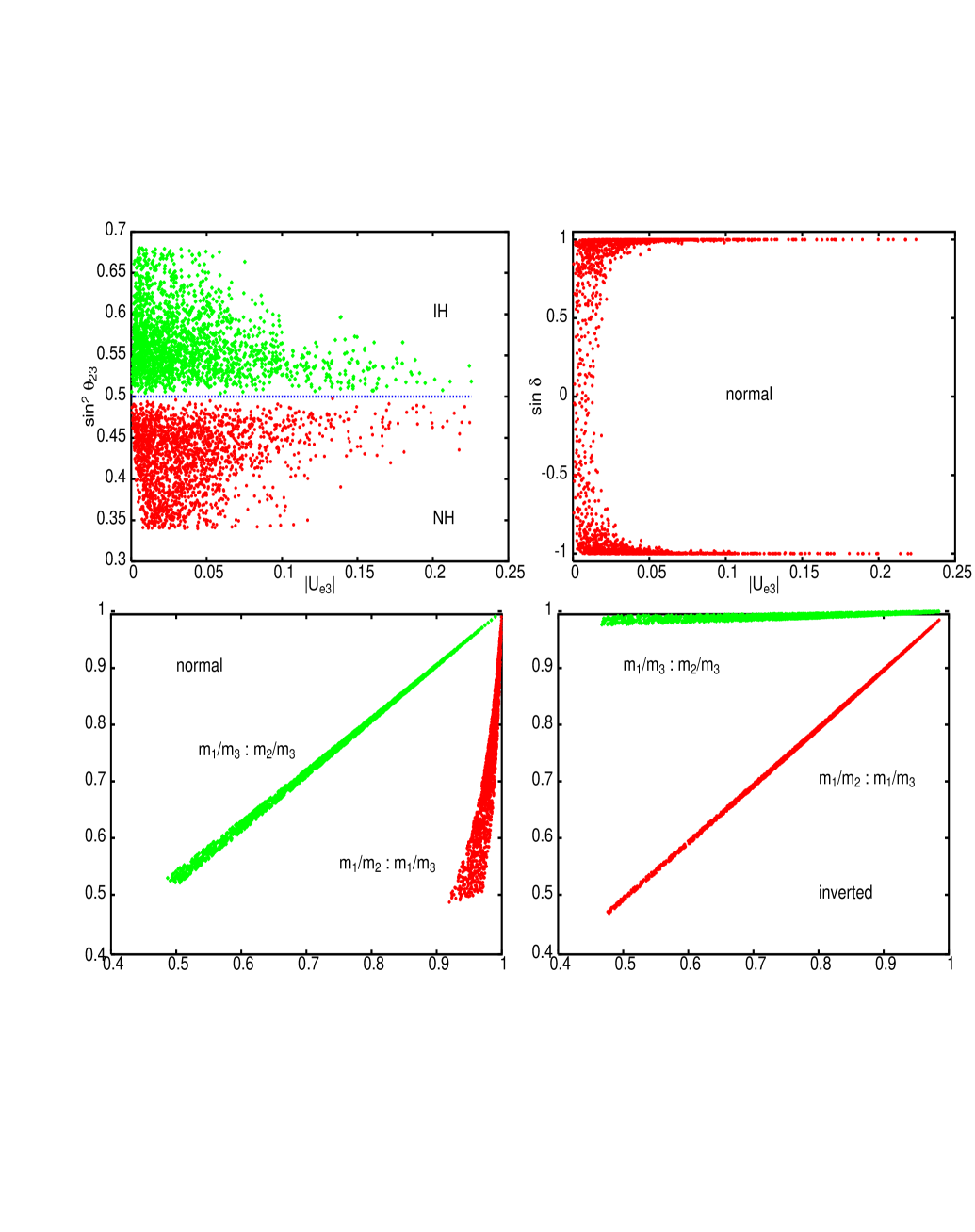We plot in Fig. 1 some of the correlations obtained for parameters around the values given above. The oscillation parameters are required to lie within the $3\sigma$ ranges from Ref. [27]. In fact, just demanding zero entries in the $e\mu$ and $\mu\mu$ elements will lead to such a behavior of the observables [26]. Indeed, as can be seen from the Figure, the neutrinos are close in mass, atmospheric neutrino mixing is not maximal and lies above (below) $\pi/4$ for the inverted (normal) mass ordering. Furthermore, $CP$ violation is basically maximal for sizable values of $|U_{e3}|$.

3 Renormalization Group Effects

As the flavor symmetry $L_{\mu}-L_{\tau}$ leads to quasi–degenerate neutrino masses, strong running of the mixing angles is generically expected [18, 20]. Typically, the running of the mixing angles $\theta_{ij}$ in a quasi–degenerate mass scheme with a common mass scale $m_{0}$ is proportional to $m_{0}^{2}/(m_{i}^{2}-m_{j}^{2})$ and therefore particularly strong for $\theta_{12}$. This behavior turns out to hold not only for the running between the scale of the lightest heavy Majorana neutrino and the weak scale, but also when the running between the see–saw scales is taken into account [21, 22]. The heavy Majorana neutrinos have to be integrated out one after the other, leading to a series of effective theories. It turns out that the running of the observables between the scales $M_{3}$ and $M_{2}$ or $M_{2}$ and $M_{1}$ can be of the same order as the running between $M_{1}$ and $M_{Z}$. In general this leads to quite involved expressions for the $\beta$–functions. However, in our case the structure of the Dirac and charged lepton mass matrices (i.e., the fact that they are diagonal) simplifies matters considerably and allows for some analytic understanding of the numerical results. All of the expressions we give in this Section are understood to be precise to order $|U_{e3}|$ and can be obtained with the help of Refs. [20, 22]. For instance, the $\beta$–functions for the mixing angles are:

$$16\pi^{2}\,\dot{\theta}_{12}\simeq \frac{m_{0}^{2}}{\mbox{$\Delta m^{2}_{\odot}$}}\left(1+\cos\left(\varphi_{2}-\varphi_{1}\right)\right)\,\sin 2\theta_{12}\,\left[P_{11}-\left(P_{22}\,\cos^{2}\theta_{23}+P_{33}\,\sin^{2}\theta_{23}\right)\right]~{},$$

$$32\pi^{2}\,\dot{\theta}_{13}\simeq \frac{m_{0}^{2}}{\mbox{$\Delta m^{2}_{\rm A}$}}\left(\cos\left(\delta-\varphi_{1}\right)-\cos\left(\delta-\varphi_{2}\right)\right)\,\sin 2\theta_{12}\,\sin 2\theta_{23}\,\left(P_{22}-P_{33}\right)~{},$$ (20)

$$16\pi^{2}\,\dot{\theta}_{23}\simeq \frac{m_{0}^{2}}{\mbox{$\Delta m^{2}_{\rm A}$}}\left[\left(1+\cos\varphi_{2}\right)\,\cos^{2}\theta_{12}+\left(1+\cos\varphi_{1}\right)\,\sin^{2}\theta_{12}\right]\,\sin 2\theta_{23}\,\left(P_{22}-P_{33}\right)~{}.$$

Note that since $\varphi_{1}\simeq\varphi_{2}$ there is no cancellation in the first relation for $\dot{\theta}_{12}$. The matrix $P$ in the above equations is given in the SM and in the Minimal Supersymmetric Standard Model (MSSM) by

$$P=\left\{\begin{array}[]{cl}-\frac{3}{2}Y_{e}Y_{e}^{\dagger}+\frac{1}{2}Y_{\nu}Y_{\nu}^{\dagger}&\mathrm{SM}~{},\\[5.69046pt] Y_{e}Y_{e}^{\dagger}+Y_{\nu}Y_{\nu}^{\dagger}&\mathrm{MSSM}~{}.\\ \end{array}\right.$$ (21)

Since in our model both $Y_{\nu}=m_{D}/v$ and $Y_{e}=m_{\ell}/v$ are diagonal, $P$ is diagonal as well and no off–diagonal elements appear in Eq. (3). With the values of the parameters in $m_{D}$ as given in Section 2 (i.e., $a\ll b\sim d={\cal O}(0.1)$) we can safely neglect $P_{11}$. This leads in particular to a negative $\beta$–function for $\theta_{12}$. Hence, this angle will become larger when evolved from high to low scales. Neglecting further the charged lepton Yukawas in $Y_{e}$ above the see–saw scales and noting that $P_{22}\simeq b^{2}/2$ and $P_{33}\simeq d^{2}/2$ for the SM and twice those values for the MSSM, we see that the running of $\theta_{13}$ and $\theta_{23}$ is suppressed with respect to the running of $\theta_{12}$ due to two reasons: firstly, it is inverse proportional to $\Delta m^{2}_{\rm A}$ and secondly, it is proportional to $P_{22}-P_{33}\propto b^{2}-d^{2}$, which is smaller than $P_{22}+P_{33}$, on which the running of $\theta_{12}$ (approximately) depends. Hence, the running of $\theta_{13}$ and $\theta_{23}$ is suppressed by $R~{}(b^{2}-d^{2})/b^{2}$ above the see–saw scales.

Below the see–saw scales only the tau–lepton Yukawa coupling $y_{\tau}$ governs the RG corrections. In this regime the evolution goes like [20]

$$16\,\pi^{2}\,\dot{\theta}_{12}\simeq-y_{\tau}^{2}\,\sin 2\theta_{12}\,\sin^{2}\theta_{23}\,\frac{m_{0}^{2}}{\mbox{$\Delta m^{2}_{\odot}$}}\left(1+\cos(\varphi_{2}-\varphi_{1})\right)~{},$$ (22)

in the MSSM, which is again negative and leads to sizable running. The formulae for the running of $\theta_{13,23}$ are again suppressed by roughly a factor $R$.

The phases stay almost constant in the whole range, because one can show that for our model $\dot{\varphi}_{1}$ and $\dot{\varphi}_{2}$ are mainly proportional to $\sin\varphi_{1}$ and $\sin\varphi_{2}$, respectively. Roughly the same behavior is found below $M_{1}$. Finally, the RG effects on the neutrino masses correspond predominantly to a rescaling, since the flavor–diagonal couplings, i.e., gauge couplings and the quartic Higgs coupling, dominate the evolution [19].

We can analyze if the zero entries in the mass matrix Eq. (16) remain zero entries. Below the see–saw scale it is well known that the RG corrections are multiplicative on the mass matrix, a fact which leaves zero entries zero. Taking the running in between the heavy Majorana masses into account, one can factorize the renormalization group effects $Z_{\mathrm{ext}}$ from the tree–level neutrino mass matrix in the MSSM as [23]

$$m_{\nu}=Z_{\mathrm{ext}}^{T}\,m_{\nu}^{0}\,Z_{\mathrm{ext}}\;.$$ (23)

Since in our model the neutrino and the charged lepton Yukawa coupling matrices are diagonal, the renormalization group effects are flavour diagonal, too. Therefore, texture zeroes in the charged lepton basis remain zero. With the already mentioned simplifications, $Z_{\mathrm{ext}}$ is approximately given by

$$16\pi^{2}\left(Z^{\mathrm{MSSM}}_{\mathrm{ext}}-\mathbbm{1}\right)=\mathrm{diag}\left(0,\,b^{2}\ln\frac{M\,Y}{\Lambda},\,d^{2}\ln\frac{M\,Y}{\Lambda}+y_{\tau}^{2}\ln\frac{v}{\Lambda}\right)\\ +b^{2}\ln\frac{M\,Y}{\Lambda}+d^{2}\ln\frac{M\,Y}{\Lambda}+\left[-\frac{3}{5}g_{1}^{2}-3g_{2}^{2}+3y_{t}^{2}\right]\ln\frac{v}{\Lambda}\;,$$ (24)

where $\left(g_{2},\,g_{1}\right)$ are the gauge couplings of the electroweak interactions $SU(2)_{L}\times U(1)_{Y}$, $y_{t}$ and $y_{\tau}$ are the top quark and $\tau$ Yukawa couplings, respectively and $\Lambda$ is the GUT scale of $2\cdot 10^{16}$ GeV.

In the extended SM, however, there are additional corrections which can not be factorized. They are responsible for the instability of texture zeroes under the renormalization group in the SM [22, 23]. We checked that for most observables the running behavior in the SM is similar to the running in case of the MSSM. The solar neutrino mixing angle receives however more RG corrections in the SM, a fact which can be traced back to the appearance of an $e\mu$ entry in the mass matrix Eq. (16). One might wonder at this point if this filling of zero entries would allow one to generate successful phenomenology from a mass matrix obeying the flavor symmetry $L_{\mu}-L_{\tau}$ without any breaking, i.e., just from Eq. (6). Recall, however, that in the SM $L_{\mu}-L_{\tau}$ is anomaly free and therefore the texture of the mass matrix is stable.

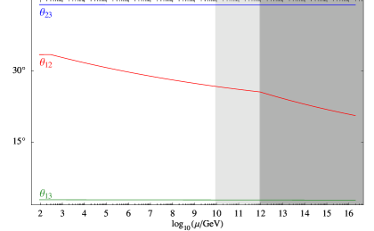
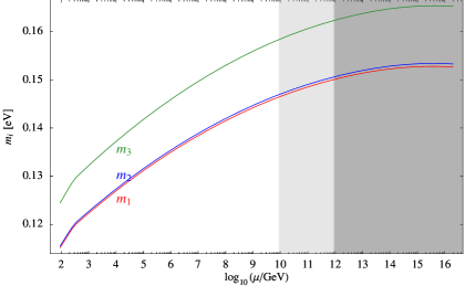
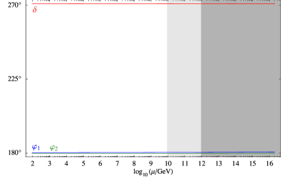
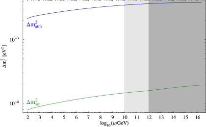
We plot in Fig. 2 the running of the angles, phases and masses for a typical example in the MSSM for $\tan\beta=10$ [28]. The resulting neutrino parameters at the GUT scale are $\sin^{2}\theta_{12}=0.123$, $U_{e3}=0.0484\,e^{i4.73}$, $\sin^{2}\theta_{23}=0.481$, $(m_{1},\,m_{2},\,m_{3})=(0.1527,\,0.1533,\,0.1653)\mbox{ eV}$ with $\mbox{$\Delta m^{2}_{\odot}$}=1.9\cdot 10^{-4}\mbox{ eV}^{2}$ and $\mbox{$\Delta m^{2}_{\rm A}$}=3.8\cdot 10^{-3}\mbox{ eV}^{2}$. They are changed by the renormalization group evolution to $\sin^{2}\theta_{12}=0.303$, $U_{e3}=0.0496\,e^{i4.73}$, $\sin^{2}\theta_{23}=0.481$, $(m_{1},\,m_{2},\,m_{3})=(0.1152,\,0.1155,\,0.1245)\mbox{ eV}$ with $\mbox{$\Delta m^{2}_{\odot}$}=7.9\cdot 10^{-5}\mbox{ eV}^{2}$ and $\mbox{$\Delta m^{2}_{\rm A}$}=2.1\cdot 10^{-3}\mbox{ eV}^{2}$. Note that the phases and $\theta_{13,23}$ remain practically constant, whereas $\sin^{2}\theta_{12}$ and $\Delta m^{2}_{\odot,\rm A}$ are changed by factors of up to three, and that the running in between and above the see–saw scales is at least as important as the running below them. This implies that radiative corrections, in particular for $\theta_{12}$ and the mass squared differences, can be crucial if one wishes to make meaningful phenomenological predictions of a given model.

$L^{\prime}$	matrix	comments
$\begin{array}[]{c}L_{e}\\ \mbox{\small normal hierarchy}\\ \mbox{\small always small RG effects}\end{array}$	$\left(\begin{array}[]{ccc}0&0&0\\ \cdot&a&b\\ \cdot&\cdot&d\end{array}\right)$	$\begin{array}[]{c}R=\frac{\mbox{$\Delta m^{2}_{\odot}$}}{\mbox{$\Delta m^{2}_{\rm A}$}}\simeq|U_{e3}|^{2}\\ \tan^{2}\theta_{\rm atm}\simeq 1+|U_{e3}|\simeq 1+\sqrt{R}\\ {\mbox{$\langle m\rangle$}\simeq\sqrt{\mbox{$\Delta m^{2}_{\rm A}$}}\,|U_{e3}|^{2}\simeq\sqrt{\mbox{$\Delta m^{2}_{\odot}$}}}\end{array}$
$\begin{array}[]{c}L_{e}-L_{\mu}-L_{\tau}\\ \mbox{\small inverted hierarchy}\\ \mbox{\small small RG effects (pseudo--Dirac)}\end{array}$	$\left(\begin{array}[]{ccc}0&a&b\\ \cdot&0&0\\ \cdot&\cdot&0\end{array}\right)$	$\begin{array}[]{c}\mbox{requires }U_{\ell}\mbox{: ideal for QLC}\\ \mbox{$\tan^{2}\theta_{\rm\odot}$}\simeq 1-4\,|U_{e3}|\stackrel{{\scriptstyle?}}{{\simeq}}1-2\sqrt{2}\,{\sin\theta_{\rm C}}\\ {\mbox{$\langle m\rangle$}\simeq\sqrt{\mbox{$\Delta m^{2}_{\rm A}$}}}\end{array}$
$\begin{array}[]{c}{L_{\mu}-L_{\tau}}\\ \mbox{\small quasi--degeneracy}\\ \mbox{\small always large RG effects}\end{array}$	$\left(\begin{array}[]{ccc}a&0&0\\ \cdot&0&b\\ \cdot&\cdot&0\end{array}\right)$	$\begin{array}[]{c}\mbox{in leading order:}\\ U_{e3}=0\mbox{ and }\theta_{23}=\pi/4\\ {\mbox{$\langle m\rangle$}\simeq m_{0}}\end{array}$

Table 2: The three simple $U(1)$ charges as implied by current data, the zeroth order mass matrix and some comments on their phenomenology.

4 Conclusions and Summary

Identifying the structure of the mass matrix $m_{\nu}$ is one of the main goals of neutrino physics. Current data seems to point towards three interesting forms of $m_{\nu}$, each corresponding to the (approximative) conservation of a non–standard lepton charge. While $L_{e}$ and $L_{e}-L_{\mu}-L_{\tau}$ are well known cases — leading to the normal and inverted hierarchy, respectively — the third possibility $L_{\mu}-L_{\tau}$ has not been examined in as much detail. Since quasi–degenerate neutrinos are predicted by the conservation of $L_{\mu}-L_{\tau}$, this case is easily testable. Moreover, since the mass matrix is automatically $\mu$–$\tau$ symmetric, further phenomenological support is provided. We stress again that the three possibilities $L_{e}$, $L_{e}-L_{\mu}-L_{\tau}$ and $L_{\mu}-L_{\tau}$ differ in particular by their prediction for neutrinoless double beta decay, a fact which will easily allow to identify the correct one. In Table 2 the relevant matrices and some aspects of their phenomenology are summarized. Here we analyzed the consequences of a see–saw model based on $L_{\mu}-L_{\tau}$, which predicts, e.g., non–maximal atmospheric neutrino mixing, large $CP$ violation and quasi–degenerate neutrinos. This last aspect makes radiative corrections be particularly important and we carefully analyzed their effects both numerically and analytically. We showed explicitely that running between the see–saw scales is at least as important as running from the lowest see–saw scale down to low energies.

Acknowledgments

We thank R. Foot for discussions and W.R. wishes to thank S. Choubey for a fruitful collaboration. This work was supported by the “Deutsche Forschungsgemeinschaft” in the “Sonderforschungsbereich 375 für Astroteilchenphysik” and under project number RO–2516/3–1.

Figure 1: Scatter plots of some of the observables resulting from a mass matrix with zero $e\mu$ and $\mu\mu$ elements. We required the $3\sigma$ values for the oscillation parameters from [27].

Figure 2: Typical plot for the evolution of the mixing angles and masses from the GUT scale $2\times 10^{16}$ GeV to low scale. In this example, we have $\tan\beta=10$ and the parameters in the matrix Eq. (16) at the GUT scale are $a=0.0066926$, $b=0.0692883$, $c=0.0697464$, $X=0.0096528$, $Y=1$, $\epsilon_{1}=0.0005595$, $\epsilon_{2}=0.0749098$, $\varphi=2.45376$ and $M=9.098937108\cdot 10^{11}$ GeV.

References

- [1] For an overview of the current situation see, for instance: R. N. Mohapatra et al., hep-ph/0412099; S. T. Petcov, Talk given at the 21st International Conference on Neutrino Physics and Astrophysics (Neutrino 2004), June 14 – 19, 2004, Paris, France, Nucl. Phys. Proc. Suppl. 143, 159 (2005); hep-ph/0412410.
- [2] B. Pontecorvo, Zh. Eksp. Teor. Fiz. 33, 549 (1957) and 34, 247 (1958); Z. Maki, M. Nakagawa and S. Sakata, Prog. Theor. Phys. 28, 870 (1962).
- [3] P. Minkowski, Phys. Lett. B67, 421 (1977); T. Yanagida, in Proceedings of the Workshop on Unified Theory and the Baryon Number of the Universe, edited by O. Sawada and A. Sugamoto (KEK, Tsukuba, 1979), p. 95; M. Gell-Mann, P. Ramond, and R. Slansky, in Supergravity, edited by F. van Nieuwenhuizen and D. Freedman (North Holland, Amsterdam, 1979), p. 315; S.L. Glashow, in Quarks and Leptons, edited by M. L et al. (Plenum, New York, 1980), p. 707; R.N. Mohapatra and G. Senjanovic, Phys. Rev. Lett. 44, 912 (1980).
- [4] For recent overviews about the predictions for neutrinoless double beta decay, see S. Pascoli, S. T. Petcov and T. Schwetz, hep-ph/0505226; S. Choubey and W. Rodejohann, hep-ph/0506102.
- [5] W. Buchmuller and T. Yanagida, Phys. Lett. B 445, 399 (1999); F. Vissani, JHEP 9811, 025 (1998); see also the second paper in [6].
- [6] S. T. Petcov, Phys. Lett. B 110, 245 (1982); an incomplete list of more recent studies is: R. Barbieri et al., JHEP 9812, 017 (1998); A. S. Joshipura and S. D. Rindani, Eur. Phys. J. C 14, 85 (2000); R. N. Mohapatra, A. Perez-Lorenzana and C. A. de Sousa Pires, Phys. Lett. B 474, 355 (2000); Q. Shafi and Z. Tavartkiladze, Phys. Lett. B 482, 145 (2000). L. Lavoura, Phys. Rev. D 62, 093011 (2000); T. Kitabayashi and M. Yasue, Phys. Rev. D 63, 095002 (2001); K. S. Babu and R. N. Mohapatra, Phys. Lett. B 532, 77 (2002); H. J. He, D. A. Dicus and J. N. Ng, Phys. Lett. B 536, 83 (2002) H. S. Goh, R. N. Mohapatra and S. P. Ng, Phys. Lett. B 542, 116 (2002); G. K. Leontaris, J. Rizos and A. Psallidas, Phys. Lett. B 597, 182 (2004); W. Grimus and L. Lavoura, J. Phys. G 31, 683 (2005).
- [7] P. H. Frampton, S. T. Petcov and W. Rodejohann, Nucl. Phys. B 687, 31 (2004); S. T. Petcov and W. Rodejohann, Phys. Rev. D 71, 073002 (2005).
- [8] W. Rodejohann, Phys. Rev. D 69, 033005 (2004).
- [9] M. Raidal, Phys. Rev. Lett. 93, 161801 (2004); H. Minakata and A. Y. Smirnov, Phys. Rev. D 70, 073009 (2004); for a review and more references, see H. Minakata, hep-ph/0505262.
- [10] P. Binetruy et al., Nucl. Phys. B 496, 3 (1997); N. F. Bell and R. R. Volkas, Phys. Rev. D 63, 013006 (2001).
- [11] K. S. Babu, E. Ma and J. W. F. Valle, Phys. Lett. B 552, 207 (2003); M. Hirsch et al., Phys. Rev. D 69, 093006 (2004).
- [12] S. Choubey and W. Rodejohann, Eur. Phys. J. C 40, 259 (2005).
- [13] N. Arkani-Hamed et al., Phys. Rev. D 64, 115011 (2001); F. Borzumati and Y. Nomura, Phys. Rev. D 64, 053005 (2001); R. Kitano, Phys. Lett. B 539, 102 (2002); R. Arnowitt, B. Dutta and B. Hu, Nucl. Phys. B 682, 347 (2004); S. Abel, A. Dedes and K. Tamvakis, Phys. Rev. D 71, 033003 (2005); C. Hagedorn and W. Rodejohann, JHEP 0507, 034 (2005); S. Antusch, O. J. Eyton-Williams and S. F. King, hep-ph/0505140.
- [14] C. S. Lam, Phys. Lett. B 507, 214 (2001); K. R. S. Balaji, W. Grimus and T. Schwetz, Phys. Lett. B 508, 301 (2001); W. Grimus and L. Lavoura, JHEP 0107, 045 (2001); Eur. Phys. J. C 28, 123 (2003); E. Ma, Phys. Rev. D 66, 117301 (2002); T. Kitabayashi and M. Yasue, Phys. Rev. D 67, 015006 (2003); P. F. Harrison and W. G. Scott, Phys. Lett. B 547, 219 (2002); Y. Koide, Phys. Rev. D 69, 093001 (2004); W. Grimus et al., Nucl. Phys. B 713, 151 (2005); R. N. Mohapatra, JHEP 0410, 027 (2004); R. N. Mohapatra, S. Nasri and H. B. Yu, hep-ph/0502026; C. S. Lam, hep-ph/0503159; I. Aizawa, T. Kitabayashi and M. Yasue, hep-ph/0504172; K. Matsuda and H. Nishiura, hep-ph/0506192.
- [15] X. G. He et al., Phys. Rev. D 43, 22 (1991); Phys. Rev. D 44, 2118 (1991); see also E. Ma, D. P. Roy and S. Roy, Phys. Lett. B 525, 101 (2002).
- [16] R. Foot, hep-ph/0505154.
- [17] K. S. Babu, C. N. Leung and J. T. Pantaleone, Phys. Lett. B 319, 191 (1993); S. Antusch et al., Phys. Lett. B 519, 238 (2001).
- [18] M. Tanimoto, Phys. Lett. B 360, 41 (1995); J. R. Ellis and S. Lola, Phys. Lett. B 458, 310 (1999). P. H. Chankowski, W. Krolikowski and S. Pokorski, Phys. Lett. B 473, 109 (2000); J. A. Casas et al., Nucl. Phys. B 573, 652 (2000); N. Haba, Y. Matsui and N. Okamura, Eur. Phys. J. C 17, 513 (2000); K. R. S. Balaji et al., Phys. Rev. D 63, 113002 (2001); M. Frigerio and A. Y. Smirnov, JHEP 0302, 004 (2003).
- [19] P. H. Chankowski and S. Pokorski, Int. J. Mod. Phys. A 17, 575 (2002).
- [20] S. Antusch et al., Nucl. Phys. B 674, 401 (2003).
- [21] S. F. King and N. N. Singh, Nucl. Phys. B591 3, (2000); S. Antusch et al., Phys. Lett. B538 87, (2002); B. Stech and Z. Tavartkiladze, Phys. Rev. D70 035002, (2004); J. W. Mei, Phys. Rev. D 71, 073012 (2005); J. Ellis et al., hep-ph/0506122.
- [22] S. Antusch et al., JHEP 0503, 024 (2005).
- [23] M. Lindner, M. A. Schmidt and A. Y. Smirnov, hep-ph/0505067.
- [24] G. C. Branco et al., Phys. Rev. D 67, 073025 (2003).
- [25] P. H. Frampton, S. L. Glashow and D. Marfatia, Phys. Lett. B 536, 79 (2002); Z. Z. Xing, Phys. Lett. B 539, 85 (2002) B. R. Desai, D. P. Roy and A. R. Vaucher, Mod. Phys. Lett. A 18, 1355 (2003); W. L. Guo and Z. Z. Xing, Phys. Rev. D 67, 053002 (2003).
- [26] Z. Z. Xing, Phys. Lett. B 530, 159 (2002).
- [27] M. Maltoni et al., New J. Phys. 6, 122 (2004); hep-ph/0405172v4.
- [28] Such figures can be obtained with the software package REAP introduced in [22] and available at http://www1.physik.tu-muenchen.de/rge/.