B-Meson Wavefunction with Contributions from 3-particle Fock States

Abstract

The B-meson light-cone wavefunctions, $\Psi_{\pm}(\omega,z^{2})$, are investigated up to the next-to-leading order in Fock state expansion in the heavy quark limit. In order to know the transverse momentum dependence of the B-meson wavefunctions with 3-particle Fock states’ contributions, we make use of the relations between 2- and 3- particle wavefunctions derived from the QCD equations of motion and the heavy quark symmetry, especially two constraints derived from the gauge field equation of motion are employed. Our results show that the use of gluon equation of motion can give a constraint on the transverse momentum dependence $\chi(\omega,\mathbf{k}_{\perp})$ of the B-meson wavefunctions, whose distribution tends to be a hyperbola-like curve under the condition $0<c_{1}<1$, which is quite different from the WW type wavefunctions, whose transverse momentum dependence $\chi^{WW}(\omega,\mathbf{k}_{\perp})$ is merely a delta function. Based on the derived results, we propose a simple model for the B-meson wavefunctions with 3-particle Fock states’ contributions.

PACS numbers: 12.38.Aw, 12.39.Hg, 14.40.Nd

Keywords: B-meson wavefunction, 3-particle Fock state, heavy quark symmetry

I Introduction

The non-perturbative light-cone (LC) wavefunction (WF)/distribtuion amplitude (DA) of the B meson plays an important role for making reliable predictions for exclusive B meson decays. The B-meson DA has been investigated in various approaches bdistribution1 ; bdistribution2 ; braun ; lange ; qiao0 ; beneke ; descotes ; geyer ; alex . Recently, Ref.libwave claims that it is the B-meson WF rather than the B-meson DA that is more relevant to the B decays, and in the framework of the $k_{T}$-factorization theorem kt , they proved that the B-meson WF is renormalizable after taking into account the renormalization-group (RG) evolution effects, meanwhile, the undesirable feature braun of the B-meson DA under evolution can be removed. Since the B-meson WF still poses a major source of uncertainty in the study of the B decays, hence, theoretically, it is an important issue to study on it.

Ref. qiao , as well bwave , presents an analytic solution for the B-meson WFs $\Psi_{\pm}(\omega,z^{2})$, which satisfies the constraints from the QCD equations of motion and the heavy-quark symmetry heavyquark . It is found that in the Wandzura-Wilczek(WW) approximation ww , which corresponds to the valence quark distribution, the B-meson WFs can be determined uniquely in terms of the “effective mass”, the $\bar{\Lambda}$, defined in the Heavy Quark Effective Theory (HQET) hqet . Ref.huangwu shows that when taking $\bar{\Lambda}\in(0.5GeV,0.6GeV)$, one can give a reasonable perturbative QCD result for $B\to\pi$ transition form factor that is consistent with what was obtained in the LC sum rule calculation sumrule and the lattice QCD simulation lattice .

It should be noted that in the WW approximation, the obtained analytic results for the B-meson WFs $\Psi_{\pm}(\omega,z^{2})$ are unique, and the only missing part for practical numerical use is the RG evolution effect. However, there is very limited knowledge on the higher Fock states’ contributions. In Ref.qiao0 , the B-meson distributions $\phi_{\pm}(\omega)$ with 3-particle Fock states are given and a rough estimation presented there shows that the 3-particle Fock states’ contributions might considerably broaden the transverse momentum distribution that is derived from the WW approximation. Recently, based on the QCD sum rule analysis and taking only the two 3-particle distributions $\Psi_{A}(\rho,\xi)$ and $\Psi_{V}(\rho,\xi)$ into consideration, Ref.alex connects the asymptotic behavior of their difference to the well-known quark-antiquark-gluon DA $\varphi_{3\pi}(\alpha_{i})$ ($\alpha_{i}(i=1,2,3)$ are the fractions of the pion momentum carried by the corresponding partons and satisfy $\alpha_{1}+\alpha_{2}+\alpha_{3}=1$), i.e. in the small $\rho$ and $\xi$ region, $\Psi_{V}(\rho,\xi)-\Psi_{A}(\rho,\xi)\sim\varphi_{3\pi}(\alpha_{1},1-\alpha_{1}-\alpha_{3},\alpha_{3})|_{\alpha_{1}=\rho/m_{B},\alpha_{3}=\xi/m_{B}}\sim\rho\xi^{2}$.

In this paper, we are going to investigate the B-meson WFs $\Psi_{\pm}(\omega,z^{2})$ with the contributions from 3-particle Fock states. From the heavy-quark symmetry and the equations of motion for the light degrees of freedom, we get several constraints on the behaviors of WFs. By adopting some assumptions, we will solve the B-meson WFs approximately, especially, by taking the aforementioned asymptotic behavior of the difference between $\Psi_{A}(\rho,\xi)$ and $\Psi_{V}(\rho,\xi)$ into account, we try to derive an explicit form for the B-meson distributions $\phi_{\pm}(\omega)$ that include the 3-particle Fock states’ contributions.

The paper is organized as follows. In Sec.II, several differential equations for the B-meson WFs are obtained by using the heavy quark symmetry and the equations of motion for the light degrees of freedom. In Sec.III, approximate solutions for the B-meson WFs including the contributions from the 3-particle Fock states are investigated under three assumptions. A new model for the B-meson WFs and some discussions over its phenomenological implication are presented in Sec.IV. The last section is reserved for a summary.

II Differential equations for the B-meson wavefunctions

In HQET, the B-meson WFs $\tilde{\Psi}_{\pm}(t,z^{2})$ can be defined in terms of the vacuum-to-meson matrix element of the nonlocal operators grozin :

$$\langle 0|\bar{q}(z)\Gamma h_{v}(0)|\bar{B}(p)\rangle=-\frac{if_{B}M}{2}{\rm Tr}\Bigg{[}\gamma_{5}\Gamma\frac{1+/\!\!\!v}{2}\!\!\!\times\Bigg{\{}\tilde{\Psi}_{+}(t,z^{2})-/\!\!\!z\frac{\tilde{\Psi}_{+}(t,z^{2})-\tilde{\Psi}_{-}(t,z^{2})}{2t}\Bigg{\}}\Bigg{]},$$ (1)

where $z^{\mu}=(0,z^{-},\mathbf{z}_{\perp})$, $z^{2}=-\mathbf{z}_{\perp}^{2}$, $v^{2}=1$, $t=v\cdot z$, and $p^{\mu}=Mv^{\mu}$ is the 4-momentum of the B meson with mass $M$, $h_{v}(x)$ denotes the effective $b$-quark field and $\Gamma$ is a generic Dirac matrix. The path-ordered gauge factors are implied between the constituent fields. Note that in the above definition, the separation between quark and antiquark is not restricted on the LC ($z^{2}=0$). For a fast moving meson, $t\to\infty$, Eq.(1) shows that $\tilde{\Psi}_{+}(t,z^{2})$ is the leading-twist WF and $\tilde{\Psi}_{-}(t,z^{2})$ is the subleading one. To know more about the twist structures for the B meson, readers are recommended to refer to Ref.geyer for details, where the relation between the geometric twist and the dynamic twist was discussed.

In the heavy quark limit, the general Lorentz decomposition of the 3-particle matrix elements can attribute to four independent 3-particle WFs similar to the 3-particle LC DAs qiao , i.e. $\tilde{\Psi}_{V}(t,u,z^{2})$, $\tilde{\Psi}_{A}(t,u,z^{2})$, $\tilde{X}_{A}(t,u,z^{2})$ and $\tilde{Y}_{A}(t,u,z^{2})$:

$$\langle 0|\bar{q}(z)\,gG_{\mu\nu}(uz)\,z^{\nu}\,\Gamma\,h_{v}(0)|\bar{B}(p)\rangle$$

$$= \frac{1}{2}\,f_{B}M\,{\rm Tr}\,\left[\,\gamma_{5}\,\Gamma\,\frac{1+\not{\!v}}{2}\,\biggl{\{}(v_{\mu}\not{\!z}-t\,\gamma_{\mu})\ \left(\tilde{\Psi}_{A}(t,u,z^{2})-\tilde{\Psi}_{V}(t,u,z^{2})\right)\right.$$

$$-i\,\sigma_{\mu\nu}z^{\nu}\,\tilde{\Psi}_{V}(t,u,z^{2})-\left.\left(z_{\mu}-\frac{z^{2}v_{\mu}}{t}\right)\tilde{X}_{A}(t,u,z^{2})\,+\left(\frac{z_{\mu}}{t}\not{\!z}-\frac{z^{2}\gamma_{\mu}}{t}\right)\,\tilde{Y}_{A}\,(t,u,z^{2})\biggr{\}}\,\right]\ .$$

Here, the $z^{2}$-dependent terms are kept explicitly in order to get the transverse momentum dependence of the B-meson WFs.

By using the equation of motion for the light quark, $\bar{q}\stackrel{{\scriptstyle\leftarrow}}{{\not{\!\!D}}}=0$, and HQET equation of motion for the heavy quark, $v\cdot Dh_{v}=0$, one can obtain four independent differential equations, which correlate $\tilde{\Psi}_{+}(t,z^{2})$ and $\tilde{\Psi}_{-}(t,z^{2})$ to the 3-particle WFs:

$$\frac{\partial\tilde{\Psi}_{-}(t,z^{2})}{\partial t} - \frac{\tilde{\Psi}_{+}(t,z^{2})-\tilde{\Psi}_{-}(t,z^{2})}{t}-\frac{z^{2}}{t}\frac{\partial}{\partial z^{2}}[\tilde{\Psi}_{+}(t,z^{2})-\tilde{\Psi}_{-}(t,z^{2})]$$ (3)

$$= \int_{0}^{1}udu\;\left[2t[\tilde{\Psi}_{A}(t,u,z^{2})-\tilde{\Psi}_{V}(t,u,z^{2})]+3\frac{z^{2}}{t}\tilde{Y}_{A}(t,u,z^{2})-\frac{z^{2}}{t}\tilde{X}_{A}(t,u,z^{2})\right],$$

$$\frac{\partial\tilde{\Psi}_{+}(t,z^{2})}{\partial t} - \frac{\partial\tilde{\Psi}_{-}(t,z^{2})}{\partial t}-\frac{\tilde{\Psi}_{+}(t,z^{2})-\tilde{\Psi}_{-}(t,z^{2})}{t}+4t\frac{\partial\tilde{\Psi}_{+}(\omega,z^{2})}{\partial z^{2}}$$ (4)

$$= \int_{0}^{1}udu\;2t[\tilde{\Psi}_{A}(t,u,z^{2})+2\,\tilde{\Psi}_{V}(t,u,z^{2})+\tilde{X}_{A}(t,u,z^{2})],$$

$$\frac{\partial\tilde{\Psi}_{+}(t,z^{2})}{\partial t} - \frac{1}{2t}\left[\tilde{\Psi}_{+}(t,z^{2})-\tilde{\Psi}_{-}(t,z^{2})\right]+i\bar{\Lambda}\tilde{\Psi}_{+}(t,z^{2})+2t\frac{\partial\tilde{\Psi}_{+}(t,z^{2})}{\partial z^{2}}$$ (5)

$$\!\!\!\!\!\!\!\!\!\!\!\!\!\!\!\!\!\!=\int_{0}^{1}du\,(u-1)\,\left[t[\tilde{\Psi}_{A}(t,u,z^{2})+\tilde{X}_{A}(t,u,z^{2})]-\frac{z^{2}}{t}\tilde{X}_{A}(t,u,z^{2})+\frac{z^{2}}{t}\tilde{Y}_{A}(t,u,z^{2})\right]$$

and

$$\frac{\tilde{\Psi}_{+}(t,z^{2})}{\partial t} - \frac{\tilde{\Psi}_{-}(t,z^{2})}{\partial t}+\left(i\bar{\Lambda}-\frac{1}{t}\right)\left[\tilde{\Psi}_{+}(t,z^{2})-\tilde{\Psi}_{-}(t,z^{2})\right]+2t\left[\frac{\partial\tilde{\Psi}_{+}(t,z^{2})}{\partial z^{2}}-\frac{\partial\tilde{\Psi}_{-}(t)}{\partial z^{2}}\right]$$ (6)

$$= 2t\,\int_{0}^{1}du\,(u-1)\,[\tilde{\Psi}_{A}(t,u,z^{2})+\tilde{Y}_{A}(t,u,z^{2})]\ ,$$

where $\bar{\Lambda}=M-m_{b}=\frac{iv\cdot\partial\langle 0|\bar{q}\Gamma h_{v}|\bar{B}(p)\rangle}{\langle 0|\bar{q}\Gamma h_{v}|\bar{B}(p)\rangle}$ is the usual “effective mass” of the B meson in the HQET. By taking the LC limit, one may easily find that our present results agree with those in Ref.qiao . Making the Fourier transformation, by virtue of the formulae given in the appendix, we obtain,

$$\omega\frac{\partial\Psi_{-}(\omega,z^{2})}{\partial\omega}+z^{2}\left[\frac{\partial\Psi_{+}(\omega,z^{2})}{\partial z^{2}}-\frac{\partial\Psi_{-}(\omega,z^{2})}{\partial z^{2}}\right]+\Psi_{+}(\omega,z^{2}) = I(\omega,z^{2}),$$ (7)

$$\left[\omega\frac{\partial}{\partial\omega}+2\right](\Psi_{+}(\omega,z^{2})-\Psi_{-}(\omega,z^{2}))+4\frac{\partial^{2}}{\partial\omega^{2}}\frac{\partial\Psi_{+}(\omega,z^{2})}{\partial z^{2}} = J(\omega,z^{2})\;,$$ (8)

$$\left[(\omega-\bar{\Lambda})\frac{\partial}{\partial\omega}+\frac{3}{2}\right]\Psi_{+}(\omega,z^{2})-\frac{1}{2}\Psi_{-}(\omega,z^{2})+2\frac{\partial^{2}}{\partial\omega^{2}}\frac{\partial\Psi_{+}(\omega,z^{2})}{\partial z^{2}} = M(\omega,z^{2})+N(\omega,z^{2})$$ (9)

and

$$\bar{\Lambda}[\Psi_{+}(\omega,z^{2})-\Psi_{-}(\omega,z^{2})]+2\frac{\partial^{2}}{\partial\omega\partial z^{2}}[\Psi_{+}(\omega,z^{2})+\Psi_{-}(\omega,z^{2})] = L(\omega,z^{2})\;,$$ (10)

where the 3-particle source terms are

$$I(\omega,z^{2}) = 2\frac{d}{d\omega}\int_{0}^{\omega}d\rho\int_{\omega-\rho}^{\infty}\frac{d\xi}{\xi}\frac{\partial}{\partial\xi}\left[\Psi_{A}(\rho,\xi,z^{2})-\Psi_{V}(\rho,\xi,z^{2})\right]$$ (11)

$$-z^{2}\int_{0}^{\omega}d\rho\int_{\omega-\rho}^{\infty}\frac{d\xi}{\xi}\left(\frac{\omega-\rho}{\xi}\right)[X_{A}(\rho,\xi,z^{2})-3Y_{A}(\rho,\xi,z^{2})]\ ,$$

$$J(\omega,z^{2}) = 2\frac{d}{d\omega}\int_{0}^{\omega}d\rho\int_{\omega-\rho}^{\infty}\frac{d\xi}{\xi}\frac{\partial}{\partial\xi}\left[\Psi_{A}(\rho,\xi,z^{2})+2\Psi_{V}(\rho,\xi,z^{2})+X_{A}(\rho,\xi,z^{2})\right]\ ,$$ (12)

$$L(\omega,z^{2}) = -2\int_{0}^{\omega}d\rho\int_{\omega-\rho}^{\infty}\frac{d\xi}{\xi}\frac{\partial}{\partial\xi}[Y_{A}(\rho,\xi,z^{2})-2\Psi_{V}(\rho,\xi,z^{2})-X_{A}(\rho,\xi,z^{2})]$$ (13)

$$+2\frac{d}{d\omega}\int_{0}^{\omega}d\rho\int_{\omega-\rho}^{\infty}\frac{d\xi}{\xi}[\Psi_{A}(\rho,\xi,z^{2})+Y_{A}(\rho,\xi,z^{2})]\ ,$$

$$M(\omega,z^{2}) = \frac{d}{d\omega}\int_{0}^{\omega}d\rho\int_{\omega-\rho}^{\infty}\frac{d\xi}{\xi}\frac{\partial}{\partial\xi}\left[\Psi_{A}(\rho,\xi,z^{2})+X_{A}(\rho,\xi,z^{2})\right]$$ (14)

$$-\frac{d^{2}}{d\omega^{2}}\int_{0}^{\omega}d\rho\int_{\omega-\rho}^{\infty}\frac{d\xi}{\xi}[\Psi_{A}(\rho,\xi,z^{2})+X_{A}(\rho,\xi,z^{2})]$$

and

$$N(\omega,z^{2}) = z^{2}\int_{0}^{\omega}d\rho\int_{\omega-\rho}^{\infty}\frac{d\xi}{\xi}\left(\frac{\omega-\rho}{\xi}\right)[Y_{A}(\rho,\xi,z^{2})-X_{A}(\rho,\xi,z^{2})]$$ (15)

$$-z^{2}\int_{0}^{\omega}d\rho\int_{\omega-\rho}^{\infty}\frac{d\xi}{\xi}[Y_{A}(\rho,\xi,z^{2})-X_{A}(\rho,\xi,z^{2})]\ .$$

Secondly, by using Eq.(II) and the gluon equation of motion, $D^{\mu}G^{a}_{\mu\nu}(z)=0$, whose source term that induces even higher Fock state’ contribution is neglected in this work, one can obtain two more independent relations among the 3-particle WFs:

$$\left[3\tilde{\Psi}_{A}(t,u,z^{2})+4\tilde{Y}_{A}(t,u,z^{2})-\tilde{X}_{A}(t,u,z^{2})\right]+t\frac{\partial}{\partial t}\left[\tilde{\Psi}_{A}(t,u,z^{2})+2\tilde{Y}_{A}(t,u,z^{2})-\right.$$

$$\left.\tilde{X}_{A}(t,u,z^{2})\right]+z^{2}\left[\frac{1}{t^{2}}\left[\tilde{Y}_{A}(t,u,z^{2})-\tilde{X}_{A}(t,u,z^{2})\right]-\frac{1}{t}\frac{\partial}{\partial t}\left[\tilde{Y}_{A}(t,u,z^{2})-\tilde{X}_{A}(t,u,z^{2})\right]\right.$$

$$+2\frac{\partial}{\partial z^{2}}[\tilde{\Psi}_{A}(t,u,z^{2})\left.+\tilde{Y}_{A}(t,u,z^{2})]\right]=0$$ (16)

and

$$\frac{2}{t}[\tilde{X}_{A}(t,u,z^{2})-\tilde{Y}_{A}(t,u,z^{2})]+2\frac{z^{2}}{t}\frac{\partial}{\partial z^{2}}[\tilde{X}_{A}(t,u,z^{2})-\tilde{Y}_{A}(t,u,z^{2})]$$

$$-2t\frac{\partial}{\partial z^{2}}\left[\tilde{\Psi}_{A}(t,u,z^{2})+\tilde{X}_{A}(t,u,z^{2})\right]-\frac{\partial}{\partial t}\left[\tilde{\Psi}_{A}(t,u,z^{2})+\tilde{Y}_{A}(t,u,z^{2})\right]=0\ .$$ (17)

Taking the LC limit in Eq.(II), we get

$$\left[3\tilde{\Psi}_{A}(t,u)+4\tilde{Y}_{A}(t,u)-\tilde{X}_{A}(t,u)\right]+t\frac{\partial}{\partial t}\left[\tilde{\Psi}_{A}(t,u)+2\tilde{Y}_{A}(t,u)-\tilde{X}_{A}(t,u)\right]=0\ ,$$ (18)

with $F(t,u)=F(t,u,z^{2})|_{z^{2}\to 0}$ ($F=\{\tilde{\Psi}_{V},\tilde{\Psi}_{A},\tilde{X}_{A}\}$). By doing the Fourier transformation and exploiting the boundary conditions, $F(\rho,\xi)|_{\rho\to\infty,\xi\to\infty}\to 0$ (F=$\Psi_{A}$, $X_{A}$, $Y_{A}$), we obtain a relation among the double moments of the 3-particle DAs,

$$3\left[\Psi_{A}(\rho,\xi)\right]_{1}^{1}+4\left[Y_{A}(\rho,\xi)\right]_{1}^{1}=\left[X_{A}(\rho,\xi)\right]_{1}^{1},$$ (19)

where $\left[F\right]^{i}_{j}$ are double moments of the 3-particle distributions,

$$\left[F\right]^{i}_{j}=\int_{0}^{\infty}d\rho\int_{0}^{\infty}d\xi\ \rho^{i-j}\xi^{j-1}F(\rho,\xi)\ ,\qquad\left(F=\{\Psi_{V},\Psi_{A},X_{A}\}\right).$$

III Approximate solution for the B-meson WFs with 3-particle Fock states

In the following, we shall give an approximate solution for the B-meson WFs with 3-particle Fock states’ contributions by solving the differential equations as shown in Sec.II. Before doing this, as a basis and to be self-consistent, we first recollect the results in the WW approximation (i.e. $I(\omega)=J(\omega)=L(\omega)=M(\omega)=N(\omega)=0$), then, derive several constraints for the B-meson DAs $\phi_{\pm}(\omega)$, where the B-meson DAs can be obtained by taking the LC limit of the B-meson WFs, i.e. $\phi_{\pm}(\omega)\equiv\lim_{z^{2}\to 0}\Psi_{\pm}(\omega,z^{2})$.

III.1 B-meson WFs $\Psi^{WW}_{\pm}(\omega,z^{2})$ in the WW approximation

When ignoring the 3-particle Fock states’ contributions, i.e. setting $I(\omega)=J(\omega)=L(\omega)=M(\omega)=N(\omega)=0$, one can readily obtain the B-meson WW-type WFs $\Psi^{WW}_{\pm}(\omega,z^{2})$. In this case, the two DAs $\phi^{WW}_{\pm}(\omega)$ take the formbwave ; qiao0 :

$$\phi^{WW}_{+}(\omega)=\frac{\omega}{2\bar{\Lambda}^{2}}\theta(\omega)\theta(2\bar{\Lambda}-\omega);\;\;\;\phi^{WW}_{-}(\omega)=\frac{(2\bar{\Lambda}-\omega)}{2\bar{\Lambda}^{2}}\theta(\omega)\theta(2\bar{\Lambda}-\omega),$$ (20)

and the transverse part, $\chi^{WW}(\omega,z^{2})$, is a zero-th normal Bessel function. $\theta(x)$ is the usual unit step function, which equals to $0$ for $x<0$ and $1$ for $x\geq 0$. Taking the Fourier transformation, $\tilde{\Psi}_{\pm}(\omega,\mathbf{k}_{\perp})=\int d^{2}\mathbf{z}_{\perp}\exp(-i\mathbf{k}_{\perp}\cdot\mathbf{z}_{\perp})\Psi_{\pm}(\omega,z^{2})/(2\pi)^{2}$, the normalized B-meson WFs in the momentum space read as

$$\tilde{\Psi}^{WW}_{+}(\omega,\mathbf{k}_{\perp})=\frac{\phi^{WW}_{+}(\omega)}{\pi}\delta\left(\mathbf{k}_{\perp}^{2}-\omega(2\bar{\Lambda}-\omega)\right)$$ (21)

and

$$\tilde{\Psi}^{WW}_{-}(\omega,\mathbf{k}_{\perp})=\frac{\phi^{WW}_{-}(\omega)}{\pi}\delta\left(\mathbf{k}_{\perp}^{2}-\omega(2\bar{\Lambda}-\omega)\right),$$ (22)

whose $\mathbf{k}_{\perp}$-dependence correlates to the $\omega$-dependence via a $\delta$-function.

Eqs.(21,22) show that the WFs’ dependence on transverse and longitudinal momenta is strongly correlated through a combined variable $\mathbf{k}_{\perp}^{2}/[\omega(2\bar{\Lambda}-\omega)]$. Similar transverse momentum behavior for the meson has been discussed in Ref.bhl by transforming the usual equal-time wavefunction to its LC form, and has been derived in Ref.halperin by adopting the dispersion relations and the quark-hadron duality. In these two references, the authors stated that the $k_{T}$-dependence of the meson’s wavefunction depends on the off-shell energy of the valence quarks, i.e. $\sim\mathbf{k}_{\perp}^{2}/x(1-x)$, where $x$ is the momentum fraction carried by the corresponding valence quark.

III.2 Some constraints on the B-meson DAs $\phi_{\pm}(\omega)$

The B-meson DAs can be obtained by taking the LC limit in equations for the B-meson WFs. In the LC limit, Eq.(7) is simplified as,

$$\omega\frac{d\phi_{-}(\omega)}{d\omega}+\phi_{+}(\omega)=I(\omega)\\$$ (23)

with $I(\omega)=I(\omega,z^{2})|_{z^{2}\to 0}$. Similarly, from Eqs.(4,5), we have

$$\frac{\partial\tilde{\phi}_{+}(t)}{\partial t}+\frac{\partial\tilde{\phi}_{-}(t)}{\partial t}+2i\bar{\Lambda}\tilde{\phi}_{+}(t)=-\int_{0}^{1}du\;2t[\tilde{\Psi}_{A}(t,u)+\tilde{X}_{A}(t,u)+2u\,\tilde{\Psi}_{V}(t,u)]$$

which leads to

$$\left(\omega-2\bar{\Lambda}\right)\phi_{+}(\omega)+\omega\phi_{-}(\omega)=K(\omega)$$ (24)

with

$$K(\omega)=-2\frac{d}{d\omega}\int_{0}^{\omega}d\rho\int_{\omega-\rho}^{\infty}\frac{d\xi}{\xi}\left[\Psi_{A}(\rho,\xi)+X_{A}(\rho,\xi)\right]-4\int_{0}^{\omega}d\rho\int_{\omega-\rho}^{\infty}\frac{d\xi}{\xi}\frac{\partial\Psi_{V}(\rho,\xi)}{\partial\xi}.$$

The solution of the B-meson DAs can be conveniently decomposed into two pieces as

$$\phi_{\pm}(\omega)=\phi_{\pm}^{WW}(\omega)+\phi_{\pm}^{(g)}(\omega)\ ,$$ (25)

where $\phi_{\pm}^{WW}(\omega)$ are the DAs in the WW approximation and $\phi_{\pm}^{(g)}(\omega)$ denote what induced by the 3-particle source terms $I(\omega)$ and $K(\omega)$. From Eqs.(23,24), the solution for $\phi_{\pm}^{(g)}$ can be obtained straightforwardly, and reads:

$$\phi_{+}^{(g)}(\omega)=\frac{\omega}{2\bar{\Lambda}}{\cal G}(\omega)+a_{1}\frac{K(\omega)}{\omega-2\bar{\Lambda}}\;,\;\;\phi_{-}^{(g)}(\omega)=\frac{2\bar{\Lambda}-\omega}{2\bar{\Lambda}}{\cal G}(\omega)+a_{2}\frac{K(\omega)}{\omega}\ .$$ (26)

Here, $\omega\geq 0$, $a_{1}$ and $a_{2}$ are integration parameters that satisfy the relation $a_{1}+a_{2}=1$. Note that the result in Ref.qiao is only a specific choice of $a_{1}=0$ and $a_{2}=1$ in the general solution Eq.(26). The function ${\cal G}(\omega)$ is expressed as follows:

$${\cal G}(\omega) = \theta(2\bar{\Lambda}-\omega)\left\{\int_{0}^{\omega}d\rho\left[\frac{M(\rho)}{2\bar{\Lambda}-\rho}+a_{1}\frac{K(\rho)}{(2\bar{\Lambda}-\rho)^{2}}\right]-\frac{K(0)}{2\bar{\Lambda}}\right\}$$ (27)

$$- \theta(\omega-2\bar{\Lambda})\int_{\omega}^{\infty}d\rho\left[\frac{M(\rho)}{2\bar{\Lambda}-\rho}+a_{1}\frac{K(\rho)}{(2\bar{\Lambda}-\rho)^{2}}\right]-\int_{\omega}^{\infty}d\rho\left(\frac{M(\rho)}{\rho}+a_{2}\frac{K(\rho)}{\rho^{2}}\right)\ ,$$

with $M(\rho)=I(\rho)+\left(\frac{1}{2\bar{\Lambda}}-a_{2}\frac{d}{d\rho}\right)K(\rho)$. One can easily check that $\int_{0}^{\infty}d\omega\phi_{\pm}^{(g)}(\omega)=0$, so the total DAs are normalized , i.e. $\int_{0}^{\infty}d\omega\phi_{\pm}(\omega)=1$.

As usual, we adopt the Mellin moments of $\phi_{\pm}(\omega)$, which take the following form ($n=0,1,2,\cdots$),

$$\langle\omega^{n}\rangle_{\pm}=\int_{0}^{\infty}d\omega\ \omega^{n}\phi_{\pm}(\omega) = \int_{0}^{\infty}d\omega\ \omega^{n}\phi_{\pm}^{WW}(\omega)+\int_{0}^{\infty}d\omega\ \omega^{n}\phi_{\pm}^{(g)}(\omega)$$ (28)

$$\equiv \langle\omega^{n}\rangle_{\pm}^{WW}+\langle\omega^{n}\rangle_{\pm}^{(g)}.$$

With the help of the formulae given in appendix B, we have

$$\langle\omega^{n}\rangle_{+}^{WW}=\frac{2}{n+2}(2\bar{\Lambda})^{n}\ ,\qquad\langle\omega^{n}\rangle_{-}^{WW}=\frac{2}{(n+1)(n+2)}(2\bar{\Lambda})^{n}\ ,$$ (29)

$$\langle\omega^{n}\rangle_{+}^{(g)} = \frac{2}{n+2}\sum_{i=1}^{n-1}(2\bar{\Lambda})^{i-1}\sum_{j=1}^{n-i}{n-i\choose j}\left(\left\{(n+1-i)\frac{2j+1}{j+1}+1\right\}\left[\Psi_{A}\right]^{n-i}_{j}\right.$$ (30)

$$+ \left.(n+2-i)\left[X_{A}\right]^{n-i}_{j}+(n+3-i)\frac{j}{j+1}\left[\Psi_{V}\right]^{n-i}_{j}\right)$$

and

$$\langle\omega^{n}\rangle_{-}^{(g)}=\frac{1}{n+1}\langle\omega^{n}\rangle_{+}^{(g)}-\frac{2n}{n+1}\sum_{j=1}^{n-1}{n-1\choose j}\frac{j}{j+1}\left(\left[\Psi_{A}\right]^{n-1}_{j}-\left[\Psi_{V}\right]^{n-1}_{j}\right)\ ,$$ (31)

where ${i\choose j}=i!/[j!(i-j)!]$. The above results for $\langle\omega^{n}\rangle_{\pm}^{(g)}$ have nothing to do with the free parameters $a_{1}$ and $a_{2}$, due to the fact that $a_{1}+a_{2}=1$, and hence they are in agreement with the ones obtained in Ref. qiao . It is obvious that the moments of DAs have no relation to the 3-particle distribution $Y_{A}(\rho,\xi)$.

At the present, one knows little about the magnitudes of the B-meson DAs’ moments. In Ref.grozin , the second moments of the B-meson DAs are estimated by relating them to the matrix elements of certain local operators and by calculating these matrix elements from the sum rules in HQET, i.e.

$$\langle\omega^{2}\rangle_{+}=2\bar{\Lambda}^{2}+\frac{2}{3}\lambda_{E}^{2}+\frac{1}{3}\lambda_{H}^{2}\ ,\quad\ \langle\omega^{2}\rangle_{-}=\frac{2}{3}\bar{\Lambda}^{2}+\frac{1}{3}\lambda_{H}^{2}.$$ (32)

Here $\lambda_{E}$ and $\lambda_{H}$ parameterize the matrix elements of chromoelectric and chromomagnetic fields in the $B$-meson rest frame,

$$\langle 0|\bar{q}g\mbox{\boldmath$E$}\cdot\mbox{\boldmath$\alpha$}\gamma_{5}h_{v}|\bar{B}(\mbox{\boldmath$p$}=0)\rangle=f_{B}M\lambda_{E}^{2}$$

and

$$\langle 0|\bar{q}g\mbox{\boldmath$H$}\cdot\mbox{\boldmath$\sigma$}\gamma_{5}h_{v}|\bar{B}(\mbox{\boldmath$p$}=0)\rangle=if_{B}M\lambda_{H}^{2}\ ,$$

with $E^{i}=G^{0i}$, $H^{i}=-\frac{1}{2}\epsilon^{ijk}G^{jk}$, and $\mbox{\boldmath$\alpha$}=\gamma^{0}\mbox{\boldmath$\gamma$}$. From Eqs.(28-32), we obtain

$$2\left[\Psi_{A}\right]_{1}^{1}+\frac{3}{2}\left[X_{A}\right]^{1}_{1}+\left[\Psi_{V}\right]^{1}_{1}=\frac{2}{3}\lambda_{E}^{2}+\frac{1}{3}\lambda_{H}^{2}\;,\;\;\left[\Psi_{V}\right]_{1}^{1}+\frac{1}{2}\left[X_{A}\right]^{1}_{1}=\frac{1}{3}\lambda_{H}^{2}\ .$$ (33)

Together with Eq.(19), it leads to

$$\left[\Psi_{A}\right]_{1}^{1}=\frac{2}{3}\lambda_{E}^{2}\ ,\quad\left[\Psi_{V}\right]_{1}^{1}=\frac{1}{3}(\lambda_{H}^{2}+\lambda_{E}^{2})\ ,\quad\left[Y_{A}\right]^{1}_{1}=\left[X_{A}\right]^{1}_{1}=-\frac{2}{3}\lambda_{E}^{2}.$$ (34)

The above results are different from those in Refs.qiao ; alex , where the contributions from $\left[X_{A}\right]^{1}_{1}$ and $\left[Y_{A}\right]^{1}_{1}$ have not been taken into consideration.

As a summary, one may observe that $\phi_{\pm}(\omega)$ should satisfy the following conditions:

$$\int\phi_{-}(\omega)d\omega=1,\;\;\int\phi_{+}(\omega)d\omega=1,$$ (35)

$$\int\omega\phi_{-}(\omega)d\omega=\frac{2}{3}\bar{\Lambda},\;\;\int\omega\phi_{+}(\omega)d\omega=\frac{4}{3}\bar{\Lambda},$$ (36)

$$\int\omega^{2}\phi_{-}(\omega)d\omega=\frac{2}{3}\bar{\Lambda}^{2}+\frac{1}{3}\lambda_{H}^{2},\;\;\int\omega^{2}\phi_{+}(\omega)d\omega=2\bar{\Lambda}^{2}+\frac{2}{3}\lambda_{E}^{2}+\frac{1}{3}\lambda_{H}^{2},$$ (37)

where according to the QCD sum rule analysis grozin , $\lambda_{E}^{2}=0.11\pm 0.06$ and $\lambda_{H}^{2}=0.18\pm 0.07$. Further more, as discussed in Refs. alex ; braun , the first inverse moment of $\phi_{+}(\omega)$ should satisfy

$$\Lambda_{0}=\int\frac{d\omega}{\omega}\phi_{+}(\omega)=\frac{1}{\lambda_{B}}.\;\;(\lambda_{B}=460\pm 160MeV)$$ (38)

III.3 Approximate solution for the B-meson WFs $\Psi_{\pm}(\omega,z^{2})$ including 3-particle Fock states

To solve the B-meson WFs $\Psi_{\pm}(\omega,z^{2})$ including 3-particle Fock states, one need to know some more details on the properties of the 3-particle WFs $\Psi_{V}(\rho,\xi,z^{2})$, $\Psi_{A}(\rho,\xi,z^{2})$, $X_{A}(\rho,\xi,z^{2})$ and $Y_{A}(\rho,\xi,z^{2})$, i.e. the transverse momentum dependence of these WFs. In the following, we will take three assumptions so as to provide an approximate solution for the B-meson WFs $\Psi_{\pm}(\omega,z^{2})$ from Eqs.(7-10, II,II):

I) Based on the B-meson WFs in the WW approximation qiao ; bwave , we assume that $\Psi_{+}(\omega,z^{2})$ and $\Psi_{-}(\omega,z^{2})$ have the same transverse momentum dependence, i.e.

$$\Psi_{\pm}[\omega,z^{2}]=\phi_{\pm}(\omega)\chi[\omega,z^{2}],$$ (39)

and all the 3-particle WFs also have the same transverse momentum dependence $\chi^{(h)}(\rho,\xi,z^{2})$,

$$\Psi_{A}(\rho,\xi,z^{2})=\Psi_{A}(\rho,\xi)\chi^{(h)}(\rho,\xi,z^{2})\;,\Psi_{V}(\rho,\xi,z^{2})=\Psi_{V}(\rho,\xi)\chi^{(h)}(\rho,\xi,z^{2})$$ (40)

and

$$X_{A}(\rho,\xi,z^{2})=X_{A}(\rho,\xi)\chi^{(h)}(\rho,\xi,z^{2})\;,Y_{A}(\rho,\xi,z^{2})=Y_{A}(\rho,\xi)\chi^{(h)}(\rho,\xi,z^{2}),$$ (41)

with the boundary condition $\lim_{z^{2}\to 0}\chi^{(h)}(\rho,\xi,z^{2})=1$.

II) Since the main features of the 3-particle DAs are determined by its first several moments (the higher moments will be suppressed by $\lambda_{E}$ or $\lambda_{H}$ accordingly), we assume that the relation Eq.(19) among the first non-zero double moments of the 3-particle DAs can be extended to be a relation among the 3-particle DAs, i.e.

$$Y_{A}(\rho,\xi)\simeq\frac{X_{A}(\rho,\xi)-3\Psi_{A}(\rho,\xi)}{4}\ .$$ (42)

III) We adopt a naive model alex for the difference between $\Psi_{V}(\rho,\xi)$ and $\Psi_{A}(\rho,\xi)$ ,

$$\Psi_{V}(\rho,\xi)-\Psi_{A}(\rho,\xi)=\frac{\lambda_{H}^{2}-\lambda_{E}^{2}}{6\bar{\Lambda}^{5}}\rho\xi^{2}\exp\left(-\frac{\rho+\xi}{\bar{\Lambda}}\right).$$ (43)

With the help of Eqs.(II,II) and the assumptions (I,II), one can obtain two relations among the 3-particle WFs:

$$Y_{A}(\rho,\xi,z^{2})=-\Psi_{A}(\rho,\xi,z^{2})\;,\;\;\;X_{A}(\rho,\xi,z^{2})=-\Psi_{A}(\rho,\xi,z^{2}).$$ (44)

III.3.1 The transverse momentum dependence of $\Psi_{\pm}(\omega,z^{2})$

Applying Eq.(44) to Eqs.(7-10), we obtain

$$\omega\frac{\partial\Psi_{-}(\omega,z^{2})}{\partial\omega}+z^{2}\left(\frac{\partial\Psi_{+}(\omega,z^{2})}{\partial z^{2}}-\frac{\partial\Psi_{-}(\omega,z^{2})}{\partial z^{2}}\right)+\Psi_{+}(\omega,z^{2}) = I(\omega,z^{2}),$$ (45)

$$(\omega-2\bar{\Lambda})\Psi_{+}(\omega,z^{2})+\omega\Psi_{-}(\omega,z^{2}) = -L(\omega,z^{2}),$$ (46)

$$\bar{\Lambda}[\Psi_{+}(\omega,z^{2})-\Psi_{-}(\omega,z^{2})]+2\frac{\partial^{2}}{\partial\omega\partial z^{2}}[\Psi_{+}(\omega,z^{2})+\Psi_{-}(\omega,z^{2})] = L(\omega,z^{2})\ ,$$ (47)

where Eq.(46) is obtained from the combination of Eqs.(8,9) and the source terms take the form,

$$I(\omega,z^{2}) = 2\frac{d}{d\omega}\int_{0}^{\omega}d\rho\int_{\omega-\rho}^{\infty}\frac{d\xi}{\xi}\frac{\partial}{\partial\xi}\left[\Psi_{A}(\rho,\xi,z^{2})-\Psi_{V}(\rho,\xi,z^{2})\right]$$ (48)

$$-2z^{2}\int_{0}^{\omega}d\rho\int_{\omega-\rho}^{\infty}\frac{d\xi}{\xi}\left(\frac{\omega-\rho}{\xi}\right)[\Psi_{A}(\rho,\xi,z^{2})]$$

and

$$L(\omega,z^{2})=4\int_{0}^{\omega}d\rho\int_{\omega-\rho}^{\infty}\frac{d\xi}{\xi}\frac{\partial}{\partial\xi}[\Psi_{V}(\rho,\xi,z^{2})]\ .$$ (49)

Substituting Eqs.(39, 40) into Eq.(46), we obtain a relation between the transverse momentum distribution of $\chi(\omega,z^{2})$ and that of the 3-particle WFs,

$$\chi(\omega,z^{2})=\frac{\int_{0}^{\omega}d\rho\int_{\omega-\rho}^{\infty}\frac{d\xi}{\xi}\frac{\partial}{\partial\xi}[\Psi_{V}(\rho,\xi)\chi^{(h)}(\rho,\xi,z^{2})]}{\int_{0}^{\omega}d\rho\int_{\omega-\rho}^{\infty}\frac{d\xi}{\xi}\frac{\partial}{\partial\xi}[\Psi_{V}(\rho,\xi)]}.$$ (50)

It shows that if one knows the 3-particle WF $\Psi_{V}(\rho,\xi,z^{2})$ then the exact form of the transverse momentum distribution $\chi(\omega,z^{2})$ of the B-meson WFs can be derived; and inversely, a constraint on $\Psi_{V}(\rho,\xi,z^{2})$ can be obtained as long as one knows the form of $\chi(\omega,z^{2})$.

From Eqs.(46) and (47), we have

$$2\frac{\partial^{2}}{\partial\omega\partial z^{2}}f(\omega,z^{2})=(\bar{\Lambda}-\omega)f(\omega,z^{2})\ ,$$ (51)

where $f(\omega,z^{2})=[\Psi_{+}(\omega,z^{2})+\Psi_{-}(\omega,z^{2})]$. Eq.(51) shows that the sum of the two WFs $\Psi_{\pm}(\omega,z^{2})$ do not explicitly depend on the 3-particle WFs. Based on the assumption (I), we rewrite $f(\omega,z^{2})$ as

$$f(\omega,z^{2})=[\phi_{+}(\omega)+\phi_{-}(\omega)]\chi\left(h(\omega)z^{2}\right)=\kappa(\omega)\cdot\chi(x),$$ (52)

where $x=\left[h(\omega)z^{2}\right]$ and the function $h(\omega)$ is to be determined. Substituting Eq.(52) into (51), we obtain

$$x\frac{d^{2}\chi(x)}{dx^{2}}+\frac{d\chi(x)}{dx}\left[1+\frac{h(\omega)\kappa^{\prime}(\omega)}{h^{\prime}(\omega)\kappa(\omega)}\right]+\chi(x)\left[\frac{(\omega-\bar{\Lambda})}{2h^{\prime}(\omega)}\right]=0.$$ (53)

To ensure the above equation for $\chi(x)$ be tenable to any value of variable $\omega$, we set

$$\left[1+\frac{h(\omega)\kappa^{\prime}(\omega)}{h^{\prime}(\omega)\kappa(\omega)}\right]=c_{1}\;,\;\;\left[\frac{(\omega-\bar{\Lambda})}{2h^{\prime}(\omega)}\right]=c_{2},$$ (54)

where $c_{1}$ and $c_{2}$ are two parameters that are independent of variable $\omega$. From Eq.(54) follows that

$$h(\omega)=\frac{\omega(\omega-2\bar{\Lambda})}{4c_{2}}+c_{3},$$ (55)

where the value of $c_{3}$ is to be determined.

With the help of Eq.(54), the solution of Eq.(53) can be generically expressed as

$$\chi(x)=\bar{\chi}(y)=\left(K_{1}\Gamma[c_{1}]J_{c_{1}-1}[2y]+K_{2}\Gamma[2-c_{1}]J_{1-c_{1}}[2y]\right)y^{1-c_{1}}\;,\;\;(c_{1}\in(0,2))$$ (56)

where $\Gamma$ is the usual Euler-gamma function, $J_{n}$ is the modified Bessel $J$-functions, $K_{1,2}$ are undetermined constants and $y=\sqrt{c_{2}x}\;\;(c_{2}x>0)$. From the boundary condition $\lim_{z^{2}\to 0}\chi(\omega,z^{2})=1$, we obtain

$$\lim_{y\to 0}\left(K_{1}\Gamma[c_{1}]J_{c_{1}-1}[2y]+K_{2}\Gamma[2-c_{1}]J_{1-c_{1}}[2y]\right)y^{1-c_{1}}=1\ .$$ (57)

Eq.(57) leads to $K_{1}\equiv 1$ for any value of $c_{1}$, the value of $K_{2}$ is arbitrary for $0<c_{1}<1$ and equals to $0$ for $1\leq c_{1}<2$. Some typical distributions of $\bar{\chi}(y)$ are shown in Fig.(1).

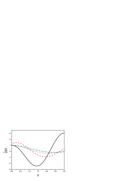
Figure 1: Transverse distributions $\bar{\chi}(y)$ with different values of $c_{1}$ and when $0<c_{1}\leq 1$, $K_{2}$ is fixed to be $1$. The solid line, the dashed line, the dotted line and the dash-dot line are for $c_{1}=0.2$, $0.8$, $1.2$ and $1.8$, respectively.

Some discussions about the solution (56) for the transverse momentum dependence of the B-meson WFs are in the following.

From the solutions in Eqs.(55, 56), one may find that the WFs depend on $c_{2}$ and $c_{3}$ only in a combined form, so the $(c_{2}c_{3})$ in practice stands as one free parameter and hereafter, we shall always replace $(4c_{2}c_{3})$ by merely $c_{3}$ for convenience.

When $c_{1}=1$ and $c_{3}=0$, we return to the transverse momentum dependence of the B-meson wavefunction in the WW approximation. The term including $c_{3}$ brings some differences to the distribution under the WW approximation, especially the allowed range for $\omega$ will be broadened for negative value of $c_{3}$.

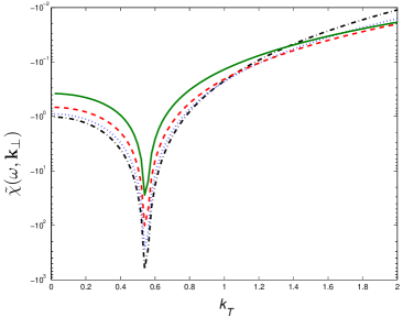
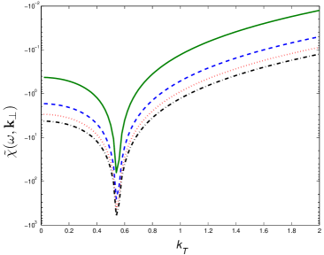
Figure 2: Transverse distributions of $\tilde{\chi}(\omega,\mathbf{k}_{\perp})$ ($k_{T}=|\mathbf{k}_{\perp}|$) with fixed $\bar{\Lambda}=0.55GeV$ and $\omega=0.5GeV$. The left diagram is drawn with fixed $K_{2}=1$ and with some different values for $c_{1}$, i.e. $c_{1}=0.2$, $0.4$, $0.6$ and $0.8$, which are shown in dash-dot, dotted, dashed and solid lines respectively. The right diagram is drawn with fixed $c_{1}=0.6$ and different values for $K_{2}$, i.e. $K_{2}=0$, $5.0$, $10.0$ and $15.0$, which are shown in solid, dashed, dotted and dash-dot lines respectively.

When $c_{1}\geq 1$, one may find the transverse momentum distribution of the B-meson WF tends to be a $\delta$ function as the case in the WW approximation. However, when $0<c_{1}<1$, the transverse momentum distribution of the B-meson WF will be broadened. This is in agreement with the conclusion drawn in Ref.qiao that the 3-particle contributions might considerably broaden the B-meson transverse momentum distribution. To show this point more clearly, we take $c_{3}=0$ and transform the transverse part of Eq.(56) into the momentum space. For $c_{1}\in(0,1)$, we obtain

$$\tilde{\chi}(\omega,\mathbf{k}_{\perp})=-\left(\frac{1}{\Gamma[1-c_{1}]\pi}+\frac{\Gamma[2-c_{1}]\sin[\pi c_{1}]}{\pi^{2}}K_{2}\right)\frac{\Gamma[2-c_{1}]}{{((2\bar{\Lambda}-\omega)\omega)}\left|1-\frac{k_{T}^{2}}{(2\bar{\Lambda}-\omega)\omega}\right|^{2-c_{1}}},$$ (58)

where $k_{T}=|\mathbf{k}_{\perp}|$. One may easily find that $\tilde{\chi}(\omega,\mathbf{k}_{\perp})$ satisfies the normalization condition, $\int d^{2}\mathbf{k}_{\perp}\tilde{\chi}(\omega,\mathbf{k}_{\perp})=1$. The transverse distributions of $\tilde{\chi}(\omega,\mathbf{k}_{\perp})$ with fixed $\bar{\Lambda}=0.55\;GeV$ and $\omega=0.5\;GeV$ are shown in Fig.(2). The left diagram of Fig.(2) is drawn with fixed $K_{2}=1$ and with some different choices for the magnitude of $c_{1}$, i.e. $c_{1}=0.2$, $0.4$, $0.6$ and $0.8$. The right diagram of Fig.(2) is drawn with fixed $c_{1}(=0.6)$, and varying $K_{2}$, i.e. $K_{2}=0$, $5.0$, $10.0$ and $15.0$. From Fig.(2), one may find that with the decreasing of $c_{1}$, or increasing of $K_{2}$, the transverse momentum distributions become broader and broader.

From Fig.(2), one may observe that there is a dip in the transverse momentum distributions around $k_{T}=\sqrt{(2\bar{\Lambda}-\omega)\omega}$. It comes from the denominator in Eq.(58). Practically, such a dip will not make any problem, due to the fact that we always need the integrated results, which will be shown in Sec.IV. By taking the negative value of $c_{3}$, the allowed range of $\omega$ will be broadened and it will make a suppression to the singularity in Eq.(58). When summing up all the Fock states’ contributions and taking the RG evolution effects into consideration, one may expect a further suppression to such singularity in the resultant transverse momentum distributions bwaveevolute .

III.3.2 The distribution functions $\phi_{\pm}(\omega)$ with 3-particle Fock states

The solutions for the distributions $\phi_{\pm}(\omega)$ with 3-particle Fock states have been given in Eqs.(20,25,26). However, since the solutions for $\phi^{(g)}_{\pm}(\omega)$ (as shown in Eq.(26)) involves the unknown 3-particle WFs, it can not be used directly. In the following, we shall make an attempt to provide more convenient expressions for $\phi_{\pm}(\omega)$ under the above mentioned assumptions (I,II,III).

We can derive an expression for the sum of $\phi_{\pm}(\omega)$, $\kappa(\omega)=\phi_{+}(\omega)+\phi_{-}(\omega)$, from Eqs.(54,55), which can be expanded in a more convenient form as

$$\kappa(\omega)=c_{4}\times\exp\left[\frac{2\bar{\Lambda}(c_{1}-1)}{(-c_{3})}\omega\right]\times\left(1+\beta\omega\right),$$ (59)

where $c_{4}$ is an overall normalization factor and we have implicitly taken $(-c_{3})>0$, which is reasonable, since the minus sign indicates that the 3-particle WFs will broaden the allowed range of $\omega$ in comparison to that in the WW approximation. Here, $\beta$ is a new phenomenological parameter, which stands for the summed effects of other expansion terms . Further more, the 3-particle source term $I(\omega)$ can be simplified with the help of Eqs.(11,43,44) as

$$I(\omega)=\frac{\lambda_{E}^{2}-\lambda_{H}^{2}}{18\bar{\Lambda}^{6}}\omega(6\bar{\Lambda}^{2}-6\omega\bar{\Lambda}+\omega^{2})\exp\left(-\frac{\omega}{\bar{\Lambda}}\right).$$ (60)

And then the solution for $\phi_{\pm}(\omega)$ can be obtained from Eqs.(23,59):

$$\phi_{+}(\omega) = c_{4}\beta\omega\times\exp\left[\frac{2\bar{\Lambda}(c_{1}-1)}{(-c_{3})}\omega\right]+c_{4}\omega\left(\beta+\frac{2\bar{\Lambda}(c_{1}-1)}{(-c_{3})}\right){\rm Ei}\left[\frac{2\bar{\Lambda}(c_{1}-1)}{(-c_{3})}\omega\right]-K_{1}\omega$$ (61)

$$-\left\{\frac{\lambda_{E}^{2}-\lambda_{H}^{2}}{18\bar{\Lambda}^{5}}\omega\exp\left(-\frac{\omega}{\bar{\Lambda}}\right)(-\omega+5\bar{\Lambda})+\frac{\lambda_{E}^{2}-\lambda_{H}^{2}}{3\bar{\Lambda}^{4}}\omega\;{\rm Ei}\left(-\frac{\omega}{\bar{\Lambda}}\right)\right\}$$

and

$$\phi_{-}(\omega) = c_{4}\times\exp\left[\frac{2\bar{\Lambda}(c_{1}-1)}{(-c_{3})}\omega\right]-c_{4}\omega\left(\beta+\frac{2\bar{\Lambda}(c_{1}-1)}{(-c_{3})}\right){\rm Ei}\left[\frac{2\bar{\Lambda}(c_{1}-1)}{(-c_{3})}\omega\right]+K_{1}\omega$$ (62)

$$+\left\{\frac{\lambda_{E}^{2}-\lambda_{H}^{2}}{18\bar{\Lambda}^{5}}\omega\exp\left(-\frac{\omega}{\bar{\Lambda}}\right)(-\omega+5\bar{\Lambda})+\frac{\lambda_{E}^{2}-\lambda_{H}^{2}}{3\bar{\Lambda}^{4}}\omega\;{\rm Ei}\left(-\frac{\omega}{\bar{\Lambda}}\right)\right\},$$

where $K_{1}$ is an undetermined parameter and the exponential integral function ${\rm Ei}(z)=-\int^{\infty}_{-z}e^{-t}/tdt$. All the terms in the big parenthesis come from the source term $I(\omega)$.

Some discussions about the solutions (61,62) for $\phi_{\pm}(\omega)$ are in the following.

Eqs.(61,62) show that $c_{1}$ and $c_{3}$ are always in a combined form as $\left[\frac{2\bar{\Lambda}(c_{1}-1)}{(-c_{3})}\right]$, so one can only get the combined results for them. When $\omega\to 0$, we have $\phi_{+}(0)=0$ and $\phi_{-}(0)=c_{4}$. Under the condition $c_{3}<0$, one may observe that $c_{1}$ should be less than 1 to ensure that $\phi_{\pm}(\omega)$ is normalizable, which shows that the transverse momentum dependence of the B-meson wavefunction is broadened due to the introduction of 3-particle wavefunctions.

From Eqs.(23, 59), we obtain

$$\omega\phi_{-}(\omega)-2\int_{0}^{\omega}\phi_{-}(\rho)d\rho=\int_{0}^{\omega}[I(\rho)-\kappa(\rho)]d\rho.$$

Numerically, due to the fact that $\lambda_{E}^{2}\sim\lambda_{H}^{2}$, $\int_{0}^{\omega}I(\rho)d\rho<<\int_{0}^{\omega}\kappa(\rho)d\rho$ for $\forall\;\omega>0$, and then one can safely set $I(\omega)=0$, or equivalently $\lambda_{E}^{2}\simeq\lambda_{H}^{2}$.

Under the approximation $\lambda_{E}^{2}\simeq\lambda_{H}^{2}\simeq 2\bar{\Lambda}^{2}/3$, a solution for $\phi_{\pm}(\omega)$ can be directly obtained by substituting Eqs.(61,62) into constraints (35,36,37), i.e.

$$\phi_{+}(\omega)=\frac{\omega}{\omega_{0}^{2}}\exp\left(-\frac{\omega}{\omega_{0}}\right),\;\;\;\phi_{-}(\omega)=\frac{1}{\omega_{0}}\exp\left(-\frac{\omega}{\omega_{0}}\right),$$ (63)

where $\omega_{0}=2\bar{\Lambda}/3$. The undetermined parameters take the following values, $\left[\frac{2\bar{\Lambda}(c_{1}-1)}{(-c_{3})}\right]=-\frac{1}{\omega_{0}}$, $\beta=\frac{1}{\omega_{0}}$, $K_{1}=0$ and $c_{4}=\frac{1}{\omega_{0}}$. Such solution for $\phi_{\pm}(\omega)$ also satisfies the constraint (38), and it agrees well with the model for $\phi_{\pm}(\omega)$ raised by Ref.grozin , where the same approximation $\lambda_{E}^{2}\simeq\lambda_{H}^{2}\simeq 2\bar{\Lambda}^{2}/3$ is adopted in their QCD sum rule analysis.

IV A model for the B-meson WFs and its phenomenological consequences

In the above section, we have derived an approximate expression for the B-meson WFs under the assumptions (I,II,III), in which the 3-particle Fock states’ contributions are included. The transverse momentum dependence of the B-meson WFs is shown in Eq.(56) and the corresponding DAs are shown in Eqs.(61,62).

For the transverse momentum dependence of the 3-particle WFs, our results indicate that when the value of $c_{1}$ is within the range of $(0,1)$, it may be expanded to a hyperbola-like curve as shown in Figs.(1,2), rather than a simple $\delta$-function as is the case of WW approximation. Our solution for $\phi_{\pm}(\omega)$ favors $c_{1}<1$ under the condition that $c_{3}<0$, which is reasonable since it means that the introduction of 3-particle wavefunctions shall broaden the meson’s longitudinal and transverse distributions. This is in agreement with the conclusion drawn in Ref.qiao , where it has been argued that the 3-particle contributions might considerably broaden the B-meson transverse momentum distribution.

The solutions for the B-meson wavefunction in Eqs.(56,61,62) are somewhat complex. Based on the discussions in Sec.III, we propose a simple model for the B-meson wavefunction with 3-particle Fock states’ contributions in the following. For convenience, we write the two normalized B-meson wavefunctions in the compact parameter $b$-space (useful for the $k_{T}$-factorization approach kt ):

$$\Psi_{+}(\omega,b)=\frac{\omega}{\omega_{0}^{2}}\exp\left(-\frac{\omega}{\omega_{0}}\right)\Big{(}\Gamma[\delta]J_{\delta-1}[\kappa]+(1-\delta)\Gamma[2-\delta]J_{1-\delta}[\kappa]\Big{)}\left(\frac{\kappa}{2}\right)^{1-\delta}$$ (64)

and

$$\Psi_{-}(\omega,b)=\frac{1}{\omega_{0}}\exp\left(-\frac{\omega}{\omega_{0}}\right)\Big{(}\Gamma[\delta]J_{\delta-1}[\kappa]+(1-\delta)\Gamma[2-\delta]J_{1-\delta}[\kappa]\Big{)}\left(\frac{\kappa}{2}\right)^{1-\delta},$$ (65)

with $\omega_{0}=2\bar{\Lambda}/3$, $\kappa=\theta(2\bar{\Lambda}-\omega)\sqrt{\omega(2\bar{\Lambda}-\omega)}b$ and $\delta$ is in the range of $(0,1)$. In the above model, $\lambda_{E}^{2}\simeq\lambda_{H}^{2}\simeq 2\bar{\Lambda}^{2}/3$ is adopted, and to short the uncertainties of the model as much as possible, we only take two main phenomenological parameters $\bar{\Lambda}$ and $\delta$ into the definition. Here for the transverse momentum dependence part, the range of $\omega$ is fixed within the range of $(0,2\bar{\Lambda})$ . When $\delta\to 1$, the transverse momentum dependence of the B-meson wavefunction returns to that of the B-meson wavefunction in the WW approximation. In the above definition, the transverse momentum dependence of the B-meson wavefunction is still the like-function of the off-shell energy of the valence quarks and keeps the main features caused by the 3-particle Fock states, i.e. shall broaden the transverse momentum dependence under the WW approximation to a certain degree.

In order to see the phenomenological influence of the 3-particle Fock states’ contributions, we recalculate the $B\to\pi$ transition form factor within the $k_{T}$-factorization approach and show how $\bar{\Lambda}$ and $\delta$ affect the final results. A consistent analysis of the $B\to\pi$ transition form factor within its physical range has been given in Ref.huangwu by taking the WW B-meson wavefunctions defined in Eqs.(21,22). There we shall adopt the same method as that of Ref.huangwu to do the calculations and to short the paper, we shall only list the results, the interested reader may refer to Ref.huangwu for more details of the calculation technology.

Naively, the main property of the $B\to\pi$ transition form factor is determined by the first inverse moment of $\phi_{+}(\omega)$, and one may find from Eq.(38) that $\left(\Lambda^{(g)}_{0}/\Lambda_{0}^{WW}\right)=(\bar{\Lambda}-\lambda_{B})/\lambda_{B}\sim 0.19$, where $\Lambda^{(g)}_{0}$ is the first inverse moment of $\phi^{(g)}_{+}(\omega)$ and $\Lambda_{0}^{WW}$ is that of $\phi^{WW}_{+}(\omega)$. This shows that the 3-particle wavefunctions might be small. In Ref.charng , by studying the $B\to\gamma l\nu$ decay within the perturbative QCD approach, the authors also claims a small 3-particle contributions. More explicitly, in Ref.charng , the 3-particle contributions are estimated by attaching an extra gluon to the internal off-shell quark line, and then $(1/m_{b})$ power suppression is readily induced. In the following, we shall study the uncertainties caused by two parameters $\delta$ and $\bar{\Lambda}$ under the condition that the 3-particle contribution is less than $\pm 20\%$ of that of the WW case, and at the same time give the possible range for $\delta$ and $\bar{\Lambda}$.

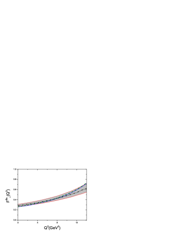
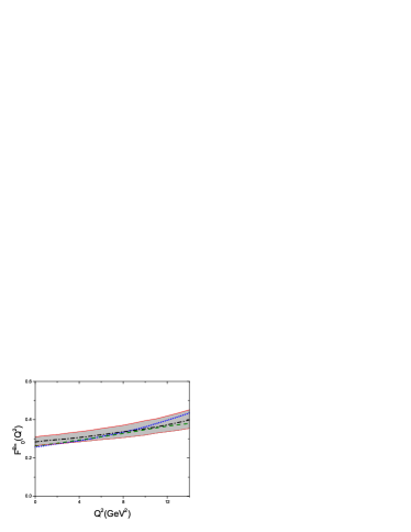
Figure 3: B-meson transition form factors $F^{B\pi}_{+}(Q^{2})$ (Left) and $F^{B\pi}_{0}(Q^{2})$ (Right) with the B-meson wavefunction constructed in Eq.(64,65). The upper (lower) edge of the shaded band is for $\delta=0.30$ ($\delta=0.25$), and the dash-dot line is for $\delta=0.27$. For comparison, the dotted line and the dashed line are for the fitted QCD light cone sum rule results sumrule and the result derived with WW B-meson wavefunction huangwu , respectively. $\bar{\Lambda}=0.55GeV$.

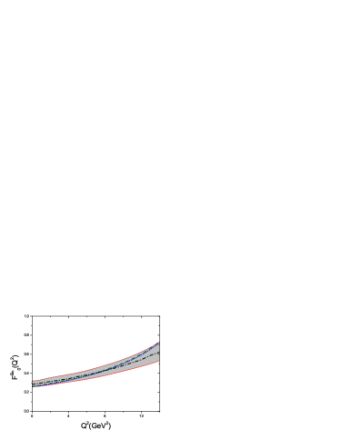
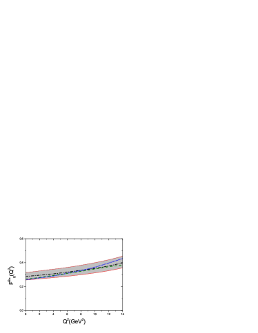
Figure 4: B-meson transition form factors $F^{B\pi}_{+}(Q^{2})$ (Left) and $F^{B\pi}_{0}(Q^{2})$ (Right) with the B-meson wavefunction constructed in Eq.(64,65). The upper (lower) edge of the shaded band is for $\bar{\Lambda}=0.52$ ($\bar{\Lambda}=0.58$), the dash-dot line is for $\bar{\Lambda}=0.55$. For comparison, the dotted line and the dashed line are for the fitted QCD light cone sum rule results sumrule and the result derived with WW B-meson wavefunction huangwu , respectively. $\delta=0.27GeV$.

By taking B-meson wavefunctions as Eqs.(64,65), we first study the uncertainties of $B\to\pi$ transition form factor caused by $\delta$ with fixed $\bar{\Lambda}=0.55GeV$ (the center value of $\bar{\Lambda}$ determined in Ref.huangwu ). We show the $B\to\pi$ transition form factors $F^{B\pi}_{+,0}(Q^{2})$ in Fig.(3). Our results show that if the contribution from the 3-particle wavefunction is limited to be within $\pm 20\%$ of that of WW wavefunction with $Q^{2}\in(0,\sim 10GeV^{2})$, then the value of $\delta$ should be within the region of $(0.25,0.30)$.

Next, we study the uncertainties of $B\to\pi$ transition form factor caused by $\bar{\Lambda}$ with fixed $\delta=0.27$ and the results are shown in Fig.(4). Our results show that if the contribution from the 3-particle wavefunction is limited to be within $\pm 20\%$ of that of WW wavefunction with $Q^{2}\in(0,\sim 10GeV^{2})$, then $\bar{\Lambda}$ should be within the region of $(0.52,0.58)GeV$. Similarly, one may find that if taking a larger value for $\delta$ (e.g. $\delta=0.30$), then the range of $\bar{\Lambda}$ should be shifted to a bigger interval (e.g. $(0.55,0.61)GeV$).

Figs.(3,4) show that by taking into account the 3-particle wavefunctions’ contributions, the $B\to\pi$ transition form factors $F^{B\pi}_{+,0}(Q^{2})$ raise slower with the increment of $Q^{2}$ than the case of WW B-meson wavefunction. And if the contribution from the 3-particle wavefunction is limited to be within $\pm 20\%$ of that of WW wavefunction with $Q^{2}\in(0,\sim 10GeV^{2})$, then the possible range of $\delta$ and $\bar{\Lambda}$ are, $\delta\sim(0.25,0.30)$ and $\bar{\Lambda}\sim(0.50GeV,0.60GeV)$.

V Summary

It had been proved that the B-meson WF is renormalizable after taking into account the RG evolution effects libwave , and the undesirable feature braun of the B-meson DA can be removed under evolution. Therefore, to keep the $k_{T}$ dependence in both the hard scattering amplitude and the wavefunction is necessary. It was found that the transverse and longitudinal momentum dependence in the B-meson WF under the WW approximation is correlated through a $\delta$-function, $\delta(\mathbf{k}_{\perp}^{2}-\omega(2\bar{\Lambda}-\omega))$. In the paper, we show that the transverse momentum distribution of the B-meson WF can be broadened to be a hyperbola-like curve by including 3-particle Fock state, rather than a simple $\delta$-function.

The solutions in this paper provide a practical framework for constructing the B-meson LC WFs $\Psi_{\pm}(\omega,z^{2})$ and hence are meaningful for phenomenological applications. And we have constructed a new model for the B-meson wavefunction in the compact parameter $b$-space as shown in Eqs.(64,65) based on these solutions. There are uncertainties caused by two unknown parameters $\bar{\Lambda}$ and $\delta$. However, since the B-meson WFs are universal, we can determine them by global fitting of the experimental data. By taking $B\to\pi$ transition form factor as an example, we show that if the 3-particle wavefunctions’ contributions are less than $20\%$ of that of the WW case, then one may observe that the preferable values for these two parameters are $\delta\sim 0.27$ and $\bar{\Lambda}\sim 0.55GeV$.

The reasonable inclusion of the 3-particle Fock states in B-meson WFs provides us with the chance to make a more precise evaluation on the B meson decays. Further studies on the B-meson WFs with higher Fock states and its phenomenological implications are still necessary.

Acknowledgements

This work was supported in part by the Natural Science Foundation of China (NSFC). C.-F. Qiao thanks the Institute for Nuclear Theory at the University of Washington for its hospitality and the Department of Energy for partial support during the completion of this work. X.-G. Wu thanks the support from the China Postdoctoral Science Function.

Appendix A Basic formulae for the Fourier transformation

First, we define $\tilde{F}(t,u)=\tilde{F}(t,u,z^{2})|_{z^{2}\to 0}$ and the Fourier transformation:

$$\tilde{\Psi}_{\pm}(t,z^{2}) = \int d\omega\ e^{-i\omega t}\Psi_{\pm}(\omega,z^{2})\ ,$$ (66)

$$\tilde{F}(t,u) = \int d\omega d\xi\ e^{-i(\omega+\xi u)t}F(\omega,\xi).\qquad(F=\{\Psi_{V},\Psi_{A},X_{A},Y_{A}\})$$ (67)

Here $\omega v^{+}$ and $\xi v^{+}$ ($v^{+}$ is the ‘$+$’-component of $v$ defined in Eq.(1)) denote the LC projection of the momentum carried by the light antiquark and the gluon, respectively, and $F(\omega,\xi)$ vanishes unless $\omega\geq 0$ and $\xi\geq 0$.

Some useful formulae:

$$\int\frac{dt}{2\pi}e^{i\omega t}\tilde{\Psi}(t,z^{2}) = \Psi(\omega,z^{2}),$$ (68)

$$\int\frac{dt}{2\pi}e^{i\omega t}\frac{\partial\tilde{\Psi}(t,z^{2})}{\partial t} = -i\omega\Psi(\omega,z^{2}),$$ (69)

$$\int\frac{dt}{2\pi}t^{n}e^{i\omega t}\tilde{\Psi}(t,z^{2}) = (-i)^{n}\frac{\partial^{n}}{\partial\omega^{n}}\Psi(\omega,z^{2}),\qquad(n\geq 1)$$ (70)

$$\int\frac{dt}{2\pi}t^{n}e^{i\omega t}\frac{\partial\tilde{\Psi}(t,z^{2})}{\partial t} = (-i)^{n}\frac{\partial^{n}}{\partial\omega^{n}}[-i\omega\Psi(\omega,z^{2})],\qquad(n\geq 1)$$ (71)

where $\Psi=(\Psi_{+},\Psi_{-})$ and $\tilde{\Psi}=(\tilde{\Psi}_{+},\tilde{\Psi}_{-})$, respectively. And for the 3-particle distributions, we have

$$\int\frac{dudt}{2\pi}e^{i\omega t}\tilde{\Psi}(t,u) = \int_{0}^{\omega}d\rho\int_{\omega-\rho}^{\infty}\frac{d\xi}{\xi}\Psi(\rho,\xi),$$ (72)

$$\int\frac{dudt}{2\pi}t^{n}e^{i\omega t}\tilde{\Psi}(t,u) = (-i)^{n}\frac{\partial^{n}}{\partial\omega^{n}}\int_{0}^{\omega}d\rho\int_{\omega-\rho}^{\infty}\frac{d\xi}{\xi}\Psi(\rho,\xi),\qquad(n\geq 1)$$ (73)

$$\int\frac{ududt}{2\pi}e^{i\omega t}\tilde{\Psi}(t,u) = \int_{0}^{\omega}d\rho\int_{\omega-\rho}^{\infty}\frac{d\xi}{\xi}\left(\frac{\omega-\rho}{\xi}\right)\Psi(\rho,\xi),$$ (74)

$$\int\frac{utdudt}{2\pi}e^{i\omega t}\tilde{\Psi}(t,u) = (-i)\int_{0}^{\omega}d\rho\int_{\omega-\rho}^{\infty}\frac{d\xi}{\xi}\frac{\partial\Psi(\rho,\xi)}{\partial\xi},$$ (75)

$$\int\frac{ut^{n}dudt}{2\pi}e^{i\omega t}\tilde{\Psi}(t,u) = (-i)^{n}\frac{\partial^{n-1}}{\partial\omega^{n-1}}\int_{0}^{\omega}d\rho\int_{\omega-\rho}^{\infty}\frac{d\xi}{\xi}\frac{\partial\Psi(\rho,\xi)}{\partial\xi},\qquad(n\geq 2)$$ (76)

where $\Psi=(\Psi_{V},\Psi_{A},X_{A},Y_{A})$ and $\tilde{\Psi}=(\tilde{\Psi}_{V},\tilde{\Psi}_{A},\tilde{X}_{A},\tilde{Y}_{A})$, respectively. Note here, we have implicitly using the following equation,

$$\int_{0}^{\infty}d\rho\int_{0}^{\infty}d\xi\int_{0}^{1}du\Psi(\rho,\xi)\cdot\delta(\omega-\rho-\xi u)=\int_{0}^{\omega}d\rho\int_{\omega-\rho}^{\infty}\frac{d\xi}{\xi}\Psi(\rho,\xi).$$ (77)

Appendix B Mellin moments of the distribution amplitude

In order to calculate the Mellin moments defined in Eq.(28), it is more convenient to use the derivative of ${\cal G}(\omega)$, i.e.

$$\frac{d}{d\omega}{\cal G}(\omega)=\frac{2\bar{\Lambda}}{\omega(2\bar{\Lambda}-\omega)}\left[I(\omega)+\frac{a_{1}K(\omega)}{2\bar{\Lambda}-\omega}+\frac{a_{2}K(\omega)}{\omega}-a_{2}\frac{d}{d\omega}K(\omega)\right].$$ (78)

And from Eq.(23), we have the following equation,

$$\langle\omega^{n}\rangle_{-}=\frac{\langle\omega^{n}\rangle_{+}}{n+1}-\frac{1}{n+1}\int_{0}^{\infty}\omega^{n}I(\omega)d\omega.$$ (79)

Substituting Eq.(11) into Eq.(79), we get

$$\int_{0}^{\infty}\omega^{n}I(\omega)d\omega = 2\int_{0}^{\infty}\omega^{n}\frac{d}{d\omega}\left[\int_{0}^{\infty}d\rho\int_{0}^{\infty}d\xi\int_{0}^{1}du\frac{\partial}{\partial\xi}[\Psi_{A}-\Psi_{V}]\cdot\delta(\omega-\rho-\xi u)\right]d\omega$$ (80)

$$= -2n\int_{0}^{\infty}d\rho\int_{0}^{\infty}d\xi\int_{0}^{1}du(\rho+\xi u)^{n-1}\frac{\partial}{\partial\xi}[\Psi_{A}-\Psi_{V}]$$

$$= 2n\int_{0}^{\infty}d\rho\int_{0}^{\infty}d\xi\sum_{j=2}^{n}\frac{j-1}{n}{n\choose n-j}\rho^{n-j}\xi^{j-2}[\Psi_{A}-\Psi_{V}]$$

$$= 2n\sum_{j=1}^{n-1}\frac{j}{j+1}{n-1\choose j}[\Psi_{A}-\Psi_{V}]^{n-1}_{j}\ ,$$

where the double moments of the 3-particle distributions are defined as

$$\left[F\right]^{i}_{j}=\int_{0}^{\infty}d\rho\int_{0}^{\infty}d\xi\rho^{i-j}\xi^{j-1}F(\rho,\xi)\qquad(F=\{\Psi_{V},\Psi_{A},X_{A}\})\ .$$ (81)

The moments of $\phi^{(g)}_{+}(\omega)$ can be written as

$$\langle\omega^{n}\rangle^{(g)}_{+} = -\frac{1}{n+2}\int_{0}^{\infty}\frac{\omega^{n+1}}{2\bar{\Lambda}-\omega}\left[I(\omega)+\frac{a_{1}K(\omega)}{2\bar{\Lambda}-\omega}+\frac{a_{2}K(\omega)}{\omega}-a_{2}\frac{d}{d\omega}K(\omega)\right]d\omega$$ (82)

$$+a_{1}\int_{0}^{\infty}\frac{\omega^{n}}{\omega-2\bar{\Lambda}}K(\omega)d\omega\ .$$

More definitely, with the help of the Eqs.(11,12), we have

$$\langle\omega^{n}\rangle^{(g)}_{+} = -\frac{2}{n+2}\int\frac{\omega^{n+1}}{2\bar{\Lambda}-\omega}\frac{d}{d\omega}\left[\int\int\int d\rho d\xi du\frac{\partial}{\partial\xi}[\Psi_{A}-\Psi_{V}]\cdot\delta(\omega-\rho-\xi u)\right]d\omega$$

$$+ \frac{2}{n+2}\int\frac{\omega^{n+1}}{(2\bar{\Lambda}-\omega)^{2}}\left\{\frac{d}{d\omega}\left[\int\int\int d\rho d\xi du[\Psi_{A}+X_{A}]\cdot\delta(\omega-\rho-\xi u)\right]\right.$$

$$\left.\qquad\qquad\qquad\qquad+2\left[\int\int\int d\rho d\xi du\frac{\partial}{\partial\xi}[\Psi_{V}]\cdot\delta(\omega-\rho-\xi u)\right]\right\}d\omega$$

$$+ 2\int\frac{\omega^{n}}{2\bar{\Lambda}-\omega}\left\{\frac{d}{d\omega}\left[\int\int\int d\rho d\xi du[\Psi_{A}+X_{A}]\cdot\delta(\omega-\rho-\xi u)\right]\right.$$

$$\left.\qquad\qquad\qquad\qquad+2\left[\int\int\int d\rho d\xi du\frac{\partial}{\partial\xi}[\Psi_{V}]\cdot\delta(\omega-\rho-\xi u)\right]\right\}d\omega\ ,$$

where we have implicitly applied the relation $a_{1}+a_{2}=1$. To get the final results, the following formulae are useful $(n\geq 2)$,

$$\int_{0}^{\infty}\omega^{n}\frac{d}{d\omega}\left[\int_{0}^{\infty}d\rho\int_{0}^{\infty}d\xi\int_{0}^{1}du\frac{\partial}{\partial\xi}[F]\cdot\delta(\omega-\rho-\xi u)\right]d\omega = n\sum_{j=1}^{n-1}\frac{j}{j+1}{n-1\choose j}[F]^{n-1}_{j}\ ,$$

$$\int_{0}^{\infty}\omega^{n}\frac{d}{d\omega}\left[\int_{0}^{\infty}d\rho\int_{0}^{\infty}d\xi\int_{0}^{1}du[F]\cdot\delta(\omega-\rho-\xi u)\right]d\omega = -\sum_{j=1}^{n}{n\choose j}[F]^{n}_{j}\ ,$$

$$\int_{0}^{\infty}\omega^{n}\left[\int_{0}^{\infty}d\rho\int_{0}^{\infty}d\xi\int_{0}^{1}du\frac{\partial}{\partial\xi}[F]\cdot\delta(\omega-\rho-\xi u)\right]d\omega = -\sum_{j=1}^{n}\frac{j}{j+1}{n\choose j}[F]^{n}_{j}\ ,$$

$$\int_{0}^{\infty}\omega^{n}\frac{d^{2}}{d\omega^{2}}\left[\int_{0}^{\infty}d\rho\int_{0}^{\infty}d\xi\int_{0}^{1}du[F]\cdot\delta(\omega-\rho-\xi u)\right]d\omega = n\sum_{j=1}^{n-1}{n-1\choose j}[F]^{n-1}_{j}\ ,$$

where $F=(\Psi_{V},\Psi_{A},X_{A},Y_{A})$.

With the help of the above formulae, the value of $\langle\omega^{n}\rangle^{(g)}_{+}$ can be directly derived, as is shown in Eq.(30). One subtle point is that, before doing the integration over $\omega$, it is more useful to expand $\frac{1}{2\bar{\Lambda}-\omega}$, i.e.

$$\frac{1}{2\bar{\Lambda}-\omega}=\frac{-1}{\omega}\left(1+\left(\frac{2\bar{\Lambda}}{\omega}\right)+\left(\frac{2\bar{\Lambda}}{\omega}\right)^{2}+\left(\frac{2\bar{\Lambda}}{\omega}\right)^{3}+\cdots\right),$$ (83)

where the power of $\left(\frac{2\bar{\Lambda}}{\omega}\right)$ will be stopped at a particular value, for one may observe that the terms with even higher powers contribute zero exactly. And to do the integration in a form like

$$\int\frac{\omega^{n}}{(\omega-2\bar{\Lambda})^{2}}\frac{d{\cal H(\omega)}}{d\omega}d\omega,$$ (84)

where ${\cal H(\omega)}$ is a function of $\omega$, we can transform it to a more familiar one

$$\int\frac{\omega^{n}}{(\omega-2\bar{\Lambda})^{2}}\frac{d{\cal H(\omega)}}{d\omega}d\omega=n\int\frac{\omega^{n-1}}{(\omega-2\bar{\Lambda})}\frac{d{\cal H(\omega)}}{d\omega}d\omega+\int\frac{\omega^{n}}{(\omega-2\bar{\Lambda})}\frac{d^{2}{\cal H(\omega)}}{d\omega^{2}}d\omega\ .$$ (85)

References

- (1) B.O. Lange and M. Neubert, Phys.Rev.Lett. 91, 102001(2003).
- (2) S. J. Lee and M. Neubert, Phys.Rev. D72, 094028(2005).
- (3) V.M. Braun, D.Y. Ivanov and G.P. Korchemsky, Phys.Rev. D69, 034014(2004).
- (4) B.O. Lange, Eur.Phys.J. C33, S259(2004).
- (5) H. Kawamura, J. Kodaira, C.F. Qiao and K. Tanaka, Phys.Lett. B523, (111)2001, Erratum-ibid. B536, 344 (2002).
- (6) Bodo Geyer and Oliver Witzel, Phys.Rev. D72, 034023(2005).
- (7) A. Khodjamirian, T. Mannel and N. Offen, hep-ph/0504091.
- (8) M. Beneke, T. Feldmann, Nucl.Phys. B592, 3(2001).
- (9) S.D. Genon and C.T. Sachrajda, Nucl.Phys. B625,239(2002).
- (10) H.N. Li and H.S. Liao, Phys.Rev. D70, 074030(2004).
- (11) J. Botts and G. Sterman, Nucl.Phys. B225, 62(1989); H.N. Li and G. Sterman, Nucl.Phys. B381, 129(1992); M. Nagashima and H.N. Li, Phys.Rev. D67, 034001(2003).
- (12) H. Kawamura, J. Kodaira, C.F. Qiao and K. Tanaka, Nucl.Phys. B(Proc.Suppl.)116, 269(2003); Mod.Phys.Lett. A18, 799(2003).
- (13) T. Huang, X.G. Wu and M.Z. Zhou, Phys.Lett.B 611, 260(2005).
- (14) N. Isgur and M.B. Wise Phys. Lett. B232, 113 (1989); N. Isgur and M.B. Wise Phys. Lett. B237, 527(1990); E. Eichten and B. Hill, Phys.Lett. B234, 511(1990).
- (15) S. Wandzura and F. Wilczek, Phys. Lett. B72, 195(1977).
- (16) H. Georgi, Phys.Lett. B240, 447(1990); A.F. Falk, H. Georgi, B. Grinstein and M.B. Wise, Nucl.Phys. B343,1(1990); M. Neubert, Phys. Rept. 245, 259 (1994).
- (17) T. Huang and X.G. Wu, Phys.Rev. D71, 034018(2005).
- (18) T. Huang, Z.H. Li and X.Y. Wu, Phys.Rev. D63, 094001(2001); Z.G. Wang, M.Z. Zhou and T. Huang, Phys.Rev. D67, 094006(2003); P. Ball and R. Zwicky, Phys.Rev. D71, 014015(2005).
- (19) L.D. Debbio, J.M. Flynn, L. Lellouch and J. Nieves, Phys.Lett. B416, 392(1998); D. Becirevic, Nucl.Phys.Proc.Suppl. 94, 337(2001); K.C. Bowler, etal., Phys.Lett. B486, 111(2000).
- (20) A.G. Grozin and M. Neubert, Phys.Rev. D55, 272 (1997).
- (21) T. Huang, in Proceedings of XXth International Conference on High Energy Physics, Madison, Wisconsin, 1980, edited by L.Durand and L.G. Pondrom, AIP Conf.Proc.No. 69(AIP, New York, 1981), p1000; S.J. Brodsky, T. Huang and G.P. Lepage, in Particles and Fields, Vol.2, Proceedings of the Banff Summer Institute, Banff, Alberta, 1981, edited by A.Z. Capri and A.N. Kamal (Plenum, New York, 1983), P143.
- (22) I. Halperin, A. Zhitnitsky, Phys.Rev. D56, 184(1997).
- (23) T. Huang, C.F. Qiao and X.G. Wu, in preparation.
- (24) Y.Y. Charng and H.N. Li, Phys.Rev. D72, 014003(2005).