Secondary pairing in gapless color-superconducting quark matter

We calculate secondary pairing in a model of a color superconductor with a quadratic gapless dispersion relation for the quasiquarks of the primary pairing. Our model mimics the physics of the sector of blue up and red strange quarks in gapless color-flavor-locked quark matter. The secondary pairing opens up a gap $\Delta_{s}$ in the quark spectrum, and we confirm Hong’s prediction that in typical secondary channels $\Delta_{s}\propto G_{s}^{2}$ for coupling strength $G_{s}$. This shows that the large density of states of the quadratically gapless mode greatly enhances the secondary pairing over the standard BCS result $\Delta\propto\exp(-{\rm const}/G)$. In all of the secondary channels that we analyzed we find that the secondary gap, even with this enhancement, is from ten to hundreds of times smaller than the primary gap at reasonable values of the secondary coupling, indicating that secondary pairing does not generically resolve the magnetic instability of the gapless phase.

1 Introduction

The exploration of the phase diagram of matter at ultra-high temperature or density is an area of great interest and activity, both on the experimental and theoretical fronts. Heavy-ion colliders such as the SPS at CERN and RHIC at Brookhaven have probed the high-temperature region, searching for the transition to deconfined quark matter. In this paper we discuss a puzzle that arises in a different part of the phase diagram, at low temperature but ultra-high density. Here there are as yet no experimental constraints, but calculations show that at sufficiently high density, the favored phase is color-flavor-locked (CFL) color-superconducting quark matter [1] (for reviews, see Ref. [2]).

The puzzle concerns the identity of the next phase down in density. Recent work [3] suggests that when the density drops low enough so that the mass of the strange quark can no longer be neglected, there is a continuous phase transition from the CFL phase to a new gapless CFL (gCFL) phase, which could lead to observable consequences if it occurred in the cores of neutron stars [4]. However, it now appears that some of the gluons in the gCFL phase have imaginary Meissner masses, indicating an instability towards an unknown lower-energy phase [5, 6, 7, 8].

The gCFL phase is named after its most striking characteristic: the presence of gapless modes in the spectrum of quark excitations above the color-superconducting ground state. These include a gapless mode with an approximately quadratic dispersion relation $E(p)\propto(p-p_{F})^{2}$, as well as gapless modes with the more typical linear dispersion relation $E(p)\propto|p-p_{F}|$. It seems likely that the presence of these modes is related to the instability. It has therefore been suggested that one way to resolve the instability would be for the gapless quasiparticles to pair with each other (“secondary pairing”), leaving no gapless modes at all. In particular, it has been argued [10] that because the quadratic gapless mode has so much phase space at low energy (its density of states diverges as $E^{-1/2}$) the secondary pairing will be greatly enhanced over the standard BCS value, which is based on pairing of modes that are linearly gapless. This offers the prospect that channels whose attraction seemed negligibly weak could become important once the primary pairing has created a quadratically gapless quasiquark, and these channels could then supply the required secondary pairing. It must be remembered, however, that in order to fully resolve the instability the secondary pairing gap parameter $\Delta_{s}$ must be comparable to the primary pairing $\Delta_{p}$. If $\Delta_{s}$ were significantly smaller then there would be a temperature range $\Delta_{s}\ll T\ll\Delta_{p}$ in which there was primary pairing but no secondary pairing, and at those temperatures the instability problem would arise again.

In this paper we investigate secondary pairing in a simple two-species model with a Nambu–Jona-Lasinio (NJL) interaction. We previously used a similar model to study the effects of gapless modes on photon and gluon screening masses [9]. Our model is essentially just one sector of the gCFL pairing pattern (the blue-up/red-strange sector), which is where a quadratically gapless quasiquark emerges, after primary pairing between the two species, in the Dirac $C\gamma_{5}$ channel.

The Cooper pairs must have an overall antisymmetric wavefunction, and because the secondary pairing is symmetric in color and flavor (pairing a given species with itself), its Dirac structure must be antisymmetric. We also restrict ourselves to rotationally invariant pairing, which leaves three possible Dirac structures for the secondary pairing: $C$, $C\gamma_{5}$, and $C\gamma_{0}\gamma_{5}$. We give a detailed treatment of secondary pairing in the $C\gamma_{0}\gamma_{5}$ channel, because it is the only one that, for a single color and single flavor, is predicted to be attractive under an NJL interaction based on single gluon exchange (Ref. [11], last 4 lines of Table 2). We work at zero temperature throughout.

Our results confirm the conclusion of Ref. [10] concerning the parametric form of the enhancement of the secondary pairing when it operates on quadratically gapless quasiparticles. We find that for a coupling strength $G_{s}$ in the secondary channel, $\Delta_{s}\propto G_{s}^{2}$ as compared to the BCS result $\Delta_{s}\propto\exp(-C/G_{s})$. This was predicted by Hong [10] (note that our $G_{s}$ should be identified with Hong’s effective interaction strength $\kappa$, not with his “$G_{s}$”). This result can also be understood by a simple argument in the NJL model [12] (see end of section 3).

2 Two-species pairing formalism

Our model contains two species of quark with primary pairing leading to anomalous self-energy

$$\langle\psi_{a}C\gamma_{5}\psi_{b}\rangle_{1PI}=\Delta_{p}(\sigma_{1})_{ab}\ .$$ (2.1)

The secondary pairing that we will discuss in most detail is the Dirac $C\gamma_{0}\gamma_{5}$ channel,

$$\langle\psi_{a}C\gamma_{0}\gamma_{5}\psi_{b}\rangle_{1PI}=\Delta_{s}\delta_{ab}\ .$$ (2.2)

The two-dimensional species space, indexed by $a,b=1,2$, corresponds to the blue-up/red-strange sector of the combined color-flavor space in full QCD. As in the gCFL phase, the primary pairing is between species 1 and species 2, with the form $(1,2)+(2,1)$ given by the Pauli matrix $\sigma_{1}$. It is symmetric in the color-flavor indices (because it is antisymmetric in both color and flavor) and antisymmetric in the Dirac indices. It has spin zero (no spatial indices). The secondary pairing pairs each species with itself, and is also antisymmetric in the Dirac indices, and has spin zero. However it vanishes in the limit of massless quarks [9] because it pairs a left-handed quark with a right-handed quark. (For massless quarks with equal and opposite momenta this corresponds to pairing quarks with parallel spins, which would have to give a spin-1 state.) This means that $C\gamma_{0}\gamma_{5}$ secondary pairing can only occur if at least one of the flavors is massive. Fortunately that is the situation we are interested in, since one of our quarks is light (blue up) and the other is heavier (red strange).

One might ask whether we have missed any important physics by using a model that only represents one sector of the gCFL pairing pattern. For example, there might be secondary pairing in other sectors that could feed back into the gap equations in our sector. However, as we will see below, even within our sector the feedback of the secondary pairing on the primary pairing is negligible, because the secondary pairing is so small, so there is no reason to expect significant contamination from other sectors.

To treat the quark-quark condensation, which violates fermion number and allows quarks to turn into antiquarks, we use Nambu-Gor’kov spinors, which incorporate particles and antiparticles into the same spinor, $(\psi,\bar{\psi}^{T})$. Our fermion fields $\chi$ are therefore 16-dimensional, arising from a tensor product of the 4-dimensional Dirac space, the 2-dimensional color-flavor space, and the Nambu-Gor’kov doubling.

The action for the quarks is

$$A=\frac{1}{2}\int\chi(p)^{\dagger}S^{-1}(p)\chi(p)\,\frac{d^{4}p}{(2\pi)^{4}}\ .$$ (2.3)

The inverse propagator $S^{-1}(p)$ is a $16$ by $16$ matrix:

$$S^{-1}(p_{0},\vec{p})=$$

$$\left(\begin{array}[]{c@{\hspace{0em}}c}(p_{\nu}\gamma_{0}\gamma^{\nu}\!+\!\bar{\mu})\otimes\bm{1}\!-\!\delta\mu\otimes\sigma_{3}\!-\!\gamma_{0}\otimes M&\Delta_{p}C\gamma_{5}\otimes\sigma_{1}\!+\!\Delta_{s}C\gamma_{0}\gamma_{5}\otimes\bm{1}\\ (\Delta_{p}C\gamma_{5}\otimes\sigma_{1}\!+\!\Delta_{s}C\gamma_{0}\gamma_{5}\otimes\bm{1})^{T}&[(p_{\nu}\gamma_{0}\gamma^{\nu}\!-\!\bar{\mu})\otimes\bm{1}\!+\!\delta\mu\otimes\sigma_{3}\!+\!\gamma_{0}\otimes M]^{T}\end{array}\right),$$ (2.6)

where in each tensor product the first factor lives in the Dirac space, and the second factor in the color-flavor space. The two species have an average chemical potential $\bar{\mu}$, and a chemical potential splitting $\delta\mu$ which corresponds to the color and electrostatic potentials that enforce neutrality in the gCFL phase. The quark mass matrix is

$$M=\left(\begin{array}[]{cc}m_{u}&0\\ 0&m_{s}\end{array}\right).$$ (2.7)

We can obtain the 4 branches (each 4-fold degenerate) of the full quark dispersion relation, including the effects of both primary and secondary pairing, by finding the values of the energy $\epsilon(\vec{p})$ at which there is a pole in the full propagator

$$\det S^{-1}(\epsilon(\vec{p}),\vec{p})=0\ .$$ (2.8)

If we index these solutions by a label $\alpha=1\ldots 16$ then the grand canonical potential (or, loosely, the free energy) is

$$\Omega(m_{u},m_{s},\bar{\mu},\delta\mu,\Delta_{p},\Delta_{s})=-\int^{\Lambda}\sum_{\alpha}\Bigl{|}\epsilon_{\alpha}(\vec{p},m_{u},m_{s},\bar{\mu},\delta\mu,\Delta_{p},\Delta_{s})\Bigr{|}\frac{d^{3}p}{(2\pi)^{3}}+\frac{\Delta_{p}^{2}}{G_{p}}+\frac{\Delta_{s}^{2}}{G_{s}}\ .$$ (2.9)

The effective couplings $G_{p}$ and $G_{s}$ are determined by details of the NJL model interaction. In this paper we will simply treat them as parameters. Our aim is to see how the secondary pairing $\Delta_{s}$ depends on the coupling $G_{s}$ in the secondary channel. We do not attempt to use “realistic” values for $G_{s}$ (as might be obtained from commonly used NJL models of QCD) because we will be able to show that for any reasonable value of the secondary coupling (i.e for $G_{s}\lesssim{\textstyle\frac{1}{2}}G_{p}$) the secondary gap is too small to generically resolve the magnetic instability of a gapless phase.

Our procedure is as follows.

1. Choose values of ${\bar{\mu}}$, $m_{u}$, and $m_{s}$ that are appropriate for quark matter in the core of a compact star, and an arbitrary ultra-violet cutoff $\Lambda$, significantly larger than ${\bar{\mu}}$. We used ${\bar{\mu}}=500~{}{\rm MeV}$ with $m_{u}=0$ to 100 MeV, $m_{s}=160$ to $300~{}{\rm MeV}$, and cutoff $\Lambda=800$ or $1000~{}{\rm MeV}$.

2. Choose the desired gap parameter $\Delta_{p}$ for the primary pairing. We varied $\Delta_{p}$ from 25 MeV to 75 MeV. To obtain a given value of $\Delta_{p}$ one must choose a value of the coupling $G_{p}$ so that the free energy has a minimum at that value of $\Delta_{p}$. As we vary $G_{p}$ we must also vary $\delta\mu$ so that quasiparticle dispersion relation after primary pairing is always quadratically gapless. To simplify this process we first do it at $m_{u}=m_{s}=0$, where we simply have to set $\delta\mu=\Delta_{p}$ to obtain quadratically gapless dispersion relations. I.e., we solve the gap equation

   $$\frac{2\Delta_{p}}{G_{p}}=\frac{\partial}{\partial\Delta_{p}}\int^{\Lambda}\sum_{\alpha}\Bigl{|}\epsilon_{\alpha}(p,m_{u}=0,m_{s}=0,\bar{\mu},\delta\mu=\Delta_{p},\Delta_{p},\Delta_{s}=0)\Bigr{|}\frac{d^{3}p}{(2\pi)^{3}}$$ (2.10)

   to obtain $G_{p}$$(m_{s}=0)$. We then turn on the desired value of $m_{s}$, and retune $\delta\mu$ to obtain quadratically gapless dispersion relations. It turns out that if we now use the primary gap equation (including the non-zero $m_{s}$) to determine what value of $G_{p}$ gives the desired primary gap parameter $\Delta_{p}$, the result is only slightly different (by $\lesssim 10\%$, typically) from the value of $G_{p}(m_{s}=0)$. So in our results we actually use $G_{p}(m_{s}=0)$. Note that any “error” in $G_{p}$ is really just a rescaling of $\beta$ in the secondary pairing gap equation (2.2), whose only effect would be to slightly shift the line in Fig. 1.

3. Study how the secondary pairing depends on $G_{s}$. Recall that $G_{p}$ and $G_{s}$ both come from the same underlying NJL interaction with some coupling $G$. They arise from Fierz rearrangements of that interaction, so they are both of order $G$, with different numerical coefficients. It is therefore natural to define the ratio of the secondary to the primary effective coupling strength

   $$\beta=G_{s}/G_{p}\ ,$$ (2.11)

   and to study how $\Delta_{s}$ depends on $\beta$. We expect $\beta\lesssim 1$ since the secondary pairing is by definition weaker than the primary pairing. For the $C\gamma_{0}\gamma_{5}$ secondary channel in a single-gluon-based NJL interaction, $\beta\sim{\textstyle\frac{1}{2}}$ [11]. Our final step is therefore to solve the gap equation for the secondary pairing strength $\Delta_{s}$ as a function of $\beta$,

   $$\frac{2\Delta_{s}}{\beta G_{p}}=\frac{\partial}{\partial\Delta_{s}}\int^{\Lambda}\sum_{\alpha}\Bigl{|}\epsilon_{\alpha}(p,m_{u},m_{s},\bar{\mu},\delta\mu,\Delta_{p},\Delta_{s})\Bigr{|}\frac{d^{3}p}{(2\pi)^{3}}$$ (2.12)

   In principle one should solve coupled gap equations (2.10) and (2.12), but we assume that $\Delta_{s}\ll\Delta_{p}$ so, as we see explicitly below, the back-reaction of the secondary pairing on the primary gap is negligible.

3 Results for the $C\gamma_{0}\gamma_{5}$ channel

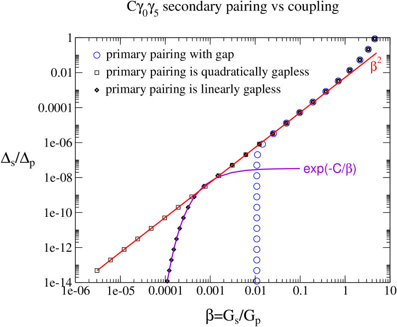
Figure 1: The ratio of the secondary to primary pairing gap parameters $\Delta_{s}/\Delta_{p}$, as a function of the ratio of the coupling strengths in the primary and secondary channels $\beta=G_{s}/G_{p}$. In realistic QCD-like interactions we expect $\beta\lesssim{\textstyle\frac{1}{2}}$, and our original assumption that $\Delta_{s}\ll\Delta_{p}$ turns out to be valid for all $\beta$ in this range. For primary pairing with a quadratically gapless dispersion relation (squares) our results fit $\Delta_{s}\propto\beta^{2}$, as predicted in Ref. [10]. For primary pairing with linearly gapless dispersion relation (small diamonds) we recover the BCS relation $\Delta_{s}\propto\exp(-C/\beta)$ at low $\beta$. If the primary pairing leaves a gap (circles) then secondary pairing disappears at low coupling.

We present detailed results for the case $\bar{\mu}=500~{}{\rm MeV}$, $m_{u}=0$, $m_{s}=300~{}{\rm MeV}$, with cutoff $\Lambda=800~{}{\rm MeV}$. For a primary coupling $G=7.625\times 10^{-6}~{}{\rm MeV}^{-2}$, which gives $\Delta_{p}=75~{}{\rm MeV}$, we tuned $\delta\mu$ to $\delta\mu_{\rm quad}=-26.54544010627093~{}{\rm MeV}$ to obtain quasiquark dispersion relations that were quadratically gapless to within $10^{-13}~{}{\rm MeV}$. We then calculated the secondary pairing as a function of $\beta$. To confirm that the secondary pairing has negligible effect on the primary gap equation, we took the strongest secondary channel coupling, $\beta=1$, which gave $\Delta_{s}=0.555~{}{\rm MeV}$, and re-solved the primary gap equation, including this value of $\Delta_{s}$ in the primary gap equation. This led to a shift $\delta\Delta_{p}=0.003~{}{\rm MeV}$, which is certainly negligible relative to $\Delta_{p}=75~{}{\rm MeV}$. As well as the gapless case, we also studied a slightly less negative value of $\delta\mu$, for which the quasiparticles had a small gap, and a slightly more negative value, for which there were two linearly gapless points. The results are plotted in Fig. 1.

1. Primary pairing giving exactly quadratically gapless quasiquarks (squares in Fig. 1).
   This occurs when $\delta\mu=\delta\mu_{\rm quad}$. Our NJL calculations of the secondary pairing follow the expected result, $\Delta_{s}/\Delta_{p}=A\beta^{2}$ (our fit, straight solid line, is $A=5.287\times 10^{-3}$), all the way down to the lowest secondary couplings that we could probe. Note, however, that in the physically relevant range of couplings, $\beta<1$, the secondary pairing is still suppressed relative to the primary pairing by a factor of 100 or more. (On the straight line fit, $\Delta_{s}/\Delta_{p}(\beta\!=\!1)=A=5.287\times 10^{-3}$).

2. Primary pairing giving gapped quasiquarks (circles in Fig. 1).
   We plot the case $\delta\mu=-26.5454300$, for which the gap in the spectrum is $E_{\rm gap}\approx 10^{-5}~{}{\rm MeV}$. In this case the quasiquark spectrum looks quadratic at higher energies than this (see dashed line in schematic plot of dispersion relations, Fig. 2) and so we expect the secondary pairing will only “notice” the gap if $\Delta_{s}\lesssim 10^{-5}~{}{\rm MeV}$ i.e. $\Delta_{s}/\Delta_{p}\lesssim 10^{-7}$, which corresponds to secondary coupling $\beta\approx 0.01$. The results of the explicit NJL calculation confirm this. For $\beta>0.01$ we obtain a quadratic dependence $\Delta_{s}/\Delta_{p}\propto\beta^{2}$, since the primary quasiquarks look quadratically gapless. At $\beta\approx 0.01$ the secondary pairing falls to zero, since there are no quasiquark modes within $\Delta_{s}$ of the Fermi surface.

3. Primary pairing giving linearly gapless quasiquarks (diamonds in Fig. 1).
   We plot the case $\delta\mu=-26.5454402$, for which the height of the “bounce” in the primary quasiquark dispersion relation is $E_{\rm bounce}\approx 10^{-7}~{}{\rm MeV}$. The quasiquark spectrum looks quadratic at higher energies than this (see dash-dotted line in schematic plot of dispersion relations, Fig. 2), and so we expect the secondary pairing will only “notice” the linearity if $\Delta_{s}\lesssim 10^{-7}~{}{\rm MeV}$, i.e. $\Delta_{s}/\Delta_{p}\lesssim 10^{-9}$, which corresponds to secondary coupling $\beta\approx 0.0003$. The results of the explicit NJL calculation confirm this. For $\beta>0.0003$ we obtain $\Delta_{s}/\Delta_{p}\propto\beta^{2}$, since the primary quasiquarks look quadratically gapless at energies greater that $\Delta_{s}$. At $\beta\approx 0.0003$ the secondary pairing changes to the BCS form, $\Delta_{s}/\Delta_{p}=A\exp(-C/\beta)$ (our fit is $A=3.333\times 10^{-8}$, $C=0.001646$), since the quasiquark modes within $\Delta_{s}$ of the Fermi surface have linear dispersion relations, like those of unpaired fermions.

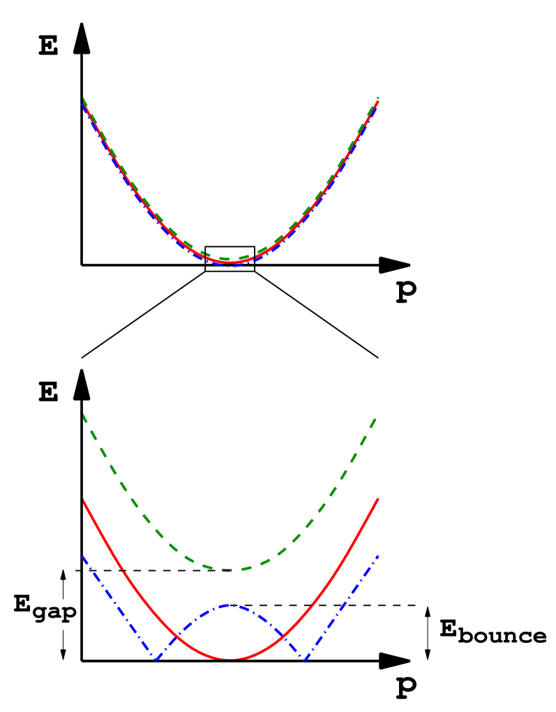
Figure 2: Schematic illustration of the dispersion relations of the quasiquarks (before secondary pairing) that underly the three sets of data plotted in Fig. 1. At higher energy scales, all three dispersion relations look quadratically gapless (upper panel). At energies $\lesssim E_{\rm gap}$ it is possible to distinguish that one case is gapped (dashed line in lower panel). At energies $\lesssim E_{\rm bounce}$ it is possible to distinguish that the other has two linearly gapless points (dash-dotted line in lower panel).

We have checked that the results described above are generic. We have repeated the calculation for values of $m_{s}$ from 160 to 300 MeV, $m_{u}$ from 0 to 100 MeV, and $\Delta_{p}$ from 25 to 75 MeV, for two different values of the cutoff $\Lambda=800$ and 1000 MeV. In every case we found $\Delta_{s}/\Delta_{p}\lesssim 0.01$ at $\beta=1$.

There is a a simple calculation in the NJL formalism, pointed out by K. Rajagopal [12], which shows the origin of Hong’s predicted $\Delta_{s}\propto\beta^{2}$ behavior for quadratically gapless quasiquarks, and moreover enables us to see exactly how the $C\gamma_{0}\gamma_{5}$ gap is suppressed as $m_{s}\to 0$. We first write down the generic form of the gap equation,

$$1=G\int^{\Lambda}\frac{1}{\sqrt{E(p)^{2}+\Delta^{2}}}p^{2}dp\ .$$ (3.13)

In the typical case where the quarks before pairing have linearly gapless dispersion relations $E(p)\propto|p-\mu|$, the integral diverges logarithmically as $\Delta\to 0$, and we obtain the BCS result

$$1\approx G\mu^{2}\log(\Lambda/\Delta)\quad\Rightarrow\quad\Delta\approx\Lambda\exp(-1/(G\mu^{2}))\ .$$ (3.14)

In the case of a quadratically gapless dispersion relation, $E(p)\propto(p-\mu)^{2}/\Delta_{p}$, if we assume (without justification, at this point) that the secondary pairing gap equation also takes the form (3.13), with $\Delta$ replaced by $\Delta_{s}$, then the integral will diverge as an inverse square root of $\Delta_{s}$, so the gap equation for secondary pairing would become (using (2.11))

$$1\propto G_{s}\mu^{2}\sqrt{\Delta_{p}/\Delta_{s}}\quad\Rightarrow\quad\Delta_{s}/\Delta_{p}\propto\mu^{4}G_{p}^{2}\,\beta^{2}\ .$$ (3.15)

which shows the $\Delta_{s}\propto\beta^{2}$ behavior.

The full expression for the integrand on the right-hand-side of the gap equation in the $C\gamma_{0}\gamma_{5}$ channel is very complicated, and we have not been able to find analytic approximations that would reduce it to a simple form that could be compared with (3.13). However, the integrand is dominated by the contribution from the lowest-energy quasiparticle in the range of momenta where it would become quadratically gapless at $\Delta_{s}=0$, and we have numerically evaluated that contribution in the case $m_{u}=0$, and found that it is well approximated (to within about 10% for the values of $\mu,m_{s},\Delta_{p}$ studied in this paper) by

$$\frac{m_{s}^{2}}{2\mu^{2}}\left(\frac{(p-p_{F})^{4}}{\Delta_{p}^{2}}+\frac{m_{s}^{2}}{\mu^{2}}\Delta_{s}^{2}\right)^{-{\textstyle\frac{1}{2}}}\ .$$ (3.16)

If we use this expression in the gap equation, we find

$$1\propto G_{s}\mu^{2}\left(\frac{\Delta_{p}}{\Delta_{s}}\right)^{1/2}\left(\frac{m_{s}}{\mu}\right)^{3/2}\quad\Rightarrow\quad\Delta_{s}/\Delta_{p}\propto m_{s}^{3}\mu G_{p}^{2}\,\beta^{2}\ .$$ (3.17)

This shows both the $\beta^{2}$ dependence, and the $m_{s}^{3}$ suppression of the $C\gamma_{0}\gamma_{5}$ secondary pairing in the limit $m_{s}\to 0$. We have checked the $m_{s}$ dependence by varying $m_{s}$ in our numerical calculations, and found that it is well-described by Eq. (3.17).

For secondary pairing in the other channels that are not suppressed in the $m_{s}\to 0$ limit (such as $C\gamma_{5}$ [10]) the factors of $m_{s}^{2}/\mu^{2}$ in (3.16) would be absent and there would be a prefactor of $\mu^{4}$ instead of $m_{s}^{3}\mu$ in (3.17). For $C\gamma_{0}\gamma_{5}$ self-pairing of a single isolated flavor, as considered in Ref. [11]), where the unpaired quasiparticles have linear dispersion relations, the gap integral has a BCS divergence. In that situation the factors of $m_{s}^{2}/\mu^{2}$ are exponentiated to give a much more severe suppression of the gap as $m_{s}\to 0$, as seen in Fig. 4 of Ref. [11].

4 Other channels

The detailed results presented above are all for condensation of the form $\langle\psi_{a}C\gamma_{0}\gamma_{5}\psi_{b}\rangle_{1PI}=\Delta_{s}\delta_{ab}$, where the single-species pairing has the same sign for both species, $(1,1)+(2,2)$. One could also construct secondary pairing of the form $\langle\psi_{a}C\gamma_{0}\gamma_{5}\psi_{b}\rangle_{1PI}=\Delta_{s}(\sigma_{3})_{ab}$ where the two species each self-pair with opposite sign, $(1,1)-(2,2)$. In Ref. [11] these possibilities were not distinguished because the different colors and flavors were independent of each other. In the current context, however, there is primary pairing in the background, which connects the two species, so that the quasiquarks that undergo secondary pairing are not species eigenstates, but a momentum-dependent superposition of $1$ and $2$. This means that the relative sign of the secondary $(1,1)$ and $(2,2)$ pairing is physically important. We have studied the $C\gamma_{0}\gamma_{5}\,(\sigma_{3})_{ab}$ channel, and we find essentially the same behavior as in the $C\gamma_{0}\gamma_{5}\,\delta_{ab}$ channel: $\Delta_{s}/\Delta_{p}\lesssim 0.01$ for $\beta\lesssim{\textstyle\frac{1}{2}}$ (first line of table 1).

We have also analyzed the other Dirac-antisymmetric channels that are rotational scalars, arbitrarily assigning positive (attractive) interaction strengths $G_{s}$ to these channels. The results are summarized in table 1. For each channel we chose the same parameter values as used in Fig. 1, namely ${\bar{\mu}}=500~{}{\rm MeV}$, $m_{s}=300~{}{\rm MeV}$, $\Delta_{p}=75~{}{\rm MeV}$, $m_{u}=0$, $\Lambda=800~{}{\rm MeV}$, and we tuned $\delta\mu$ to obtain a quadratically gapless quasiquark. In most channels we obtained results similar to those presented in Fig. 1: as the interaction strength drops from 1, $\Delta_{s}/\Delta_{p}$ drops as $\beta^{2}$. The only exception is the $C\delta_{ab}$ channel, where we find that there is no secondary pairing for $\beta\leqslant 1$. However, among the channels studied we find significant variation in the strength of the secondary pairing. The potentially physically relevant region is where the secondary channel interaction strength $G_{s}$ is smaller than the primary channel interaction strength $G_{p}$. In table 1 we therefore show $\Delta_{s}/\Delta_{p}$ at $\beta={\textstyle\frac{1}{2}}$ and 1. We see that in the $C\gamma_{5}(\sigma_{3})_{ab}$ and $C(\sigma_{3})_{ab}$ channels the secondary pairing is about ten times weaker than the primary pairing when $\beta={\textstyle\frac{1}{2}}$, and that in order for $\Delta_{s}$ to be of the same order as $\Delta_{p}$, the secondary channel would have to be as strongly attractive as the primary channel.

Channel	$\Delta_{s}/\Delta_{p}$		Channel	$\Delta_{s}/\Delta_{p}$
	$\beta={\textstyle\frac{1}{2}}$	$\beta=1$		$\beta={\textstyle\frac{1}{2}}$	$\beta=1$
$C\gamma_{0}\gamma_{5}\,\delta_{ab}$	0.0015	0.0074	$C\gamma_{0}\gamma_{5}\,(\sigma_{3})_{ab}$	0.0024	0.012
$C\gamma_{5}\,\delta_{ab}$	0.00019	0.026	$C\gamma_{5}\,(\sigma_{3})_{ab}$	0.093	0.72
$C\,\delta_{ab}$	$<10^{-11}$	$<10^{-11}$	$C\,(\sigma_{3})_{ab}$	$0.067$	$0.53$

Table 1: Secondary pairing in various rotationally-invariant single-species channels. Parameters were the same as in section 3. The secondary channel would have to be as strongly attractive as the primary channel ($\beta=G_{s}/G_{p}=1$) for the secondary pairing to be comparable to the primary pairing. As $\beta$ drops below 1, $\Delta_{s}$ rapidly drops to a small fraction of $\Delta_{p}$.

5 Conclusion

Our results validate the intuition that when the quark dispersion relations (including primary pairing) are quadratically gapless, the very large density of states near the Fermi surface should lead to a parametric enhancement of the secondary pairing, relative to BCS pairing, in weakly coupled channels. However, it is clear that even with this enhancement, the secondary pairing is not typically of comparable magnitude to the primary pairing.

For the case of the $C\gamma_{0}\gamma_{5}$ channel that is predicted to be attractive in single-gluon-exchange-based NJL models, the secondary pairing is at least 100 times weaker than the primary pairing. The other rotationally-invariant secondary channels are predicted to be repulsive ($G_{s}<0$), but we have studied how they would behave if they were attractive. We find that for $G_{s}/G_{p}\leqslant{\textstyle\frac{1}{2}}$, they are at least ten times weaker than the primary pairing. For $G_{s}/G_{p}$ approaching 1 the secondary pairing could become important in certain channels, but that would essentially correspond to assuming that they were not secondary after all, and the competition between the “secondary” and primary channels would have to be taken into account. We therefore conclude that in spite of the great enhancement provided by the large density of states of a quadratically gapless quasiquark, secondary pairing will not generically resolve the magnetic instability of the gapless phase.

This result was obtained under the most favorable conditions for secondary pairing (quadratic gapless dispersion relation), so we expect that it is robust. For example, in full gCFL matter it might turn out that secondary pairing affects the neutrality condition that it is no longer physically correct to tune $\delta\mu$ in the blue-strange/red-up sector so as to obtain a quadratic dispersion relation. However, as is clear from Fig. 1, this can only further suppress the secondary pairing gap. This means that our conclusion will also apply to the (blue-down/green-strange) sector of the gCFL pairing pattern, whose quasiquark is linearly gapless with an energy scale $E_{\rm bounce}\approx\mu_{e}/2$ which is typically tens of MeV. Our results for linearly gapless quasiquarks (diamonds in Fig. 1) show that weakly attractive secondary channels could readily open up a tiny (BCS-suppressed) gap at the linearly gapless points. However, in order to resolve the Meissner instability we would need secondary pairing of the same order as the primary pairing in this sector as well as in the blue-up/red-strange sector. When $\Delta_{s}>E_{\rm bounce}$ the quasiquarks will behave as if they were quadratically gapless, so our analysis also applies to secondary pairing in the blue-down/green-strange sector, and our conclusions apply there as well.

Acknowledgements

We thank K. Rajagopal and D. Hong for useful discussions. This research was supported by the U.S. Department of Energy under grant number DE-FG02-91ER40628.

References

- [1] M. Alford, K. Rajagopal and F. Wilczek, Nucl. Phys. B537, 443 (1999) [hep-ph/9804403].
- [2] K. Rajagopal and F. Wilczek, hep-ph/0011333. M. G. Alford, Ann. Rev. Nucl. Part. Sci. 51 (2001) 131 [hep-ph/0102047]. D. K. Hong, Acta Phys. Polon. B 32, 1253 (2001) [hep-ph/0101025]. D. H. Rischke, Prog. Part. Nucl. Phys. 52, 197 (2004) [nucl-th/0305030]. T. Schäfer, hep-ph/0304281. S. Reddy, Acta Phys. Polon. B 33, 4101 (2002) [nucl-th/0211045].
- [3] M. Alford, C. Kouvaris and K. Rajagopal, Phys. Rev. Lett. 92, 222001 (2004) [hep-ph/0311286]; M. Alford, C. Kouvaris and K. Rajagopal, Phys. Rev. D 71, 054009 (2005) [hep-ph/0406137].
- [4] M. Alford, P. Jotwani, C. Kouvaris, J. Kundu and K. Rajagopal, Phys. Rev. D 71, 114011 (2005) [astro-ph/0411560].
- [5] M. Huang and I. A. Shovkovy, Phys. Rev. D 70, 094030 (2004) [hep-ph/0408268].
- [6] R. Casalbuoni, R. Gatto, M. Mannarelli, G. Nardulli and M. Ruggieri, Phys. Lett. B 605, 362 (2005) [Erratum-ibid. B 615, 297 (2005)] [hep-ph/0410401].
- [7] I. Giannakis and H. C. Ren, Phys. Lett. B 611, 137 (2005) [hep-ph/0412015].
- [8] K. Fukushima, hep-ph/0506080.
- [9] M. Alford and Q.-h. Wang, J. Phys. G 31, 719 (2005) [hep-ph/0501078].
- [10] D. K. Hong, hep-ph/0506097.
- [11] M. G. Alford, J. A. Bowers, J. M. Cheyne and G. A. Cowan, Phys. Rev. D 67, 054018 (2003) [hep-ph/0210106].
- [12] K. Rajagopal, personal communication.