One-loop fermionic corrections to the instanton transition in two dimensional chiral Higgs model

Abstract

The one-loop fermionic contribution to the probability of an instanton transition with fermion number violation is calculated in the chiral Abelian Higgs model in 1+1 dimensions, where the fermions have a Yukawa coupling to the scalar field. The dependence of the determinant on fermionic, scalar and vector mass is determined. We show in detail how to renormalize the fermionic determinant in partial wave analysis, which is convenient for computations.

I Introduction

The interest in the chiral Abelian Higgs model in 1+1 dimensions lies in the fact that it shares some properties with the electroweak theory, but is much simpler and may serve as a toy model. One of the most interesting common features of the two gauge theories is the fermionic number non-conservation thooft . Both give rise to instanton transitions, leading to the creation of a net fermion number due to an anomaly Adler:1969gk ; Bell:1969ts . Both theories contain finite temperature sphaleron transitions Kuzmin:1985mm - Bochkarev:1989vu .

At zero temperature, zero fermionic chemical potentials and for a small number of particles participating in the reaction, the probability of the process can be computed using semi-classical methods. In general, the result is a product of the exponential of the classical action $e^{-S_{cl}}$ and the fluctuation determinants. The latter factor includes the small perturbations of the fields around the instanton configuration, and in many cases may only be computed numerically.

Quite a number of computations of determinants in 1+1 dimensions can be found in the literature. In particular, the determinants have been calculated for the vector and scalar field fluctuations around the instanton in detAphi , as well as for the fermionic ones in detpsim0 , where it was assumed that fermions have no mass term and no interaction with the Higgs field. However, to our best knowledge, no computations incorporating the Yukawa coupling of the fermions to scalar field have been done till now, neither for realistic case of electroweak theory nor for the chiral Abelian Higgs model .

The aim of the present work is to partially fill this gap, calculating the fermionic determinant in the 1+1 dimensional case, where the fermions interact with the Higgs field in a similar way as in the electroweak theory .

This calculation is somewhat delicate because of the difficulties occurring in regularization and renormalization of chiral gauge models beyond perturbation theory. Furthermore, an analytic solution to this problem cannot be obtained, since even the classical instanton profile, given by the Nielsen-Olesen string solution corde , is not known analytically, apart from the special case where the Higgs mass equals the vector field mass cordean . Nevertheless, we use analytical methods as long as possible before moving on to numerical computation. We will use a numerical method developed in BK , extended to our case.

The paper is organized as follows. In section 2, the model and its basic features, such as its vacuum structure, anomaly, instanton configuration and fermionic zero modes are discussed. In section 3, we study and compare the 1-loop divergences occurring in this model in various regularization schemes. In section 4, the method of BK to calculate determinants is discussed and applied to our case. In section 5 we present in some detail the numerical procedures and give the results of the determinant computation. Finally, conclusions are given in section 6.

II The model

The model we consider here contains a complex scalar field $\phi$ with vacuum expectation value $v$; a vector field $A_{\mu}$, and $n_{f}$ fermions $\Psi^{j}$, $j=1,...,n_{f}$:

$$\mathcal{L} = -\frac{1}{4}F^{\mu\nu}F_{\mu\nu}+i\overline{\Psi}^{j}\gamma^{\mu}(\partial_{\mu}-i\frac{e}{2}\gamma^{5}A_{\mu})\Psi^{j}$$ (1)

$$-V(\phi)+\frac{1}{2}\left|D_{\mu}\phi\right|^{2}+if^{j}\overline{\Psi}^{j}\frac{1+\gamma_{5}}{2}\Psi^{j}\phi^{*}-if^{j}\overline{\Psi}^{j}\frac{1-\gamma_{5}}{2}\Psi^{j}\phi.$$

The charges of the left and right-handed fermions differ by a sign, $e_{L}=-e_{R}=\frac{e}{2}$ and the symmetry breaking potential is chosen to be $V[\phi]=\frac{\lambda}{4}(|\phi|^{2}-v^{2})^{2}$. In the following, we use the Majorana representation for the $\gamma$-matrices:

$$\gamma_{0}=\left(\begin{array}[]{cc}0&-i\\ i&0\end{array}\right),\text{ }\gamma_{1}=\left(\begin{array}[]{cc}0&i\\ i&0\end{array}\right),~{}\gamma_{5}=\gamma_{0}\gamma_{1}.$$ (2)

Note that we do not reduce generality in considering Yukawa interaction between identical fermions only. In principle another mass term of the form $M\Psi^{T}\gamma_{0}\Psi+h.\,c.$ could be added to the Lagangian (1). It is compatible with gauge and Lorentz invariance but breaks fermion number explicitly. As we are interested in instanton mediated fermion number non-conservation, we will not consider this term.

This model has been studied as a toy model for the fermionic number non-conservation in the electroweak theory in a number of papers, see, e.g. Grigoriev:1988bd -detAphi , Ringwald .

The particle spectrum consists of a Higgs field with mass $m_{H}^{2}=2\lambda v^{2}$, a vector boson of mass $m_{W}=ev$, and $n_{f}$ Dirac fermions acquiring a mass $F^{j}=f^{j}v$ via Yukawa coupling. The model is free from gauge anomaly. There is, however, a chiral anomaly leading to the non-conservation of the fermionic current,

$$J_{\mu}=J_{\mu}^{L}+J_{\mu}^{R}=\sum_{j=1}^{n_{f}}\overline{\Psi}^{j}_{L}\gamma_{\mu}\Psi^{j}_{L}+\sum_{j=1}^{n_{f}}\overline{\Psi}^{j}_{R}\gamma_{\mu}\Psi^{j}_{R}=\sum_{j=1}^{n_{f}}\overline{\Psi}^{j}\gamma_{\mu}\Psi^{j},$$

with a divergence given by

$$\partial_{\mu}J_{\mu}=\partial_{\mu}J_{\mu}^{L}+\partial_{\mu}J_{\mu}^{R}=-n_{f}\frac{e_{L}}{4\pi}\varepsilon_{\mu\nu}F_{\mu\nu}+n_{f}\frac{e_{R}}{4\pi}\varepsilon_{\mu\nu}F_{\mu\nu}=-n_{f}\frac{e}{4\pi}\varepsilon_{\mu\nu}F_{\mu\nu}.$$ (3)

The vacuum structure of this model is non-trivial Jackiw:1976pf . Taking the $A_{0}=0$ gauge and putting the theory in a spatial box of length $L$ with periodic boundary conditions, one finds that there is an infinity of degenerate vacuum states $|n\rangle,~{}n\in\mathbf{Z}$ with the gauge-Higgs configurations given by

$$A_{1}=\frac{2\pi n}{eL},\quad\phi=ve^{i\frac{2\pi nx}{L}}.$$ (4)

The transition between two neighboring vacua, described by an instanton, leads to the non-conservation of fermion number by $n_{f}$ units. In this paper we consider $n_{f}$ to be even. The case of odd $n_{f}$, resulting in the creation of an odd number of fermions, is analyzed in future .

II.1 Lagrangian in Euclidean space

As the tunneling is best described in Euclidean space-time, we review here the corresponding equations and conventions.

The Lagrangian (1) may be rewritten in Euclidean space:

$$\mathcal{L}^{E} = \frac{1}{4}F_{\mu\nu}F_{\mu\nu}+i\overline{\Psi}^{j}\gamma_{\mu}^{E}(\partial_{\mu}-i\frac{e}{2}\gamma_{5}A_{\mu})\Psi^{j}+V(\phi)$$ (5)

$$+\frac{1}{2}(D_{\mu}\phi)^{\dagger}(D_{\mu}\phi)-if^{j}\overline{\Psi}^{j}\frac{1+\gamma_{5}}{2}\Psi^{j}\phi^{*}+if^{j}\overline{\Psi}^{j}\frac{1-\gamma_{5}}{2}\Psi^{j}\phi,$$

with $D_{\mu}=\partial_{\mu}-ieA_{\mu}$, $\gamma_{0}^{E}=i\gamma_{0}$ and $\gamma_{1}^{E}=\gamma_{1}$. The fields $\overline{\Psi}$ and $\Psi$ are independent variables, and the gauge transformation reads:

$$\Psi \longrightarrow e^{i\alpha(x)\frac{\gamma_{5}}{2}}\Psi\text{ , }\overline{\Psi}\longrightarrow\overline{\Psi}e^{i\alpha(x)\frac{\gamma_{5}}{2}},$$

$$\phi \longrightarrow e^{i\alpha(x)}\phi.$$ (6)

For comparison, the Lorentz transformation is:

$$\Psi(x) \rightarrow \Psi^{\prime}(x^{\prime})=\Lambda_{s}\Psi(\Lambda^{-1}x^{\prime}),$$

$$\overline{\Psi}(x) \rightarrow \overline{\Psi}^{\prime}(x^{\prime})=\overline{\Psi}\Lambda_{s}^{-1}(\Lambda^{-1}x^{\prime}),$$

with $\Lambda_{s}=\exp(i\gamma^{5}\frac{\theta}{2})$ being the rotation matrix in two dimensions.

II.2 Instanton

The instanton which describes the tunneling between the states $|0\rangle$ and $|n\rangle$ is simply the Nielsen-Olesen vortex with winding number $n$ corde , which is a solution of the Euclidean equations of motion in two dimensions. In polar coordinates $(r,~{}\theta)$, the field configuration reads:

$$\phi(r,\theta) = e^{in\theta}\phi(r)=e^{in\theta}vf(r),$$ (7)

$$A^{i}(r,\theta) = \varepsilon^{ij}\widehat{r}^{j}A(r),$$ (8)

where $\widehat{r}$ is the unit vector $\widehat{r}=(\cos\theta,\ \sin\theta)$ and $\varepsilon^{ij}$ the completely antisymmetric tensor with $\varepsilon^{01}=1$. The functions $A$ and $f$ have to satisfy the following limits:

$$f(r)\overset{r\rightarrow 0}{\longrightarrow}cr^{\left|n\right|},$$

$$f(r)\overset{r\rightarrow\infty}{\longrightarrow}1,$$

$$A(r)\overset{r\rightarrow 0}{\longrightarrow}0,$$ (9)

$$A(r)\overset{r\rightarrow\infty}{\longrightarrow}-\frac{n}{er}.$$

Passing to dimensionless variables

$$A=\frac{m}{e}\tilde{A},\quad\phi=\frac{m}{e}\tilde{\phi},\quad r=\frac{\tilde{r}}{m}\quad\text{with}\quad m=\sqrt{\lambda v^{2}}$$ (10)

reduces the number of free parameters. The equations for $\tilde{A},\tilde{\phi}$ are :

$$-\partial_{\tilde{r}}\left(\frac{1}{\tilde{r}}\partial_{\tilde{r}}\tilde{r}\tilde{A}(r)\right)+\tilde{\phi}^{2}\left(\tilde{A}(r)-\frac{1}{\tilde{r}}\right) = 0,$$

$$-\frac{1}{\tilde{r}}\partial_{\tilde{r}}\left(\tilde{r}\partial_{\tilde{r}}\tilde{\phi}(r)\right)+\left(\left(\frac{1}{\tilde{r}}-\tilde{A}(r)\right)^{2}-1+\mu^{2}\tilde{\phi}(r)^{2}\right)\tilde{\phi}(r) = 0,$$ (11)

with $\mu=\frac{m_{H}^{2}}{2m_{W}^{2}}=\frac{\lambda}{e^{2}}$. The classical action is given by:

$$S_{cl} = \pi v^{2}\int_{0}^{\infty}\tilde{r}d\tilde{r}\left\{\mu^{2}\left(\tilde{A}^{\prime}(r)+\frac{\tilde{A}(r)}{\tilde{r}}\right)^{2}\right.$$

$$+ \left.\mu^{2}\left(\tilde{\phi}^{\prime}(r)^{2}+\tilde{\phi}(r)\left(\tilde{A}(r)-\frac{1}{\tilde{r}}\right)^{2}\right)+\frac{\mu^{4}}{2}\left(\tilde{\phi}^{2}(r)-\frac{1}{\mu^{2}}\right)^{2}\right\}.$$

The number $\Delta N$ of fermions created in the instanton transition can be computed by integrating (3) over the Euclidean space:

$$\Delta N=-\int d^{2}x\partial_{\mu}J_{\mu}=-n_{f}\int d^{2}x\frac{e}{4\pi}\varepsilon_{\mu\nu}F_{\mu\nu}=-qn_{f},$$ (13)

where $q=\int d^{2}x\frac{e}{4\pi}\varepsilon_{\mu\nu}F_{\mu\nu}$ is the winding number of the gauge field configuration. For the instanton configuration (7,8), we have $q=n$.

II.3 Fermionic zero modes

According to the index theorem (see for example B ), the Dirac operator in the background of the instanton satisfies the following relation: $\dim\ker[K]-\dim\ker[K^{\dagger}]=n$. As the instanton in 1+1 dimensions coincides with the vortex, these zero modes may be found by carrying out a similar analysis as in jackrossi ; where the fermionic zero modes on the Nielsen-Olesen string were analyzed for non chiral fermions. In this subsection we present the corresponding equations.

The Lagrangian for the fermion $j$ in the background of the scalar and vector fields may be written as $\mathcal{L}^{E}_{f_{j}}=\overline{\Psi}^{j}K^{j}\Psi^{j}$, where

$$K^{j}=\left(\begin{array}[]{cc}-if^{j}\phi^{*}&i\partial_{0}-\frac{e}{2}A_{0}-\partial_{1}-i\frac{e}{2}A_{1}\\ -i\partial_{0}-\frac{e}{2}A_{0}-\partial_{1}+i\frac{e}{2}A_{1}&if^{j}\phi\end{array}\right).$$ (14)

In the following, the family dependent Yukawa coupling $f^{j}$ will be replaced by $f$ keeping in mind that there is no mixing between different fermionic generations.

The zero modes are the regular normalizable solutions of the equation $K\Psi=0$, with $A_{\mu}$ and $\phi$ given by (7,8) . Using polar coordinates and performing the substitution $\tilde{\Psi}=\exp\left[\int_{0}^{r}\frac{A(\rho)}{2}d\rho\right]\Psi$ we get:

$$\left(\begin{array}[]{cc}-iFf(r)e^{-in\theta}&ie^{i\theta}\left(\frac{\partial}{\partial r}+\frac{i}{r}\frac{\partial}{\partial\theta}\right)\\ -ie^{-i\theta}\left(\frac{\partial}{\partial r}-\frac{i}{r}\frac{\partial}{\partial\theta}\right)&iFf(r)e^{in\theta}\end{array}\right)\tilde{\Psi}=0,$$ (15)

where $F=fv$ is the fermion mass. With the use of the phase decomposition $\tilde{\Psi}=\sum_{m=-\infty}^{\infty}e^{im\theta}\Psi^{m}$, equation (15) can be rewritten as

$$Ff(r)\Psi^{m}_{L}-\left(\frac{\partial}{\partial r}-\frac{m-n-1}{r}\right)\Psi_{R}^{m-n-1} = 0,$$

$$\left(\frac{\partial}{\partial r}+\frac{m}{r}\right)\Psi_{L}^{m}-Ff(r)\Psi_{R}^{m-n-1} = 0.$$ (16)

In our case, the analysis of jackrossi shows that for a vortex with topological number $n<0$ there are exactly $|n|$ fermionic zero modes in the spectrum of $K$ with $m$ in the interval $m\in\{-n+1,..,1,0\}$ and none in the spectrum of $K^{\dagger}$. For $n>0$ there are no zero modes in the spectrum of $K$, but $n$ in the spectrum of $K^{\dagger}$.

For the case of $n=-1$ studied below the explicit form of the zero mode is given by

$$\Psi^{0}_{L}(r)=\Psi^{0}_{R}(r)\propto\exp\left(-\int_{0}^{r}\left\{Ff(r^{\prime})+\frac{e}{2}A(r^{\prime})\right\}dr^{\prime}\right).$$ (17)

Note that for massless fermions ($F=0$), the zero mode decreases as $\frac{1}{\sqrt{r}}$ for large $r$. It is therefore not normalizable and has a divergent action. This behavior differ form the case of detpsim0 , Hortacsu:1979fg , Ringwald , where massless fermions of charges $e$ were considered. In their case the fermionic zero mode decreases as $\frac{1}{r}$ for large $r$ and has a finite action.

II.4 Determinant

Due to the presence of the fermionic zero modes, instanton transitions imply the creation of a net number of fermions. In the following, we will be interested in the creation of one of each type of fermion, for which an instanton of charge $n=-1$ is needed. The corresponding transition probability is proportional to ${\mathrm{det}}^{\prime}K$, where the prime means omission of the zero eigenvalue in the calculation of the determinant.

It is well known thooft that the eigenvalue problem for the operator $K$ is ill defined. Consequently one has to consider the Laplacian type operators $K^{\dagger}K$ or $KK^{\dagger}$ which have the same set of eigenvalues (except for the zero modes). Then ${\mathrm{det}}^{\prime}K$ is defined up to a phase as ${\mathrm{det}}^{\prime}[K]={\mathrm{det}}^{\prime}[K^{\dagger}K]^{1/2}$. The explicit expression for the operator $K^{\dagger}K$ reads:

$$K^{\dagger}K=$$ (18)

$$\left[\begin{array}[]{cc}f^{2}|\phi(r)|^{2}-(\partial_{\mu}-i\frac{e}{2}A_{\mu})^{2}+\frac{e}{2}\epsilon_{\mu\nu}\partial_{\mu}A_{\nu}&-if[\phi(eA_{0}+ieA_{1})+(i\partial_{0}-\partial_{1})\phi]\\ if[\phi^{*}(eA_{0}-ieA_{1})-(i\partial_{0}+\partial_{1})\phi^{*}]&f^{2}|\phi(r)|^{2}-(\partial_{\mu}+i\frac{e}{2}A_{\mu})^{2}+\frac{e}{2}\epsilon_{\mu\nu}\partial_{\mu}A_{\nu}\end{array}\right].$$ (21)

The fermionic equations of motion, for instance equation (15), remain unchanged after the variable changes (10), if $f$ is replaced by $f/e$ and $e$ is set to $1$. The only free parameter in the bosonic sector (II.2) is $\mu$, while there is a second parameter in the fermionic sector: the Yukawa coupling $f$.

In conclusion, we are left with two dimensionless parameters, and the determinant can be calculated as a function of

$$\frac{m_{H}}{m_{W}}=\mu\sqrt{2}\quad\text{and}\quad\frac{F}{m_{H}}=\frac{f}{e}\frac{m_{W}}{m_{H}}=\frac{f}{\sqrt{2\lambda}}.$$ (22)

Obviously the determinant, being a product of an infinite number of eigenvalues, is a divergent quantity. In the next section we discuss its regularization and renormalization.

III Regularization and renormalization

For perturbative calculations, the dimensional regularization is best suited. However, as has been observed in thooft , it is not applicable to the computation of the fermionic determinant because the continuation of the instanton fields to a space with fractional number of dimensions is not uniquely defined. Nevertheless, we discuss the dimensional regularization to fix the meaning of the Lagrangian parameters in section 3.1. In section 3.2, we consider another regularization scheme based on partial waves decomposition. It permits to exploit the spherical symmetry and turns out to be convenient for numerical purposes. In appendix A, we consider the Pauli-Villars regularization used in thooft and prove its equivalence with the partial waves procedure.

III.1 Dimensional regularization

The Lagrangian depends on four parameters; the charge $e$, the scalar coupling $\lambda$, the scalar mass $m_{H}$, and the Yukawa coupling $f$. The model under consideration is super-renormalizable. In order to use the dimensional regularization we have to define the $\gamma$-matrices for an arbitrary number $d=2-\varepsilon$ of dimensions:

$$\left\{\gamma^{\mu},\gamma^{\nu}\right\} = 2g^{\mu\nu},$$

$${\mathrm{tr}}(\gamma^{\mu}\gamma^{\nu}) = 2g^{\mu\nu},\quad\mu,\ \nu=0,1,...,d-1.$$ (23)

The definition of the $\gamma^{5}$ matrix is ambiguous, we follow here the usual definition:

$$\left\{\gamma^{5},\gamma^{\nu}\right\} = 0,\quad\nu=0,1.$$

$$\left[\gamma^{5},\gamma^{\nu}\right] = 0,\quad\nu=2,...,d-1.$$ (24)

The physical parameters $e,~{}\lambda,~{}m_{H},~{}f$ in two dimensions are related to the $d$-dimensional parameters $e_{d},~{}\lambda_{d},~{}m_{Hd},~{}f_{d}$ by:

$$e_{d}=e\mu^{1-\frac{d}{2}},\quad\lambda_{d}=\lambda\mu^{2-d},\quad m_{Hd}=m_{H}\mu^{1-\frac{d}{2}},\quad f_{d}=f\mu^{1-\frac{d}{2}}.$$

We will work in the $R_{\xi}$ gauge. The complex field $\phi$ is written as $\phi=v+h+i\varphi$, where $h$ and $\varphi$ are real. The gauge fixing term is

$$\mathcal{L}_{\mathrm{g.f.}}=\frac{1}{2}\int d^{2}x~{}G[A,h,\varphi]^{2},$$ (25)

where

$$G[A,h,\varphi]=\frac{1}{\xi}\left(\partial_{\mu}A^{\mu}-\xi ev\varphi\right).$$ (26)

The Lagrangian for ghost fields $c$ is

$$\mathcal{L}_{\mathrm{ghost}}=\int d^{2}x\bar{c}\left[-\partial^{2}-\xi e^{2}v^{2}\left(1+\frac{h}{v}\right)\right]c.$$ (27)

In the following we will work in the minimal subtraction scheme. The only divergent parameter is the Higgs mass $m_{H}$. A straightforward computation gives the relevant part of the effective action,

$$S^{UV}_{count}=\int d^{d}x\frac{1}{2}\left(\phi^{2}-v^{2}\right)\delta m^{2}$$ (28)

with

$$\delta m^{2}=\frac{1}{4\pi}\left[3\lambda\left\{\ln(\frac{\mu^{2}}{m_{H}^{2}})+\left(\frac{1}{\varepsilon}\right)_{\overline{MS}}\right\}+\left(\lambda-e^{2}\right)\left\{\ln(\frac{\mu^{2}}{m_{W}^{2}})+\left(\frac{1}{\varepsilon}\right)_{\overline{MS}}\right\}\right.$$

$$\left.-2f^{2}\left\{\ln(\frac{\mu^{2}}{F^{2}})+\left(\frac{1}{\varepsilon}\right)_{\overline{MS}}\right\}\right],$$ (29)

where $\left(\frac{1}{\varepsilon}\right)_{\overline{MS}}=\frac{1}{\varepsilon}-\gamma+\ln(4\pi)$. In the minimal subtraction scheme we subtract the counterterm

$$S^{UV}_{count}=\int d^{2}x\frac{1}{2}\left(\phi^{2}-v^{2}\right)\delta m_{\overline{MS}}^{2},$$

with $\delta m_{\overline{MS}}^{2}$ containing all terms in (29) proportional to $\left(\frac{1}{\varepsilon}\right)_{\overline{MS}}$.

For the photon propagator, the bosonic loops do not introduce any renormalization. However, as is well known B , there is a finite contribution coming from fermionic loops. Because of the ambiguities in the definition of $\gamma_{5}$, dimensional regularization breaks the chiral gauge invariance and a term $\frac{e}{4\pi}A_{\mu}^{2}$ needs to be added to the action. The complete counterterm action to be subtracted from the initial action (5) reads:

$$S_{count}=\left\{\int d^{d}x\left(-\frac{e}{4\pi}A_{\mu}^{2}+\frac{1}{2}\left(\phi^{2}-v^{2}\right)\delta m_{\overline{MS}}^{2}\right)\right\}.$$ (30)

III.2 Partial wave regularization

The spherical symmetry of the instanton suggests that partial wave expansion can be used. The eigenvalue problem decouples into one-dimensional differential equations. In this section we discuss a natural way to regularize the partial waves. We consider here only the fermionic sector.

III.2.1 Partial wave expansion

We may write ${\mathrm{det}}[K^{\dagger}K]$ as a path integral:

$${\mathrm{det}}[K^{\dagger}K]=\int\mathcal{D}\eta\mathcal{D}\bar{\eta}\exp\left[\int d^{2}x~{}\bar{\eta}K^{\dagger}K\eta\right].$$ (31)

Partial wave decomposition is defined as follows:

$$\eta(r,\theta)=\sum_{m=-\infty}^{\infty}e^{im\theta}\eta^{m}(r),\quad\bar{\eta}(r,\theta)=\sum_{m=-\infty}^{\infty}e^{-im\theta}\bar{\eta}^{m}(r).$$ (32)

The regularization is done by putting our system in a finite spherical box of radius $R$, and cutting the sum over the partial waves at some $m=L$. After performing the partial wave decomposition, the regularized action reads:

$$S(R,L)=\int_{0}^{R}2\pi r~{}dr\sum_{m,l=-L}^{L}\bar{\eta}^{m}(r)M^{ml}(r)\eta^{l}(r),$$ (33)

with

$$M^{ml}=\frac{1}{2\pi}\int d\theta e^{-im\theta}K^{\dagger}Ke^{il\theta}.$$ (34)

From the general expression (21) for $K^{\dagger}K$, we get for the vacuum:

$$K^{\dagger}K_{vac}=\left[\begin{array}[]{cc}F^{2}-\partial_{0}^{2}-\partial_{1}^{2}&0\\ 0&F^{2}-\partial_{0}^{2}-\partial_{1}^{2}\end{array}\right].$$ (35)

After phase decomposition we obtain a diagonal matrix in both spinor and partial wave space:

$$M^{ml}_{vac}=\delta^{ml}{\rm 1\kern-2.29996ptl}_{2}\left[-\frac{\partial^{2}}{\partial r^{2}}-\frac{1}{r}\frac{\partial}{\partial r}+\frac{m^{2}}{r^{2}}+F^{2}\right],$$ (36)

where ${\rm 1\kern-2.29996ptl}_{2}$ is the identity in spinor space. The radial eigenvalue equation in vacuum reads:

$$M^{mm}_{vac}\eta^{m}_{\lambda}=\lambda^{2}\eta^{m}_{\lambda},$$ (37)

with boundary conditions

$$\eta^{m}(0)=\eta^{m}(R)=0,\quad m\neq 0,$$

$$\eta^{0}(0)=1,\quad\eta^{0}(R)=0.$$ (38)

From the relations (36)-(38) the free propagator may be derived

$$G^{R}_{m}(r,r^{\prime}) = \sum_{\lambda}\frac{\bar{\eta}^{m}_{\lambda}(r)\eta^{m}_{\lambda}(r^{\prime})}{\lambda^{2}}$$ (41)

$$= \frac{{\rm 1\kern-2.29996ptl}}{2\pi}\left\{\begin{array}[]{cc}\frac{I_{m}(Fr)}{I_{m}(FR)}\left[K_{m}(Fr^{\prime})I_{m}(FR)-I_{m}(Fr^{\prime})K_{m}(FR)\right],&\quad r<r^{\prime},\\ \frac{I_{m}(Fr^{\prime})}{I_{m}(FR)}\left[K_{m}(Fr)I_{m}(FR)-I_{m}(Fr)K_{m}(FR)\right],&\quad r>r^{\prime}.\end{array}\right.$$

It allows us to treat the interaction terms present in (21) by standard diagrammatic methods.

III.2.2 One-loop divergences in partial waves

As we have already seen, the fermionic parameter $f$ needs no renormalization. However, the mass of the scalar Higgs receives divergent contributions from fermionic diagrams. The partial wave regularization can’t be introduced at the level of the fermionic Lagrangian (5), but only at the level of the squared determinant (31). One does not expect that the counterterms derived from the initial Lagrangian are sufficient to remove all infinities in (31). Hence, we recalculate the counterterm action (see appendix B for details) needed to renormalize (31). The result is:

$$S_{count}^{UV}(L,R) = \sum_{m=-L}^{L}S^{m}_{count}(R)$$ (42)

$$= \sum_{m=-L}^{L}\int_{0}^{R}2\pi r~{}{\mathrm{tr}}[G^{m}(r,r)]\left(f^{2}\left(|\phi|^{2}-v^{2}\right)+\frac{e}{2}\varepsilon_{\mu\nu}\partial_{\mu}A_{\nu}\right)dr,$$

where the $S^{m}_{count}$ are finite for each $m$ and only the sum is divergent in the limit $L\to\infty$. Note that the counterterm (42) is non-local. This is due to the non-locality of the partial wave regularization procedure and may be checked to be correct by comparison to Pauli-Villars regularization, see appendix A.6.

For small constant background fields, (42) leads to

$$S_{count}^{UV} = \int_{0}^{R}\left(f^{2}\left(|\phi(r)|^{2}-v^{2}\right)+\frac{e}{2}\varepsilon_{\mu\nu}\partial_{\mu}A_{\nu}(r)\right)d^{2}r\frac{1}{2\pi}\left[1+\log\left(\frac{4L^{2}}{F^{2}R^{2}}\right)\right].$$ (43)

In order to get results in the $\overline{MS}$-scheme from those calculated in the partial waves, we calculate the difference $\delta S^{UV}_{count}$ between the effective action found in these two schemes. The result reads

$$\delta S^{UV}_{count}=\left(\log\left(\frac{4L^{2}}{R^{2}\mu^{2}}\right)-\left(\frac{1}{\varepsilon}\right)_{\overline{MS}}\right)\int\frac{d^{2}x}{2\pi}f^{2}(|\phi|^{2}-v^{2})+S_{gf},$$ (44)

where

$$S_{gf}=\log\left(\frac{4L^{2}}{R^{2}F^{2}}\right)\int\frac{d^{2}x}{2\pi}\frac{e}{2}\epsilon_{\nu\rho}\partial_{\nu}A_{\rho}(x).$$ (45)

In comparison with the dimensional regularization, a supplementary divergent term involving gauge fields $S_{gf}$ has appeared. It also arises when using Pauli-Villars scheme (see appendix A.3) and is an extra divergence of the action (31) in comparison to the initial action (5). If we Wick-rotate $S_{gf}$ back to our initial Lagrangian in Minkowski space-time, it gets an extra factor of $i$, the action becomes non-hermitian and breaks unitarity. Because of this, $S_{gf}$ must be subtracted completely.

For the photon propagator, as in dimensional regularization, we have to subtract from the effective action the term

$$S_{count}^{IR}(R)=\frac{e^{2}}{4\pi}\int_{0}^{R}d^{2}rA^{2}(r)$$ (46)

to recover chiral gauge invariance (see appendix B.1).

III.2.3 Regularization and renormalization in partial waves

From the counterterm (43), we see that the initial theory is recovered in the limit $\frac{2L}{FR}\to\infty$. The summation over partial waves and the limit $L\to\infty$ has to be performed first and the infinite volume limit must be taken only after having removed the infrared counterterm.

The explicit expression for the counterterms in the case of space dependent background is obtained in integrating (42) and the renormalized fermionic determinant may formally be written as:

$${\mathrm{det}}_{ren}[K^{\dagger}K]=$$ (47)

$$\lim_{R\to\infty}\left(\lim_{L\to\infty}\left[\prod_{m=-L}^{L}\frac{{\mathrm{det}}[M^{m}_{inst}]}{{\mathrm{det}}[M^{m}_{vac}]}\exp\left\{-S_{count}^{UV}(L,R)\right\}\right]\exp\left\{-S_{count}^{IR}(R)\right\}\right).$$

This prescription differs from the one of BK where the limit $R\to\infty$ is taken first. It is shown in Appendix C that the order of the limits is crucial.

IV Determinant calculation

After the partial wave decomposition (31-34), $K^{\dagger}K(r,\theta)$ was expressed in terms of $M^{lm}(r)$. For our purposes, the case where $M^{lm}$ is diagonal in partial wave space ($M^{lm}=\delta^{m}_{l}M^{m}$) is sufficient. The determinant may be calculated as:

$${\mathrm{det}}[K^{\dagger}K]=\prod_{m=-\infty}^{+\infty}{\mathrm{det}}[M^{m}].$$ (48)

We are left with the much easier problem of finding the determinant of one-dimensional operators, which may be addressed with the following theorem coleman : Let us consider two operators $O_{i}=-\partial_{x}^{2}+W_{i}(x),~{}i=1,2$ defined in an interval of length $R$. Let $\Psi_{i},~{}i=1,2$ be the solution of $O_{i}\Psi_{i}=0$ with the boundary conditions

$$\Psi_{i}(0)=0,\Psi_{i}^{\prime}(0)=1,~{}i=1,2,$$ (49)

we have:

$${\mathrm{det}}\left[\frac{O_{1}}{O_{2}}\right]=\frac{\Psi_{1}(R)}{\Psi_{2}(R)}.$$ (50)

IV.1 Treatment of radial operators

We follow here the method developed in BK to calculate determinants. Note that here we will first consider the radial problem for $0$ to $R$ where $R\gg 1$ and the limit $R\to\infty$ will be taken afterward.

In the present case, even if $M^{ml}$ is diagonal in partial wave space, it is not diagonal in spinor space. The theorem (50) needs generalization to two coupled second order differential equations. We are interested in the ratio between the operator

$$M^{m}=\left(\begin{array}[]{cc}M_{11}^{m}&M_{12}^{m}\\ M_{21}^{m}&M_{22}^{m}\end{array}\right)$$

in the instanton background and the vacuum operator $M^{m,vac}$, which is assumed to be diagonal. Let us define the matrix $\psi^{m}_{ij}$ ($i,j=1,2$) and $\psi^{m,vac}_{L,R}$ as the solutions of the following differential systems:

$$\begin{array}[]{cc}\sum_{j}M^{m}_{ij}\psi^{m}_{j1}=0,&M^{n,vac}_{11}\Psi^{m,vac}_{L}=0,\\ \sum_{j}M_{ij}\psi^{m}_{j2}=0,&M^{n,vac}_{22}\Psi^{m,vac}_{R}=0,\end{array}$$ (51)

with boundary conditions

$$\lim_{r\rightarrow 0}\frac{\psi_{11}^{m}}{\psi^{vac,m}_{L}}=1,\quad\lim_{r\rightarrow 0}\frac{\psi_{21}^{m}}{\psi^{vac,m}_{R}}=0,$$

$$\lim_{r\rightarrow 0}\frac{\psi_{12}^{m}}{\psi^{vac,m}_{L}}=0,\quad\lim_{r\rightarrow 0}\frac{\psi_{22}^{m}}{\psi^{vac,m}_{R}}=1.$$ (52)

The determinant is then given by:

$$\frac{{\mathrm{det}}[M^{m}]}{{\mathrm{det}}[M^{m,vac}]}=\frac{{\mathrm{det}}[\psi_{ij}^{m}(R)]}{\psi^{m,vac}_{L}(R)\psi^{m,vac}_{R}(R)}.$$ (53)

The remaining determinant is just the usual determinant for $2\times 2$ matrices. It is an easy exercise to reproduce step by step the demonstration of coleman in this more general case.

The vacuum operator which is given in (36), has an analytic solution $\Psi^{m,vac}_{j}=I_{m}(Fr)$. For the instanton ($n=-1$) configuration we get:

$$M_{11}^{m} = -\frac{\partial^{2}}{\partial r^{2}}-\frac{1}{r}\frac{\partial}{\partial r}+\frac{m^{2}}{r^{2}}+F^{2}f^{2}(r)+\frac{e}{2}\varepsilon_{\mu\nu}\partial_{\mu}A_{\nu}+\frac{e^{2}}{4}A^{2}(r)+me\frac{A(r)}{r},$$

$$M_{12}^{m} = M_{21}^{m}=F\left(-f^{\prime}(r)-\frac{1}{r}f(r)+eA(r)f(r)\right),$$

$$M_{22} = -\frac{\partial^{2}}{\partial r^{2}}-\frac{1}{r}\frac{\partial}{\partial r}+\frac{m^{2}}{r^{2}}+F^{2}f^{2}(r)+\frac{e}{2}\varepsilon_{\mu\nu}\partial_{\mu}A_{\nu}+\frac{e^{2}}{4}A^{2}(r)-me\frac{A(r)}{r}.$$ (54)

The solution $\Psi_{ij}^{m}(r)$ needs to be computed numerically. To this aim, it is convenient to make the following substitution:

$$\Psi_{ij}^{m}(r)=\left(\delta_{ij}+h_{ij}^{m}(r)\right)I_{m}(r),$$ (55)

The determinant is then evaluated with

$$\frac{{\mathrm{det}}[M^{m}]}{{\mathrm{det}}[M^{vac,m}]}={\mathrm{det}}[\delta_{ij}+h^{m}_{ij}(R)].$$ (56)

In terms of the functions $h^{m}_{ij}$, the equation (51) takes the form of an ordinary quantum mechanical equation with potential $V_{ij}(r)$:

$$\left[\frac{\partial^{2}}{\partial r^{2}}+\left(\frac{1}{r}+2\frac{I_{m}^{\prime}(Fr)}{I_{m}(Fr)}\right)\frac{\partial}{\partial r}\right]h^{m}_{ij}(r)=V_{ik}(r)\left(\delta_{kj}+h^{m}_{kj}(r)\right).$$ (57)

The effective potential $V_{ij}(r)$ in the background of the instanton is given by the following expressions:

$$V_{11}(r) = F^{2}\left(f^{2}(r)-1\right)-e\frac{A(r)}{2r}+e^{2}\frac{A^{2}(r)}{4}-e\frac{A^{\prime}(r)}{2}-me\frac{A(r)}{r},$$

$$V_{12}(r) = V_{21}(r)=eFf(r)A(r)-Ff^{\prime}(r)-\frac{Ff(r)}{r},$$ (58)

$$V_{22}(r) = F^{2}\left(f^{2}(r)-1\right)-e\frac{A(r)}{2r}+e^{2}\frac{A^{2}(r)}{4}-e\frac{A^{\prime}(r)}{2}+me\frac{A(r)}{r}.$$

The functions $h_{ij}^{m}(r)$ can easily be found numerically from (57) with the boundary conditions

$$\begin{array}[]{cc}h_{ij}(0)=0,&i,j=1,2,\\ h^{\prime}_{ij}(0)=0,&i,j=1,2.\end{array}$$ (59)

For $m=0$ we have to remove the zero-mode present in $M^{0}_{inst}$. In this case, it is possible to diagonalize the operator $M^{m}_{inst}$ with the substitution $\Psi_{\pm}=\Psi_{L}\pm\Psi_{R}$:

$$\left[-\frac{\partial^{2}}{\partial r^{2}}-\frac{1}{r}\frac{\partial}{\partial r}+F^{2}f^{2}(r)+\frac{e}{2}\varepsilon_{\mu\nu}\partial_{\mu}A_{\nu}+\frac{e^{2}}{4}A^{2}(r)\right.$$

$$\pm\left.F\left(-f^{\prime}(r)-\frac{1}{r}f(r)+eA(r)f(r)\right)\right]\Psi_{\pm}=M^{0}_{\pm}\Psi_{\pm}=0.$$ (60)

The fermionic zero-mode is contained in $M_{+}^{0}$. We calculate ${\mathrm{det}}[M^{0}_{-}]$ with (50) and ${\mathrm{det}}^{\prime}[M^{0}_{+}]$ as in BK :

$$\frac{{\mathrm{det}}^{\prime}[M^{0,inst}_{+}]}{{\mathrm{det}}[M^{0,vac}_{+}]}=\frac{\frac{d}{d\lambda^{2}}{\mathrm{det}}[M^{0,inst}_{+}+\lambda^{2}]|_{\lambda^{2}=0}}{{\mathrm{det}}[M^{0,vac}_{+}]}=\frac{d}{d\lambda^{2}}h^{\lambda}(R).$$ (61)

In the last relation $h^{\lambda}(r)$ is defined through $\Psi^{inst}_{+\lambda}=\Psi^{vac}(1+h^{\lambda})$ with $\Psi^{inst}_{+\lambda}(r)$ being a solution of

$$(M^{0,inst}_{+}+\lambda^{2})\Psi^{inst}_{+\lambda}(r)=0,$$

with the boundary condition (49) and $\Psi^{vac}(r)=I_{0}(Fr)$ being the solution of

$$M^{0,vac}\Psi^{vac}=0.$$

IV.2 Ultraviolet divergences

A possible way to calculate the counterterms $S_{count}^{m}(R)$ is given in (42). We need to integrate numerically the Green’s function multiplied by the potential $U(r)=f^{2}(|\phi|^{2}-v^{2})+\frac{e}{2}\varepsilon_{\mu\nu}\partial_{\mu}A_{\nu}$. As the Green’s function is not smooth, for numerical calculations, it is more convenient to solve the related differential equation

$$\left[\frac{\partial^{2}}{\partial r^{2}}+\left(\frac{1}{r}+2\frac{I_{m}^{\prime}(Fr)}{I_{m}(Fr)}\right)\frac{\partial}{\partial r}\right]S_{count}^{m}(r)=2U(r),$$ (62)

with the boundary conditions $S_{eff}^{m}(0)=0,~{}S_{eff}^{{}^{\prime}m}(0)=0$. For the instanton configuration we have:

$$U(r)\overset{inst.}{=} F^{2}(f^{2}(r)-1)-\frac{e}{2}(A^{\prime}(r)+\frac{A(r)}{r}).$$ (63)

V Numerical procedures

In this section we describe the numerical methods used in this work. First the background, namely the well known Nielsen-Olesen vortex is considered. The method used here to find the profile is explained briefly. In the second part, the calculations related to the fermionic determinant are discussed, namely the integration of the differential equations, asymptotic solutions, subtraction of divergences and treatment of zero-modes. The renormalization and convergence of the different limits are checked and finally, results for the determinant are given.

V.1 Background

The instanton profile may be found with a shooting method (see for instance NR ). The boundary conditions at $r=0$ are of the form:

$$A(0)=0,\quad A^{\prime}(0)=b,\quad\quad\phi(0)=0,\quad\phi^{\prime}(0)=\beta,$$ (64)

where the parameters $b$ and $\beta$ are found imposing the limits (II.2) and (II.2). We start the numerical integration at $r\sim 10^{-7}$ instead of $r=0$, where some trivial divergences occur, and use a small $r$ expansion for $\phi$ and $A$:

$$A(r) = br-\frac{\beta^{2}}{8}r^{3}+\mathcal{O}(r^{5}),$$

$$\phi(r) = \beta r-\frac{\beta(1+2b)}{8}r^{3}+\mathcal{O}(r^{5}),$$ (65)

valid for $n=-1$. The numerical integration is done with 32 decimals, and to get an accurate profile, the boundary conditions have to be specified within an accuracy of order $\sim 10^{-14}$.

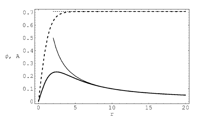
Figure 1: Instanton profile for $m_{H}/m_{W}=2$, classical fields $\phi(r)$ (dashed), $A(r)$ and their asymptotic forms (thin lines).

V.2 Fermionic determinant

For the fermionic determinant, the task is to solve equations (57) and (62). These equations are completely symmetrical under the change $m\rightarrow-m$ therefore only positive $m$ need to be considered. As the solution to the fermionic equations in the asymptotic instanton fields is known, it is sufficient to integrate numerically to $r\sim 15$ and glue the asymptotic solution

$$\Psi_{L}^{m}(r)=AI_{m-1/2}(Fr)+BK_{m-1/2}(Fr),$$

$$\Psi_{R}^{m}(r)=CI_{m+1/2}(Fr)+DK_{m+1/2}(Fr).$$ (66)

The constants $A,~{}B,~{}C,~{}D$ are determined in imposing the continuity of $\Psi^{m}(r)$ and its first derivative. The numerical integration, like for the vortex, starts at $\epsilon\sim 10^{-6}$, where the boundary conditions are found by calculating the power expansion for the $h^{m}_{ij}$:

$$h^{m}_{ij}(\epsilon)=V_{ij}(\epsilon)\frac{\epsilon^{2}\delta_{ij}}{2(2+2m)},\quad h^{\prime m}_{ij}(\epsilon)=V_{ij}(\epsilon)\frac{\epsilon\delta_{ij}}{(2+2m)},$$

$$S^{m}_{count}(\epsilon)=U(\epsilon)\frac{\epsilon^{2}}{2(2+2m)},\quad S^{\prime m}_{count}(\epsilon)=U(\epsilon)\frac{\epsilon}{(2+2m)}.$$ (67)

Having found the $h^{m}_{ij}$, we calculate the partial determinants with (53) and subtract to each wave the partial counterterm $S^{m}_{count}$ found with (62) as prescribed in (47).

Numerically we store the value of the determinant for $\sim 50$ different values of system radius $R_{i},~{}i=1,...,50$.

Figure 2: Logarithm of the partial determinant $\log({\mathrm{det}}[M^{m}])$ as a function of angular momentum $m$, for the parameter values $\frac{m_{H}^{2}}{m_{W}^{2}}=1$, $\frac{F}{m_{H}}=0.1$. The upper small dots shows the results for determinant before renormalization, and the lower ones after. The lines show respectively $1/m$ and $1/m^{2}$ behavior.

After renormalization, the partial determinants ${\mathrm{det}}[M^{m}]$ have to decrease at least as $\frac{1}{m^{2}}$, so that the product over $m$ remains finite. This is checked in figure 2. Using this property, for each $R_{i}$, we calculate the partial determinants from $m=1$ to $m=L\sim 30$ and fit them with an inverse power law:

$${\mathrm{det}}_{ren}[M^{m}]=\frac{const_{2}}{m^{2}}+\frac{const_{3}}{m^{3}}+\frac{const_{4}}{m^{4}}.$$

This approximate expression is then used for $m=L\sim 30$ to infinity.

This completes the limit $L\to\infty$ and we may consider the limit $R\to\infty$. At this point the determinant still depends on $R$ (see figure 3), according to (47), the infrared counterterm (46) have to be subtracted. The renormalized determinant becomes approximately constant for typically $10<FR<100$ and $FR$ can be chosen in this range. Keeping in mind that for large $FR$ higher partial wave should be considered, it is expected that the result becomes inaccurate at large $FR$. Fortunately the determinant converges very fast as $FR\to\infty$ and is found to be constant up to 4 decimals for typically $20<FR<40$ from were the result is extracted.

Figure 3: Logarithm of the determinant $\log({\mathrm{det}}[M])$ as function of the system radius R, before (dashed) and after subtracting the infrared counterterm (46) ($\frac{m_{H}^{2}}{m_{W}^{2}}=1$, $\frac{F}{m_{H}}=0.1$)

For $m=0$ the zero-mode in $M^{0}_{+}$ has to be removed in the determinant calculation. This is done with(61), where the derivative is approximated as

$${\mathrm{det}}^{\prime}[M^{0}_{+}]=\frac{d}{d\lambda^{2}}h^{\lambda}(R)\cong\frac{h^{\lambda}(R)-h^{0}(R)}{\lambda}.$$ (68)

To get an accurate result, we take $\lambda^{2}$ of the order $(10^{-3})F^{2}$ and perform the computation of $h^{\lambda}(R)$ for some $(\sim 10)$ different values of $\lambda$. These results are fitted to extrapolate the value of (68) at $\lambda=0$.

V.3 Results

We first note that ${\mathrm{det}}^{\prime}[M]$ has dimension of $\textrm{mass}^{-2}$ from $\frac{d}{d\lambda^{2}}$ in (61). The fermion mass $F$ may be used to obtain a dimensionless quantity $F^{2}\frac{d}{d\lambda^{2}}{\mathrm{det}}[M]$. The results for $F\sqrt{{\mathrm{det}}^{\prime}[K^{\dagger}K]}$ are plotted in figure 4.

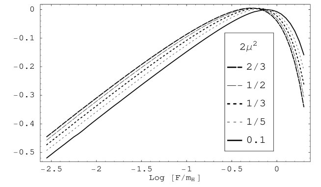
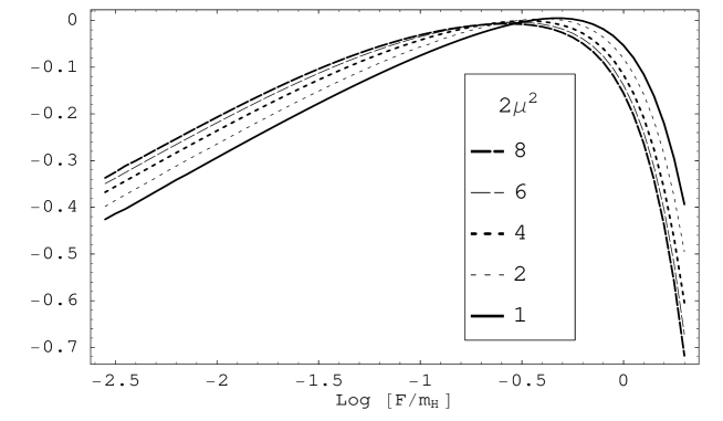
Figure 4: Logarithm of the determinant $\log[F\sqrt{{\mathrm{det}}^{\prime}[K^{\dagger}K]}]$ as a function of the dimensionless fermion mass $\frac{F}{m_{H}}$ (horizontal axis) for different values of $2\mu^{2}=\frac{m_{H}^{2}}{m_{W}^{2}}$. The different values of the determinant are fitted to few percents accuracy with the following expression: $F\sqrt{{\mathrm{det}}^{\prime}[K^{\dagger}K]}=1.62\mu^{1/10}F^{1/4}+\left(-4.60+3.71\mu^{1/5}-0.632\ln\mu\right)F+\left(6.97-6.76\mu^{1/5}+0.866\ln\mu\right)\ln(1+F)$ in the interval $0\leq F\leq 3$ and $0.05\leq\mu^{2}\leq 8$.

The logarithm of the partial determinant $\log({\mathrm{det}}[M^{m}])$ behaves as $\frac{1}{m}$ and after renormalization as $\frac{1}{m^{2}}$, see figure 2. It becomes constant at large $R$ after subtraction of the infrared counterterm, see figure 3.

The behavior of the determinant for small fermion mass $F$ is a power law, see figure 5.

Figure 5: Determinant $F\sqrt{{\mathrm{det}}^{\prime}[K^{\dagger}K]}$ as a function of the dimensionless fermion mass $\frac{F}{m_{H}}$ for the case $\frac{M_{H}}{m_{W}}=1$. The values are fitted with the power law: $F\sqrt{{\mathrm{det}}{M^{0}_{+}}}=1.644\left(\frac{F}{m_{H}}\right)^{1/4}$.

This comes from the partial determinant ${\mathrm{det}}^{\prime}(M^{0}_{+})$ where we remove the zero mode and can be checked with some analytical approximation (see appendix D). The accuracy of the value for the determinant is estimated to be of the order $10^{-3}$ but may be less for $\frac{F}{m_{H}}<10^{-2}$.

$\frac{m_{H}^{2}}{m_{W}^{2}}$	$\frac{S_{cl}}{\pi v^{2}}$	$b$	$\beta$
1/10	0.6388286986270	2.557798983491183	5.756251019029544
1/5	0.7259086109970	1.554461598144364	3.541849174468259
1/3	0.8008642959782	1.081478368993385	2.496453159112955
1/2	0.8679102902678	0.812560321222651	1.901012558603257
2/3	0.9199259150759	0.663981767654766	1.571374124589507
1	1.0000000000000	0.499999999999919	1.206575709162995
2	1.1567609413307	0.308286653343485	0.777359529040461
4	1.3405945494178	0.189926436282935	0.508674018585679
6	1.4612151896139	0.142825844043109	0.399789567459296
8	1.5526758357349	0.116536242666195	0.338046791533589

Table 1: Results for different $\frac{m_{H}^{2}}{m_{W}^{2}}$: classical action ($S_{cl}$), logarithm of the fermionic determinant for dimensionless fermion coupling $g=0.1$ (${\mathrm{det}}_{F=0.1}$) and the boundary conditions at $r=0$ for the instanton profile ($b$ and $\beta$).

VI Conclusion and outlook

In this paper, we have studied an instanton transition in the chiral Abelian Higgs model with fermion number violation and computed the fermionic determinant taking into account the Yukawa couplings.

The dimensional regularization has been used to fix the meaning of the Lagrangian parameters. The numerical calculations have been performed in the partial wave scheme, and the Pauli-Villars regularization is studied for completeness in Appendix A.

In the limit of massless fermion ($F\to 0$), our results can’t be compared to the calculation of detpsim0 , Hortacsu:1979fg , Ringwald . Fermions of electric charge equal to the scalar field charge $e$ where considered in these previous references, whereas we considered pairs of fermions with half-integer charge $\frac{e}{2}$. The instanton transition probability vanishes as $F^{1/4}$ in our case whereas it is finite in the case of integer fermionic charges. As noted in section 2.3, there is no fermionic zero mode in our case if the fermion mass is set to zero. It is therefore not possible to create massless fermions with an instanton of charge $n=-1$. The fact that the probability to create fermions vanishes in the massless limit confirms this observation.

As can be seen in (13), considering only one family of fermions leads to the creation of one single fermion. This process seems to be possible in two dimensions although is it forbidden in four dimensions because of the Witten anomaly Witten . This is an important feature of this model, which is addressed in future .

VII Acknowledgments

We thank F. Bezrukov, S. Khlebnikov, V. Rubakov and P. Tinyakov for helpful discussions. This work has been supported by the Swiss Science Foundation.

Appendix A Appendix: Pauli-Villars regularization

We compare here the Pauli-Villars regularization of thooft to the $\overline{MS}$ regularization and partial wave regularization. The partial wave regularization shows some unusual features such as non-locality, see equation (42), and a renormalization of the gauge field action, see equations (44, 45). In order to understand better their origin, let us compare the partial wave and the well known Pauli-Villars procedure. In Pauli-Villars regularization, a determinant can be calculated as in thooft :

$${\mathrm{det}}_{reg}[K^{\dagger}K_{A,\phi}]=\frac{{\mathrm{det}}[K^{\dagger}K_{A,\phi}]}{{\mathrm{det}}[K^{\dagger}K_{0}]}\frac{{\mathrm{det}}[K^{\dagger}K_{0}+M^{2}]}{{\mathrm{det}}[K^{\dagger}K_{A,\phi}+M^{2}]},$$ (69)

where $K^{\dagger}K_{A,\phi}$ and $K^{\dagger}K_{0}$ are respectively the fermionic operators (21) in the background of the fields $(A,\phi)$ and in the vacuum. In order to determine all necessary counterterms in this regularization scheme, one can consider small perturbations around the vacuum. In principle, the instanton determinant under consideration may have been calculated within Pauli-Villars regularization. However, the partial wave analysis is technically simpler for numerical computations.

A.1 Effective action in Pauli-Villars regularization

The potentially divergent terms may be extracted in calculating the first and second order terms in the Taylor development of the logarithm of (69) with respect to the fields. In the sections A.2, A.3, A.4, we calculate all the relevant functional derivatives and find their contribution to the determinant. The result is the following effective action:

$$S_{count}^{UV} = \log\left(\frac{M^{2}}{F^{2}}\right)\int\frac{d^{2}x}{2\pi}\left\{\frac{e}{2}\epsilon_{\mu\sigma}\partial_{\mu}A_{\sigma}(x)+f^{2}\left(|\phi(x)|^{2}-v^{2}\right)\right\}.$$ (70)

Note that the Pauli-Villars regularization is gauge invariant , however as in the partial waves (45), a new divergent term proportional to $\epsilon_{\mu\sigma}\partial_{\mu}A_{\sigma}$ arises.

To make the link between Pauli-Villars and dimensional regularization in the minimal subtraction scheme, we may calculate the difference $\delta S^{UV}_{count}$ between the effective actions (70) and (28). This provides us with a way to interpret the Pauli-Villars parameter $M$ in terms of the parameter $\mu$ coming from dimensional regularization:

$$\delta S^{UV}_{count}(\mu,M) = \left(\log\left(\frac{M^{2}}{\mu^{2}}\right)-\left(\frac{1}{\varepsilon}\right)_{\overline{MS}}\right)\int\frac{d^{2}x}{2\pi}f^{2}\left(|\phi(x)|^{2}-v^{2}\right)$$ (71)

$$+\log\left(\frac{M^{2}}{F^{2}}\right)\int\frac{d^{2}x}{2\pi}\frac{e}{2}\epsilon_{\nu\sigma}\partial_{\nu}A_{\sigma}(x).$$

The renormalized fermionic determinant ${\mathrm{det}}_{ren}[K^{\dagger}K]$ may be written as:

$${\mathrm{det}}_{ren}[K^{\dagger}K]=\lim_{M\to\infty}\left({\mathrm{det}}_{reg}[K^{\dagger}K]\exp\left\{-S_{count}^{UV}\right\}\right).$$ (72)

The counterterms calculated above can be checked to be sufficient, in calculating determinants of configurations of $A$ and $\phi$ that contains small perturbations around the vacuum. This can be done analytically, see appendix A.5.

A.2 Functional derivatives with respect to the scalar field

We consider first the contributions that lead to the renormalization of the scalar field mass. The corresponding divergent terms can be found in calculating the first and second derivatives of (69) with respect to the scalar field. The first derivatives read:

$$\left.\frac{\delta}{\delta\phi(k)}\log\left({\mathrm{det}}_{reg}[K^{\dagger}K_{A,\phi}]\right)\right|_{A=0,\phi=v}=\left.\frac{\delta}{\delta\phi^{\dagger}(k)}\log\left({\mathrm{det}}_{reg}[K^{\dagger}K_{A,\phi}]\right)\right|_{A=0,~{}\phi=v}$$

$$=f^{2}v\frac{1}{4\pi}\log\left(\frac{M^{2}}{F^{2}}\right)\delta^{2}(k)+\mathcal{O}(M^{-2}),$$ (73)

and their contribution to the logarithm of the determinant is

$$\int\frac{d^{2}k}{(2\pi)^{2}}(\phi(k)-v\delta^{2}(k))\left.\frac{\delta}{\delta\phi(k)}\log\left({\mathrm{det}}_{reg}[K^{\dagger}K_{A,\phi}]\right)\right|_{A=0,\phi=v}+\mathrm{h.~{}c.}$$

$$=\int d^{2}x\left\{v(\phi(x)-v)+v(\phi^{\dagger}(x)-v)\right\}\frac{f^{2}}{2\pi}\log\left(\frac{M^{2}}{F^{2}}\right),$$ (74)

with $\delta^{2}$ the two-dimensional Dirac delta function. The second derivative reads

$$\left.\frac{\delta}{\delta\phi^{\dagger}(q)}\frac{\delta}{\delta\phi(k)}\log\left({\mathrm{det}}_{reg}[K^{\dagger}K(\phi,A)]\right)\right|_{A=0,~{}\phi=v}$$

$$=\frac{f^{2}}{2\pi}\delta(k-q)\log\left(\frac{M^{2}}{F^{2}}\right)+\mathcal{O}(M^{-2}),$$

which gives the following contribution to the logarithm of the determinant:

$$\frac{f^{2}}{2\pi}\int d^{2}x|\phi(x)-v|^{2}\log\left(\frac{M^{2}}{F^{2}}\right).$$

The contribution of the first and second order derivatives can be added to give the second term in (70), which represent a renormalization of the Higgs mass.

A.3 Functional derivatives with respect to the vector field

The first derivative with respect to the vector field

$$\left.\frac{\delta}{\delta A_{\sigma}(k)}\log\left({\mathrm{det}}_{reg}[K^{\dagger}K_{A,\phi}]\right)\right|_{A=0,~{}\phi=v}$$

does not vanish and gives a contribution to the determinant of the form:

$$\frac{e}{2}\log\left(\frac{M^{2}}{F^{2}}\right)\int\frac{d^{2}x}{2\pi}\epsilon_{\mu\sigma}\partial_{\mu}A_{\sigma}(x).$$ (75)

Note that $\int\frac{d^{2}x}{2\pi}\epsilon_{\mu\sigma}\partial_{\mu}A_{\sigma}(x)$ is just the topological charge. For small perturbations around the vacuum with usual boundary conditions (like infinite space and finite energy, see R ), this integral is equal to zero. However this is not true in general and in the present case this integral is equal to $-1$.

A.4 Photon mass term with Pauli-Villars regularization

The regularization procedure we used is gauge invariant. As this is not completely trivial, we shall now check it evaluating the one-loop corrections to the photon propagator. This can be calculated with the second derivative of (69) with respect to $A$ or by evaluating the corresponding Feynman diagrams. Surprisingly, the result, in the limit where the photon momentum $q$ goes to zero reads:

$$\left.\lim_{q^{2}\to 0}\frac{\delta}{\delta A_{\sigma}(k)}\frac{\delta}{\delta A_{\rho}(q)}\log\left({\mathrm{det}}_{reg}[K^{\dagger}K_{A,\phi}]\right)\right|_{A=0,~{}\phi=v} = \frac{e^{2}}{4\pi}\delta_{\mu\nu},$$ (76)

That is we get a mass term for the photon. It is important to note that in chiral gauge theories regularized with a non-gauge invariant procedure, this is a common feature. But here, unlike for instance in dimensional regularization, the regulator term $M^{2}$ is gauge invariant, and such a problem should not arise. Indeed performing further calculations, we can see that every term of the scalar field covariant derivative $|(\partial_{\mu}-ieA_{\mu})\phi|^{2}$ receives a finite contribution from the fermion loop, so that this vector field mass term can be absorbed in a gauge invariant expression. This confirms that Pauli-Villars regularization preserves chiral gauge invariance.

In the remaining of the section, the calculation of the fermionic contribution to photon propagator is presented in more detail. Three diagrams are divergent or constant when the photon momentum goes to zero. We do not present the full calculation by second derivatives of the action but only these three main contributions. The first diagram is the 1-vertex loop with $\frac{e^{2}}{4}A_{\mu}^{2}$ interaction:

(77)

$$= \frac{e^{2}}{4}\frac{\delta_{\mu\nu}}{2\pi}\left[\log\left(\frac{M^{2}}{F^{2}}\right)+\mathcal{O}(M^{-2})\right].$$

The second diagram is the 2-vertexes loop with $-ie\gamma_{5}A_{\mu}\partial_{\mu}$ interaction:

(78)

$$= -\frac{e^{2}}{4}\frac{\delta_{\mu\nu}}{2\pi}\left[\log\left(\frac{M^{2}}{F^{2}}\right)+\mathcal{O}(M^{-2})+\mathcal{O}(q^{2})\right].$$

The integration over $p$ is done by standard techniques. These first two diagrams cancel each other to $\mathcal{O}(M^{-2})+\mathcal{O}(q^{2})$; but the third one gives some constant contribution. Let us consider the 2-vertexes loop with $-ief\phi\gamma_{\mu}A_{\mu}$ interaction; $\phi$ is considered to be in vacuum configuration $\phi=v$ and $fv=F$:

(79)

$$= \frac{e^{2}}{2}\frac{\delta_{\mu\nu}}{2\pi}\left[1+\mathcal{O}(M^{-2})+\mathcal{O}(q^{2})\right].$$

This gives equation (76), which violates at first sight the chiral gauge invariance. Let us consider now other terms involving scalar and vector fields get such contributions, namely $|\partial_{\mu}\phi|^{2}$, $-ieA_{\mu}(\phi^{*}\partial_{\mu}\phi-\phi\partial_{\mu}\phi^{*})$. Let us consider the diagram with two vertexes $f\gamma_{\mu}\partial_{\mu}(\Re(\phi)+i\gamma_{5}\Im(\phi))$:

(80)

$$= \frac{\delta_{\mu\nu}q^{2}}{4\pi v^{2}}+\mathcal{O}(M^{-2})+\mathcal{O}(q^{4}),$$

which gives a contribution

$$\frac{1}{4\pi}\frac{|\partial_{\mu}\phi|^{2}}{v^{2}}$$ (81)

to the effective action. The next diagram is the mixed one and contains one vertex $f\gamma_{\mu}\partial_{\mu}(\Re(\phi)+i\gamma_{5}\Im(\phi))$ and one $-ief\phi\gamma_{\mu}A_{\mu}$; the product of these vertexes gives two terms:

$$2ief^{2}A_{\mu}(\phi^{*}\partial_{\mu}\phi-\phi\partial_{\mu}\phi^{*})+ef^{2}\varepsilon_{\mu\nu}(\phi^{*}\partial_{\mu}\phi+\phi\partial_{\mu}\phi^{*})A_{\nu}.$$

We drop the second one, which is not part of the scalar covariant derivative, and which is gauge invariant (up to total derivative):

(82)

$$= \frac{ie}{2\pi}\frac{i(\delta_{\mu\nu}q_{\nu}+\delta_{\mu\nu}q^{\prime}_{\nu})}{2v^{2}}\left[1+\mathcal{O}(M^{-2})+\mathcal{O}(q^{2})\right],$$

with $q$ the momentum of incoming scalar field $\phi$ and $q^{\prime}$ the out-coming one. This gives a contribution to the scalar-gauge effective action of the form:

$$\frac{ie}{2\pi v^{2}}A_{\mu}(\phi\partial_{\mu}\phi^{*}-\phi^{*}\partial_{\mu}\phi).$$ (83)

It is now possible to resume the terms (76, 81, 83) in a manifestly gauge invariant term $\frac{1}{4\pi v^{2}}|(\partial_{\mu}-ieA_{\mu})\phi|^{2}$ to be added to the initial scalar covariant derivative $\frac{1}{2}|(\partial_{\mu}-ieA_{\mu})\phi|^{2}$ and the photon acquires a mass

$$m_{W}^{1-loop}=\sqrt{e^{2}v^{2}+\frac{e^{2}}{2\pi}}.$$ (84)

This mass can be expressed with the dimensionless parameters (22) as $\frac{m_{w}^{1-loop}}{m_{H}}=\sqrt{\frac{1}{2\mu^{2}}+\frac{1}{4\pi^{2}}}$, which does not depend on the fermion mass. Note that in the case of massless fermions, a similar phenomenon appears (Schwinger mechanism 2dqed ).

A.5 Determinants of small fluctuations

We are checking here if the counterterms mentioned before are sufficient to get a finite determinant. In order to be able to do it analytically we will only consider some small constant perturbation and calculate the ratio of the determinants in (69): First let us take $\phi=v+\delta\phi$, $A=0$, and note that $\delta F=f\delta\phi$:

$$\log\left(\frac{{\mathrm{det}}[K^{\dagger}K(\phi,A)]}{{\mathrm{det}}[K^{\dagger}K_{vac}]}\frac{{\mathrm{det}}[K^{\dagger}K_{vac}+M^{2}]}{{\mathrm{det}}[K^{\dagger}K(\phi,A)+M^{2}]}\right)$$

$$=\log\left(\frac{{\mathrm{det}}[{\rm 1\kern-2.29996ptl}(-\partial_{0}^{2}-\partial_{1}^{2}+(F+\delta F)^{2})]}{{\mathrm{det}}[{\rm 1\kern-2.29996ptl}(-\partial_{0}^{2}-\partial_{1}^{2}+F^{2})]}\frac{{\mathrm{det}}[{\rm 1\kern-2.29996ptl}(-\partial_{0}^{2}-\partial_{1}^{2}+F^{2}+M^{2})]}{{\mathrm{det}}[{\rm 1\kern-2.29996ptl}(-\partial_{0}^{2}-\partial_{1}^{2}+(F+\delta F)^{2}+M^{2})]}\right).$$

In momentum space, we can rewrite the last expression as

$$\left[\int\frac{d^{2}k}{(2\pi^{2})}\log\left(\frac{(k^{2}+(F+\delta F)^{2})^{2}}{(k^{2}+F^{2})^{2}}\frac{(k^{2}+F^{2}+M^{2})^{2}}{(k^{2}+(F+\delta F)^{2}+M^{2})^{2}}\right)\right],$$

which can be easily calculated to give

$$\frac{f^{2}}{2\pi}((v+\delta\phi)^{2}-v^{2})\log\left(\frac{M^{2}}{F^{2}}\right).$$

As the logarithm of the determinant is the sum of all one loop diagrams, we have to make subtractions at this level. Clearly the second term of the counterterm (70) removes the divergence of this determinant. Then if we take $\phi=v$, $A_{\mu}=\delta A_{\mu}$ small constant perturbations; it is easy to perform the same calculations to see that no divergent term occurs. Similarly if we take simultaneously $\phi=v+\delta\phi$ and $A_{\mu}=\delta A_{\mu}$ the calculation is more complicated but we recover once again the previous divergences. However we can see that, taking a specific configuration where $\varepsilon_{\mu\nu}\partial_{\mu}A_{\nu}$ is constant, $\phi=v$ and $A=0$, we find a divergent contribution of the form:

$$\frac{e}{4\pi}\varepsilon_{\mu\nu}\partial_{\mu}A_{\nu}\log\left(\frac{M^{2}}{F^{2}}\right),$$

which is subtracted exactly by the counterterm (75).

A.6 Equivalence between Pauli-Villars and partial wave
counterterms

For small constant background fields we may compare the partial wave counterterm (42) and the Pauli-Villars one (70) The difference $\delta S^{UV}_{count}$ between them relates the different cutoffs $M$ and $\frac{2L}{R}$:

$$\delta S^{UV}_{count}(M,\frac{2L}{R})=\int_{0}^{R}\left(f^{2}\left(|\phi(r)|^{2}-v^{2}\right)+\frac{e}{2}\varepsilon_{\mu,\nu}\partial_{\mu}A_{\nu}(r)\right)d^{2}r\frac{1}{2\pi}\left[1+log\left(\frac{4L^{2}}{M^{2}R^{2}}\right)\right].$$

For any background that approach vacuum at infinity, it can be shown that the Pauli-Villars counterterms are equivalent to the partial wave ones. We introduce a Pauli-Villars regulator in the partial wave counterterm (42):

$$\sum_{m=-L}^{L}\int_{0}^{R}2\pi r{\mathrm{tr}}[G_{F}^{m}(r,r)]h(r)dr$$

$$=\lim_{M\to\infty}\sum_{m=-L}^{L}\int_{0}^{R}2\pi r~{}\left({\mathrm{tr}}[G_{F}^{m}(r,r)]-{\mathrm{tr}}[G_{M}^{m}(r,r)]\right)h(r)dr$$

with $h(r)=\left(f^{2}\phi^{2}+\frac{e}{2}\varepsilon_{\mu\nu}\partial_{\mu}A_{\nu}\right)$ and $G_{F}$ the Green’s function for a particle of mass $F$ given in equation (41). The sum over $m$ is now convergent and we can take $L\to\infty$. The sum of the Green’s functions reads:

$$\sum_{m=-\infty}^{\infty}\left({\mathrm{tr}}[G_{F}^{m}(r,r)]-{\mathrm{tr}}[G_{M}^{m}(r,r)]\right)=\frac{1}{\pi}\sum_{m=-\infty}^{\infty}\left(I_{m}(Fr)K_{m}(Fr)-I_{m}(Mr)K_{m}(Mr)\right).$$

Note that the second term in the Green’s function (41) can be dropped if the potential decreases fast enough at infinity, which is the case here.

We use the following sum rule for Bessel functions: $\sum_{m=-\infty}^{\infty}I_{m}(Fr)K_{m}(Fr^{\prime})=K_{0}(F(r-r^{\prime}))$, therefore, we rewrite the previous expression with two different radii:

$$= \frac{1}{\pi}\lim_{r^{\prime}\to r}\sum_{m=-\infty}^{\infty}\left(I_{m}(Fr)K_{m}(Fr^{\prime})-I_{m}(Mr)K_{m}(Mr^{\prime})\right)$$

$$= \frac{1}{\pi}\lim_{r^{\prime}\to r}[K_{0}(F(r-r^{\prime}))-K_{0}(M(r-r^{\prime}))].$$

For small r, we have $K_{0}(r)\sim-\ln(r)$ and $[K_{0}(F(r-r^{\prime}))-K_{0}(M(r-r^{\prime}))]=ln\left[\frac{M}{F}\right]$. The limit $r^{\prime}\to r$ is trivial and we get for the whole counterterm:

$$\frac{1}{2\pi}\ln\left[\frac{M^{2}}{F^{2}}\right]\int_{0}^{R}h(r)rdr,$$ (85)

which is precisely the counterterm in the Pauli-Villars scheme (70).

Appendix B One-loop divergences in partial waves

The divergent diagrams studied in the framework of Pauli-Villars regularization, see Appendix A.2, A.3, A.4, can be recalculated with partial waves for a constant background. Their sum is expressed in equation (42) and we perform the integration in the following. We have:

$$G^{m}(r,r)=\frac{{\rm 1\kern-2.29996ptl}}{2\pi}\left(I_{m}(Fr)K_{m}(Fr)-\frac{K_{m}(FR)}{I_{m}(FR)}I_{m}(Fr)^{2}\right),$$ (86)

which may be simplified using asymptotic expansions in order for Bessel functions. As the divergences are coming from large $m$, this approximation takes care of the necessary contributions:

$$I_{m}(Fr) = \frac{1}{\sqrt{2\pi}}\frac{1}{(m^{2}+F^{2}r^{2})^{1/4}}\exp\left[\sqrt{m^{2}+F^{2}r^{2}}-m~{}\mathrm{arcsinh}\left(\frac{m}{Fr}\right)\right],$$

$$K_{m}(Fr) = \sqrt{\frac{2}{\pi}}\frac{1}{(m^{2}+F^{2}r^{2})^{1/4}}\exp\left[-\sqrt{m^{2}+F^{2}r^{2}}+m~{}\mathrm{arcsinh}\left(\frac{m}{Fr}\right)\right].$$ (87)

The second term in the propagator (86) is very small if $R\gg 1$ and can be neglected. If the background is supposed to be constant, it can be taken out of the integral, (42) becomes

$$\left(f^{2}\left(|\phi|^{2}-v^{2}\right)+\frac{e}{2}\varepsilon_{\mu,\nu}\partial_{\mu}A_{\nu}\right)\sum_{m=-L}^{L}\int_{0}^{R}2\pi r\frac{1}{2\pi\sqrt{m^{2}+F^{2}r^{2}}}dr$$ (88)

$$= \left(f^{2}\left(|\phi|^{2}-v^{2}\right)+\frac{e}{2}\varepsilon_{\mu,\nu}\partial_{\mu}A_{\nu}\right)\sum_{m=-L}^{L}\frac{1}{F^{2}}\left(\sqrt{m^{2}+F^{2}r^{2}}-m\right),$$

where the sum can be converted to an integral:

$$\left(f^{2}\left(|\phi|^{2}-v^{2}\right)+\frac{e}{2}\varepsilon_{\mu,\nu}\partial_{\mu}A_{\nu}\right)2\int_{0}^{L}\frac{1}{F^{2}}\left(\sqrt{m^{2}+F^{2}r^{2}}-m\right)dm$$ (89)

$$\simeq \left(f^{2}\left(|\phi|^{2}-v^{2}\right)+\frac{e}{2}\varepsilon_{\mu,\nu}\partial_{\mu}A_{\nu}\right)\frac{R^{2}}{2}\left[1+\log\left(\frac{4L^{2}}{F^{2}R^{2}}\right)\right].$$

rewriting $\left(f^{2}\left(|\phi|^{2}-v^{2}\right)+\frac{e}{2}\varepsilon_{\mu,\nu}\partial_{\mu}A_{\nu}\right)$ as an integral over space lead to (43).

B.1 Photon mass term in partial wave

Finally we recalculate the photon propagator in partial waves. The fermionic contribution to the photon propagator comes from three diagrams. The first one reads

$$\psset{unit=19.91693pt}\begin{pspicture}(0.0pt,0.0pt)(99.58466pt,39.83386pt){\psset{arrowsize=3.98338pt 0.0}\psline{->}(49.79233pt,35.85046pt)(53.77571pt,35.85046pt)}\rput(67.71756pt,11.95015pt){$\frac{e^{2}}{4}$}\rput(49.79233pt,-9.95847pt){$\vec{r}$}\pnode(0.0pt,9.95847pt){M_{1}}\rput(47.80063pt,0.0pt){\psCoil[coilaspect=0,coilheight=2,coilwidth=0.3, linewidth=1pt]{90}{1500}}\rput(51.78401pt,0.0pt){\psCoil[coilaspect=0,coilheight=2,coilwidth=0.3, linewidth=1pt]{-1500}{-90}}{\psset{linearc=0.99583pt,linewidth=1.0pt}\pscurve(49.79233pt,0.0pt)(37.84216pt,25.892pt)(49.79233pt,35.85046pt)(61.74248pt,25.892pt)(49.79233pt,0.0pt)}{\psset{fillstyle=solid,fillcolor=black}\cnode(49.79233pt,0.0pt){1.99168pt}{M_{2}}}\end{pspicture}=\frac{e^{2}}{4}\sum_{m}\int_{0}^{R}2\pi rdrG^{m}(r,r){\mathrm{tr}}({\rm 1\kern-2.29996ptl})A_{\mu}^{2}(r).$$ (90)

This integration is precisely the same as (42), and the result is:

$$\frac{e^{2}}{4}\int_{0}^{R}A^{2}_{\mu}d^{2}r~{}\frac{1}{2\pi}\left[1+\log\left(\frac{4L^{2}}{F^{2}R^{2}}\right)\right].$$ (91)

The second diagram is      with vertices $ie\gamma_{5}A_{\mu}\partial_{\mu}$. In our case, $A_{\mu}\partial_{\mu}=A_{r}\partial_{r}+A_{\theta}\frac{1}{r}\partial_{\theta}$ with $A_{r}=0$ and $\frac{1}{r}\partial_{\theta}$ is replaced by $\frac{m}{r}$ for the partial wave $m$. We further assume that $A_{\theta}$ is constant over all space. The above diagram gives

$$-\frac{1}{2!}e^{2}{\mathrm{tr}}(\gamma_{5}^{2})\sum_{m}\int d^{2}rd^{2}r^{\prime}A_{\theta}\frac{m}{r}G^{m}(r,r^{\prime})A_{\theta}\frac{m}{r^{\prime}}G^{m}(r^{\prime},r),$$ (92)

where $G^{m}(r,r^{\prime})$ is given by (86). We are interested in large $m$ contributions, and therefore we use the asymptotic formulas (B, 87) for Bessel functions in the propagator. We are also interested in the limit $R\gg 1$, therefore we drop once again the second term in the propagator. After some calculations we get :

$$G^{2}(r,r^{\prime})=\frac{1}{4(2\pi)^{2}}\frac{1}{\sqrt{m^{2}+F^{2}r^{2}}}\frac{1}{\sqrt{m^{2}+F^{2}r^{\prime 2}}}\left\{\exp\left[2g(m,r,r^{\prime})\right]\theta(r^{\prime}-r)\right.$$

$$\left.+~{}\exp[2g(m,r^{\prime},r)]\theta(r-r^{\prime})\right\}.$$ (93)

with

$$g(m,r,r^{\prime})=\left(\sqrt{m^{2}+F^{2}r^{2}}-\sqrt{m^{2}+F^{2}r^{\prime 2}}-m\,\mathrm{arcsinh}\frac{m}{Fr}+m\,\mathrm{arcsinh}\frac{m}{Fr^{\prime}}\right).$$

The dominant contribution comes from diagrams with $r\cong r^{\prime}$. Expanding in powers of $r-r^{\prime}$ and performing the integrations, we get for (92):

$$-\frac{e^{2}}{4}A_{\theta}^{2}\sum_{m}\int_{0}^{R}\frac{m^{2}dr}{m^{2}+F^{2}r^{2}}\left\{\int_{r}^{R}dr^{\prime}\exp\left[2\frac{\sqrt{m^{2}+F^{2}r^{2}}(r-r^{\prime})}{r}\right]\right.$$ (94)

$$\left.+\int_{0}^{r}dr^{\prime}\exp\left[2\frac{\sqrt{m^{2}+F^{2}r^{2}}(r^{\prime}-r)}{r}\right]\right\}$$

$$= -\frac{e^{2}}{4}A_{\theta}^{2}\sum^{L}_{m=-L}m^{2}\left[\frac{1}{F^{2}m}-\frac{1}{F^{2}\sqrt{m^{2}+F^{2}R^{2}}}\right]$$

$$\simeq -\frac{e^{2}}{4}A_{\theta}^{2}~{}2\int^{L}_{0}m^{2}\left[\frac{1}{F^{2}m}-\frac{1}{F^{2}\sqrt{m^{2}+F^{2}R^{2}}}\right]dm$$

$$= -\frac{e^{2}}{2}A_{\theta}^{2}\left[\frac{1}{4}R^{2}\left(-1+\log\left(\frac{4L^{2}}{F^{2}R^{2}}\right)\right)+\mathcal{O}(L^{-2})\right]$$

$$\simeq -\frac{e^{2}}{4}\int_{0}^{R}A_{\mu}^{2}d^{2}r~{}\frac{1}{2\pi}\left[-1+\log\left(\frac{4L^{2}}{F^{2}R^{2}}\right)\right].$$

The third diagram is:     with vertices $-ief\phi\gamma_{\mu}A\mu$.

$$-\frac{1}{2!}\sum_{m}\frac{e^{2}F^{2}}{v^{2}}{\mathrm{tr}}(\gamma_{\nu}^{2})A_{\mu}^{2}\phi^{2}\int rdrr^{\prime}dr^{\prime}(2\pi)^{2}(G^{m}(r,r^{\prime}))^{2}.$$ (95)

Using an asymptotic expression for the propagator (93) as before, and doing the integration in a similar way, we get:

$$\frac{e^{2}}{4v^{2}\pi}\int_{0}^{R}\phi^{2}A_{\mu}^{2}d^{2}r.$$ (96)

The very same way we can recalculate the diagrams (80, 82) to find respectively $\frac{1}{4\pi v^{2}}\int_{0}^{R}|\partial_{\mu}\phi|^{2}d^{2}r$ and $\frac{-ie}{4\pi v^{2}}\int_{0}^{R}A_{\mu}(\phi^{*}\partial_{\mu}\phi-\phi\partial_{\mu}\phi^{*})d^{2}r$. These three last expressions can be rewritten into a covariant derivative $\frac{1}{4\pi v^{2}}|(\partial_{\mu}-ieA_{\mu})\phi|^{2}$. The first two do not cancel completely and a term $\frac{e^{2}}{4\pi}A_{\mu}^{2}$ needs to be subtracted from the action, to get a gauge invariant regularization (46). After this the physical vector boson mass is given by (84).

Appendix C Exchanging the limits

Two limits were considered in the determinant calculation, the limit of infinite volume ($R\to\infty$) and the limit of infinite cutoff in the sum over the partial waves ($L\to\infty$). The order of limits specified in equation (47), that is to say take $L\to\infty$ first and then $R\to\infty$, is essential. In this Appendix, we calculate the determinant in the case of vanishing instanton core size and consider what would happen we commute the limits. In this simple case everything can be done analytically; the counterterm to the scalar field mass vanishes, because of zero core size. The result for the sum over non-zero partial wave $m$ should be finite after removing counterterms related to vector fields. The solutions in the case $n=-1$ with boundary conditions (49) are:

$$\Psi_{L}^{m,inst}(r)=I_{m-1/2}(Fr)\frac{\Gamma(m+1/2)}{\Gamma(m+1)}, \quad\Psi_{L}^{m,vac}(r)=I_{m}(Fr),$$

$$\Psi_{R}^{m,inst}(r)=I_{m+1/2}(Fr)\frac{\Gamma(m+3/2)}{\Gamma(m+1)}, \quad\Psi_{R}^{m,vac}(r)=I_{m}(Fr).$$ (97)

Using

$$I_{m}(r)\overset{r\to\infty}{\to}\frac{e^{r}}{\sqrt{2\pi r}}\left(1-\frac{4m^{2}-1}{8r}+\mathcal{O}(r^{-2})\right),$$

the determinant for $R\to\infty$ is given by:

$${\mathrm{det}}[M^{m}] = \frac{\Psi_{L}^{m,inst}(\infty)\Psi_{R}^{m,inst}(\infty)}{\Psi_{L}^{m,vac}(\infty)\Psi_{R}^{m,vac}(\infty)}=\frac{\Gamma(m+1/2)\Gamma(m+3/2)}{\Gamma(m+1)^{2}}\left(1+\mathcal{O}(r^{-1})\right)$$

$$\overset{m\to\infty}{=} 1+\frac{1}{4m}+\mathcal{O}(m^{-2}).$$

Clearly $\prod_{m}\left(1+\frac{1}{4m}\right)$ diverges. Note that using this method for the complete numerical calculation, the very same divergence remains after removing the ultraviolet counterterms.

With the second method, using asymptotic expansion (87) for large $m$ and finite radius, we get:

$${\mathrm{det}}[M^{m}] \overset{m\gg 1}{\to} \frac{\Gamma(m+1/2)\Gamma(m+3/2)}{\Gamma(m+1)^{2}}\left(1-\frac{1}{4m}+\mathcal{O}(m^{-2})+\mathcal{O}(r^{2}m^{-3})\right)$$

$$= 1+\mathcal{O}(m^{-2}).$$

which gives a convergent product. This shows that, also in this simple case, we have to perform the sum over $m$ to infinity before taking $R\to\infty$, otherwise we do not get a sensible answer.

Appendix D Determinant at small fermion mass

Observation of numerical results shows a power law behavior of the determinant for small fermion mass. More precisely this power law comes from the partial determinant $\sqrt{{\mathrm{det}}^{\prime}M^{0}_{+}}$, where we remove the zero-mode. It is also this contribution that provides the dimension of $\textrm{mass}^{-1}$ for the determinant. It would be interesting to find this behavior by analytical calculations. To this end we will use another method coleman than (61) to remove the zero eigenvalue.

The zero mode wave function which vanishes at the boundary is noted $\Psi_{0}(r)$ and $\Phi_{0}(r)$ shall be the other solution of the second order differential equation (60):

$$\Psi_{0}(r) = e^{-\int_{0}^{r}dr^{\prime}g(r^{\prime})},\quad\mathrm{with}\quad g(r)=Ff(r)+\frac{e}{2}A(r),$$ (98)

$$\Phi_{0}(r) = e^{-\int_{0}^{r}dr^{\prime}g(r^{\prime})}\int_{a}^{r}\frac{dr^{\prime}}{r^{\prime}}e^{\int_{0}^{r^{\prime}}dr^{\prime\prime}2g(r^{\prime\prime})}.$$ (99)

This last solution is not normalizable and the constant $a$ which defines the integral is arbitrary. We consider the system to be in a spherical box of radius $R$. The actual solution, which vanishes at the boundary, is not $\Psi_{0}(r)$ anymore but $\Psi_{\lambda}(r)$, which has a non-zero eigenvalue. $\Psi_{\lambda}(r)$ can be found with the help of perturbation theory:

$$\Psi_{\lambda}(r)=\Psi_{0}(r)-\lambda\int_{0}^{r}t\,dt\left[\Phi_{0}(r)\Psi_{0}(t)-\Psi_{0}(r)\Phi_{0}(t)\right]\Psi_{0}(t),$$ (100)

where the two solutions (98, 99) are normalized so that their Wronskian is $1/r$ exactly. We replace $\Psi_{\lambda}(R)=0$ in the previous equation, this yields

$$\lambda=\frac{h(R)}{\Psi_{0}(R)},\quad h(R)=\int_{0}^{R}t\,dt\left[\Phi_{0}(R)\Psi_{0}(t)-\Psi_{0}(R)\Phi_{0}(t)\right]\Psi_{0}(t).$$

Then the determinant with lowest eigenvalue omitted is

$${\mathrm{det}}^{\prime}(M^{0}_{+})=\frac{\Psi_{0}(R)}{\Psi_{vac}(R)}\frac{1}{\lambda}=\frac{h(R)}{\Psi_{vac}(R)}.$$

In order to find an analytical approximation for this last expression, we use the following approximate profile for the instanton:

$$eA(r) = \left\{\begin{array}[]{cc}e^{2}r,&r\leq 1/e,\\ 1/r,&r>1/e,\end{array}\right.$$ (103)

$$Ff(r) = \left\{\begin{array}[]{cc}eFr,&r\leq 1/e,\\ F,&r>1/e.\end{array}\right.$$ (106)

Note that the powers of $e$ are introduced for dimensional reasons, the asymptotic behavior is exact and the behavior near the center is closely resembling the instanton core. The solutions (98, 99) become

$$\Psi_{0}(r) = \left\{\begin{array}[]{cc}\exp\left(-\frac{1}{4}e(e+2F)r^{2}\right),&r\leq 1/e,\\ \frac{1}{\sqrt{er}}\exp\left(-\frac{1}{4}+\frac{F}{2e}-Fr\right),&r>1/e,\end{array}\right.$$

$$\Phi_{0}(r) = \left\{\begin{array}[]{cc}\frac{1}{2}\exp\left(-\frac{1}{4}e(e+2F)r^{2}\right)\\ \times\left[\mathrm{Ei}\left(-\frac{1}{2}e(e+2F)r^{2}\right)-\mathrm{Ei}\left(-\frac{e+2F}{2e}\right)\right],&r\leq 1/e,\\ \sqrt{\frac{e}{r}}\frac{\exp(-Fr+\frac{1}{4}-\frac{F}{2e})}{2F}\left(\exp(2Fr)-\exp(2F/e)\right),&r>1/e.\end{array}\right.$$

Using asymptotic expansions and neglecting parts decreasing as $\exp(-Fr)$, the primed determinant yields:

$${\mathrm{det}}^{\prime}(M^{0}_{+}) = \sqrt{\frac{\pi e}{2F}}\exp\left(\frac{1}{4}-\frac{F}{2e}\right)\int_{0}^{R}\Psi_{0}^{2}(t)t\,dt$$ (109)

$$= \sqrt{\frac{\pi}{2}}\frac{\exp(1/4)}{2}\frac{1}{e^{1/2}F^{3/2}}+\mathcal{O}(F^{-1/2}).$$

That is to say, for dimensionless variables:

$$F\sqrt{{\mathrm{det}}{M^{0}_{+}}}\simeq 0.805\left(\frac{F}{e}\right)^{1/4}.$$ (110)

It can be compared to numerical results for the partial determinant ${\mathrm{det}}{M^{0}_{+}}$ with which it agrees to few percents. The discrepancy comes from the approximate estimate (106) done for the instanton profile. The power law behavior is confirmed in figure 5. Note that the constant $\sqrt{\frac{\pi}{2}}\frac{\exp(1/4)}{2}\simeq 0.805$ in (110) is not expected to match the constant found in the fit of figure 5, where the complete determinant was plotted.

References

- (1) G. ’t Hooft, Phys. Rev. D14 (1976) 3432
- (2) S. L. Adler, Phys. Rev. 177 (1969) 2426.
- (3) J. S. Bell and R. Jackiw, Nuovo Cim. A 60 (1969) 47.
- (4) V. A. Kuzmin, V. A. Rubakov and M. E. Shaposhnikov, Phys. Lett. B 155 (1985) 36.
- (5) D. Y. Grigoriev and V. A. Rubakov, Nucl. Phys. B 299 (1988) 67.
- (6) A. I. Bochkarev and M. E. Shaposhnikov, Mod. Phys. Lett. A 2 (1987) 991 [Erratum-ibid. A 4 (1989) 1495].
- (7) D. Y. Grigoriev, V. A. Rubakov and M. E. Shaposhnikov, Phys. Lett. B 216 (1989) 172.
- (8) D. Y. Grigoriev, V. A. Rubakov and M. E. Shaposhnikov, Nucl. Phys. B 326 (1989) 737.
- (9) A. I. Bochkarev and G. G. Tsitsishvili, Phys. Rev. D 40 (1989) 1378.
- (10) J. Baacke, T. Daiber, Phys. Rev. D51 (1995) 795
- (11) N. K. Nielsen, B. Schroer, Nucl. Phys. B120 (1977) 62; Nucl. Phys. B127 (1977) 493
- (12) D. V. Vassilevich, Phys. Rev. D 68 (2003) 045005
- (13) M. Bordag and I. Drozdov, Phys. Rev. D 68 (2003) 065026
- (14) H. B. Nielsen, P. Olesen, Nucl. Phys B 61 (1973) 45
- (15) H. J. de Vega, F. A. Schaposnik, Phys. Rev. D 14 (1976) 1100
- (16) J. Baacke, V. G. Kiselev, Phys. Rev. D48 (1993) 5648
- (17) E. Abdalla, M. Cristina, B. Abdalla, K. Rothe, 2 dimensional quantum field theory (World Scientific, Singapore, 1991)
- (18) M. Hortacsu, K. D. Rothe and B. Schroer, Phys. Rev. D 20 (1979) 3203.
- (19) R. Jackiw and C. Rebbi, Phys. Rev. Lett. 37 (1976) 172; C. G. Callan, R. F. Dashen and D. J. Gross, Phys. Lett. B 63 (1976) 334.
- (20) J. Kripfganz and A. Ringwald, Mod. Phys. Lett. A 5 (1990) 675.
- (21) F. Bezrukov, Y. Burnier and M. Shaposhnikov, in preparation.
- (22) R. Jackiv, P. Rossi, Nucl. Phys. B190 (1981) 681
- (23) R. Rajaraman, Solitons and Instantons, (North-Holland, Amsterdam, 1982), chapter 10, 11
- (24) E. Witten, Phys. Lett. B 117 (1982) 324
- (25) S. Coleman, Aspects of symmetry (Cambridge University Press, Cambridge, 1995), Chapter 7. The uses of instantons, Appendix 1, 2
- (26) R. A. Bertlmann, Anomalies in Quantum Field Theory (Oxford University Press, New York, 2000), chapter 4.4
- (27) Press, Fannery, Teukolsky, Vetterling, Numerical Recipes (Cambridge University Press, Cambridge, 1986)