QCD (&) Event Generators

Abstract

Recent developments in QCD phenomenology have spurred on several improved approaches to Monte Carlo event generation, relative to the post–LEP state of the art. In this brief review, the emphasis is placed on approaches for 1) consistently merging fixed–order matrix element calculations with parton showers, 2) improving the parton shower algorithms themselves, and 3) improving the description of the underlying event in hadron collisions.

1 Introduction

The immediate horizon of accelerator-based high energy experiments is dominated by HERA, its legacy and final years of running at DESY, by the Tevatron, currently in its second run of operations at Fermilab, and by the Large Hadron Collider, under construction at CERN. A common denominator for all three machines is the study of high energy hadronic interactions at unprecedented levels of statistical precision. Thus, for a wide range of measurements, the limiting factors are ultimately systematic and theoretical in nature, rather than purely statistical.

Among the most important challenges is naturally that, while perturbative QCD describes the interactions of quarks and gluons, experiments observe hadrons. In addition, many collider observables involve an interplay between widely separated energy scales, logarithms of which may appear and impact the validity of predictions even at the perturbative level. As a result, the field of QCD phenomenology is experiencing a rapid pace of development, a significant portion of which can be traced to either of two sources that I will focus on here.

Firstly, as the Centre-of-Mass energy increases, the phase space for radiation also becomes larger; high–$\hat{s}$ final states are likely to be accompanied by high jet multiplicities. To accurately predict observables in such processes, lowest order scattering matrix elements are not sufficient. Rather, more sophisticated approaches are called for, which combine the rate of hard wide–angle jets predicted by fixed–order $2\to n$ matrix elements with a resummation of multiple soft emissions in a consistent way, avoiding both double counting and “dead regions” over all of phase space.

Secondly, hadron collisions involve new intrinsic challenges relative to $\mathrm{e}\mathrm{e}$ (and to some extent also $\mathrm{e}\mathrm{p}$) scatterings, since both of the initial states are here composite and strongly interacting. However, on the theoretical side, the description of beam remnants and underlying events has gone through a long period of relative hibernation, essentially during the LEP era, with few new ideas emerging over the last $\sim 20$ years. Recently, however, interest has been rekindled, largely in response to increased interest from the Tevatron and LHC collaborations.

Staying along the same lines, it should also here be emphasized that, when using LEP, HERA, and Tevatron results to make predictions for the LHC, an extrapolation is performed over orders of magnitude in $Q^{2}$ and $x$, at the same time as approximations that are “safe” at lower energies may be stretched into regions where large corrections are to be expected. As such, a non-trivial and many-faceted issue is how to treat the associated systematic and theoretical uncertainties. Though I will not touch directly on this topic below, some recent progress that partly addresses it is the emergence of parton distributions with intrinsic errors, reported on elsewhere in these proceedings Pumplin (2005); Stump (2005); Thorne (2005).

2 Hard & Soft – ME/PS Matching

The evaluation of tree–level transition amplitudes, involving less than, say, 5–6 partons in the final state, is a procedure which by now has been largely automated. Matrix Element Generators like CompHEP Pukhov et al. (1999), Grace Yuasa et al. (2000); Tsuno et al. (2003), HELAS Murayama et al. (1991), MadGraph Stelzer and Long (1994); Maltoni and Stelzer (2003), O’Mega Moretti et al. (2001), and AMEGIC++ Krauss et al. (2002) provide fast and reliable means of obtaining (more or less) tractable analytic expressions for a broad range of matrix elements, both in the Standard Model and beyond. Combining these with efficient numerical phase space integration algorithms such as BASES/SPRING Kawabata (1995) and others Ilyin et al. (1996), it is possible to further automate the phase space weighting, and hence to generate events corresponding to the chosen amplitude at matrix–element level. A number of more dedicated matrix element evaluation codes also exist, with processes hard-coded one by one, most notably AlpGen Mangano et al. (2003), but also MCFM Campbell and Ellis (2000) and others Beenakker et al. (1996); Berends et al. (1989, 1991); Giele et al. (1993); Kersevan and Richter-Was (2003); Nagy and Trocsanyi (1999).

Common to all these approaches (most at tree level and a few at one loop) is that they represent fixed–order expansions in the electromagnetic, weak, and in particular strong coupling constants. As such, the virtue of these calculations is, briefly stated, that they include the entire helicity and interference structure of the amplitude (as well as virtual corrections to it, to the extent that loops are included), up to the given order calculated. Furthermore, asymptotic freedom implies that the stability of this expansion should improve with energy, due to the gradual vanishing of the strong coupling at large energies. Admittedly, the complexity rapidly grows with the number of particles involved, and so as already mentioned, these approaches are presently limited to fairly inclusive observables, where the number of resolved final state particles does not exceed a handful or so.

On the other hand, from LEP we know that multiple soft gluon emissions are important in building up the full event structure. Mathematically, these corrections correspond to logarithmic enhancements of the amplitude, of the form

$$\alpha_{s}^{N}\log^{2N}(Q_{\mathrm{hard}}/Q_{\mathrm{soft}})+...$$ (1)

where $Q_{\mathrm{soft}}/Q_{\mathrm{hard}}$ is a measure of the softness of the gluon(s) relative to the hard scale(s) in the problem. Moreover, when going to higher energies, the phase space for such emissions increases. Thus, while fixed–order calculations should be able to predict reliably the rate of a few well–separated jets (and other observables at the same level of inclusiveness), it is necessary go beyond the fixed–order approximation to obtain a picture of the full event structure.

To improve the logarithmic accuracy, two dominant approaches exist: resummation calculations, and parton showers. Both are approximations to perturbation theory which work at infinite order in the coupling constant, and which are exact in certain limits.

The former approach, resummation, allows to include not only the terms shown explicitly above (double logs $\sim$ LLA), but also less singular logarithms in a systematic way. However, the formalism can still only be applied to relatively inclusive quantities, and a separate calculation must be performed for each observable, though interesting work has recently been carried out on automating calculations of this type Banfi et al. (2005).

In this talk, I will concentrate on the parton shower approach. While this description is formally correct only to leading logarithmic accuracy, it has the virtue that a fully exclusive description of the final state is obtained, which can be easily matched onto hadronisation descriptions, and from which in principle any observable can be constructed. Moreover, it is possible (and indeed necessary, as e.g. in the case of momentum conservation) to include at least a subset of higher–order effects, such as angular ordering of emissions, optimizing the scale choice in $\alpha_{s}$ with respect to higher order kernels Amati et al. (1980), and choosing azimuthal angles in the branchings non–isotropically Webber (1986). In practice, such refinements have been introduced in all of the standard shower Monte Carlos, including in particular the ARIADNE dipole shower Gustafson and Pettersson (1988); Lönnblad (1992, 1996), the HERWIG Marchesini and Webber (1984); Seymour (1995); Corcella et al. (2001) and HERWIG++ Gieseke et al. (2003) showers, and both the PYTHIA virtuality–ordered Bengtsson and Sjöstrand (1987); Norrbin and Sjöstrand (2001); Sjöstrand et al. (2001) and transverse-momentum–ordered Sjöstrand and Skands (2005) showers (the SHERPA generator Gleisberg et al. (2004) basically uses a variant of the PYTHIA virtuality–ordered algorithm). It would therefore be grossly misleading to equate leading log analytical calculations, where no such refinements are included, with leading log parton showers.

The parton shower approximation starts from the observation that the collinear limit of QCD (and QED, for that matter) is universal. Thus, a process like $\mathrm{e}^{+}\mathrm{e}^{-}\to\mathrm{q}\bar{\mathrm{q}}$ can be corrected to the process $\mathrm{e}^{+}\mathrm{e}^{-}\to\mathrm{q}\bar{\mathrm{q}}\mathrm{g}$ using universal expressions for the $\mathrm{q}\to\mathrm{q}\mathrm{g}$ splitting probability. Due to the universality, the same expressions may then be applied again to describe the radiation of further gluons, as well as gluon splittings into quarks and so forth. Since the integrated probability at each step is nominally infinite, an ordering is introduced, whereby the emissions are generated sequentially according to some resolution criterion, like angle, virtuality, or transverse momentum. A lower cutoff on the resolution variable may then be naturally introduced, that regulates the infrared divergences, and at which scale a hadronisation description is supposed to take over.

Thus, the virtues are that final states with an arbitrary number of partons may be built up, with a transition to hadronisation descriptions built in from the start. The down side is that the approximation is only exact in the collinear limit. For hard and/or wide–angle emissions, different parton showers can give widely different answers, reflecting the approximate nature of the approach in those regions. However, as mentioned above these are precisely the regions where the fixed–order calculations are at their best, hence it has been a long–standing wish to join consistently the state of the art of both worlds.

2.1 ME/PS Merging

The simplest (and oldest) approaches to join matrix elements and parton showers I will here refer to as matrix–element/parton–shower (ME/PS) “merging”, to be contrasted with “matching” below. Essentially, merging improves the parton shower off a hard system, call it $X$, by re-weighting the position of the hardest jet in phase space to reproduce the matrix element distribution for $X$+jet. An overview of hadron collider processes for which such corrections have been implemented in the HERWIG and PYTHIA models is given in Tab. 1.

	$\mathrm{pp}\to\mathrm{h}^{0}$	$\mathrm{pp}\to\mathrm{V}$ ($=\gamma/\mathrm{Z}/\mathrm{W}$)	DIS	top decay	SM decays	SUSY decays
HERWIG	$\surd$	$\surd$	$\surd$	$\surd$	-	-
PYTHIA	$\surd$	$\surd$	$\surd$	$\surd$	$\surd$	$\surd$

Table 1: ME/PS Merging: List of processes, $X$, for which $X$+jet merging has been implemented in the HERWIG and PYTHIA Monte Carlos (${\mathrm{e}}^{+}$${\mathrm{e}}^{-}$ processes omitted).

Technically, the way these corrections are implemented can be quite different, depending on the showering algorithm. In HERWIG, the showering algorithm has a “dead zone” in the hard wide–angle region, where no radiation at all is produced. In order to match to the matrix element which does produce jets there, two classes of events are effectively merged, e.g. $X$ and $X$+jet, with the latter chosen inside the dead region of the former Seymour (1995). The detailed procedure is somewhat complicated and has only been worked out for a few cases, most recently for Higgs production Corcella and Moretti (2004).

In PYTHIA, the problem is rather the opposite. Too much radiation is generally produced in the hard wide–angle region, as compared to the matrix element answer. It is thereby straightforward to introduce a re-weighting, vetoing some of the extra emissions, to arrive back down at the matrix element rate Norrbin and Sjöstrand (2001); Miu and Sjöstrand (1999). Note that these corrections are applied for both the $Q^{2}$– and $p_{\perp}^{2}$–ordered shower algorithms in PYTHIA 6.3.

So far, so good. However, for both the HERWIG and PYTHIA style merging, the procedure rapidly becomes more involved when attempting to generalize the methods to more complicated final states (see e.g. Andre and Sjöstrand (1998); Mrenna (1999)). Moreover, recent developments along related lines have resulted in a range of more generic approaches which are now being more actively pursued, as will be discussed below.

2.2 ME/PS Matching at Leading Order

The problem of consistently adding parton showers to a set of leading–order matrix elements for $X$, $X$ + jet, $X$ + 2 jets, etc, to obtain an inclusive sample of $X$ production, matched to all available hard radiation matrix elements, has recently been studied in detail by a number of authors, in particular by Mangano (MLM) Mangano (2004), by Catani, Krauss, Kuhn, and Webber (CKKW) Catani et al. (2001); Krauss (2002), by Lönnblad Lönnblad (2002), and most recently by Mrenna and Richardson Mrenna and Richardson (2004). (See also talk by Frixione Frixione (2005).)

All these approaches essentially allow a consistent adding together of events generated with different jet multiplicities at the matrix–element level (e.g. $\mathrm{W}$, $\mathrm{W}$+jet, $\mathrm{W}$+2jets, …), by re-weighting them and showering them in way so that double counting and empty regions are avoided over all of phase space.

The approach proposed by CKKW Catani et al. (2001) is, briefly stated, to first select the jet multiplicity, $n$, at the matrix element level according to a known probability,

$$P(n)=\frac{\sigma_{n}}{\sigma_{0}+\sigma_{1}+\sigma_{2}+\sigma_{3}+...},~{}~{}~{}~{}~{}~{}~{};~{}~{}~{}~{}\sigma_{i}\equiv\sigma_{i}(Q_{\mathrm{cut}}),$$ (2)

with $Q_{\mathrm{cut}}$ a cutoff scale (in principle arbitrary) that regulates the infrared divergencies of the matrix elements. According to the chosen matrix element, a set of explicit four-momenta $p_{i}$ are then generated, to which a jet clustering algorithm is applied. A series of ’branchings’ is thereby reconstructed, which can be interpreted as a parton shower history. The event as a whole is then re-weighted according to the Sudakov form factors (see below) and $\alpha_{s}$ values associated with the reconstructed intermediate scales. A parton shower can then be applied as the final step, with emissions above the cut scale vetoed for all except the highest jet multiplicity matrix elements.

Why this works is more technical: recall that the parton shower is formulated in terms of the no–emission probability between two scales, the Sudakov form factor, which in all simplicity is the (singular part of the) probability for an $n$–jet configuration to remain an $n$–jet one as a function of the resolution scale. By re-weighting the matrix elements with Sudakov factors for each leg, the leading divergencies which would lead to double–counting between e.g. $\sigma_{1}$ and $\sigma_{2}$ are cancelled. Roughly speaking, the Sudakov re-weighting takes into account that for every $2$-jet configuration you gain, you must lose one $1$-jet one. It was shown by Catani et al. (2001) that this procedure makes the sum stable at least to next-to-leading logarithmic (NLL) accuracy. Note that this stabilisation is to some extent equivalent to the cancellation of real divergencies by virtual ones in a full NLO calculation, with the Sudakovs here playing the role of virtual corrections, that have the same structure (but opposite signs) as the tree–level divergencies.

To further explain what the Sudakovs are doing, note that the parton shower is correct in the limit of strongly ordered emissions, i.e. in the limit that each successive scale is much smaller than the preceding one. In this case, the emission probability is large (i.e. the Sudakov = no–emission probability, is small), and the Sudakov re-weighting becomes quite important. At the other extreme are emissions which happen at similar scales; here, the Sudakovs are very close to one (the probability to go from one scale to another without emission becomes unity in the limit that the two scales coincide), and hence the matrix element results remain essentially unaltered here, as desired.

This style of matching has since been implemented in the SHERPA event generator for several processes Gleisberg et al. (2004). It was then noticed by Lönnblad Lönnblad (2002) that a better matching could be obtained by replacing the analytical Sudakovs used in the original CKKW prescription by Sudakovs numerically generated by running the actual parton shower (so–called ‘pseudo–showers’). This is the approach implemented Lavesson and Lönnblad (2005) in the ARIADNE generator Lönnblad (1992). Mrenna and Richardson subsequently made further refinements Mrenna and Richardson (2004), applying the methodology also to hadronic collisions, using MadGraph and the HERWIG and PYTHIA generators, part of which work is stored in the PATRIOT event database Mrenna (2004).

Mangano’s prescription (“MLM matching”) Mangano (2004) is similar but somewhat simpler in spirit than CKKW. In particular, it is based on clustering of events after showering and thus has a much simpler interface between the matrix element and parton shower generators.

	$\mathrm{{\mathrm{e}}^{+}{\mathrm{e}}^{-}}\to\mathrm{q}\bar{\mathrm{q}}$	$\mathrm{pp}\to\mathrm{V}$ ($=\gamma/\mathrm{Z}/\mathrm{W}$)	$\mathrm{pp}\to\mathrm{VV}$	DIS
ARIADNE	$\surd$	$\surd$	-	$\surd$
SHERPA	$\surd$	$\surd$	$\surd$	-
PATRIOT	-	$\surd$	-	-

Table 2: LO ME/PS Matching: List of processes, $X$, for which LO ME/PS matched generators/samples are available.

Tab. 2 gives an overview of processes for which Leading Order matching is currently implemented/available.

2.3 ME/PS Matching at NLO

Above, the aim was essentially to describe real QCD radiation as accurately as possible, over all regions of phase space. This was accomplished by consistently matching on parton shower descriptions of soft radiation to a set of tree–level matrix elements describing as many hard emissions as one cares to calculate, which in practice currently means up to 3–4 extra jets.

However, since virtual corrections are not included, the normalization of the distributions is still only correct to leading order. Quite recently, the problem of matching parton showers to the full NLO theory, i.e. one–leg and one–loop corrections to the lowest order, has been addressed by several groups (see also talk by Frixione Frixione (2005)). Early approaches include the use of phase space slicing to separate resolvable and unresolvable regions Dobbs (2002); Potter and Schorner (2001), which, despite a number of initial successes, suffers from the drawback of not reproducing the perturbative expansion correctly. Important studies have also been carried out by the group Collins (2000); Collins and Hautmann (2001); Collins and Zu (2005), though so far practical applications have been limited.

Presently, the most mature NLO matching approach is the one put forth by Frixione, Nason, and Webber Frixione and Webber (2002); Frixione et al. (2003), which has been implemented in the program MC@NLO (essentially a superstructure built onto the HERWIG Monte Carlo). Another promising approach suggested by Krämer and Soper Kramer and Soper (2004); Soper (2004) has so far only been applied to ${\mathrm{e}}^{+}{\mathrm{e}}^{-}$ observables, though work is in progress to generalise it. A more complete list of processes is given in Tab. 3.

	$\mathrm{{\mathrm{e}}^{+}{\mathrm{e}}^{-}}\to\mathrm{q}\bar{\mathrm{q}}$	$\mathrm{pp}\to\mathrm{h}^{0}$	$\mathrm{pp}\to\mathrm{V}$ ($=\gamma/\mathrm{Z}/\mathrm{W}$)	$\mathrm{pp}\to\mathrm{VV}$	$\mathrm{pp}\to\mathrm{QQ}$	single top
MC@NLO	-	$\surd$	$\surd$	$\surd$	$\surd$	in progress

Table 3: NLO ME/PS Matching: List of processes, $X$, for which unweighted NLO ME/PS matched event samples can be generated with the MC@NLO generator (weights = $\pm 1$).

Naturally, the big boon is that one automatically obtains cross sections normalised to NLO precision. A vice, as compared to the leading order matchings, has so far been that the NLO matrix elements only include the first (real) hard emission; subsequent emissions, even when hard, must still be generated by the parton shower, though recent work has been carried out on including also CKKW-style matching for higher jet multiplicities Nagy and Soper (2005).

A related issue is that, since MC@NLO is hard-wired to HERWIG, it is presently not possible to vary the parton shower model. Consider for instance the peak position of the Drell–Yan and $\mathrm{h}^{0}$ $p_{\perp}$ spectra. This is where the bulk of the cross section sits, and this is, roughly speaking, the region that gets the most enhancement by the loop corrections. However, this region is also highly sensitive to multiple soft emissions, which are resummed by the parton shower. A much awaited future development is thus the creation of tools that allow a more generic interfacing with different shower models.

In a similar vein, note that, while the overall normalisation is improved by going from LO to NLO matching, the same is not necessarily true for the shapes of distributions, as follows. Consider again the Drell–Yan $p_{\perp}$ spectrum in hadron collisions. As mentioned above, it is dominated by $\mathrm{Z}$ + multiple soft emissions in the peak, while $\mathrm{Z}$+jet dominates in the tail. It would now be possible experimentally to define a semi-inclusive $\mathrm{Z}$+jet fraction as a function of $p_{\perp\mathrm{Z}}$. At NLO, the prediction for $Z$+jet (and hence for this subsample) is effectively only correct to leading order, since virtual corrections to $Z$+jet are not included. Since the $Z$+jet fraction tends towards unity at large $p_{\perp\mathrm{Z}}$ values, the overall shape should probably not be regarded as being more precisely determined here than in the leading order matching schemes discussed above. The extreme example would be an observable sensitive to multiple hard emissions, where a leading order matching including several hard jet radiations would clearly be superior to the present NLO matching schemes, where the second jet has to be radiated by the parton shower.

3 New Parton Shower Algorithms

Both HERWIG++ Gieseke et al. (2004) and PYTHIA 6.3 Sjöstrand et al. (2003) contain new parton shower models. In the HERWIG++ case, refinements have been made Gieseke et al. (2003) on the already existing HERWIG model, while a completely new shower model Sjöstrand and Skands (2005) has been implemented in PYTHIA 6.3. The recently completed program APACIC++ Krauss et al. (2005) also contains a parton shower model, which essentially is an adaption of the old PYTHIA shower model with the specific implementation of CKKW style matching in mind.

The HERWIG shower is based on a strictly angular–ordered sequence of emissions Marchesini and Webber (1984). This correctly accounts for coherence effects in the emission of soft gluons, but has the disadvantage that it leaves a ‘dead zone’ in the hard 3–jet region, which has to be filled in separately, as discussed above. The shower evolution is stopped once a fixed low scale is reached, at which time a transition is made to a non–perturbative hadronisation description, the HERWIG one being based on the cluster model Webber (1984).

The HERWIG++ algorithm Gieseke et al. (2003) starts from the same basic principles and thus inherits most features from the old shower, but the definition of the evolution variable has been slightly changed, to allow a more correct treatment of heavy quark radiation as well as a more consistent behaviour in the soft–gluon limit. Finally, the treatment of cascade decays of resonances interspersed with showers should be improved by a more consistent implementation of multi–scale showers. Recent studies exploring this algorithm can be found in Gieseke et al. (2003); Gieseke (2004, 2005). At present, HERWIG++ is still mainly a tool for ${\mathrm{e}}^{+}$${\mathrm{e}}^{-}$ collisions, though work is underway to extend it to hadron collisions. Another item on the agenda is the inclusion of a CKKW-style ME/PS matching scheme.

More radical changes have occurred in PYTHIA 6.3, where a new transverse–momentum–ordered shower based on a recently proposed hybrid between the dipole and parton shower formalisms Sjöstrand and Skands (2005) has been implemented (in addition to the old virtuality–ordered shower, which is carried over from previous versions). The choice of $p_{\perp}$ as evolution variable was made for several reasons. Firstly, it has the dual property of simultaneously being a good measure of hardness while still leading to a natural angular ordering of emissions Gustafson (1986). Secondly, it is Lorentz invariant under longitudinal boosts, which is not the case e.g. for the HERWIG angular–ordered evolution variable. Thirdly, while both PYTHIA and HERWIG can be tuned to give good descriptions of the LEP data, the ARIADNE $p_{\perp}$–ordered dipole shower tends to do even better. Note, however, that the $p_{\perp}$ measure proposed in Sjöstrand and Skands (2005) is different from the one used in the ARIADNE evolution. Fourthly, the underlying–event model in PYTHIA is based on a $p_{\perp}$–ordered sequence of multiple perturbative interactions, hence a shower also ordered in $p_{\perp}$ allows for a more unified treatment of the perturbative activity as a whole, as will be discussed below.

The dipole/parton shower hybrid approach implies an evolution of individual parton lines, but with recoils occurring inside dipoles, as illustrated in Fig. 1.

fsrbranch (200,120) z1 b,m2,mt,m1,m0,t boson,tension=5z1,z2 fermion,tension=2,label=$\mathrm{q}^{*}$,label.side=leftz2,f1 fermionf1,t label=$\mathrm{q}$,l.ang=0,l.dist=4t phantomm1,f1 fermion,tension=2,label=$\bar{\mathrm{q}}^{*}$,label.side=leftf2,z2 fermionb,f2 label=$\bar{\mathrm{q}}$,l.ang=0,l.dist=4b phantomm2,f2 label=$P_{\mathrm{q}\to\mathrm{q}\mathrm{g}}(z)$,l.ang=0,l.dist=3f1 label=$P_{\bar{\mathrm{q}}\to\bar{\mathrm{q}}\mathrm{g}}(z)$,l.ang=0,l.dist=3f2 l.ang=-100,l.dist=29,label= $p_{\perp\mathrm{evol}}^{2}\equiv$ $z(1-z)(m_{*}^{2}-m_{0}^{2})$ z2 label=$\hat{s}$z1 d.sh=circ,d.siz=5f1 d.sh=circ,d.siz=5f2 plain,left=0.2f1,f2 plainf1,g,f2 plain,right=0.2f1,f2 gluong,m1 plain,left=0.2,foreground=(0.83,,0.83,,0.83)b,m1 plain,foreground=(0.83,,0.83,,0.83)b,m1 plain,right=0.2,foreground=(0.83,,0.83,,0.83)b,m1 plain,left=0.2,fore=(0.83,,0.83,,0.83)t,m1 plain,fore=(0.83,,0.83,,0.83)t,m1 plain,right=0.2,fore=(0.83,,0.83,,0.83)t,m1

Figure 1: Final–state branching in the $p_{\perp}$–ordered shower. The evolution is performed on each side of the dipole separately, in the variable $p_{\perp\mathrm{evol}}^{2}$, here expressed in terms of the parton virtuality, $m_{*}$, its rest mass, $m_{0}$ (for massive partons), and the energy sharing fraction $z$ appearing in the splitting kernels $P(z)$. Kinematics are constructed in the dipole CM frame, conserving energy and momentum inside the system.

For the final–state shower, these dipoles are normally defined by the respective colour partners, with some exceptions involving decays of heavy resonances. For the initial–state shower, where a backwards evolution is performed from the hard scattering down, only a single dipole is relevant, spanned between the two incoming partons.

Studies carried out so far indicate that the new shower leads to an improved description e.g. of event shapes at LEP Rudolph (2003) and of Drell–Yan production at the Tevatron Sjöstrand and Skands (2005); Huston et al. (2004). Fig. 2 gives a preliminary comparison of the $\mathrm{t}\bar{\mathrm{t}}$+jet rate at the Tevatron, as a function of jet $p_{\perp}$ Plehn et al. (2005). Results are shown for MadGraph (thick black line), for two variants of the old $Q^{2}$–ordered shower (green lines, solid and dotted), and for two variants of the new $p_{\perp}^{2}$–ordered shower (blue lines, solid and dotted).

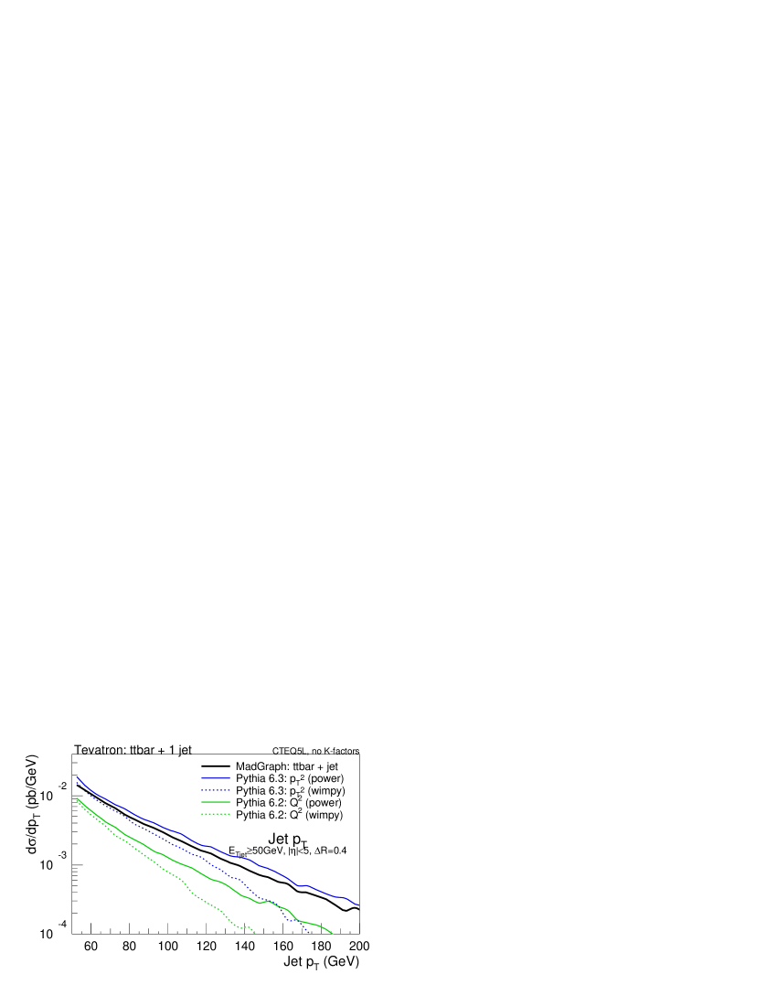
Figure 2: The Tevatron $\mathrm{t}\bar{\mathrm{t}}$+jet rate as a function of jet $p_{\perp}$. Results are shown for MadGraph, and for hard (‘power’) and soft (‘wimpy’) variants of both the $Q^{2}$– and $p_{\perp}^{2}$–ordered PYTHIA showers, see text.

The ’power’ and ’wimpy’ versions of each shower represent a reasonable range of variation of the maximum scale for shower emissions, with the former populating all available phase space, and the latter bounded by the scale of the hard interaction. Though it is still too early to draw more general conclusions, it is encouraging that both the shape and normalisation of the distribution appear to be improved, especially in the ’power shower’ variant of the $p_{\perp}$–ordered algorithm.

4 The Underlying Event

The underlying event may be defined somewhat loosely as the activity in a (single) hadron–hadron collision which does not originate directly from the hard scattering that triggered the event. Currently, this component is not well understood from first principles. What is known, on the other hand, is that it produces omnipresent systematic as well as random fluctuations in activity, which impact isolation criteria, jet energy scales, etc., which can be of significant magnitude for experimental analyses.

During the last few years it has become increasingly clear that the underlying event not only contains soft activity but also has a semi–hard, ’lumpy’ component Field (2002–2003). To explain this, the concept of multiple perturbative interactions Sjöstrand and van Zijl (1987) appears increasingly attractive. Several recent implementations are built on ideas incorporating multiple interactions in one form or another, including the underlying–event framework in the HERWIG add–on JIMMY Butterworth et al. (1996), the new interleaved model Sjöstrand and Skands (2004, 2005) in PYTHIA 6.3, and the underlying–event model being developed for SHERPA Schumann (2004), this latter being quite similar to the old PYTHIA one Sjöstrand and van Zijl (1987).

The most recent development has been the interleaved model of Sjöstrand and Skands (2004, 2005). In this picture, the evolution of the initial state radiation and the generation of multiple scatterings are no longer independent. Instead, a successive ‘fine-graining’ of all the perturbative activity is performed, with radiations interspersed (or ‘interleaved’) with interactions. This allows correlations to be introduced between all the perturbative activity at successively smaller scales. For instance, the third interaction will know about the presence of a gluon having been radiated off a valence quark in the first, etcetera. This introduces for the first time non–trivial correlations in flavour and $x$, while all known sum rules are still respected (e.g. momentum conservation and quark counting rules). In addition, the model allows new possibilities for impact parameter dependence, and contains a more refined treatment of beam remnants, based on an extension of the Lund string model to ‘baryonic’ colour topologies Sjöstrand and Skands (2003).

With the development of more sophisticated physics models, the hope is that it will be possible to ask a range of more meaningful physics questions, among which especially the topic of colour correlations and colour reconnections (in view of a possible difference between the vacua left by ${\mathrm{e}}^{+}$${\mathrm{e}}^{-}$ and hadronic initial states) is presently the most actively investigated. Finally, the energy dependence of the underlying activity is currently very poorly known; further studies aiming to pin down the scaling behaviour, for instance by including the available RHIC $\mathrm{p}$$\mathrm{p}$ data, would be of great interest.

5 Conclusion

The quest for the cause of electroweak symmetry breaking is (hopefully) nearing its end. Should the Tevatron not discover it within a few years, the experimental programme at the LHC promises a comprehensive exploration of the TeV scale, with the emphasis on precisely this question, as well as on more general searches for signals of physics beyond the Standard Model. In addition, the high energies and hadronic environment of both the Tevatron and in particular the LHC will challenge our understanding of QCD, especially our ability to solve it for large numbers of partons, both real and virtual, and our control of phenomena near the borders of its perturbative domain.

It is encouraging, then, to see a truly impressive effort mounted in recent years to address several of the most important issues, among which I have here discussed more precise and realistic simulation of events at higher perturbative orders, improved parton shower models, and some progress towards a better understanding of the underlying event.

On a general note, the emergence of many sophisticated but specialised tools entails an increased need for efficient cross–communication between the programs. For instance, while the traditional Monte Carlo generators have been largely self-contained in the past, the time-consuming process of hard–coding matrix elements for each process by hand can now be left to automatic programs optimised specifically for this task. One should therefore expect an increased reliance on external interfaces, such as provided by the Les Houches Accords Boos et al. (2001); Skands et al. (2004), in the future.

Finally, though much of the effort reported here is still centred around a relatively few groups, for which simple manpower restrictions often represent a non–trivial problem, the many new and exciting developments do seem to have led to an increased communication, bringing people together from different fields. Hopefully, with continued nourishment, this is a trend that will continue and grow in the future.

References

- Pumplin (2005) J. Pumplin, “Parton Distributions,” in these proceedings, 2005, transparencies available from www.hep.wisc.edu/dis05/.
- Stump (2005) D. Stump, “Stability and uncertainty of parton distribution functions,” in these proceedings, 2005, transparencies available from www.hep.wisc.edu/dis05/.
- Thorne (2005) R. Thorne, “MRST PDFs and impact on LHC physics,” in these proceedings, 2005, transparencies available from www.hep.wisc.edu/dis05/.
- Pukhov et al. (1999) A. Pukhov, et al. (1999), hep-ph/9908288.
- Yuasa et al. (2000) F. Yuasa, et al., Prog. Theor. Phys. Suppl., 138, 18–23 (2000), hep-ph/0007053.
- Tsuno et al. (2003) S. Tsuno, et al., Comput. Phys. Commun., 151, 216–240 (2003), hep-ph/0204222.
- Murayama et al. (1991) H. Murayama, I. Watanabe, and K. Hagiwara (1991), kEK-91-11.
- Stelzer and Long (1994) T. Stelzer, and W. F. Long, Comput. Phys. Commun., 81, 357–371 (1994), hep-ph/9401258.
- Maltoni and Stelzer (2003) F. Maltoni, and T. Stelzer, JHEP, 02, 027 (2003), hep-ph/0208156.
- Moretti et al. (2001) M. Moretti, T. Ohl, and J. Reuter (2001), hep-ph/0102195.
- Krauss et al. (2002) F. Krauss, R. Kuhn, and G. Soff, JHEP, 02, 044 (2002), %****␣dis_05_proc2.bbl␣Line␣50␣****hep-ph/0109036.
- Kawabata (1995) S. Kawabata, Comp. Phys. Commun., 88, 309–326 (1995).
- Ilyin et al. (1996) V. A. Ilyin, D. N. Kovalenko, and A. E. Pukhov, Int. J. Mod. Phys., C7, 761 (1996), hep-ph/9612479.
- Mangano et al. (2003) M. L. Mangano, M. Moretti, F. Piccinini, R. Pittau, and A. D. Polosa, JHEP, 07, 001 (2003), hep-ph/0206293.
- Campbell and Ellis (2000) J. M. Campbell, and R. K. Ellis, Phys. Rev., D62, 114012 (2000), hep-ph/0006304.
- Beenakker et al. (1996) W. Beenakker, R. Hopker, and M. Spira (1996), hep-ph/9611232.
- Berends et al. (1989) F. A. Berends, W. T. Giele, and H. Kuijf, Phys. Lett., B232, 266 (1989).
- Berends et al. (1991) F. A. Berends, H. Kuijf, B. Tausk, and W. T. Giele, Nucl. Phys., B357, 32–64 (1991).
- Giele et al. (1993) W. T. Giele, E. W. N. Glover, and D. A. Kosower, Nucl. Phys., B403, 633–670 (1993), hep-ph/9302225.
- Kersevan and Richter-Was (2003) B. P. Kersevan, and E. Richter-Was, Comput. Phys. Commun., 149, 142–194 (2003), hep-ph/0201302.
- Nagy and Trocsanyi (1999) Z. Nagy, and Z. Trocsanyi, Phys. Rev., D59, 014020 (1999), hep-ph/9806317.
- Banfi et al. (2005) A. Banfi, G. P. Salam, and G. Zanderighi, JHEP, 03, 073 (2005), hep-ph/0407286.
- Amati et al. (1980) D. Amati, A. Bassetto, M. Ciafaloni, G. Marchesini, and G. Veneziano, Nucl. Phys., B173, 429 (1980).
- Webber (1986) B. R. Webber, Ann. Rev. Nucl. Part. Sci., 36, 253 (1986).
- Gustafson and Pettersson (1988) G. Gustafson, and U. Pettersson, Nucl. Phys., B306, 746 (1988).
- Lönnblad (1992) L. Lönnblad, Comput. Phys. Commun., 71, 15–31 (1992).
- Lönnblad (1996) L. Lönnblad, Nucl. Phys., B458, 215–230 (1996), hep-ph/9508261.
- Marchesini and Webber (1984) G. Marchesini, and B. R. Webber, Nucl. Phys., B238, 1 (1984).
- Seymour (1995) M. H. Seymour, Comp. Phys. Commun., 90, 95–101 (1995), hep-ph/9410414.
- Corcella et al. (2001) G. Corcella, et al., JHEP, 01, 010 (2001), hep-ph/0011363.
- Gieseke et al. (2003) S. Gieseke, P. Stephens, and B. Webber, JHEP, 12, 045 (2003), hep-ph/0310083.
- Bengtsson and Sjöstrand (1987) M. Bengtsson, and T. Sjöstrand, Nucl. Phys., B289, 810 (1987).
- Norrbin and Sjöstrand (2001) E. Norrbin, and T. Sjöstrand, Nucl. Phys., B603, 297–342 (2001), hep-ph/0010012.
- Sjöstrand et al. (2001) T. Sjöstrand, et al., Comput. Phys. Commun., 135, 238–259 (2001), hep-ph/0010017.
- Sjöstrand and Skands (2005) T. Sjöstrand, and P. Z. Skands, Eur. Phys. J., C39, 129–154 (2005), hep-ph/0408302.
- Gleisberg et al. (2004) T. Gleisberg, et al., JHEP, 02, 056 (2004), hep-ph/0311263.
- Sjöstrand and Skands (2003) T. Sjöstrand, and P. Z. Skands, Nucl. Phys., B659, 243 (2003), hep-ph/0212264.
- Corcella and Moretti (2004) G. Corcella, and S. Moretti (2004), hep-ph/0402149.
- Miu and Sjöstrand (1999) G. Miu, and T. Sjöstrand, Phys. Lett., B449, 313–320 (1999), hep-ph/9812455.
- Andre and Sjöstrand (1998) J. Andre, and T. Sjöstrand, Phys. Rev., D57, 5767–5772 (1998), hep-ph/9708390.
- Mrenna (1999) S. Mrenna (1999), hep-ph/9902471.
- Mangano (2004) M. Mangano, ”The so–called MLM prescription for ME/PS matching” (2004), Talk presented at the Fermilab ME/MC Tuning Workshop, October 4, 2004.
- Catani et al. (2001) S. Catani, F. Krauss, R. Kuhn, and B. R. Webber, JHEP, 11, 063 (2001), hep-ph/0109231.
- Krauss (2002) F. Krauss, JHEP, 08, 015 (2002), hep-ph/0205283.
- Lönnblad (2002) L. Lönnblad, JHEP, 05, 046 (2002), hep-ph/0112284.
- Mrenna and Richardson (2004) S. Mrenna, and P. Richardson, JHEP, 05, 040 (2004), hep-ph/0312274.
- Frixione (2005) S. Frixione, “Monte-Carlo generators,” in these proceedings, 2005, transparencies available from www.hep.wisc.edu/dis05/.
- Lavesson and Lönnblad (2005) N. Lavesson, and L. Lönnblad (2005), hep-ph/0503293.
-
Mrenna (2004)
S. Mrenna, Patriot database (2004), see
http://cepa.fnal.gov/personal/mrenna/Matched_Dataset_Description.html. - Dobbs (2002) M. Dobbs, Phys. Rev., D65, 094011 (2002), hep-ph/0111234.
- Potter and Schorner (2001) B. Potter, and T. Schorner, Phys. Lett., B517, 86–92 (2001), %****␣dis_05_proc2.bbl␣Line␣200␣****hep-ph/0104261.
- Collins (2000) J. C. Collins, JHEP, 05, 004 (2000), hep-ph/0001040.
- Collins and Hautmann (2001) J. C. Collins, and F. Hautmann, JHEP, 03, 016 (2001), hep-ph/0009286.
- Collins and Zu (2005) J. C. Collins, and X. Zu, JHEP, 03, 059 (2005), hep-ph/0411332.
- Frixione and Webber (2002) S. Frixione, and B. R. Webber, JHEP, 06, 029 (2002), hep-ph/0204244.
- Frixione et al. (2003) S. Frixione, P. Nason, and B. R. Webber, JHEP, 08, 007 (2003), hep-ph/0305252.
- Kramer and Soper (2004) M. Kramer, and D. E. Soper, Phys. Rev., D69, 054019 (2004), hep-ph/0306222.
- Soper (2004) D. E. Soper, Phys. Rev., D69, 054020 (2004), hep-ph/0306268.
- Nagy and Soper (2005) Z. Nagy, and D. E. Soper (2005), hep-ph/0503053.
- Gieseke et al. (2004) S. Gieseke, A. Ribon, M. H. Seymour, P. Stephens, and B. Webber, JHEP, 02, 005 (2004), hep-ph/0311208.
- Sjöstrand et al. (2003) T. Sjöstrand, L. Lönnblad, S. Mrenna, and P. Skands (2003), hep-ph/0308153.
- Krauss et al. (2005) F. Krauss, A. Schalicke, and G. Soff (2005), hep-ph/0503087.
- Webber (1984) B. R. Webber, Nucl. Phys., B238, 492 (1984).
- Gieseke (2004) S. Gieseke (2004), hep-ph/0408034.
- Gieseke (2005) S. Gieseke, JHEP, 01, 058 (2005), hep-ph/0412342.
- Gustafson (1986) G. Gustafson, Phys. Lett., B175, 453 (1986).
- Rudolph (2003) G. Rudolph (2003), ALEPH, unpublished.
- Huston et al. (2004) J. Huston, I. Puljak, T. Sjöstrand, and E. Thomé, “Resummation and shower studies,” in The QCD/SM working group: Summary report, 3rd Les Houches Workshop: Physics at TeV Colliders, Les Houches, France, 26 May - 6 Jun 2003, M. Dobbs et al., hep-ph/0403100, 2004, hep-ph/0401145.
- Plehn et al. (2005) T. Plehn, D. Rainwater, and P. Skands (2005), in preparation.
- Field (2002–2003) R. Field, presentations at the ‘Matrix Element and Monte Carlo Tuning Workshop, Fermilab, 4 October 2002 and 29–30 April 2003 (2002–2003), talks available from webpage http://cepa.fnal.gov/CPD/MCTuning/, and further recent talks available from http://www.phys.ufl.edu/rfield/cdf/.
- Sjöstrand and van Zijl (1987) T. Sjöstrand, and M. van Zijl, Phys. Rev., D36, 2019 (1987).
- Butterworth et al. (1996) J. M. Butterworth, J. R. Forshaw, and M. H. Seymour, Z. Phys., C72, 637–646 (1996), hep-ph/9601371.
- Sjöstrand and Skands (2004) T. Sjöstrand, and P. Z. Skands, JHEP, 03, 053 (2004), hep-ph/0402078.
- Schumann (2004) S. Schumann, SHERPA: an event generator for the LHC (2004), talk given at HERA/LHC Workshop, CERN, October 2004.
- Boos et al. (2001) E. Boos, et al. (2001), hep-ph/0109068.
- Skands et al. (2004) P. Skands, et al., JHEP, 07, 036 (2004), hep-ph/0311123.